Message passing theory for percolation models
on multiplex networks with link overlap
Abstract
Multiplex networks describe a large variety of complex systems including infrastructures, transportation networks and biological systems. Most of these networks feature a significant link overlap. It is therefore of particular importance to characterize the mutually connected giant component in these networks. Here we provide a message passing theory for characterizing the percolation transition in multiplex networks with link overlap and an arbitrary number of layers . Specifically we propose and compare two message passing algorithms, that generalize the algorithm widely used to study the percolation transition in multiplex networks without link overlap. The first algorithm describes a directed percolation transition and admits an epidemic spreading interpretation. The second algorithm describes the emergence of the mutually connected giant component, that is the percolation transition, but does not preserve the epidemic spreading interpretation. We obtain the phase diagrams for the percolation and directed percolation transition in simple representative cases. We demonstrate that for the same multiplex network structure, in which the directed percolation transition has non-trivial tricritical points, the percolation transition has a discontinuous phase transition, with the exception of the trivial case in which all the layers completely overlap.
pacs
89.75.Fb, 64.60.aq, 05.70.Fh, 64.60.ahI Introduction
Multilayer networks [1, 2, 3] describe complex systems formed by different interacting networks. Examples of multilayer networks are ubiquitous, ranging from infrastructures and transportation networks to cellular and brain networks [4, 5, 6, 7, 8, 9, 10]. Characterizing the robustness of multilayer networks is important for predicting the response to damage of infrastructures, transportation networks and biological networks. In multilayer networks, nodes from different layers are often interdependent. The interdependence between nodes implies that a node is damaged if its interdependent nodes are damaged. Recently a generalized percolation process has been proposed to study the robustness of multilayer networks in the presence of interdependencies [11, 12, 13]. This model allows to understand and to control the fragility of interconnected infrastructures. It also enables us to describe possible scenarios for generalized percolation processes.
Percolation on single random (locally tree-like) networks can be treated with tools exploiting the locally tree-like approximation [14] familiar to statistical mechanics and, alternatively, with message passing algorithms [15, 16, 17]. Notably, the challenge of going beyond the tree-like approximations has been addressed in complex networks either by considering percolation on self-similar networks [18] or, more recently, by modifying and generalizing message passing algorithms [19].
In single networks, the percolation transition, leading to the emergence of the giant connected component in a network, is a continuous phase transition. A generalization of the giant connected component for multilayer networks with interdependencies between the nodes is called a mutually connected giant component (MCGC) [11, 12, 13]. As the fraction of damaged nodes increases, a discontinuous, hybrid phase transition occurs, after which the MCGS emerges, and the response of the system to perturbation is characterized by large avalanches of failure events that propagate back and forth between different layers [11]. Interestingly, the hybrid phase transition combines a discontinuity and a critical singularity. The nature of this phase transition is a clear sign that multilayer networks with interdependencies display a significant fragility with respect to random damage. Several other generalized percolation problems on multiplex networks have been also proposed, including competition between the layers [20, 21], weak percolation [22, 23], generalized -core percolation [24], percolation on directed multiplex networks [25], spanning connectivity [26], and bond percolation [27].
The emergence of the MCGC has been studied on a variety of multilayer structures including multiplex networks [11, 12, 13, 29, 30, 31, 32, 33] and networks of networks [34, 35, 36]. Networks of networks are multilayer networks formed by different networks (layers), where the nodes of different networks might be related by interdependencies. The percolation transition in these networks is significantly affected by the way the links implying interdependencies are placed, and, moreover, instead of single, there may be multiple transitions [35, 36].
Multiplex networks describe a large variety of complex systems and constitute a well controlled setting to study the interplay between structure and dynamics in multilayer networks. They are formed by a set of nodes interacting via different layers. Each node has a replica node in each layer, and each layer is a distinct network for the replica nodes in that layer. The interdependencies in multiplex networks are usually placed between the replica nodes from different layers. The percolation phase transition describing the emergence of the MCGC in multilayer networks, with layers formed by random networks with given degree distributions, has been fully characterized as a discontinuous and hybrid transition [11, 12]. The phase transition remains hybrid and discontinuous in the presence of correlations in the degrees of replica nodes [29] but can become a continuous in the case of partial interdependence [30, 31, 32] or if some nodes are not active (not connected) in each layer [33, 10]. Interestingly, these results can be obtained using a locally tree-like approximation, or equivalently, a message passing algorithm which admits an epidemic spreading interpretation [13, 28].
Numerous multilayer networks have a significant link overlap [37, 4, 7, 9], which explains the need to explore the percolation transition on this type of correlated multilayer structures [38]. Recently, two approaches were used to describe the transition in duplex networks (i.e. networks formed by layers) with link overlap. The first approach consists of a coarse-grained description of the multiplex network in terms of supernodes [39, 40]. The second approach is instead based only on a traditional local tree-like approximation [41]. Interestingly, it turns out that a message passing algorithm that admits an epidemic spreading interpretation [42, 43], inspired by the algorithm originally proposed for multiplex network without link overlap, does not capture the MCGC [39, 40, 41], but instead characterizes a new type of directed percolation. This process can be interpreted as a variation of a bootstrap percolation dynamics [44, 22] or a as the viability percolation problem [40] in the limit in which the resource nodes are vanishing. Here we call this dynamical process directed percolation and its order parameter directed mutually connected giant component (DMCGC) to distinguish it from the MCGC. The choice of this terminology is due to the fact that we want to highlight the directed nature of the underlying process, and the connection to epidemic spreading [45] processes nevertheless we want to clarify that the links of the underlying multiplex network do not have an intrinsic directionality.
Our unified approach to percolation and directed percolation is directly applicable to multiplex network with link overlap and arbitrary number of layers . This approach is used to fully characterize and compare the percolation transitions and the directed percolation transitions on ensembles of random multiplex networks. We show that while the directed percolation transition in multiplex networks with link overlap can have non-trivial tricritical points, the percolation transition on this type of multiplex networks is always hybrid and discontinuous with the sole trivial exception in that all the layers of a multiplex network completely overlap with each other.
Message passing algorithms are attracting increasing attention in network theory. They were used to characterize the structure of single networks [43] or epidemic spreading in temporal multi-slices networks [46], and to detect the driver nodes controlling a network [47]. This work shows that a new class of message passing algorithms can be used to investigate the structure of multiplex networks with link overlap, allowing to characterize both the MCGC and DMCGC in locally tree-like networks.
Interestingly, the DMCGC is related to directed cooperative epidemic spreading in multiplex networks, while the MCGC characterizes the response of the interdependent multiplex network structure to external damage.
The DMCGC model could provide therefore an ideal setting to extend models of cooperative contagion studied on single networks [48] to multilayer networks.
In Sec. II and III we recall the configuration model for multiplex networks and the definition of mutually connected giant component (MCGC). In Sec. IV we report the message passing theory for calculating the MCGC in multiplex networks without link overlap, using the formalism of Ref. [37]. In Sec. V we present the multilink definitions in the case of link overlap, using the formalism of Ref. [42]. In Sec. VI, we clarify the extension of the message passing approach to multiplex networks with link overlap. We distinguish between two possible extensions, leading to a directed mutually connected giant component (DMCGC) and a mutually connected giant component (MCGC), respectively. In Sec. VII we briefly describe the results obtained with DMCGC. The main novel contribution of this paper is in Sec. VIII, where we define the message passing approach for MCGC in the presence of link overlap, and present results for a few particular cases. Finally, Sec. IX reports our conclusions.
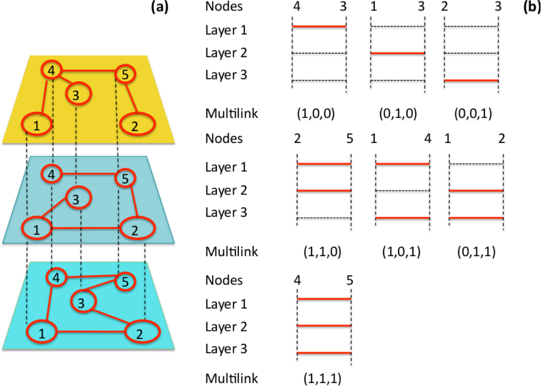
II Multiplex networks without link overlap
A multiplex network is formed by a set of nodes interacting through layers with each layer formed by a distinct network . Every node has replica nodes, one for each layer indicating the node identity in layer . Replica nodes are connected pairwise by interlinks. Figure 1 shows an example of a multiplex network with layers. A network in layer connects the replica nodes in this layer. This network is fully described by the adjacency matrix . The matrix element of the adjacency matrix indicates whether node is connected to node in layer () or not ().
In a multiplex network, we define the total overlap [37] of the links in layer and layer as the total number of pairs of nodes connected both in layer and layer , i.e.
| (1) |
Additionally we define [37] for each node the local overlap of the links in layer and layer as the total number of neighbors of node which are simultaneously neighbors in layer and in layer , i.e.
| (2) |
We stress that most real multiplex networks have a significant total and local overlap of their links [4, 7, 9].
The first natural approach to construct an ensemble of random multiplex networks, is to generate each layer independently. For this, we draw the sequence of the degrees of each node from a given degree distribution . If the degrees of each individual node in different layers are uncorrelated, the degree distribution factorizes as
| (3) |
where is the degree distribution in layer . Finally, having assigned to each node the degree in every layer , we can construct a multiplex network in which each layer is a random graph with given degree sequence , i.e. we consider a random multiplex chosen with probability
| (4) |
where here and in the following indicates the Kronecker delta. As long as the layers are formed by sparse networks, and the number of layers is much smaller than the number of nodes, i.e. , the multiplex network constructed in this way has a negligible total link overlap between any two layers and , and a negligible local overlap also [37]. Since the link overlap is a general property of multiplex networks, one should consider multiplex network models able to reproduce this structural feature. Such models have been introduced in [37] and will be discussed in Sec. V.
For the sake of simplicity we will assume throughout the paper that each node is active (i.e. connected) in every layer. This assumption can be relaxed. We refer the interested reader to Refs. [10, 33, 26] where this case and its implications for the percolation transition, including asymptotic behavior in case of a large number of layers, are discussed in detail.
III Percolation on multiplex networks and mutually connected giant component
In this paper we consider the robustness of multiplex networks in the presence of interdependencies.
Following Ref. [11] we assume that each interlink indicates an interdependency between the linked replica nodes. This interdependencies imply that if a replica node is damaged, then all the interdependent replica nodes in the other layers are damaged. The robustness of the multiplex network is monitored by the response to an external initial damage performed on a set of nodes of the network. The variables , where , fully characterize the inital damage to the network, as each variable indicates whether node has been initially damaged () or not (). The multiplex network responds non-linearly to this damage as it can be quantifying by the size of its mutually connected giant component (MCGC). The MCGC has been defined in [11] as a generalization of the giant component of single networks. This is the component that remains after the damage propagates back and forth between the layers. The original algorithm that defines the MCGC is the following:
- (i)
the giant component of each layer is determined, evaluating the effect of the damaged nodes in each single layer;
- (ii)
each node that has at least a replica node not in the giant component of its proper layer is damaged, i.e. all its replica nodes are damaged due to the interdependencies existing between them;
- (iii)
If there are no new damaged nodes the algorithm stops, otherwise it proceed, starting again from step (i).
At the end of the iteration the nodes that are not damaged by the iterative process form the MCGC. The size of the MCGC is given by the number of nodes remaining undamaged by this process. If the initial damage has probability distribution
| (5) |
i.e. initially each node is damaged independently with probability , we observe a phase transition with the order parameter and the control parameter .
IV Percolation in multiplex networks without link overlap
IV.1 The message passing algorithm
On a locally tree-like multiplex network without link overlap, the MCGC can be found by using a suitable message passing algorithm. This algorithm has been first proposed by Son et al. [13]. According to this algorithm, nodes send messages along their links to neighbor nodes. Each message sent by a node to a node indicates whether node belongs to the MCGC also in absence of the link . In particular the message that node send to a neighbor node in layer is equal to one () if the following conditions are met:
- (a)
node is not initially damaged, i.e. ;
- (b)
node belongs to the mutually connected giant component even if the link between node and node is removed from the multiplex, i.e. for every layer node receives at least one positive message from nodes that are neighbors of node in layer .
If these conditions are not met, then . These messages determine whether a node belongs () or not () to the MCGC. In fact node belongs to the MCGC () if and only if
- (a)
node is not initially damaged;
- (b)
node receives at least one positive message from a neighbor of node in every layer .
These two algorithms directly translate in the message passing equations
| (6) |
where indicates the set of neighbors of node in layer . Let us consider a random multiplex network taken with probability given by Eq. (4) and a random realization of the initial damage described by the probability given by Eq. (5). The average message in layer , and the (relative) average number of nodes in the MCGC, are given by
| (7) | |||||
If there are no correlations between the degrees of a node in different layers, and so the degree distribution follows Eq. (3), then we have
| (8) |
Here the generating functions and of the degree distribution of layer are given by
| (9) |
IV.2 The case of equally distributed Poisson layers
In the case of equally distributed Poisson layers with average degree , we have
| (10) |
for every layer . Then, using Eqs. (8), one can show that for every layer , and is determined by the equation
| (11) |
By setting , this equation reduces to , where the function is
| (12) |
This equation has always the trivial solution . In addition, a non-trivial solution indicating the presence of the MCGC, emerges at a hybrid discontinuous transition at , determined by the equations
| (13) |
For this yields the discontinuous hybrid transition for , [11, 13, 12]. For this yields the discontinuous hybrid transition for , .
V Multiplex networks with link overlap
The vast majority of multiplex networks in infrastructures, transport, social and collaboration networks are characterized by significant link overlap [4, 7, 9]. Therefore it is of crucial importance to determine the robustness of multiplex networks in presence of this structural feature. In order to model multiplex networks with link overlap, the notion of multilinks [37, 9, 42] turns out to be extremely useful. Two nodes and are connected by a multilink with , if and only if they are linked in every layer for which and they are not linked in every layer for which (see Fig. 1 for a graphical description of multilinks). We distinguish between the non-trivial multilinks and the trivial multilink indicating the absence of any sort of link between the two nodes.
Using the concept of multilinks one can define multi-adjacency matrices whose element indicates whether node is connected to node by a multilink () or not . The multi-adjacency matrices encode the same information encoded in the adjacency matrices and the matrix elements can consequently be expressed as a function of the matrix elements as
| (14) |
The multi-adjacency matrices are not independent in in the sense that they satisfy
| (15) |
for every pair of nodes of the multiplex network. Having introduced the multi-adjacency matrices it is straightforward to define the multidegrees [37, 9, 42]. The multidegree of node indicated as is the sum of rows (or column) of the multi adjacency matrix , i.e.
| (16) |
Therefore, the multidegree indicates the number of nodes linked to node by a multilink . As an example, consider a multiplex network (duplex) formed by two layers. Using the adjacency matrices of elements , the multidegrees of node are given by
| (17) |
From the explicit expression of the multidegree it is evident that this quantity is given by the local overlap defined in Eq. (2), i.e.
| (18) |
Therefore indicates the number of neighbors of node that are simultaneously neighbor in layer and layer . On the contrary, the multidegree / indicate respectively the number of neighbors of node that are neighbor in layer 1/(layer 2) but not in layer 2/(layer 1). Finally the multidegree indicates the total number of nodes that are not connected to node in any layer.
In general, for arbitrary (but finite) number of layer , the multidegrees of a node give a complete, local information about the link overlap in different layers.
Naturally, since the multiadjacency matrices are not independent, also the multidegrees of a node are not all independent, and we have
| (19) |
for every node , which can also be written as
| (20) |
In a sparse multiplex network the non-trivial multidegrees with have finite average .
Random multiplex networks with a given distribution of the multidegree sequence provide the easiest way to generate multiplex networks with a controlled link overlap. In order to do this we first draw the sequence of multidegrees of each node from the multidegree distribution . To each node we associate stubs of type and finally we match pairwise stubs of the same multilink type. In this way the probability that node and node are connected by a multilink is given by [37]
| (21) |
as long as the multidegrees have the natural structural cutoff, i.e.
| (22) |
for every multilink . In this ensemble the probability of a multiplex is given by
| (23) |
Eventually, the multidegrees of a given node can be uncorrelated, i.e. the multidegree distribution factorizes
| (24) |
where is the distribution of multidegrees with .
VI Mutually connected component and Directed mutually connected component in multiplex networks with link overlap
The message passing algorithm discussed in Sec. IV can be extended and used to explore the structure of locally tree-like multiplex networks with link overlap in different ways. We consider two extensions. With the first algorithm (Sec. VII), one characterizes the directed mutually connected giant component (DMCGC), with the second algorithm (Sec. VIII) one characterizes the mutually connected giant component (MCGC). Both algorithms reduce to the algorithm studied in Sec. IV in the absence of link overlap. Moreover, both algorithms reduce to percolation on a single network in the presence of complete overlap of all the layers. The algorithm [42] that calculates the DMCGC has an epidemic spreading interpretation and an inherent directed character. In this epidemic spreading interpretation, we assume that a different disease propagate in each layer of the multiplex networks and that a node is infected (i.e. it sends a positive message to a downstream node) only if it is in contact to at least an infected upstream neighbor in every layer . The set of nodes that become infected are the nodes in the DMCGC. It has been shown that this algorithm determines a proper subset of the nodes that are in the MCGC as soon as there is link overlap [40]. For example, for the network in Fig. 2, all the nodes of the drawn networks belong to the MCGC, but, according to the message passing algorithm with the epidemic spreading interpretation, two nodes remain uninfected. That is, while these two nodes belong to the MCGC, they do not belong to the DMCGC [40].
It has been debated if a message passing algorithm allows to describe the mutually connected giant component in multiplex networks with an arbitrary number of layers . Recently a traditional tree-like approximation was successfully used to characterize the mutually connected giant component in a multiplex networks with link overlap and [41]. Here we show that it is possible to extend these results to multiplex network with arbitrary number of layers and link overlap by using a message passing algorithm combined with the use of multilinks.
In the following we treat and compare two different types of message passing algorithms: one for directed percolation and the other for percolation, which can detect the nodes belonging respectively to the DMCGC and to the MCGC. Applying these algorithms one can study the critical properties of the two percolation transitions and observe significant changes in the phase diagrams of these problems. In Sec. VII, we describe directed percolation and then, in Sec. VIII, we calculate the size of the MCGC with the message passing approach, in multiplex networks with link overlap.

VII Directed percolation of multiplex networks
VII.1 The message passing algorithm
In a locally tree-like multiplex with link overlap a simple extension of the message passing from Sec. IV determines the set of nodes belonging to the directed mutually connected giant component (DMCGC) [42]. Let indicate if a node is removed or not from the network and let be the indicator function that the node is in the DMCGC. The value of is determined by the “messages” that the neighboring nodes send to node . We denote the message sent from node to node as . The value of this is set to one if and only if the following three conditions are satisfied:
- (a)
node is a neighbor of node with a multilink connecting them such that ;
- (b)
node is not initially damaged, i.e. ;
- (c)
node belongs to the directed mutually connected giant component even if the multilink between node and node is removed from the multiplex, i.e. node receives at least one positive message from a nearest neighbor in every layer .
If any of these conditions is not satisfied then the messages is zero, i.e. .
Additionally, node is in the DMCGC () if the following conditions are satisfied:
- (a)
node is not initially damaged
- (b)
for every layer node receives at least one positive message from a neighbors in layer .
This algorithm directly translates into the following message passing equations for and :
| (25) | |||
| (26) |
where indicates the set of neighboring nodes of node in layer . Let us consider a random realization of the initial damage drawn from the probability distribution given by Eq. (5) and a random realization of the multiplex network with link overlap chosen with probability given by Eq. (23). The average message along a generic multilink and the average number of nodes in the DMCGC are respectively given by (see Ref. [42] for the details of the derivation)
| (27) | |||||
where with and if and otherwise (see Ref. [42] for the details of the derivation). For uncorrelated multidegrees of the nodes, when the distribution follows Eq. (24), these equations read
| (28) | |||||
where and have the same definition as above, and the generating function and are given by
| (29) |
Note that this algorithm and therefore Eqs. (28) reduce to the Eqs. (9) found in Sec. IV in the absence of link overlap, i.e. where the only non-trivial multilinks are the ones with .
Here we show two simple examples of how this scheme works in practice. These examples have been already discussed in [42] and checked against simulation results in [40] but we report them here to demonstrate the difference between the equation determining the DMCGC and the one for the MCGC that we calculate for the same multiplex ensembles in Sec. VIII.3 and Sec. VIII.4.
VII.2 Two Poisson layers with Overlap
We consider now the case of a duplex in which the multidegree distributions are Poisson with , and . Due to the properties of the Poisson distribution, we have , for every , where satisfies the equation
| (30) |
By setting , and we can study the solutions of the equivalent equation
| (31) |
in the parameter plane. The critical line of discontinuous hybrid transition is found by solving the system of equations
| (32) |
The critical line of second order phase transition is found by solving the equation
| (33) |
We notice that there is a non-trivial critical point for for which
| (34) |
The full phase diagram of the model is displayed in Fig. 3. We note that for the transition is hybrid and discontinuous and reduces to the know transition in duplex network with no link overlap, while for of complete overlap of the layers the transition is continuous and reduces to the percolation transition on a single Poisson network.
VII.3 Three Poisson Layers with Overlap
As a second example, we consider the ensemble of a three layer multiplex network with a Poisson multi-degree distribution and , and . As in the previous case, we have one order parameter , and satisfies the equation
| (35) | |||||
By setting , and we can define a function as
| (36) | |||||
and we can recast the equation for as .
The phase diagram of this directed percolation problem is very rich. It includes non-trivial tricritical points. We refer the interested reader to the paper [42] that investigate this case in detail. Additionally we observe here that for we recover the prediction of the percolation transition in interdependent multiplex network with no link overlap, while for we recover the results of the percolation transition on a single Poisson network.
VIII Percolation with link overlap
VIII.1 General observations on the message passing algorithm for the MCGC
Message passing algorithms are powerful methods, allowing to solve exactly graphical models on locally tree-like networks, i.e. networks with a vanishing density of finite cycles. These methods are versatile, as they can be applied not only to ensembles of random networks, but also to single network realizations. For these reasons these algorithms are becoming increasingly popular in network science with applications ranging from percolation on single and multilayer networks to controllability [15, 28, 13, 35, 36, 43, 47]. These algorithms proceed by iteration of dynamical rules which determine messages or beliefs that a node sent to a neighboring node. In general, these beliefs indicate the probability that the neighbor node is in a given dynamical state and take real variables between zero and one. Percolation on single networks, as well as generalized percolation problems defined for multiplex networks, are inherently optimization problems in which one aims at characterizing the giant component, which is the largest connected component satisfying a set of conditions. In this case the messages polarize and take only value , as we have already seen in the cases discussed so far.
Moreover, in general, messages sent from node to a downstream node take into account not only the states of the upstream nodes but also the state of node . We show that the message passing algorithm that determines the nodes in the MCGC of a multiplex network with overlap has the following properties: it is polarized (i.e. the messages take values ) and assumes that the downstream node belongs to the MCGC. These two properties of the message passing algorithm are in agreement with the general definition of the message passing algorithm, nevertheless, due to the second property, the resulting algorithm for detecting the MCGC loses the epidemic spreading interpretation when compared to the algorithm used to detect the DMCGC.
VIII.2 The message passing algorithm
Let indicate if a node is removed or not from the network and let be the indicator function that the node is in the mutually connected giant component. Let also be a fixed vector with . The rationale of introducing vector can be explained with the help of Fig. 4 that highlights the difference between DMCGC and MCGC [49]. In order to evaluate if node is in the MCGC, it is not sufficient to assume only the information upstream from node . In fact, we must encode a system of messages that may reach node through different paths, on different layers. In the network of Fig. 4, node belongs to the MCGC because it is reached by a positive message on layer 1 (solid) through node and by a positive message on layer 2 (dashed) through node . Therefore, our aim is to define the minimal set of layers that allows node to connect node to the MCGC through node . For a given multilink , we will define below a vector that encodes this selected set of layers.
Let us formally define our message passing algorithm that determines if a node is in the MCGC in a locally tree-like multiplex network. The value of is determined by the “messages” that the neighboring nodes send to node . We denote the generic “message” as . These messages are defined for every possible value of , and only for we will have the message indicating that node connects node to the MCGC exclusively through the links where .
Let us now treat separately the cases and . For the value of the message is set to one, , if and only if the following three conditions are satisfied:
- (i)
node is a neighbor of node with a multilink connecting them such that ;
- (ii)
assuming node belongs to the mutually connected giant component, node is in the mutually connected component, i.e. it is not initially damaged and it has at least one neighbor in any layer that belongs to the MCGC;
- (iii)
node connects node to the mutually connected component exclusively through the layers with . This implies that, if , then this condition can only be satisfied if , because otherwise we would need a link to allow for node to be connected to the MCGC on layer through node .
If these three conditions are not met, and , we will have .
An important consequence of this definition is the following. As per condition (iii), having a non-zero message with requires that node connects node to the (unique) MCGC exclusively through the layers with . Then, there can be at most a single vector such that . This vector, if it exists, will encode all the information about all the messages with and will indicate the set of layers that connect node to the MCGC through node . In order to treat at the same level the case in which node connects node to the MCGC at least in one layer and the case in which node does not connect node to the MCGC in any layer, it is convenient to define the messages as it follows:
| (37) |
where is the Kronecker function. Using this definition, we can define the unique vector for which
| (38) |
as
| (39) |
Therefore, the vector is uniquely defined for every linked (ordered) pair of nodes and its components indicate whether node is connected to the MCGC through node in layer () or not ().
Let us now derive the algorithm defining the messages. We first consider condition (ii). Node is in the MCGC if and only if it is not initially damaged and it has at least one nearest neighbor in each layer that it is connected to the MCGC. Assuming that node is in the MCGC, this implies that node should have in each layer for which , at least a neighbor different from node that belongs to the MCGC. Secondly, we consider condition (iii). According to this condition node connects node to the MCGC exclusively through layers for which . Therefore node should have at least a neighbor different from node that belongs to the MCGC in each layer for which , and should not have any neighbor different from node belonging to the MCGC in the layers for which . Therefore the message with is equal to one, , if and only if
- (a)
node is a neighbor of node with a multilink connecting them such that ;
- (b)
node is not initially damaged;
- (c)
for every layer for which either or there is at least one node , neighbor of node in layer , for which ;
- (d)
for every layer for which and every node , neighbor of node in layer , is sending a message with .
An example of this algorithm is schematically sketched in Fig. 5.
Therefore the message passing equation for the messages reads
| (40) | |||||
The value of the indicator function determining if node belongs () or not () to the MCGC depends on the messages . Specifically, node belongs to the MCGC if the following conditions are met:
- (a)
node is not initially damaged, i.e. ;
- (b)
node has at least one neighbor in each layer that connects node to the MCGC, i.e. for which .
Therefore we arrive at the message passing equations determining :
| (41) |
The message algorithm described above, consisting in iterating the Eqs. (40),(39), (37) and (41) allows to predict which nodes of a real locally tree-like multiplex network with link overlap are in the MCGC. The message passing techniques are indeed guaranteed to converge to the correct solution only in locally tree-like networks, although empirically they may work surprisingly well on networks with some small cycles, as long as they have a vanishingly small clustering coefficient in the limit . Considering distributed algorithms that go beyond the tree-like approximation is a long standing challenge that has been tackled by the recent literature [19]. Therefore, it can not be excluded that opportune variations of the algorithm that we have introduced here for locally tree-like networks could be applied in the future to multiplex networks with finite clustering coefficient.
In order to derive the equations for the average messages in ensemble of multiplex networks chosen with probability given by Eq. (23) with random initial damage of the nodes following Eq. (5), let us now consider Eq. (40), by using the formula
| (42) |
valid as long as . Here with , and where the sum is over all possible vectors with in the layers where . Since for each node neighboring node in layer we should necessarily have , we can write
| (43) | |||||
Since and , we can write the above expression as
| (44) | |||||
Finally this expression can be written as
| (45) | |||||
Averaging over the ensemble of multiplex networks where each multiplex network is chosen with probability given by Eq. (23) and the random initial damage with probability given by Eq. (5), we get
| (46) | |||||
with . For networks with an uncorrelated multidegree distribution given by Eq. (24) we get
| (47) | |||||
with .
Similarly in order to derive the equation for let us now transform Eq. (41) by using the formula
where with , and where the sum is over all possible vectors . We expand the multiplications and write
| (48) |
Since and , we can write the above expression as
| (49) |
We average this expression over the ensemble of network by choosing a multiplex network with probability given by Eq. (23) and averaging over the random realization of the initial damage according to the probability distribution in Eq. (5). In this way we get the expression for the average number of nodes in the MCGC:
| (50) | |||||
where is the probability that a node is connected through a multilink to the mutually connected giant component through the layers indicated by the vector . In particular, in an ensemble in which the multi-degree distribution factorizes, i.e. the multidegree distribution follows Eq. (24), we have
| (51) | |||||
Notice that the Eq. (47) and Eq. in the case of networks without link overlap, i.e. where all multilinks have , reduce to the equations found in Sec. IV. In the following we consider two cases of multiplex networks with non-trivial link overlap formed respectively by two and three layers.
VIII.3 Two Layers with Overlap
As a first example, we consider here a multiplex networks formed by two layers with Poisson multidegree distribution and with . Here we show that the message passing approach proposed in this paper reproduces the same equations found in [41] and in total agreement with simulations results [41, 39]. In this case the dynamical variables that we have to consider are
| (52) |
with
| (53) |
The Eqs. (51), (47) for and read
where the functions and are given by
| (56) |
the vector is given by
and and . As expected, these equations are equivalent to the ones derived with the tree-like approximation in Ref. [41].
The points of discontinuous hybrid phase transition can be found by imposing the set of equations
| (59) |
where is the Jacobian matrix of . The critical point of continuous phase transition can be found by imposing
| (60) |
This equation can be expressed explicitly as
| (61) |
and has a unique real solution for . Analyzing these equations provides the full phase diagram of the model displayed in Fig. 6. The MCGC component emerges as a continuous phase tradition only when all links overlap, i.e. when we recover the case of percolation in a single Poisson network. Finally we observe that for we recover the known results of percolation transition in interdependent duplex Poisson network with no link overlap.
VIII.4 Three Layers with Overlap
As a second example, we consider a multiplex network formed by three layers with a Poisson multidegree distribution and with and . This case provides an example of a three layers multiplex network with overlap. The MCGC on this class of networks has never been solved with previous methods and therefore it demonstrated that the present theory allows to go beyond the previously available theoretical methods and techniques. In this case the dynamical variables determining the percolation transition are
| (62) |
with ,

| (67) |
and
The points of discontinuous hybrid phase transition can be found from the set of equations
| (72) |
where is the Jacobian of . The point of continuous phase transition can be found from the condition:
| (73) |
This equation,
| (74) |
has a unique real solution for . Analyzing the phase diagram one can see that this continuous phase transition occurs only for recovering the result of percolation on single Poisson network. Additionally, for we recover the known results in absence of link overlap. In Fig. 8 and in Fig. 9 we report sections of the phase diagram at constant values of and at constant values of , respectively.
We have checked these equations against simulation results showing that the analytical results perfectly match the simulations as it is shown in Fig. 7.
IX Conclusions
In this paper we have proposed a general unified message passing theory to calculate analytically mutual percolation on locally tree-like multiplex networks. While recent message passing methods had so far mostly dealt with multiplex networks without link overlap, here we have shown that this approach can be generalized to the latter, more difficult, case. Our results show explicitly that one can describe the mutual component without resorting to super-nodes [39, 40], which were used for investigating two-layer multiplexes with overlap. Additionally, our approach allows the immediate treatment of the percolation transition in multiplex networks with an arbitrary number of layers , extending greatly the variety of multiplex networks that can be studied.
Here we have distinguished between two different percolation problems—directed and classical mutual percolation. These percolation problems both reduce to the original mutual percolation scenario if there is no link overlap. Our formalism shows that percolation and directed percolation in multiplex network with link overlap present different phase diagrams. While the directed percolation transition describing the emergence of the directed mutually connect giant component is modeled by a feed-forward message passing algorithm that can mimic an epidemic spreading, as it was recently investigated [42], the percolation transition is solved by a new message passing algorithm that does not have this feed-forward character. We explored the transitions and the giant components in multiplex networks with two and three partially overlapping layers, for which we derived explicit equations. In a similar way, appropriate message passing algorithms can be used to determine the percolation transitions for any finite number of layers. We suggest that this version of the message passing approach can be successfully applied to even more complex multiplex networks.
Acknowledgements.
We acknowledge useful discussions with G. J. Baxter, R. A. da Costa, J. P. Gleeson, and J. F. F. Mendes. This work was partially supported by the FET proactive IP project MULTIPLEX 317532, Science Foundation Ireland, grant 14/IF/2461; the FET-Proactive project PLEXMATH (FP7-ICT-2011-8; grant 317614).References
- [1] S. Boccaletti, G. Bianconi, R. Criado, C. I. del Genio, J. Gómez-Gardeñes, M. Romance, I. Sendiña-Nadal, Z. Wang, and M. Zanin, Phys. Rep. 544, 1 (2014).
- [2] M. Kivelä, A. Arenas, M. Barthelemy, J. P. Gleeson, Y. Moreno, and M. A. Porter, J. Complex Netw. 2, 203 (2014).
- [3] K.-M. Lee, B. Min, and K.-I. Goh, Eur. Phys. Jour. B 88, 1 (2015).
- [4] M. Szell, R. Lambiotte, and S. Thurner, PNAS, 107, 13636 (2010).
- [5] P. J. Mucha, T. Richardson, K. Macon, M. A. Porter, and J.-P. Onnela, Science, 328, 876 (2010).
- [6] E. Bullmore and O. Sporns, Nat. Rev. Neurosci. 10, 186 (2009).
- [7] A. Cardillo, J. Gómez-Gardeñes, M. Zanin, M. Romance, D. Papo, F. del Pozo, and S. Boccaletti, Sci. Rep. 3, 1344 (2013).
- [8] S. D. S. Reis, Y. Hu, A. Babino, J. S. Andrade Jr., S. Canals, M. Sigman, and H. A. Makse, Nature Phys. 10, 762 (2014).
- [9] G. Menichetti, D. Remondini, P. Panzarasa, R. J. Mondragón, and G. Bianconi, PloS one 9, e97857 (2014).
- [10] V. Nicosia and V. Latora, Phys. Rev. E 92032805 (2015).
- [11] S. V. Buldyrev, R. Parshani, G. Paul, H. E. Stanley, and S. Havlin, Nature 464, 1025 (2010).
- [12] G. J. Baxter, S. N. Dorogovtsev, A. V. Goltsev, and J. F. F. Mendes, Phys. Rev. Lett. 109, 248701 (2012).
- [13] S.-W. Son, G. Bizhani, C. Christensen, P. Grassberger, and M. Paczuski, EPL 97, 16006 (2012).
- [14] S. N. Dorogovtsev, A. Goltsev, and J. F. F. Mendes, Rev. Mod. Phys. 80, 1275 (2008).
- [15] B. Karrer, M. E. J. Newman, and L. Zdeborová, Phys. Rev. Lett. 113, 208702 (2014).
- [16] M. Mezard and A. Montanari, Information, Physics and Computation (Oxford University Press, Oxford, 2009).
- [17] A. K. Hartmann and M. Weigt, Phase Transitions in Combinatorial Optimization Problems, (WILEY-VCH, Weinheim, 2005).
- [18] M. A. Serrano, D. Krioukov, and M. Boguñá, Phys. Rev. Lett. 106, 048701 (2011).
- [19] F. Radicchi and C. Castellano, Phys. Rev. E 93, 030302 (2016).
- [20] K. Zhao and G. Bianconi, J. Stat. Mech. P05005 (2013).
- [21] K. Zhao and G. Bianconi, J. Stat. Phys. 152, 1069 (2013).
- [22] G. J. Baxter, S. N. Dorogovtsev, J. F. F. Mendes, and D. Cellai, Phys. Rev. E 89, 042801 (2014).
- [23] G. J. Baxter, D. Cellai, S. N. Dorogovtsev, A. Goltsev, and J. F. F. Mendes, in Interconnected Networks, edited by A. Garas (Springer International Publishing), Understanding Complex Systems, 101 (2016).
- [24] N. Azimi-Tafreshi, J. Gómez-Gardeñes, and S. N. Dorogovtsev, Phys. Rev. E 90, 032816 (2014).
- [25] N. Azimi-Tafreshi, S. N. Dorogovtsev, and J. F. F. Mendes, Phys. Rev. E 90, 052809 (2014).
- [26] S. Guha, D. Towsley, P. Nain, Ç. Çapar, A. Swami, and P. Basu Phys. Rev. E 93, 062310 (2016).
- [27] A. Hackett, D. Cellai, S. Gómez, A. Arenas, and J. P. Gleeson, Physical Review X 6, 021002 (2016).
- [28] S. Watanabe and Y. Kabashima, Phys. Rev. E. 89, 012808 (2014).
- [29] B. Min, S. D. Yi, K.-M. Lee, and K.-I. Goh, Phys. Rev. E 89, 042811 (2014).
- [30] R. Parshani, C. Rozenblat, D. Ietri, C. Ducruet, and S. Havlin, EPL 92, 68002 (2010).
- [31] R. Parshani, S. V. Buldyrev, and S. Havlin, Phys. Rev. Lett. 105, 048701 (2010).
- [32] G. Dong, L. Tian, R. Du, J. Xiao, D. Zhou, and H. E. Stanley, EPL 102, 68004 (2013).
- [33] D. Cellai, and G. Bianconi, Phys. Rev. E 93, 032302 (2016).
- [34] J. Gao, S. V. Buldyrev, H. E. Stanley, and S. Havlin, Nature Phys. 8, 40 (2012).
- [35] G. Bianconi, S. N. Dorogovtsev, and J. F. F. Mendes, Physical Review E 91, 012804 (2015).
- [36] G. Bianconi and S. N. Dorogovtsev, Phys. Rev. E 89, 062814 (2014).
- [37] G. Bianconi, Phys. Rev. E 87, 062806 (2013).
- [38] The overlap of edges corresponds to the presence of correlations among different layers.
- [39] Y. Hu, D. Zhou, R. Zhang, Z. Han, C. Rozenblat, and S. Havlin, Phys. Rev. E 88, 052805 (2013).
- [40] B. Min, S. Lee, K.-M. Lee, and K-I. Goh, Chaos, Solitons & Fractals 72 49 (2015).
- [41] G. J. Baxter, G. Bianconi, R. A. da Costa, S. N. Dorogovtsev, and J. F. F. Mendes, Phys. Rev. E 94, 012303 (2016).
- [42] D. Cellai, E. López, J. Zhou, J. P. Gleeson, and G. Bianconi, Phys. Rev. E 88, 052811 (2013).
- [43] F. Radicchi, Nature Physics 11, 597 (2015).
- [44] G. J. Baxter, S. N. Dorogovtsev, A. V. Goltsev and J. F. F. Mendes, Phys. Rev. E 82, 011103 (2010).
- [45] N. Azimi-Tafreshi, arXiv preprint arXiv:1511.03235 (2015).
- [46] E. Valdano, L. Ferreri, C. Poletto, and V. Colizza, Phys. Rev. X 5, 021005 (2015).
- [47] Y.Y. Liu, J.-J. Slotine, and A.-L. Barabási, Nature 473, 167 (2011).
- [48] W. Cai, L. Chen, F. Ghanbarnejad, and P. Grassberger, Nature Physics 11, 936 (2015).
- [49] This example is only for illustration purposes, as this is obviously not a locally tree-like network.