A discrete Hughes’ model for pedestrian flow on graphs

Fabio Camilli¹¹ 1 Dip. di Scienze di Base e Applicate per l’Ingegneria, “Sapienza” Università di Roma, via Scarpa 16, 00161 Roma, Italy, (e-mail:camilli@sbai.uniroma1.it) Adriano Festa²² 2 RICAM, Austrian Academy of Sciences (ÖAW) Altenbergerstr. 69, 4040 Linz, Austria. (e-mail: a.festa@oeaw.ac.at) Silvia Tozza³³ 3 Dipartimento di Matematica, “Sapienza” Università di Roma, P.le Aldo Moro, 5 - 00185 Roma, Italy (e-mail: silvia.tozza@uniroma1.it)

version: August 24, 2026

Abstract

In this paper, we introduce a discrete time-finite state model for pedestrian flow on a graph in the spirit of the Hughes dynamic continuum model. The pedestrians, represented by a density function, move on the graph choosing a route to minimize the instantaneous travel cost to the destination. The density is governed by a conservation law while the minimization principle is described by a graph eikonal equation. We show that the model is well posed and we implement some numerical examples to demonstrate the validity of the proposed model.

Keywords:: Pedestrian flow, Hughes’ model, conservation law, graph eikonal equation.

1 Introduction

In [17], Hughes introduced a by now classical fluidodynamical model to study the motion of a large human crowd (see also [16], [18], [19], [23] and [6] for a review).

The crowd is treated as a “thinking fluid” and it moves at the maximum speed towards a common destination or goal, taking also into account the environmental conditions. In fact, people prefer to avoid crowded regions and this assumption is incorporated in a potential field which gives the direction of the motion. The potential field is described by the solution of an eikonal equation giving the optimal paths to the destination, integrated with respect to a cost proportional to the local crowd density. Hence, for each instant of time, an individual looks at the global configuration of the crowd and updates his/her direction to the exit trying to avoid the crowded, motion expensive regions.

Many situations related to pedestrian motion, for example the study of a crowd escaping from a building, can be described as the problem of finding the shortest path in a network. A model to simulate the behavior of pedestrian motion on networks is therefore important for designers to analyze the performance results in terms of number of nodes and connectivity of the environment.

In this paper we introduce both a model for pedestrian motion on networks which on one side can be viewed as a discrete time-finite state analogous of the Hughes’ model, and a numerical discretization of the Hughes’ system defined on a network. The system is composed by a graph eikonal equation where the cost depends on the density of the population, and a graph conservation law which governs the evolution of the population. We show that, under some natural assumptions on the flux, the graph Hughes’ system is well-posed for any time $n\in{\mathbb{N}}$ . Moreover it shares with the corresponding continuous model some qualitative properties, like e.g. the interpretation of the solution of the graph eikonal equation as a distance from the boundary.

The model here described bears some resemblance to the rational behavior model studied in [12]. People know at each time the global distribution of the population on the network and therefore, they accordingly modify their strategy to reach the exit. In [12] this behavior is obtained by introducing an optimization problem at the junctions, whereas here the optimal strategy is given by the solution of the eikonal equation.

We also present an algorithm for the solution of the discrete problem. We consider several examples and we show that the discrete Hughes’ system captures the natural behavior of the crowd.

The paper is organized as follows. In Section 2, we recall the Hughes’ model and we formulate its analogous on a network. In Section 3, we derive the discrete Hughes’ system on a graph and in Section 4 we prove the well-posedness of this problem. Section 5 is devoted to the algorithm for the solution of the problem and to numerical experiments aimed at confirming the validity of the proposed model. We conclude the paper with final comments and remarks reported in Section 6.

2 The Hughes’ model

From a mathematical point of view the Hughes’ model consists in the following system

		$\displaystyle\partial_{t}\rho-\hbox{div}(\rho f^{2}(\rho)\nabla u)=0,$	$\displaystyle x\in\Omega,$		(1)
		$\displaystyle\|\nabla u\|=\frac{1}{f(\rho)},$	$\displaystyle x\in\Omega,$		(2)

where $\Omega$ is a bounded domain of ${\mathbb{R}}^{n}$ and $\rho$ , which takes value in $[0,1]$ , is a density field representing the concentration of the pedestrian at $(x,t)$ . The problem is completed with some boundary conditions: the initial configuration of the mass

\rho(x,0)=\bar{\rho}(x),\quad x\in\Omega,

and a no-flux condition on the boundary

\rho f^{2}(\rho)\nabla u=0,\quad x\in\partial\Omega,

(3)

for the continuity equation (1); the Dirichlet boundary condition

u(x)=0,\quad x\in\partial\Omega,

for the eikonal equation (2). The function $f(\rho)$ is typically given by $1-\rho$ , hence the (absolute value of the) flux is given, as in many other models related to pedestrian and vehicular motion, by $g(\rho)=\rho v_{max}(1-\rho)$ . The term $v_{max}$ , which can be always normalized to 1, is an maximal speed at which an agent would travel in ideal environment conditions and the term $\rho(1-\rho)$ , the so called fundamental diagram (see [15]), indicates that the velocity of a pedestrian is proportional to the crowd density (recall that $\rho\in[0,1]$ ).
The direction of the motion is given by the potential term $\nabla u$ . If the cost $1/f(\rho(t))$ is bounded, i.e. if $\rho(t)<1$ , the solution of the eikonal equation (2) at time $t$ is given by

u(x)=\inf\{d_{t}(x,y):\,y\in\partial\Omega\}

(4)

where the distance function $d_{t}:\Omega\times\Omega\to{\mathbb{R}}^{+}$ is defined as follows

d_{t}(x,y)=\inf\left\{\int_{0}^{S}\frac{1}{f(\rho(\xi(s),t))}{\mathrm{d}}s:\,S>0,\,\xi\in G^{S}_{x,y}\right\},

with $G^{S}_{x,y}$ the set of the absolute continuous curves in $\Omega$ such that $\xi(0)=y$ , $\xi(S)=x$ and $|\dot{\xi}(s)|=1$ a.e. in $[0,S]$ . The term $1/f(\rho(t))$ can be interpreted as the current cost associated to the curve $\xi(s)$ and the solution $u$ of (2) selects the curves which minimize the cost for reaching the boundary. Hence, people are directed towards the boundary trying to avoid crowded regions.
Existence of a solution to (1)-(2) is still an open problem, the main difficulty is given by the possible concentration of population for some $t$ which results in the blow-up of the cost term $1/f(\rho(t))$ . Partial results are available only in the one-dimensional case (see [2, 3, 13]); note that in ${\mathbb{R}}$ , since $|\partial_{x}u|=\partial_{x}u\,\hbox{sign}(\partial_{x}u)$ , the first equation in (1) simplifies as

\partial_{t}\rho-\partial_{x}\left(\rho f(\rho)\,\hbox{sign}(\partial_{x}u)\right)=0

and the solution of the eikonal equation admits an almost explicit representation formula. Moreover, there have been several approaches which regularize the flux function in order to obtain a well-posed problem. In [13], a regularization of the eikonal equation (2) has been introduced in order to avoid the possible blow-up of $|\nabla u|$ , leading to the system

\begin{split}&\partial_{t}\rho-\hbox{div}(\rho f^{2}(\rho)\nabla u)=0,\\[4.0pt] &-\epsilon\Delta u+|\nabla u|^{2}=\frac{1}{(f(\rho)+\delta)^{2}},\end{split}

(5)

for some $\epsilon$ , $\delta>0$ . Also for this system, existence and uniqueness of a weak solution have been obtained in the one dimensional case.

2.1 The Hughes’ model on networks

In the recent years, the theory of weak solutions for conservation laws and of viscosity solutions for Hamilton-Jacobi equations have been extended to the case of networks (see [15] and [9], respectively), imposing appropriate transition conditions at the vertices.

A network $\mathcal{N}=({\mathcal{V}},{\mathcal{E}})$ is a finite collection of points ${\mathcal{V}}:=\{v_{i}\}_{i\in\mathcal{I}}$ in ${\mathbb{R}}^{n}$ connected by continuous, non self-intersecting edges ${\mathcal{E}}:=\{e_{j}\}_{j\in\mathcal{J}}$ . We define $N:=|{\mathcal{V}}|,M:=|{\mathcal{E}}|$ and $\mathcal{I}:=\{1,\dots,N\}$ , $\mathcal{J}:=\{1,\dots,M\}$ . Each edge $e_{j}\in{\mathcal{E}}$ is parametrized by a smooth function $\pi_{j}:[0,l_{j}]\to{\mathbb{R}}^{n},\,l_{j}>0$ . Given $v_{i}\in{\mathcal{V}}$ , $Inc_{i}:=\{j\in\mathcal{J}:v_{i}\in e_{j}\}$ denotes the set of edges branching out from $v_{i}$ , and we denote by $d_{v_{i}}:=|Inc_{i}|$ the degree of $v_{i}$ . A vertex $v_{i}$ is called a boundary vertex if $d_{v_{i}}=1$ and $\partial{\mathcal{N}}$ denotes the set of boundary vertices.
For a function $u:{\mathcal{N}}\to{\mathbb{R}}$ , $u_{j}:[0,l_{j}]\to{\mathbb{R}}$ is the restriction of $u$ to $e_{j}$ , i.e. $u(x)=u_{j}(y)$ for $x\in e_{j}$ , $y=\pi_{j}^{-1}(x)$ , and $\partial_{j}u(v_{i})$ is the oriented derivative of $u$ at $v_{i}$ along the arc $e_{j}$ defined by

\partial_{j}u(v_{i})=\left\{\begin{array}[]{ll}\lim\limits_{h\to 0^{+}}(u_{j}(h)-u_{j}(0))/h,&\hbox{if $v_{i}=\pi_{j}(0)$,}\\ \lim\limits_{h\to 0^{+}}(u_{j}(l_{j}-h)-u_{j}(l_{j}))/h,&\hbox{if $v_{i}=\pi_{j}(l_{j})$.}\end{array}\right.

The Hughes’ system on the network ${\mathcal{N}}$ is given by

\displaystyle\left\{\begin{array}[]{ll}\partial_{t}\rho_{j}(x,t)-\partial_{x}\left(\rho_{j}(x,t)f(\rho_{j}(x,t))\,\hbox{sign}(\partial_{x}u_{j})\right)=0&x\in e_{j}\,,t>0\,,j\in\mathcal{J},\\[4.0pt] |\partial_{x}u_{j}|=\frac{1}{f(\rho_{j}(x,t))}&x\in e_{j}\,t>0\,,\ j\in\mathcal{J},\\[4.0pt] \sum\limits_{j\in Inc_{i}}\rho_{j}(v_{i},t)f(\rho_{j}(v_{i},t))\,\hbox{sign}(\partial_{j}u(v_{i}))=0\,,&\ t>0\,,\ i\in\mathcal{I},\\[4.0pt] u_{j}(v_{i})=u_{k}(v_{i})&j,k\in Inc_{i}\,,\ i\in\mathcal{I},\\[4.0pt] \rho_{j}(x,0)=\bar{\rho}_{j}(x)\,,&x\in{\mathcal{N}},\,j\in\mathcal{J},\\[4.0pt] u_{j}(x)=0\,,&x\in\partial{\mathcal{N}}\,,\ j\in\mathcal{J},\end{array}\right.

where the derivatives $\partial_{x}u_{j}$ must be interpreted as derivatives with respect to $y=\pi_{j}^{-1}(x)$ , which parametrizes the edge $e_{j}$ .
The system (2.1) is formally equivalent to $M$ scalar Hughes’ systems defined on the edges coupled via the transition conditions at the internal vertices where we require for the density $\rho$ the conservation of the flux, while for $u$ the continuity. We recall that if we consider the two equations separately the previous transition conditions are sufficient to get existence (and for the Hamilton-Jacobi equation also uniqueness) of an entropy solution for the conservation law and of the viscosity solution for the Hamilton-Jacobi equation. In principle these two approaches could be combined to study the Hughes’ system on networks, but it seems very difficult since even in the Euclidean case the existence of a solution is still an open problem. Hence, in Section 3 we will consider a discretization of the system (2.1) obtaining a well-posed discrete version of the Hughes’ system. Finally, we observe that it is possible to consider the following network version of the regularized system (5)

\displaystyle\left\{\begin{array}[]{ll}\partial_{t}\rho_{j}(x,t)-\partial_{x}\left(\rho_{j}(x,t)f(\rho_{j}(x,t))\,\hbox{sign}(\partial_{x}u_{j})\right)=0&x\in e_{j},\,t>0\,,\ j\in\mathcal{J},\\[4.0pt] -\epsilon\partial_{xx}u_{j}+|\partial_{x}u_{j}|^{2}=\frac{1}{(f(\rho_{j}(x,t))+\delta)^{2}}&x\in e_{j}\,,\,\ j\in\mathcal{J},\\[4.0pt] \sum\limits_{j\in Inc_{i}}\rho_{j}(v_{i},t)f(\rho_{j}(v_{i},t))\,\hbox{sign}(\partial_{j}u(v_{i}))=0\,,&\ t>0\,,\ i\in\mathcal{I},\\[4.0pt] u_{j}(v_{i})=u_{k}(v_{i})&j,k\in Inc_{i}\,,\ i\in\mathcal{I},\\[4.0pt] \sum\limits_{j\in Inc_{i}}\epsilon\partial_{j}u(v_{i})=0\,,&\ i\in\mathcal{I},\\[4.0pt] \rho_{j}(x,0)=\bar{\rho}_{j}(x)\,,&x\in{\mathcal{N}}\,,\,j\in\mathcal{J},\\[4.0pt] u_{j}(x)=0\,,&x\in\partial{\mathcal{N}}\,,\ j\in\mathcal{J},\end{array}\right.

where, as stated above, the derivatives $\partial_{x}u_{j}$ and $\partial_{xx}u_{j}$ must be interpreted as derivatives with respect to $y=\pi_{j}^{-1}(x)$ , which parametrizes the edge $e_{j}$ . Note that, with respect to the first order system, a Kirchhoff law for $u$ at the internal vertices has to be added.

3 The Hughes’ model on graph

In this section, after a preliminary paragraph that introduces our notation on graph, we focus on the discrete Hughes’ system and its interpretation as a discrete-time finite state model for pedestrian flow on a graph.

3.1 Basic notations

Let us consider a weighted graph $\Gamma=(V,E,w)$ where $V$ denotes the set of vertices, $E\subset V\times V$ the set of the edges and $w:V\times V\to{\mathbb{R}}$ the weights of the edges with $w(x,y)>0$ if $(x,y)\in E$ and $w(x,y)=0$ otherwise. In what follows we will use the notation $w_{xy}:=w(x,y)$ for the sake of simplicity. The weight $w_{xy}$ is a parameter which takes into account several properties of the edge $(x,y)$ such as length, capacity, velocity (small weights correspond to better connection between $x$ and $y$ ). The graph is assumed to be finite, simple, connected and undirected, hence $w_{xy}=w_{yx}$ for any $(x,y)\in E$ .
We set $y\sim x$ if $(x,y)\in E$ and we denote by $I(x)=\{y\in V:\,y\sim x\}$ the set of the neighbors of $x$ and by $|I(x)|$ the degree of $x$ , i.e. the cardinality of the set $I(x)$ . We set

D=\max_{x\in V}|I(x)|.

(14)

We denote by $V_{b}\subset V$ the set of the boundary vertices of the graph and by $V_{0}=V\setminus V_{b}$ the set of the internal vertices.
A path connecting $x$ to $y$ is given by a finite subset $\gamma=\{x_{0}=x,x_{1},\dots,x_{N}=y\}$ of $V$ such that $x_{k}\sim x_{k+1}$ , $k=0,\dots,N-1$ . We denote by ${\mathcal{G}}_{xy}$ the set of the paths $\gamma$ connecting $x$ to $y$ . The geodetic distance between two adjacent vertices $x,y$ is

d(x,y)=w_{xy}

whereas for two arbitrary vertices $x,y\in V$ we define

d(x,y):=\min\{d(x_{0},x_{1})+d(x_{1},x_{2})+\dots+d(x_{N-1},x_{N})\},

(15)

where the minimum is taken over all the finite paths $\gamma\in{\mathcal{G}}_{xy}$ .

3.2 The discrete Hughes’ model

Given a weighted graph $\Gamma$ , we consider the following discrete Hughes’ system for a $n\in{\mathbb{N}}$

\left\{\begin{array}[]{ll}\rho^{n+1}(x)=\rho^{n}(x)-\sum\limits_{y\sim x}\lambda h^{n}_{yx}\cdot\textrm{sgn}(u^{n}(y)-u^{n}(x)),&x,y\in V,\\[4.0pt] \max\limits_{y\sim x}\left\{-\frac{u^{n}(y)-u^{n}(x)}{w_{yx}}-\frac{1}{1-\rho^{n}(y)}\right\}=0,&x\in V_{0},\,y\in V,\\[4.0pt] \rho^{0}(x)=\bar{\rho}(x),&x\in V,\\ u^{n}(x)=0,&x\in V_{b},\end{array}\right.

(16)

where $h^{n}_{yx}$ denotes the flux between $x$ and $y$ and $\lambda$ is a positive constant. To define the flux $h^{n}_{yx}$ in (16) we consider a function $h$ satisfying

	$\displaystyle h(0,0)=h(1,1)=0,$		(17)
	$\displaystyle m_{-}(v)\leq h_{v}(v,u)\leq 0\leq h_{u}(v,u)\leq m_{+}(u),$		(18)

for a continuous function $m:{\mathbb{R}}\to{\mathbb{R}}$ , where $a_{-}=\min(a,0)$ , $a_{+}=\max(a,0)$ . We set

h^{n}_{yx}=\left\{\begin{array}[]{ll}h(\rho^{n}(y),\rho^{n}(x)),&\hbox{if $\delta^{n}_{yx}=1$,}\\[4.0pt] h(\rho^{n}(x),\rho^{n}(y)),&\hbox{if $\delta^{n}_{yx}=-1$,}\end{array}\right.

(19)

where $\delta^{n}_{yx}=\textrm{sgn}(u^{n}(y)-u^{n}(x))$ with $u^{n}$ given by the second equation in (16).
In order to give specific examples of $h$ , we consider flux functions which are consistent with $g(\rho)=\rho(1-\rho)$ , i.e. $h(\rho,\rho)=g(\rho)$ for $\rho\in{\mathbb{R}}$ , such as the Lax-Friedrichs flux

h(\rho^{n}(y),\rho^{n}(x))=\frac{1}{2}\Big(\rho^{n}(y)(1-\rho^{n}(y))+\rho^{n}(x)(1-\rho^{n}(x))\Big)-\frac{1}{\lambda}(\rho^{n}(y)-\rho^{n}(x)).

(20)

Other examples of flux verifying (17)-(18) are given by the Godunov flux

h(\rho^{n}(y),\rho^{n}(x))=\left\{\begin{array}[]{ll}\min\limits_{[\rho^{n}(x),\rho^{n}(y)]}g(\rho),&\hbox{if $\rho^{n}(x)\leq\rho^{n}(y)$,}\\[4.0pt] \max\limits_{[\rho^{n}(y),\rho^{n}(x)]}g(\rho),&\hbox{if $\rho^{n}(x)\geq\rho^{n}(y)$,}\end{array}\right.

and by the Engquist-Osher flux

h(\rho^{n}(y),\rho^{n}(x))=\frac{1}{2}\Big(\rho^{n}(y)(1-\rho^{n}(y))+\rho^{n}(x)(1-\rho^{n}(x))\Big)-\frac{1}{2}\int_{\rho^{n}(x)}^{\rho^{n}(y)}|g^{\prime}(\rho)|{\mathrm{d}}\rho.

(21)

In all the previous examples $h$ is consistent with $g$ and satisfies (17)-(18) with $m(v)=g^{\prime}(v)$ . Note that the discrete conservation law in (16) coincides with the numerical scheme for (1) introduced in [22] if the graph $\Gamma$ is given by the discretization points of an interval $[a,b]$ and $h$ is consistent with $g(\rho)=\rho(1-\rho)$ (see also [16]). In the case of a network, it corresponds to discretize the conservation law (1) inside the edges and to impose the conservation of the flux at the vertices. We also refer to [7],[15] for different numerical discretizations of conservation law on networks in the framework of vehicular traffic motion. Concerning the Eikonal equation (2), we recall that approximations of Hamilton-Jacobi equations on networks are discussed in [11] for finite differences and in [10] for semi-Lagrangian schemes.

The system (16) has been introduced as a discretization of the continuous problem (1)-(2), but nevertheless it inherits some dynamical properties of the original model and it can be interpreted as a discrete-time finite state model for the flow of pedestrians on a graph in the following way. At the initial time, there is a continuum of indistinguishable players distributed on the vertices of the graph $\Gamma$ according to a density function $\bar{\rho}$ , where $\bar{\rho}(x)$ represents the crowd at the vertex $x$ . As in the original Hughes’ model [17], we assume that people have a complete knowledge of the environment and they choose the minimum distance path to their destination $V_{b}$ , but they have difficult to move against the flow which is proportional to the local crowd density. Each vertex $x\in V$ represents a point at which people can choose which route $(x,y)\in E$ to take and the subset $V_{b}\subset V$ represents the goal, e.g. the exit of the environment.
The term $\textrm{sgn}(u^{n}(y)-u^{n}(x))$ (with $\textrm{sgn}(0)=0$ ), where $u^{n}:V\to{\mathbb{R}}$ is the solution of the graph eikonal equation in (16) at the time $n$ , gives the direction of the flow. The function $u^{n}$ , see (31) for more details, is given by the distance function from the boundary integrated along the cost $1/(1-\rho^{n})$ which penalizes the vertices with high density $\rho^{n}$ .
The pedestrians having reached a vertex $x\in V$ at a given time $n$ are stirred to the arc which minimizes the distance $u^{n}$ from the boundary. Moreover, if $x\in V_{b}$ then $u^{n}(x)=0$ and $\delta^{n}_{yx}>0$ for each $y\in V_{0}$ such that $(x,y)\in E$ . Hence, the flow is always in the direction of the boundary, i.e. the individuals having already reached the destination cannot reenter in the environment.

If we consider the flow $h$ e.g. given by (20), the first of the two terms says that the velocity of the pedestrians along the arc $(x,y)$ is given by the average of the velocity at $x$ and $y$ ; the second term is a small viscosity term given by the graph laplacian

-\frac{1}{\lambda}\sum\limits_{y\sim x}(\rho^{n}(y)-\rho^{n}(x))\delta^{n}_{yx}

(22)

which can be interpreted as a a stochastic perturbation of the flux at $x$ .

4 Analytical results for the Hughes’ model on graph

In this section we prove existence and uniqueness of the solution of the discrete Hughes’ model. We study separately the discrete eikonal equation and the discrete conservation law present in the system (16) and then we will arrive to the well-posedness of the discrete system.

4.1 The eikonal equation on graph

We study the graph eikonal equation (see [5], [20] for related results)

\left\{\begin{array}[]{ll}\max\limits_{y\sim x}\left\{-\frac{u^{n}(y)-u^{n}(x)}{w_{yx}}-\frac{1}{1-\rho^{n}(y)}\right\}=0,&x\in V_{0},\,y\in V,\,n\in{\mathbb{N}},\\[6.0pt] u^{n}(x)=0,&x\in V_{b},\,n\in{\mathbb{N}}.\end{array}\right.

(23)

We assume that, for any $n\in{\mathbb{N}}$ ,

0\leq\rho^{n}(x)\leq 1-\delta,\qquad\forall x\in V_{0},

(24)

for some $\delta>0$ , hence there exists a constant $M$ such that

1\leq\frac{1}{1-\rho^{n}(x)}\leq M,\qquad\forall x\in V.

(25)

Theorem 4.1

Let us assume that the condition (24) holds. Then, for any $n\in{\mathbb{N}}$ , there exists a unique solution of (23), given by the formula

u^{n}(x)=\min\left\{\sum_{k=0}^{N-1}\frac{w_{x_{k+1}x_{k}}}{1-\rho^{n}(x_{k+1})}:\,y\in V_{b},\gamma\in{\mathcal{G}}_{xy}\right\}

(26)

$($ with the convention $\sum_{k=0}^{-1}=0)$ .

Proof

Existence. The function $u^{n}$ in (26) is well defined (i.e., the minimum is achieved) since, for each fixed $x$ , the set of admissible paths connecting $x$ to the boundary $V_{b}$ is finite. We first show that for $x\in V_{0}$

\max_{y\sim x}\left\{-\frac{u^{n}(y)-u^{n}(x)}{w_{yx}}-\frac{1}{1-\rho^{n}(y)}\right\}\leq 0.

(27)

Given $y\sim x$ , let $z\in V_{b}$ and $\gamma=\{x_{0}=y,x_{1},\dots,x_{N}=z\}\in{\mathcal{G}}_{yz}$ be such that

u^{n}(y)=\sum_{k=0}^{N-1}\frac{w_{x_{k+1}x_{k}}}{1-\rho^{n}(x_{k+1})}.

Then, $\{x,x_{0},\dots,x_{N}=z\}\in{\mathcal{G}}_{xz}$ is a path connecting $x$ to $z\in V_{b}$ and therefore

	$\displaystyle-(u^{n}(y)-u^{n}(x))$	$\displaystyle\leq-\sum_{k=0}^{N-1}\frac{w_{x_{k+1}x_{k}}}{1-\rho^{n}(x_{k+1})}+\frac{w_{x_{0}x}}{1-\rho^{n}(x_{0})}+\sum_{k=0}^{N-1}\frac{w_{x_{k+1}x_{k}}}{1-\rho^{n}(x_{k+1})}$
		$\displaystyle=\frac{w_{x_{0}x}}{1-\rho^{n}(x_{0})}=\frac{w_{yx}}{1-\rho^{n}(y)},$

from which we can conclude that (27) holds.
Let us show now that for $x\in V_{0}$

\max_{y\sim x}\left\{-\frac{u^{n}(y)-u^{n}(x)}{w_{yx}}-\frac{1}{1-\rho^{n}(y)}\right\}\geq 0.

(28)

Let $z\in V_{b}$ and $\gamma=\{x_{0}=x,x_{1},\dots,x_{N}=z\}\in{\mathcal{G}}_{x,z}$ be such that

u^{n}(x)=\sum_{k=0}^{N-1}\frac{w_{x_{k+1}x_{k}}}{1-\rho^{n}(x_{k+1})}.

Since $x_{1}\sim z$ and $\{x_{1},\dots,x_{N}\}\in{\mathcal{G}}_{x_{1}z}$ , we get

\displaystyle-(u^{n}(x_{1})-u^{n}(x))

\displaystyle\geq-\sum_{k=1}^{N-1}\frac{w_{x_{k+1}x_{k}}}{1-\rho^{n}(x_{k+1})}+\sum_{k=0}^{N-1}\frac{w_{x_{k+1}x_{k}}}{1-\rho^{n}(x_{k+1})}=\frac{w_{x_{1}x}}{1-\rho^{n}(x_{1})}

and, therefore,

\max_{y\sim x}\left\{-\frac{u^{n}(y)-u^{n}(x)}{w_{yx}}-\frac{1}{1-\rho^{n}(y)}\right\}\geq-(u^{n}(x_{1})-u^{n}(x))-\frac{w_{x_{1}x}}{1-\rho^{n}(x_{1})}\geq 0.

Combining (27) and (28), we get (23).

Note that the positivity of the cost $1/(1-\rho^{n})$ implies $u^{n}(x)>0$ for any $x\in V_{0}$ . If $x\in V_{b}$ , considering the stationary path $\gamma=\{x_{0}=x\}\in{\mathcal{G}}_{xx}$ which gives a null cost, we have

0\leq u^{n}(x)=\min\left\{\sum_{k=0}^{N-1}\frac{w_{x_{k+1}x_{k}}}{1-\rho^{n}(x_{k+1})}:\,y\in V_{b},\gamma\in{\mathcal{G}}_{xy}\right\}\leq 0

and therefore $u^{n}(x)=0$ .

Uniqueness. Let $u^{n}$ , $v^{n}$ be two solutions of (23) and in addition we assume that $\max\limits_{V}\{u^{n}-v^{n}\}=\delta$ , for a strictly positive $\delta$ . We define also $W:=\arg\max\limits_{V}\{u^{n}-v^{n}\}$ and $m:=\min\{v^{n}(x):\,x\in W\}$ .

Let $x\in W$ be such that $v^{n}(x)=m$ . Since $u^{n}(x)=v^{n}(x)=0$ for $x\in V_{b}$ , then $x$ belongs to $V_{0}$ . Let $z\sim x$ be such that

\max_{y\sim x}\left\{-\frac{v^{n}(y)-v^{n}(x)}{w_{yx}}-\frac{1}{1-\rho^{n}(y)}\right\}=-\frac{v^{n}(z)-v^{n}(x)}{w_{zx}}-\frac{1}{1-\rho^{n}(z)}\,.

Hence,

\displaystyle-\frac{v^{n}(z)-v^{n}(x)}{w_{zx}}-\frac{1}{1-\rho^{n}(z)}=0\geq-\frac{u^{n}(z)-u^{n}(x)}{w_{zx}}-\frac{1}{1-\rho^{n}(z)}

from which $u^{n}(z)-v^{n}(z)\geq u^{n}(x)-v^{n}(x)=\delta$ . It follows that $z\in W$ and, by $-w^{-1}_{zx}(v^{n}(z)-v^{n}(x))\geq\frac{1}{1-\rho^{n}(z)}>0$ , we get $m=v^{n}(x)>v^{n}(z)$ , which is in contradiction with the definition of $m$ . $\Box$

In the next proposition, we give some regularity properties of $u^{n}$ .

Proposition 4.1

Let $u^{n}$ be the solution of (23). Then

		$\displaystyle d(x,y)\leq u^{n}(x)\leq Md(x,y)$		$\displaystyle\quad\forall x\in V,y\in V_{b},$		(29)
		$\displaystyle\|u^{n}(y)-u^{n}(x)\|\leq Md(x,y)$		$\displaystyle\quad\forall x,y\in V,x\sim y,$		(30)

where $d$ and $M$ are defined in (15) and (25), respectively.

Proof Let $x\in V$ be. Then, for any $y\in V_{b}$ and for any $\gamma=\{x_{0}=x,x_{1},\dots,x_{N}=y\}\in{\mathcal{G}}_{xy}$ , by the inequalities in (25) we have

\sum_{k=0}^{N-1}w_{x_{k+1}x_{k}}\leq\sum_{k=0}^{N-1}\frac{w_{x_{k+1}x_{k}}}{1-\rho^{n}(x_{k+1})}\leq M\sum_{k=0}^{N-1}w_{x_{k+1}x_{k}}.

Therefore the bounds (29) follow immediately.

Let $x\sim y$ and $\gamma=\{x_{0}=y,x_{1},\dots,x_{N}=z\}\in{\mathcal{G}}_{yz}$ be, where $z\in V_{b}$ is an optimal path for $u^{n}(y)$ . Then, $\{x,x_{0},\dots,x_{N}=z\}\in{\mathcal{G}}_{xz}$ is a path connecting $x$ to $z\in V_{b}$ and, therefore,

	$\displaystyle u^{n}(x)-u^{n}(y)$	$\displaystyle\leq\frac{w_{yx}}{1-\rho^{n}(y)}+\sum_{k=0}^{N-1}\frac{w_{x_{k+1}x_{k}}}{1-\rho^{n}(x_{k+1})}-\sum_{k=0}^{N-1}\frac{w_{x_{k+1}x_{k}}}{1-\rho^{n}(x_{k+1})}$
		$\displaystyle=\frac{w_{yx}}{1-\rho^{n}(y)}\leq Md(x,y)$

which proves the property (30). $\Box$

Let us define the following function on the graph $\Gamma$ :

d_{n}(x,y):=\min\left\{\sum_{k=0}^{N-1}\frac{w_{x_{k+1}x_{k}}}{1-\rho^{n}(x_{k+1})}:\,\gamma\in{\mathcal{G}}_{xy}\right\},\quad x,y\in V,n\in{\mathbb{N}}.

Then, the solution of (23) can be written as

u^{n}(x)=\inf\{d_{n}(x,y):\,y\in V_{b}\}

(31)

(cf. with the formula (4) in the continuous case). Therefore, $u^{n}$ is the distance from the boundary taking into account the distribution of the population on the graph: the term $1/(1-\rho^{n}(y))$ , which is the cost of passing from $x$ to $y$ , penalizes the vertices adjacent to $x$ with high population density. The term $\textrm{sgn}(u^{n}(y)-u^{n}(x))$ in (16), which can be seen as the normalized discrete gradient of $u^{n}$ , gives the direction of the minimizing path to the boundary. Moreover, if $\rho^{n}\equiv 0$ , then $d_{n}$ coincides with the path distance $d$ defined in (15).

4.2 The conservation law on graph

In this section we study the problem

\displaystyle\left\{\begin{array}[]{ll}\rho^{n+1}(x)=\rho^{n}(x)-\sum\limits_{y\sim x}\lambda h^{n}_{yx}\delta^{n}_{yx},&\quad x\in V,n\in{\mathbb{N}},\\ \rho^{0}(x)=\bar{\rho}(x)&\quad x\in V,n=0,\end{array}\right.

where $h^{n}_{yx}$ satisfies (17)-(18), $\lambda$ is a positive constant and $\delta^{n}_{yx}$ is equal to 1 if the flux is directed from $y$ to $x$ and to $-1$ viceversa (for (16), $\delta^{n}_{yx}=\textrm{sgn}(u^{n}(y)-u^{n}(x))$ ).
We rewrite equation (4.2) as

\rho^{n+1}(x)=G(\rho^{n}(x),\{\rho^{n}(y)\}_{y\in I(x)})

(35)

for a map $G:{\mathbb{R}}\times{\mathbb{R}}^{|V|}\to{\mathbb{R}}$ .

Proposition 4.2

Let us assume

D\lambda\|m\|_{L^{\infty}(0,1)}\leq 1,

(36)

where $D$ is defined in (14) and $m$ in (18). Then, the map $G$ is monotone in $[0,1]$ , i.e. if $\rho^{n}(x),\zeta^{n}(x)\in[0,1]$ for all $x\in V$ , $n\in{\mathbb{N}}$ , then

\rho^{n}(x)\leq\zeta^{n}(x)\quad\forall x\in V\quad\Rightarrow\quad\rho^{n+1}(x)\leq\zeta^{n+1}(x)\quad\forall x\in V.

Proof Observe that

G(\rho^{n}(x),\{\rho^{n}(y)\}_{y\in I(x)})=\rho^{n}(x)-\sum_{y\sim x\atop\delta^{n}_{yx}=1}\lambda h(\rho^{n}(y),\rho^{n}(x))+\sum_{y\sim x\atop\delta^{n}_{yx}=-1}\lambda h(\rho^{n}(x),\rho^{n}(y)).

We first prove that $\partial G/\partial\rho^{n}(y)\geq 0$ for $y\in I(x)$ . This follows immediately by (18) and by the identity

\frac{\partial G}{\partial\rho^{n}(y)}=\left\{\begin{array}[]{ll}-\lambda h_{v}(\rho^{n}(y),\rho^{n}(x)),&\hbox{if $\delta^{n}_{yx}=1$,}\\[4.0pt] \lambda h_{u}(\rho^{n}(x),\rho^{n}(y)),&\hbox{if $\delta^{n}_{yx}=-1$.}\end{array}\right.

(37)

Moreover, by (36) we have

\frac{\partial G}{\partial\rho^{n}(x)}=1-\sum_{y\sim x\atop\delta^{n}_{yx}=1}\lambda h_{u}(\rho^{n}(y),\rho^{n}(x))+\sum_{y\sim x\atop\delta^{n}_{yx}=-1}\lambda h_{v}(\rho^{n}(x),\rho^{n}(y))\\ \geq 1-\sum_{y\sim x\atop\delta^{n}_{yx}=1}\lambda m_{+}(\rho^{n}(x))+\sum_{y\sim x\atop\delta^{n}_{yx}=-1}\lambda m_{-}(\rho^{n}(x))\geq 1-D\lambda\|m\|_{L^{\infty}(0,1)}\geq 0

(38)

and therefore $G$ is increasing in $\rho^{n}(x)$ . $\Box$

Proposition 4.3

Let us assume that (36) holds and that $0\leq\bar{\rho}(x)\leq 1$ $\forall x\in V$ . Then,

(i)

$0\leq\rho^{n}(x)\leq 1$ $\quad\forall x\in V$ , $n\in{\mathbb{N}}$ .
(ii)

If $0\leq\bar{\rho}(x)<1$ and the inequality in (36) is strict, then $0\leq\rho^{n}(x)<1$ $\forall x\in V$ , $n\in{\mathbb{N}}$ .
(iii)

$\sum\limits_{x\in V}\rho^{n}(x)=\sum\limits_{x\in V}\bar{\rho}(x)$ , $\qquad\forall n\in{\mathbb{N}}$ .
(iv)

$\sum\limits_{x\in V}|\rho^{n+1}(x)-\rho^{n}(x)|\leq\sum\limits_{x\in V}|\rho^{1}(x)-\bar{\rho}(x)|$ , $\qquad\forall n\in{\mathbb{N}}$ .

Proof By using (17), the monotonicity of the map $G$ and the following

0=G(0,\{0\}_{y\in I(x)})\leq G(\rho^{n}(x),\{\rho^{n}(y)\}_{y\in I(x)})\leq G(1,\{1\}_{y\in I(x)})=1,

it follows that

0\leq\rho^{n}(x)\leq 1,\quad\forall n\in{\mathbb{N}},\;\forall x\in V.

Hence, (i) holds.
If $D\lambda\|m\|_{L^{\infty}(0,1)}<1$ , by (38) the map $G$ is strictly increasing in $\rho^{n}(x)$ . Moreover, by (37), $G(1,\{\bar{\rho}(y)\}_{y\in I(x)})$ is the sum of terms non decreasing in $\bar{\rho}(y)$ . Hence, if $0\leq\bar{\rho}(x)<1$ , then

\rho^{1}(x)=G(\bar{\rho}(x),\{\bar{\rho}(y)\}_{y\in I(x)})<G(1,\{\bar{\rho}(y)\}_{y\in I(x)})\leq G(1,\{1\}_{y\in I(x)})=1,\quad\forall x\in V

and iterating on $n\in{\mathbb{N}}$ we get (ii).
To prove the equality in (iii) , we observe that

h^{n}_{yx}\delta^{n}_{yx}+h^{n}_{xy}\delta^{n}_{xy}=0\qquad\forall x,y\in V,\,x\sim y.

(39)

In fact, if $\delta^{n}_{yx}=1$ , then $\delta^{n}_{xy}=-1$ and by (19) we have

h^{n}_{yx}\delta^{n}_{yx}+h^{n}_{xy}\delta^{n}_{xy}=h(\rho^{n}(y),\rho^{n}(x))-h(\rho^{n}(y),\rho^{n}(x))=0.

We proceed similarly if $\delta^{n}_{yx}=-1$ . Since for each $x\in V$ there is a corresponding node $y\in V$ for which (39) holds, we immediately get

\sum_{x\in V}\rho^{n+1}(x)=\sum_{x\in V}\rho^{n}(x)-\sum_{x\in V}\sum_{y\sim x}h^{n}_{yx}\delta^{n}_{yx}=\sum_{x\in V}\rho^{n}(x).

(40)

Iterating the previous argument on $n\in{\mathbb{N}}$ we get (iii).
To prove (iv), we consider the case $n=1$ and we observe that

\sum_{x\in V}|\rho^{2}(x)-\rho^{1}(x)|=\sum_{x\in V}(\rho^{2}(x)-\rho^{1}(x))^{+}\sum_{x\in V}(\rho^{1}(x)-\rho^{2}(x))^{+}\\ =\sum_{x\in V}\Big(G(\rho^{1}(x),\{\rho^{1}\}_{y\in I(x)})-G(\bar{\rho}(x),\{\bar{\rho}\}_{y\in I(x)})\Big)^{+}\\ +\sum_{x\in V}\Big(G(\bar{\rho}(x),\{\bar{\rho}\}_{y\in I(x)})-G(\rho^{1}(x),\{\rho^{1}\}_{y\in I(x)})\Big)^{+}.

(41)

Moreover, by the monotonicity of $G$ , see (i), and the mass conservation in (40), we can write

		$\displaystyle\sum_{x\in V}\Big(G(\rho^{1}(x),\{\rho^{1}\}_{y\in I(x)})-G(\bar{\rho}(x),\{\bar{\rho}\}_{y\in I(x)})\Big)^{+}$
		$\displaystyle\leq\sum_{x\in V}\Big(G(\rho^{1}\vee\bar{\rho}(x),\{\rho^{1}\vee\bar{\rho}\}_{y\in I(x)})-G(\bar{\rho}(x),\{\bar{\rho}\}_{y\in I(x)})\Big)^{+}$
		$\displaystyle=\sum_{x\in V}G(\rho^{1}\vee\bar{\rho}(x),\{\rho^{1}\vee\bar{\rho}\}_{y\in I(x)})-G(\bar{\rho}(x),\{\bar{\rho}\}_{y\in I(x)})$
		$\displaystyle=\sum_{x\in V}(\rho^{1}\vee\bar{\rho})(x)-\bar{\rho}(x)=\sum_{x\in V}(\rho^{1}(x)-\bar{\rho}(x))^{+},$

and similarly

\sum_{x\in V}\Big(G(\bar{\rho}(x),\{\bar{\rho}\}_{y\in I(x)})-G(\rho^{1}(x),\{\rho^{1}\}_{y\in I(x)})\Big)^{+}\leq\sum_{x\in V}\Big(\bar{\rho}(x)-\rho^{1}(x)\Big)^{+}.

By substituting the previous inequality in (41) we obtain

\displaystyle\sum_{x\in V}|\rho^{2}(x)-\rho^{1}(x)|\leq\sum_{x\in V}(\rho^{1}(x)-\bar{\rho}(x))^{+}+(\bar{\rho}(x)-\rho^{1}(x))^{+}=\sum_{x\in V}|\rho^{1}(x)-\bar{\rho}(x)|

and, iterating, we get (iv). $\Box$

The term

\sum_{x\in V_{b}}\rho^{n}(x)

represents the cumulative distribution of the population which has already reached the exit at the time $n$ . Since if $x\in V_{b}$ then $\delta_{yx}^{n}=0$ $\forall y\in V_{b}$ with $y\sim x$ , there is no flow inside the boundary. The assumption (18), which gives a bound on the maximal admissible velocity of the flux, is exploited in conjunction with the assumption (36) in order to get the monotonicity of the map $G$ introduced in (35). This property guarantees that pedestrians can move only of one vertex for unit time. Hence, people on not adjacent vertices of the graph cannot interact in a single time interval.

Remark 4.1

For the numerical simulation, we also consider a homogeneous Dirichlet boundary condition in place of the no-flux boundary condition (3). The corresponding conservation law on the graph is

\displaystyle\left\{\begin{array}[]{ll}\rho^{n+1}(x)=\rho^{n}(x)-\sum\limits_{y\sim x}\lambda h^{n}_{yx}\delta^{n}_{yx},&\quad x\in V_{0},n\in{\mathbb{N}},\\ \rho^{n}(x)=0,&\quad x\in V_{b},n\in{\mathbb{N}},\\[3.0pt] \rho^{0}(x)=\bar{\rho}(x),&\quad x\in V,n=0.\end{array}\right.

If we denote with $\tilde{\rho}^{n}$ the solution of the previous problem and by $\rho^{n}$ the solution of (4.2), by the monotonicity of the scheme $G$ it is immediate to see that $\tilde{\rho}^{n}\leq\rho^{n}$ for any $n\in{\mathbb{N}}$ . Hence, also $\tilde{\rho}^{n}$ satisfies properties (i) and (ii) in Prop. 4.3.

As an immediate consequence of the Proposition 4.3 and the assumption (24), we have the well-posedness of the Hughes’ model on a graph.

Corollary 4.1

Assume that $\lambda D\|m\|_{L^{\infty}(0,1)}<1$ and $0\leq\bar{\rho}(x)<1$ $\forall x\in V$ . Then the problem (16) is well defined $\forall n\in{\mathbb{N}}$ .

Proof By Proposition 4.3(ii) and the condition (24), the eikonal equation (23) is well defined $\forall n\in{\mathbb{N}}$ . It follows that also the conservation law (4.2) is well defined $\forall n\in{\mathbb{N}}$ . $\Box$

5 Numerical results for the Hughes’ model on graph

In this section we discuss the numerical implementation of the discrete Hughes’ system (16), which is considered as a discretization of the continuous Hughes’ system (2.1) on a network ${\mathcal{N}}$ . We introduce a time step $dt$ and a spatial step $dx$ . The discretization of the edges of the network ${\mathcal{N}}$ is done uniformly with respect to $dx$ with the points of the discretization giving the vertices of the graph $\Gamma$ . The stability condition in (36) is verified if

dt\leq\frac{dx}{D\|m\|_{L^{\infty}(0,1)}},

being $\lambda=dt/dx$ in (4.2). The choice of the flux function $h$ is an important point. It is well known that a low order scheme gives poor accuracy on smooth regions of the solutions, conversely a high order scheme could develop spurious oscillations bringing to a high local error in non smooth regions of the solutions. We experimentally observed that a good compromise is represented by the Engquist-Osher flux (21). For this reason, from now on we will consider this form of the numerical flux $h$ . In the resolution of the system (16), the conservation law is explicit in time, hence its computation does not present any difficulty. The resolution of the eikonal equation is more delicate and we consider a value iteration technique. Taken an initial guess $u_{0}(x)$ , we iterate the explicit system

\displaystyle\left\{\begin{array}[]{ll}v^{k+1}(x)=\min\limits_{y\sim x}\left\{v^{k}(y)+\frac{w_{yx}}{1-\rho^{n}(y)}\right\},&\quad x\in V,\\ v^{k+1}(x)=0,&\quad x\in V_{b},\\ v^{0}(x)=u_{0}(x).&\end{array}\right.

Under some non restrictive hypotheses (see [21]), such iteration is a contraction and converges monotonically for $k\rightarrow+\infty$ to the solution $u^{n}$ of (23). It has been shown the relevance of a good initial guess $u_{0}(x)$ to have a fast convergence (cf. [1]). A perfect candidate to play this role is the function $u^{n-1}(x)$ that is the solution of the discrete eikonal equation at the previous time step.

5.1 Synthetic Tests

In this section we consider a simple network composed of five nodes and four edges (see Figure 1, left).

Refer to caption — Figure 1: Scheme of the network and initial density.

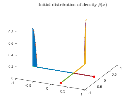
The initial density $\bar{\rho}(x)$ (see Figure 1, right) is defined by the restriction on the network of the function

\bar{\rho}(x_{1},x_{2}):=\max(0,0.65-4\,(x_{1}+1)^{2}-4\,x_{2}^{2},\,0.75-(6\,(x_{1}-0.2))^{2}-(6\,(x_{2}-0.8))^{2}).

The set of the boundary points $V_{b}$ , i.e. the target points, is given by the vertexes in $(0.2,-0.8)$ and $(0.8,0)$ , where $u^{n}$ is imposed equal to zero.

We will consider two possible cases for the boundary conditions (BCs) for the conservation law: the case with a no-flux condition (in such case the mass is conserved inside the network) and the case with a homogeneous Dirichlet condition on the target points (see Remark 4.1). Those BCs are relative to a different choice of the model: the no-flux condition corresponds to target points where the crowd tends to concentrate, for example the stage of a concert, the various points of interest during the annual Hajj, see [4], etc. The homogeneous Dirichlet condition, instead, corresponds to target points which can be seen as exits of large dimensions: any mass touching them exits instantaneously from the network.
First objective of this section is to show the stability of the discrete system: with this aim we consider a first order numerical flux as in (21). The case with a second order correction (stochastic perturbation adding diffusion) is more regular and it will be take into account in the next Test 3.

We perform the simulation fixing the discretization parameter $dx=0.01$ and the time step $dt=0.002$ , hence the stability condition (36) is verified since we observe $\|m\|_{\infty}\leq 1-2\rho\leq 1$ and $dx/(D\,dt)=5/4$ .

Test 1

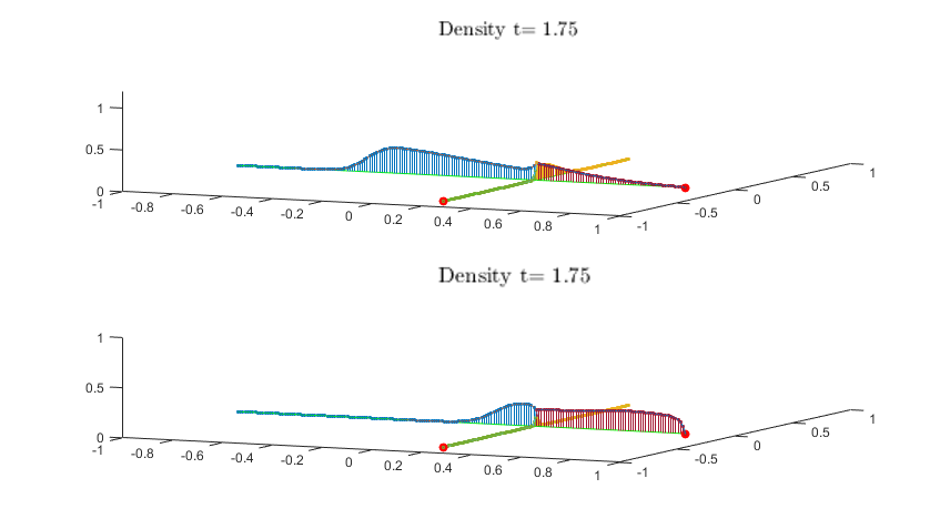
We start considering the case of homogeneous Dirichlet boundary conditions. At the beginning of the simulation, the two initial masses start to move in the direction of the two target points acting as exits. The mass coming from the edge connecting $(0.2,0)$ to $(0.2,0.8)$ has a shorter path so it arrives on the junction node and it turns in direction of the closer exit $(0.8,0)$ (Figure 1). In Figure 2 it is possible to observe the first interaction time between the two masses: the arrival of the mass coming from the edge connecting $(-1,0)$ to $(0.2,0.8)$ produces a congestion near the exit $(0.8,0)$ , therefore the other exit $(0.2,-0.8)$ becomes convenient as it is possible to observe in the graph of the drift potential $u$ , see Figure 3 (below) and compare with Figure 2 (below). Therefore, the exit $(0.2,-0.8)$ attracts a part of the mass (Figure 3 above). This phenomena is peculiar of the Hughes’ model and it has been observed also in other works (see e.g. [19] or [13]). Once reached the target, the mass exits from the network (Figure 3 above, on the exit $(0.8,0)$ ).

Test 2

In a second simulation we compute the same solution with the no-flux boundary condition. In this case, the mass is conserved. The first part of the test shows the same results as above: the masses are attracted by the target point $(0.8,0)$ , but differently the mass starts to concentrate, reducing its speed until the exit $(0.2,-0.8)$ becomes convenient. When also this second target point reaches its maximal value of the density getting congested, the mass reaches a stable configuration (Figure 4). In the case of a coarse time step $dt$ , some oscillatory phenomena are observed in the second part of the test (chattering), where essentially the mass changes alternatively objective between the two target points. With a finer time discretization, those effects are reduced till disappearing. This test confirms even more than the previous case the stability of the discrete system and the fact that the density is always strictly lower than the maximal value 1, even in the extreme case, when we force the mass to concentrate.

Test 3

As last simulation on this network, we add to the conservation law a term of the type (22), which can be interpreted, from a model point of view, as a stochastic perturbation in the motion of the mass and, from an analytic point of view, as a second order regularizing term in the equation. In Figure 5 it is possible to see the effects of the diffusive term: the solution is more regular and congestion is not present. This is a phenomenon observed also in [8]: the presence of a stochastic noise prevents the mass to concentrate over a certain ratio. This has the indirect effect to help the overall evacuation time (i.e. the first time step where the density on the domain is null everywhere) for certain configurations of the system (we can observe this comparing Figure 3 with Figure 5). Avoiding congestion brings also some other macroscopic effects: in this case all the mass is exiting by the more convenient “exit” located in $(0.8,0)$ . Since this arc is not getting congested, the agents do not change strategy using the other “exit” in $(0.2,-0.8)$ .

5.2 A Stadium evacuation test

The stadium at the Wuhan Sports Centre (Fig. 6, left) is a multi-use stadium located in Wuhan, China. Completed in 2002, it was used as test benchmark for mass-evacuation in [14]. The stadium has 42 bleachers (tiers of seats) distributed on all 3 floors and has 9 exits (Fig. 6, right) for evacuation; the capacity declared of the structure is of 54,357 spectators. Transforming a bit the structure (we consider a planar network) the evacuation network in this stadium (Fig. 6, right) has 108 arcs and 63 nodes. After an uniform discretization of the arcs, the number of nodes of the network is around $7\cdot 10^{3}$ with a similar number of connections.

The choice of the initial configuration of density can be variable with respect to the aspect that we want to underline (by choosing a high initial uniform density distribution, we can test the network in an extremely crowded scenario; a random density choice can simulate some not standard cases of anomalous local concentration of crowd, etc). In this test, we chose the following initial datum

\bar{\rho}(x_{1},x_{2}):=\max(0,0.7-0.7x^{2}-0.84y^{2}),

(we always mean the restriction of such function on the network), this distribution in our intention should render the higher concentration of spectators in the areas closer to the court. We approximate uniformly the arcs using the discretization step $dx=0.01$ and we sample the time with $dt=0.002$ . Also in this case the condition (36) is guaranteed (the maximum number of connections per node $D$ is $5$ ) and the scheme is stable. In Figure 7 we can see the initial distribution of the density and the potential driving the individuals toward one of the exits. In Figure 8 it is shown the evolution of the system in various moments. We can notice that, despite the general symmetry of the structure, the behavior is highly conditioned by the position and the number of the exits. Of particular interest is the difference between the evacuation of sectors A/B and C/D (refer to Fig. 6). As it can be seen from the scheme, the sector A is served by only one exit, differently from C, where two exits are present. Analogously, the sector D has 4 exits conversely to sector B which has just two. This brings to an orderly and efficient evacuation in the sectors C/D, with a well balanced use of the exits available. In the other case (sector A/B), the observed dynamics are different: on the paths toward the only three exits, in proximity to some nodes with multiple access, there are the appearance of high density congested regions. We can observe also some of the phenomena discussed previously: reduction of the speed in the congested regions, changes of strategy, doubtful choice between two strategies (chattering). This has the macroscopic effect to rise up the final time necessary to evacuate the regions involved as we can observe in the last samples of Figure 8: the sectors C/D are already empty, the sectors A/B, instead, show congestion and a laborious flow through them. It is interesting to observe that a more efficient (for evacuation purposes) network is not trivially a network with more exits but a structure that avoids to drive big masses of agents to pass at the same time in the same nodes. This is a consequence to the incapacity of the agents represented in the model to forecast the future configuration of the system in order to choose the best strategy to adopt. For those reasons, the model is particularly appropriate to simulate the behavior of a crowd in a known network in presence of unpredicted events (an evacuation order, unusual high concentration in common transport facilities, etc.).

6 Conclusions

In this paper we have presented a discrete Hughes’ model for pedestrian flow on a graph. We have shown that, differently from the analogous continuous model, this discrete model is well-posed for any time $n\in{\mathbb{N}}$ under some natural assumptions on the flux, continuing to share some qualitative properties with the corresponding continuous model, as the interpretation of the solution of the graph eikonal equation as a distance from the boundary, change of strategies, congestion, etc.
Several tests have been shown, analyzing and comparing the results and the behaviors obtained with different conditions (no BCs, homogeneous Dirichlet BCs or adding a diffusive term). The experimental examples have confirmed the validity of the proposed model, showing that the discrete system is always stable, even in the extreme case, when we force the mass to concentrate.

References

[1] A. Alla, M. Falcone, D. Kalise, An efficient policy iteration algorithm for dynamic programming equations, SIAM J. Sci. Comput., 37(1) (2015), A181–A200.
[2] D. Amadori, M. Di Francesco, The one-dimensional Hughes model for pedestrian flow: Riemann-type solutions, Acta Math. Sci., 32(1) (2012), 259–280.
[3] D. Amadori, P. Goatin, M.D. Rosini, Existence results for Hughes’ model for pedestrian flows, J. Math. Anal. Appl., 420(1) (2014), 387–406.
[4] Anonymous, “Jamarat: study of current conditions and means of improvements”, Hajj Research Centre, Um Al-Qura University Saudi Arabia, 1984.
[5] M. Bardi, J.P. Maldonado Lopez, A Dijkstra-type algorithm for dynamic games, Dyn. Games Appl., (2015) 1–14.
[6] N. Bellomo and C. Dogbé, On the modeling of traffic and crowds: a survey of models, speculations, and perspectives, SIAM Rev., 53(3) (2011), 409–463.
[7] M. Briani and E. Cristiani, An easy-to-use algorithm for simulating traffic flow on networks: Theoretical study, Netw. Heterog. Media, 9 (2014), 519–552.
[8] E. Carlini, A. Festa, F.J. Silva and M.T. Wolfram, A Semi-Lagrangian scheme for a modified version of the Hughes model for pedestrian flow http://arxiv.org/abs/1601.07324
[9] F. Camilli and C. Marchi, A comparison among various notions of viscosity solutions for Hamilton-Jacobi equations on networks, J. Math. Anal. Appl., 407 (2013), 112–118.
[10] F. Camilli, A. Festa and D. Schieborn, An approximation scheme for a Hamilton-Jacobi equation defined on a network, Appl. Numer. Math., 73 (2013), 33–47.
[11] G. Costeseque, J.P. Lebacque and R. Monneau, A convergent scheme for Hamilton-Jacobi equations on a junction: application to traffic, Numer. Math., 129(3) (2015), 405–447.
[12] E. Cristiani and F.S. Priuli, A destination-preserving model for simulating Wardrop equilibria in traffic flow on networks, Netw. Heterog. Media, 10 (2015), 857–876
[13] M. Di Francesco, P.A. Markowich, J.F. Pietschmann and M.T. Wolfram, On the Hughes’ model for pedestrian flow: the one-dimensional case, J. Differential Equations, 250(3) (2011), 1334–1362.
[14] Z. Fang, Q. Li, Q. Li, L. D. Han and D. Wang, A proposed pedestrian waiting-time model for improving space-time use efficiency in stadium evacuation scenarios, Build. Environ., 46 (2011), 1774–1784.
[15] M. Garavello and B. Piccoli, “Traffic Flow on Networks” AIMS Series on Applied Mathematics, Vol. 1, American Institute of Mathematical Sciences, 2006.
[16] L. Huang, S.C. Wong, M. Zhang, C.W. Shu, and W.H.K. Lam, Revisiting Hughes’ dynamic continuum model for pedestrian flow and the development of an efficient solution algorithm, Transportat. Res. B-Meth., 43 (2009), 127–141
[17] R.L. Hughes, The flow of large crowds of pedestrians, Math. Comput. Simulat., 53 (2000), 367–370.
[18] R.L. Hughes, A continuum theory for the flow of pedestrians, Transport. Res. B-Meth., 36(6) (2002), 507–535.
[19] R. L. Hughes, The flow of human crowds, Annu. rev. fluid mech., 35(1) (2003), 169–182.
[20] J. Manfredi, A. Oberman and A. Sviridov, Nonlinear elliptic Partial Differential Equations and p-harmonic functions on graphs, Differ. Integral Equ. 28 (2015), 79–102.
[21] M. Puterman and S.L. Brumelle, On the convergence of policy iteration in stationary dynamic programming, Math. Oper. Res., 4(1) (1979), 60–69.
[22] J.D. Towers, Convergence of a difference scheme for conservation laws with a discontinuous flux, SIAM J. Numer. Anal., 38(2) (2000), 681–698.
[23] A. Treuille, S. Cooper and Z. Popovîc, Continuum Crowds, ACM Trans. Graph., 25 (2006), 1160–1168.