Dispersive thermometry with a Josephson junction coupled to a resonator
Abstract
We have embedded a small Josephson junction in a microwave resonator that allows simultaneous dc biasing and dispersive readout. Thermal fluctuations drive the junction into phase diffusion and induce a temperature-dependent shift in the resonance frequency. By sensing the thermal noise of a remote resistor in this manner, we demonstrate primary thermometry in the range from 300 mK to below 100 mK, and high-bandwidth (7.5 MHz) operation with a noise-equivalent temperature of better than 10 . At a finite bias voltage close to a Fiske resonance, amplification of the microwave probe signal is observed. We develop an accurate theoretical model of our device based on the theory of dynamical Coulomb blockade.
I Introduction
An apparently simple coupled system of an ultrasmall Josephson junction and a transmission line resonator exhibits very rich physics which currently attracts a lot of attention. It has been known for a long time that the current voltage characteristics of such a junction is described by well-developed theory [1, 2, 3], which emphasizes the effect of the electro-magnetic environment on the fluctuations of the Josephson phase. This theory has been experimentally verified, see e.g. in Refs. 4, 5, 6. In more recent experiments, the ”bright side” effect, i.e., emission of radiation by the junction into the transmission line, has been detected [7], and the signs of lasing by a single Cooper pair box into a resonator have been observed [8]. The experiments have stimulated a series of theory papers that describe, for example, non-linear quantum dynamics of the system [9, 10], emission of entangled photons in two separate resonators [11], antibunching of the emitted photons [12], and the full quantum theory of emitted radiation [13].
In this Letter, we demonstrate that depending on bias condition an ultrasmall Josephson junction can operate either as a sensitive noise detector or as a source of photons. We weakly couple the resonator to the outer transmission line and monitor its resonance frequency and the quality factor via microwave reflection measurements. We show that at zero bias the shift of the resonance frequency is inversely proportional to temperature and the junction operates as an ultra-sensitive thermometer and noise detector. In this regime we effectively realize a power-to-frequency transducer. Applying bias voltage to the junction we detect amplification of the probe signal close to the resonance condition, where the Josephson frequency matches the fundamental frequency of the resonator . In this case the junction may operate as an amplifier or as a source of radiation. We also develop a high-frequency generalization of the -theory and show that it describes the experiment fairly well in the whole range of bias voltages studied. Our results hilight the unique properties of an ultrasmall Josephson junction and outline future applications as a thermometer or as a general-purpose radiation and noise detector. In particular, we estimate that a thermal photodetector based on this method of temperature sensing could reach photon-resolving energy resolution in the microwave domain.

II Overview of the experiment
II.1 Sample design
We have fabricated a small Josephson junction and coupled it to a coplanar waveguide (CPW) resonator that allows simultaneous dc biasing and microwave probing [Fig. 1(a),(b)]. The chip layout and the design philosophy of microwave elements mirror those of superconducting quantum processors [14]. In the absence of Josephson dynamics, the fundamental resonance mode is characterized by the resonance frequency GHz, the internal and coupling quality factors and , respectively, and impedance , where is the characteristic impedance of the waveguide. The Josephson element was realized as a planar tunnel junction between an aluminum electrode and a 1 m long proximitized Al/Cu/Al SNS wire [Fig. 1(c)]. A separate heater line allows local Joule heating of the wire to aid in characterization. Earlier experiments on resonator-coupled tunnel junction structures have employed thermometry based on quasiparticle transport [15], and an initial observation of supercurrent thermometry was reported in Ref. 16. Details of device fabrication, measurement setup, and microwave readout are presented in the supplement [18].
The sample chip contains another similar device with the resonator 1 GHz lower in frequency. The two device structures can be independently dc biased and read out by frequency multiplexing, and they showed similar behavior in the experiments. Here, we mainly discuss the higher-frequency device whose readout resonance had smaller intrinsic loss.
II.2 Theory
The junction dynamics is described by the equation
| (1) |
where is the Fourier transformed admittance of the electromagnetic environment surrounding the junction and including junction capacitance [see Fig. 1(d)], is the impedance of the environment, is the Josephson current and is the current induced by the probe signal. If the junction critical current, , is high, one should put in Eq. (1). However, here we consider the limit in which case, applying the theory developed in Refs. 17, we find (see the Supplement [18] for details)
| (2) | |||||
Here, is the high frequency component of the Josephson phase induced by the combined effect of the probe signal and the resonator. The functions and characterize the environment and are defined as follows
| (3) |
In these expressions, is the spectral density of voltage fluctuations across the junction and is an infinitely small positive constant. In equilibrium, the fluctuation-dissipation theorem is valid and one finds . In our experiment, the impedance is dominated by transmission line resonator [see Figs. 1(a) and (d)], and can be formally written as
| (4) |
where is the angular frequency of the fundamental () resonance, and is the damping rate of the th harmonic mode. One has , where is the internal damping and originates from coupling to the outer transmission line. In the experiment, contributions from up to the second harmonic () can be observed.
II.3 Linearized treatment
Linearizing the problem in , we introduce the impedance of the junction
| (5) |
where the function
| (6) |
characterizes the high frequency response of the electromagnetic environment and generalizes the familiar function. The latter describes only the DC properties of the junction, i.e., its - curve. The two functions are related as . Taking the limit and making use of the small- assumption, we find the modified resonance frequency and the internal damping rate of the fundamental resonance () as
| (7) | |||||
| (8) |
III Zero-bias operation

At low bias voltages and in the limit of small-signal microwave probing, the voltage dependence of the resonance frequency reduces to a simple Lorentzian form
| (9) |
where denotes effective low frequency shunt resistance, and the other parameters are
, and . To arrive at Eq. (9), we have assumed , and the limit of classical phase fluctuations k. Both conditions are satisfied in our experiment.
In the experiment, the resonance line displays a clear temperature [Fig. 2(c)] and bias dependence. In Fig. 2(a) we analyze the experimental low-bias part of frequency-voltage dependence, which indeed has the Lorentzian form. The width of the Lorentzian is proportional to temperature at mK [Fig. 2(b)]. Comparing the experimental temperature dependence of the width with Eq. (9), we determine the low frequency shunt resistance . By design, the shunt resistance is given by the external bias resistor (nominally 50 ) plus any effective in-line dc resistance including the SNS wire and contacts ( for Cu in normal state). The deviation from the linear dependence at lowest temperatures is due to two independent mechanisms. When the condition is violated, our model no longer applies and a supercurrent feature with a width close to emerges instead. Besides this, insufficient thermalization can result in saturation of sample temperature. With the linear scaling established earlier, the minimum observed width corresponds to a temperature of 44 mK [20].
One can similarly work out the approximate form of the quality factor at low bias voltage. The result reads
| (10) |
Here we assumed that the thermal linewidth significantly exceeds the damping rate of the fundamental resonance [18]. This condition is satisfied in our experiment.
IV Finite-voltage resonances
In Figs. 3(a), (b) we show, respectively, the resonance frequency, , and the internal quality factor, , as a function of the bias voltage applied to the junction. The experimental data are fitted with the temperature-dependent critical current as the only free parameter. (Refer to Supplement for comparison of values determined with different methods, and for theory expressions covering full bias range [18]). It is interesting that the internal quality factor becomes negative at bias voltages close to and at a sufficiently low temperature [Fig. 3(c)]. In this regime the junction pumps energy into the resonator and amplifies the probe signal. Previously emission from the junction has been detected under similar conditions [7]. The theory predicts that the internal damping becomes negative at and for bias voltages in the range
| (11) |
Taking nA we estimate the threshold temperature to be mK. Experimentally, the threshold temperature lies between 120 and 170 mK based on data shown in Fig. 3(b). Although the condition indicates the generation of microwave power by the junction, it does not imply in the two-port feedline configuration employed in our experiment. For that, a stricter condition needs to be met, which occurs theoretically at mK and was not realized in the experiment. In earlier work [21], a one-port device based on this principle has been operated as a reflection amplifier at 2.8 GHz.
V Non-linear operation
V.1 High-power readout

Here, we relax the assumption to describe the response to strong microwave probing. High-power probing is relevant for optimizing the noise-equivalent temperature, although overheating of the sample can impose a stricter limit to probing power than the non-linearity of Josephson dynamics. In a two-port feedline configuration employed in the experiment, the amplitude of high-frequency phase modulation is related to the incident probe power at probe frequency as
| (12) |
where . Denoting by and the power-dependent expressions for the resonance frequency and internal quality factor, respectively, we find the relations
| (13) | |||||
| (14) |
where the are Bessel functions of the first kind, and the small-signal and are evaluated according to Eqs. (4) and (5), respectively. An experimental power sweep performed at zero bias and at the base temperature of the cryostat (13 mK) [Fig. 4(a)] indeed reveals Bessel-type oscillations of the resonance frequency. Solution of the circuit model with -dependent and reproduces the data well [Fig. 4(b)] including fine structure that appears with off-resonant probing at large power.
The non-linearity of the model can result in multi-valued solutions for certain combinations of low temperature, large , and large probing power. We did not observe hysteretic or bistable behavior in the experiment. Physically, it is likely that large probing power locally heats up parts of the sample or the surrounding circuitry, raising the effective temperature. It is in principle possible to include a thermal balance in the model and solve it in a self-consistent manner. Here, we explain the high-power response by using a constant elevated temperature (75 mK) throughout the simulation. Good agreement with the constant-temperature simulation shows that the present design is not severly overheated even at dBm incident probing power.
V.2 Local heating
In an indealized desription of our device, the Josephson element does not have an internal temperature of its own. Instead, the observed temperature dependence stems from fluctuations of the electromagnetic environment. Localized Joule heating or electronic cooling of the SNS wire will generally drive the system to a quasi-equilibrium state with independent electron and environment temperatures [25]. We demonstrate sensitivity to the local electron temperature by modulating the wire temperature with either CW microwave heating, or by voltage biasing the other tunnel junction that was otherwise unused in the experiment (data shown in the Supplement [18]). The data is consistent with a model where the cryostat sets the temperature of electromagnetic environment by thermalizing the cold bias resistor, and the wire temperature is probed through its effect on the of the junction. Here, the temperature dependence follows from that of proximity superconductivity in diffusive metallic weak links [26]. Optimized detectors based on this mode of operation have been explored in detail in earlier works by Govenius et al. [27].
VI Sensitivity and noise
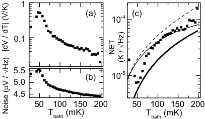
To evaluate the suitability of this thermometer for calorimetric and bolometric experiments [28], we characterize the sensitivity of the temperature readout with continuous wave (CW) microwave probing at zero bias with phase-sensitive heterodyne readout. Despite conceptual similarities with noise thermometry employing SQUID readout [29], our device indicates temperature directly through a change in the phase of the probe signal instead of relying on power detection with room-temperature electronics. To scan rapidly the parameter space of possible combinations of probing frequency and power, we studied the single-shot detection fidelity of discrete heating pulses (1 s duration, 0.8 pW nominal power) using only the thermometer readout. An optimum was found at 5.671 GHz, nominal 118 dBm power incident at the sample box. Next, during a bath temperature sweep up to 200 mK, we recorded the CW quadrature voltage amplitudes , and the full noise spectrum of the quadrature readout. We evaluate numerically the voltage responsivity corresponding to homodyne detection with optimal phase [Fig. 5(a)]. Similarly, the NET for homodyne detection is , where is the voltage noise level in one quadrature [Fig. 5(b), (c)]. Using the small-signal theory and sample parameters determined earlier, we can reproduce the observed NET values for temperatures higher than 75 mK. We have included the responsivity enhancement from weak temperature dependence of in the model. Comparing the results to a calculation with , we find that inductance and noise contributions to responsivity are equal at 200 mK, with the inductance modulation losing its significance below 100 mK. For the theoretical NET calculation, we have assumed a total power loss of 11 dB from cabling between generator output and the cold amplifier, and amplifier-limited system noise with K (as per preamplifier specifications). These quantities cannot be independently determined within a linearized model. The origin of the temperature dependent component of readout noise that follows the shape of the responsitivity curve is unknown. The low frequency resonator was measured simultaneously in an identical manner and the noise level was found to be constant within 0.5%. We estimate the power dissipated at the sample (, including shunt resistors) as , where is the incident probing power and , using modeled values for and . The loss fraction is smaller than 0.5 at all temperatures, resulting in total dissipation less than 0.8 fW [22]. Finally, using the theory for high-power readout presented in Sec. V.1, we evaluate the lowest achievable NET when overheating of the sample is neglected [Fig. 5(c), thick line].
VII Outlook
Small power dissipation, sub-s temporal resolution, and good sensitivity at sub-100 mK temperatures make this type of a themometer a promising candidate for calorimetric experiments [28]. In a nano-calorimeter implementation [16], the external macroscopic bias resistor would be replaced with a metallic or semiconducting nanowire with similar resistance but minimal volume. In a calorimeter device, it is critical to consider the tradeoff between the thermometer sensitivity and the power dissipation induced by the thermometer readout. One can formalize this tradeoff by writing the noise-equivalent temperature (NET, units ) explicitly in terms of . For a dispersive thermometer, the general result
| (15) |
follows from linearized circuit theory assuming one-port reflection measurement and readout noise that is described by the system noise temperature . As long as the responsivity does not explicitly depend on , the choice is optimal. For a pure reflection measurement, this implies = at resonance. It is possible to derive simple expressions describing our Josephson thermometer by substituting the linear-response formulas of Eqs. (9) and (10) with and assuming . One has
| (16) |
to the first order in . Working from the above relation, one can estimate the expected energy resolution of a calorimeter under quite general assumptions (see Appendix A for details) about the temperature dependence of the heat capcity () and the thermal link of the calorimeter platform () as
| (17) |
Note that the validity of Eq. (9) requires the fraction to be larger than . For a practical example, we consider a small metallic absorber (, ) on a suspended platform with quantized phononic heat conductance (, see Ref. 29) at a temperature of 20 mK, microwave probe at GHz, and a readout chain approaching the standand quantum limit , which results in an estimated energy resolution of .
In conclusion, we have constructed a power-to-frequency transducer based on a small Josephson junction and demonstrated sensitive high-bandwidth thermometry at sub-100 mK temperatures. We have also developed a theoretical model based on strong environmental fluctuations that describes the measurements within its expected range of validity. Good performance and versatility of the approach suggest it can find use in a wide range of experiments requiring sensitive thermometry, calorimetry, or noise detection. Our results also hint at the possibility of further performance gains in designs with large and/or , whose analysis, however, requires an improved theoretical model.
Acknowledgements.
This work was funded through Academy of Finland grants no. 2722195, 284594, and 285300. We acknowledge the availability of the facilities and technical support by Otaniemi research infrastructure for Micro and Nanotechnologies (OtaNano), and VTT technical research center for sputtered Nb films. M.Z. thanks the EAgLE project. K.L.V. acknowledges financial support from Jenny and Antti Wihuri foundation. We thank A. Savin for the dilution refrigerator setup.Appendix A Calorimeter optimization
We consider a generic calorimeter platform that is described by the model equations
subject to steady-state thermal balance
| (18) |
where and denote the temperature of the calorimeter and its surrounding thermal bath, respectively, is the energy resolution, is the heat capacity of the calorimeter, is its linearized heat coductance at the operation point, describes the steady-state heat flow between the calorimeter and its surroundings, and , are numbers and and numerical constants describing the thermal properties of the calorimeter, and describes the sensitivity of the thermometer as function of the steady-state dissipation and . The choice of the readout power (or, equivalently, ) influences the steady-state operation tempeature , and, consequently, through the temperature dependence of and .
If one furthermore has
| (19) |
with a numerical constant and a number, the problem can be solved through the introduction of a Lagrange multiplier. Note that Eq. (16) describing our thermometer is of this form. One finds
| (20) |
and
| (21) |
where the superscript denotes quantities calculated at the optimum steady-state operation point. In practice, one can evaluate Eq. (21) with to approximate the energy resolution, as the optimal probing power does not raise the absorber temperature significantly.
References
- [1] D.V. Averin, Yu.V. Nazarov, A.A. Odintsov, Physica C 165-166, 945 (1990).
- [2] G. L. Ingold and Yu.V. Nazarov, in Single Charge Tunneling, edited by H. Grabert and M. H. Devoret, NATO ASI, Ser. B (Plenum, New York, 1992), Vol. 294, p. 21.
- [3] G.L. Ingold, H. Grabert, U. Eberhardt, Phys. Rev. B 50, 395 (1994).
- [4] T. Holst, D. Esteve, C. Urbina, and M.H. Devoret, Phys. Rev. Lett. 73, 3455 (1994).
- [5] A. Steinbach et al., Phys. Rev. Lett. 87, 137003 (2001).
- [6] Yu. A. Pashkin et al., Phys. Rev. B 83, 020502 (2011).
- [7] M. Hofheinz et al., Phys. Rev. Lett. 106, 217005 (2011).
- [8] F. Chen et al., Phys. Rev. B 90, 020506(R) (2014).
- [9] V. Gramich, B. Kubala, S. Rohrer, and J. Ankerhold, Phys. Rev. Lett. 111, 247002 (2013).
- [10] B. Kubala, V. Gramich, and J. Ankerhold, Phys. Scr. T165, 014029 (2015).
- [11] A. D. Armour, B. Kubala, and J. Ankerhold, Phys. Rev. B 91, 184508 (2015).
- [12] J. Leppäkangas et al., Phys. Rev. Lett. 115, 027004 (2015).
- [13] J. Leppäkangas, M. Fogelström, M. Marthaler, and G. Johansson, Phys. Rev. B, 93, 014506 (2016).
- [14] A. Wallraff et al., Nature, 431, 162 (2004). M. Jerger et al., Appl. Phys. Lett. 101, 042604 (2012). J. P. Groen et al., Phys. Rev. Lett., 111, 090506 (2013).
- [15] M. Nahum and J. M. Martinis. Appl. Phys. Lett. 66, 3203 (1995). S. Gasparinetti et al., Phys. Rev. Applied 3, 014007 (2015).
- [16] K. L. Viisanen et al., New. J. Phys 17, 055014 (2015).
- [17] U. Eckern, G. Schön, and V. Ambegaokar, Phys. Rev. B 30, 6419 (1984). G. Schön and A.D. Zaikin, Phys. Rep. 198, 237 (1990).
- [18] Supplemental Material.
- [19] Weak flux modulation with a global coil was observed. For the higher, more sensitive resonator, the peak-to-peak amplitude was 2 MHz at zero bias. In all subsequent experiments, flux setting for the largest frequency shift was used.
- [20] Fitting the base temperature data with two superimposed Lorentzians, located symmetrically around zero bias, yields a broadening corresponding to 31 mK.
- [21] P. Lähteenmäki et al., Sci Rep. 2, 276 (2012).
- [22] Cabling losses on the input side are not included, and would diminish the estimated dissipation proportionally.
- [23] M. Nahum, T. M. Eiles, and J. M. Martinis, Appl. Phys. Lett, 65, 3123 (1994).
- [24] M. M. Leivo, J. P. Pekola, and D. V. Averin, Appl. Phys. Lett. 68, 1996 (1996).
- [25] F. Giazotto et al., Rev. Mod. Phys. 78, 217 (2006).
- [26] P. Dubos et al., Phys. Rev. B 63, 064502.
- [27] J. Govenius et al., Phys. Rev. B 90, 064505 (2014), Phys. Rev. Lett. 117, 030802 (2016).
- [28] Here, we refer to an experimental setting where radiation is coupled to a small absorber, and the thermometer is used to monitor the absorber temperature.
- [29] K. Schwab, E. A. Henriksen, J. M. Worlock, and M. L. Roukes, Nature 404, 974-977 (27 April 2000).