Channel Estimation for mmWave Massive MIMO Based Access and Backhaul in Ultra-Dense NetworkThanks: This work was supported in part by the International Science & Technology Cooperation Program of China (Grant No. 2015DFG12760), the National Natural Science Foundation of China (Grant Nos. 61571270 and 61271266), the Beijing Natural Science Foundation (Grant No. 4142027), and the Foundation of Shenzhen government.

It has been the consensus that future 5G networks should achieve the 1000-fold increase in system capacity [2, 1, 3]. To realize such an aggressive 5G version, millimeter-wave (mmWave) massive MIMO used for the access and backhaul in ultra-dense network (UDN) has been considered as a promising technique to enable gigabit-per-second user experience, seamless coverage, and green communication [2]. In this paper, we consider the heterogeneous network (HetNet) with the separation of control plane and data plane, as shown in Fig. 1. For such an HetNet, the macrocell base station (BS) provides the control signaling service for the large coverage area using conventional low frequency band, while the ultra-dense small BSs are specialized in data resources with limited coverage area for high-rate transmission, where the emerging mmWave massive MIMO technique is exploited for the access and backhaul [2, 4]. Moreover, the centralized radio access network (C-RAN) architecture can be integrated into the HetNet for the improved physical layer transmission, handover, scheduling, and etc., where the ultra-dense small cells are regarded as the remote ratio head (RRH) and macrocell BS is considered as the baseband unit (BBU).

Due to the ultra-dense deployment, each user may receive the signal from multiple RRHs. To exploit the advantages of C-RAN architecture, the accurate channel state information (CSI) associated with multiple RRHs known at BBU is essential for the joint beamforming, scheduling, and cooperation among the ultra-dense small-cell BSs. However, how to require the reliable channel estimation with low overhead can be challenging, since the pilot overhead to estimate the channels associated with a large number of antennas in mmWave massive MIMO can be prohibitively high [5]. [6, 7] have proposed a multilevel codebook based joint channel estimation and beamforming for mmWave access and backhaul. However, this scheme only considers the mmWave multi-antenna systems with analog beamforming, which is limited to the point-to-point based single-stream transmission. To solve this problem, the mmWave massive MIMO has been emerging [8, 2, 9, 10], where the hybrid analog-digital beamforming scheme is proposed to support the multi-stream transmission with low hardware cost and energy consumption. In [9], an adaptive channel estimation has been proposed for mmWave massive MIMO. However, this scheme is limited to the single-cell scenario. Besides, [10] has proposed the reference signal design for the channel estimation in mmWave massive MIMO. However, the scheme fails to exploit the sparsity of mmWave channels, which may lead to a certain performance loss.

Recent study and experiments have shown that the mmWave massive MIMO channels appear the obviously sparsity in the angular domain [2, 9], since the path loss for non-line-of-sight (NLOS) paths is much larger than that for line-of-sight (LOS) paths in mmWave [11, 12]. Moreover, since the spatial propagation characteristics of the mmWave channels within the system bandwidth are nearly unchanged, such sparsity is shared by subchannels of different subcarriers when the widely used orthogonal frequency-division multiplexing (OFDM) is considered. This phenomenon is referred to as the spatially common sparsity within the system bandwidth [13]. In this paper, we first propose the non-orthogonal pilot design at the small-cell BSs used for channel estimation. Furthermore, we propose a structured compressive sensing (SCS)-based sparse channel estimation scheme at the receiver to estimate the channels for the mmWave massive MIMO in UDN. Simulation results verify that the proposed scheme is superior to its counterpart, and it is capable of approaching the performance bound with low overhead.

Throughout our discussions, the boldface lower and upper-case symbols denote column vectors and matrices, respectively. The Moore-Penrose inversion, transpose, and conjugate transpose operators are given by $(\cdot)^{{\dagger}}$, $(\cdot)^{\rm T}$ and $(\cdot)^{*}$, respectively, while $\lceil\cdot\rceil$ is the integer ceiling operator. $(\cdot)^{-1}$ is the inverse operator. The $\ell_{0}$-norm and $\ell_{2}$-norm are given by $\|\cdot\|_{0}$ and $\|\cdot\|_{2}$, respectively, and $\left|\Gamma\right|$ is the cardinality of the set $\Gamma$. The support set of the vector $\mathbf{a}$ is denoted by ${\rm supp}\{\mathbf{a}\}$. The rank of ${\bf A}$ is denoted by ${\rm rank}\{{\bf A}\}$, while ${\rm E}\{\cdot\}$ is the expectation operator. $\left({\bf a}\right)_{\Gamma}$ denotes the entries of $\mathbf{a}$ whose indices are defined by $\Gamma$, while $\left({\bf A}\right)_{\Gamma}$ denotes a sub-matrix of $\mathbf{A}$ with column indices defined by $\Gamma$. $\otimes$ is the Kronecker product and ${\rm{vect}}\left({\cdot}\right)$ is the vectorization operation according to the columns of the matrix. $\left[{\bf a}\right]_{i}$ denotes the $i$th entry of the vector $\mathbf{a}$, and $\left[{\bf A}\right]_{i,j}$ denotes the $i$th-row and $j$th-column element of the matrix $\mathbf{A}$.

Conventionally, mmWave is considered to be not suitable for access due to its high path loss, Moreover, the signal-to-noise-ratio (SNR) before beamforming is conventionally considered to be low due to the high path loss, which leads to the challenging channel estimation in mmWave communications. However, for the UDN scenarios, we will clarify this misunderstanding by comparing the path loss in UDN working at 30 GHz and that in conventional cellular networks working at 3 GHz. Specifically, considering the multipath fading, signal dispersion, and other loss factors, the path loss component of Friis equation in decibel (dB) can be provided as [6],

where $f_{c}$ (MHz) is the carrier frequency, $\alpha$ (dB/km) is the path loss exponent, $d$ (km) is the link distance, ${\alpha_{o}}$ (dB/km) is the atmospheric attenuation coefficient, and ${\alpha_{r}}$ (dB/km) is the rain attenuation coefficient. For the conventional cellular systems with $f_{c}=3$ GHz and $d=1$ km for example, we have $\eta=192.62$ dB, where $\alpha=2.2$ dB/km is considered in urban scenarios [6], and the atmospheric attenuation and rain attenuation are ignored. By contrast, for UDN with $f_{c}=30$ GHz, we have $\eta=188.27$ dB with $d=100$ m for backhaul link and $\eta=161.78$ dB with $d=30$ m for access link, where $\alpha=2.2$ dB/km, $\alpha_{o}=0.1$ dB/km, and $\alpha_{r}=5$ dB/km when the heavy rain with 25 mm/h is considered [1]. Due to the short link distance, the path loss in mmWave is even smaller than that in conventional cellular networks, which indicates the appropriate SNR for channel estimation in the mmWave access and backhaul even before beamforming.

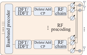
On the other hand, mmWave massive MIMO has been emerging as the promising technique for access and backhaul [8, 2, 9, 10]. For the mmWave massive MIMO, as shown in Fig. 2, the number of baseband chains is larger than one but far smaller than that of the employed antennas, and the hybrid analog and digital beamforming can be exploited for the improved spatial multiplexing with low hardware cost and energy consumption. However, the large number of antennas lead to the challenging issue of channel estimation. Particularly, the delay-domain mmWave massive MIMO channel can be modeled as [6]

where $L$ is the number of multipath, $\tau_{l}$ is the delay of the $l$th path, $N_{T}$, $N_{R}$ are the numbers of antennas at the transmitter and receiver, respectively, and ${{\bf{H}}^{d}_{l}}\in{\mathbb{C}^{{N_{R}}\times{N_{T}}}}$ is given by

with that ${{\alpha_{l}}}$ is the complex gain of the $l$th path, ${{\theta_{l}}}\in[0,2\pi]$ and ${{\varphi_{l}}}\in[0,2\pi]$ are azimuth angles of arrival or departure (AoA/AoD) if we consider the uniform linear array (ULA). In addition, ${{\bf{a}}_{R}}\left({{\theta_{l}}}\right)={\left[{1,{e^{j2\pi d\sin({\theta_{l}})/\lambda}},\cdots,{e^{j2\pi({N_{T}}-1)d\sin({\theta_{l}})/\lambda}}}\right]^{\rm{T}}}$ and ${{\bf{a}}_{T}}\left({{\varphi_{l}}}\right)={\left[{1,{e^{j2\pi d\sin({\varphi_{l}})/\lambda}},\cdots,{e^{j2\pi({N_{R}}-1)d\sin({\varphi_{l}})/\lambda}}}\right]^{\rm{T}}}$ are steering vectors at the receiver and transmitter, respectively, where $\lambda$ and $d$ are wavelength and antenna spacing, respectively.

Since the path loss for NLOS paths is much larger than that for LOS paths in mmWave, the mmWave channels appear the obviously sparsity in the angular domain. Here we consider frequency-domain subchannel ${{\bf{H}}^{f}_{n}}$ ($1\leq n\leq N$) at the $n$th subcarrier, where $N$ is the size of the OFDM symbol, and the relationship between the frequency-domain channel ${{\bf{H}}^{f}_{n}}$ and the delay-domain channel ${\bf{H}}^{d}(\tau)$ has been illustrated in our recent paper [13]. Moreover, we can obtain the sparse channel matrix in the angular domain ${{\bf{H}}^{a}_{n}}$ as [9]

where ${{\bf{A}}_{T}}\in\mathbb{C}^{N_{T}\times N_{T}}$ and ${{\bf{A}}_{R}}\in\mathbb{C}^{N_{R}\times N_{R}}$ are the discrete Fourier transformation (DFT) matrices by quantizing the virtual angular domain with the resolutions of $2\pi/N_{T}$ at the transmitter and $2\pi/N_{R}$ at the receiver, respectively. By vectorizing ${{\bf{H}}^{f}_{n}}$, we can further obtain

where ${\bf{A}}=\left({({{\bf{A}}_{T}^{*})}^{\rm{T}}\otimes{\bf{A}}_{R}}\right)$ and ${{\bf{h}}^{a}_{n}}={\rm{vect}}\left({{{{\bf{H}}}^{a}_{n}}}\right)$. Due to the sparsity of ${\bf h}_{n}^{a}$, we can obtain that

where $\Theta_{n}$ is the support set, and $S_{a}$ is the sparsity level in the angular domain. Note that if we consider the quantized AoA/AoD with the same resolutions as ${\bf{A}}_{T}$ and ${\bf{A}}_{R}$, we have $S_{a}=L$ [9]. Since the spatial propagation characteristics of the channels within the system bandwidth are almost unchanged, $\left\{{\bf h}^{a}_{n}\right\}_{n=1}^{N}$ have the common sparsity, namely,

which is referred to as the spatially common sparsity within the system bandwidth.

In this section, we propose the SCS-based channel estimation scheme for access in UDN, which can be also used to estimate the channels for backhaul. The procedure of the proposed channel estimation and the associated processing is first summarized. Step 1: Under the control of the macrocell BS, several continuous time slots are specialized for channel estimation, where ultra-dense small-cell BSs (RRH) transmit non-orthogonal pilots. Step 2: The user uses the proposed SCS-based channel estimator to acquire the channels associated with multiple small cells nearby. Step 3: The estimated channels are first quantized and then fed back to the macrocell (BBU) for the centralized processing including the beamforming, scheduling, cooperation, and etc.

Due to the hybrid transceiver structure as shown in Fig. 2, we consider each user employs $N_{a}^{\rm{US}}$ antennas and $N_{\rm BB}^{\rm{US}}$ baseband chains with $N_{a}^{\rm{US}}\gg N_{\rm BB}^{\rm{US}}$, while each small-cell has $N_{a}^{\rm{BS}}$ antennas and $N_{\rm BB}^{\rm{BS}}$ baseband chains with $N_{a}^{\rm{BS}}\gg N_{\rm BB}^{\rm{BS}}$. Each user can receive the signal from $M$ small-cell BSs nearby. In downlink channel estimation for one user, the received pilot signal at the $\xi_{p}$th ($1\leq p\leq P$) subcarrier in the $t$th time slot can be expressed as

where ${\bf{r}}_{p}^{(t)}\in\mathbb{C}^{N_{\rm{BB}}^{\rm US}\times 1}$ is the received signal dedicated to the $p$th pilot subcarrier in the $t$th time slot, ${\bf{Z}}_{p}^{(t)}={\bf{Z}}_{{\rm{RF}},p}^{(t)}{\bf{Z}}_{{\rm{BB}},p}^{(t)}\in\mathbb{C}^{N_{a}^{\rm US}\times N_{\rm BB}^{\rm US}}$ is the combining matrix at the receiver with ${\bf{Z}}_{{\rm{BB}},p}^{(t)}\in\mathbb{C}^{N_{\rm BB}^{\rm US}\times N_{\rm BB}^{\rm US}}$ and ${\bf{Z}}_{{\rm{RF}},p}^{(t)}\in\mathbb{C}^{N_{a}^{\rm US}\times N_{\rm BB}^{\rm US}}$ the baseband and RF combining, respectively, ${{\bf{\tilde{H}}}_{p,m}^{f}}={\bf{H}}_{{\xi_{p}},m}^{f}$ and ${{\bf{\tilde{H}}}_{p,m}}^{a}={\bf{H}}_{{\xi_{p}},m}^{a}$ are frequency-domain and angular-domain channel matrices associated with the $p$th pilot subcarrier from the $m$th small-cell BS, respectively, $\Omega_{\xi}=\left\{\xi_{1},\xi_{2},\cdots,\xi_{P}\right\}$ is the index set of the pilot subcarriers, $\xi_{p}$ for $1\leq p\leq P$ denotes the subcarrier index dedicated to the $p$th pilot subcarrier, ${\bf{f}}_{p,m}^{\left(t\right)}={\bf{F}}_{{\rm{RF}},p}^{\left(t\right)}{\bf{F}}_{{\rm{BB}},p}^{\left(t\right)}{\bf{s}}_{p}^{\left(t\right)}\in\mathbb{C}^{N_{a}^{\rm BS}\times 1}$ is the pilot signal transmitted by the $m$th small-cell BS, with ${\bf{F}}_{{\rm{RF}},p}^{\left(t\right)}\in\mathbb{C}^{N_{a}^{\rm BS}\times N_{\rm BB}^{\rm BS}}$, ${\bf{F}}_{{\rm{BB}},p}^{\left(t\right)}\in\mathbb{C}^{N_{\rm BB}^{\rm BS}\times N_{\rm BB}^{\rm BS}}$, ${\bf{s}}_{p}^{\left(t\right)}\in\mathbb{C}^{N_{\rm BB}^{\rm BS}\times 1}$ the RF precoding, baseband precoding, and training sequence, respectively, and ${\bf{v}}_{p}^{(t)}$ is the additive white Gaussian noise (AWGN) at the user. Moreover, (8) can be simplified as

where ${\bf{\bar{H}}}_{p}^{a}=\left[{{\bf{\tilde{H}}}_{p,1}^{a},{\bf{\tilde{H}}}_{p,2}^{a},\cdots,{\bf{\tilde{H}}}_{p,M}^{a}}\right]\in\mathbb{C}^{N_{a}^{\rm US}\times MN_{a}^{\rm BS}}$, ${\bf{\bar{A}}}_{T}^{*}={\rm{diag}}\left\{{{\bf{A}}_{T}^{*},{\bf{A}}_{T}^{*},\cdots,{\bf{A}}_{T}^{*}}\right\}\in\mathbb{C}^{MN_{a}^{\rm BS}\times MN_{a}^{\rm BS}}$, ${\bf{\bar{f}}}_{p}^{\left(t\right)}={\left[{{{\left({{\bf{f}}_{p,1}^{(t)}}\right)}^{\rm{T}}},{{\left({{\bf{f}}_{p,2}^{(t)}}\right)}^{\rm{T}}},\cdots,{{\left({{\bf{f}}_{p,M}^{(t)}}\right)}^{\rm{T}}}}\right]^{\rm{T}}}\in\mathbb{C}^{MN_{a}^{\rm BS}\times 1}$, ${\bf{\bar{h}}}_{p}^{a}={\rm{vect}}\left({{\bf{\bar{H}}}_{p}^{a}}\right)\in\mathbb{C}^{MN_{a}^{\rm BS}N_{a}^{\rm US}\times 1}$, and ${{\bf{\Phi}}^{\left(t\right)}}={\left({{\bf{\tilde{A}}}_{T}^{*}{\bf{\tilde{f}}}_{p}^{(t)}}\right)^{\rm{T}}}\otimes{({\bf{Z}}_{p}^{(t)})^{*}}{{\bf{A}}_{R}}\in\mathbb{C}^{N_{\rm BB}^{\rm US}\times MN_{a}^{\rm BS}N_{a}^{\rm US}}$. Due to the quasi-static property of the channel within the coherence time, the received signals in $G$ successive time slots can be jointly exploited to acquire the downlink channel estimation at the user, which can be expressed as

where ${\bf{r}}_{p}^{[G]}\!\!=\!\!{\left[{{{\left({{\bf{r}}_{p}^{(1)}}\right)}^{\rm{T}}},{{\left({{\bf{r}}_{p}^{(2)}}\right)}^{\rm{T}}},\cdots,{{\left({{\bf{r}}_{p}^{(G)}}\right)}^{\rm{T}}}}\right]^{\rm{T}}}\!\!\in\mathbb{C}^{GN_{\rm BB}^{\rm US}\times 1}$ is the aggregate received signal, ${{\bf{\Phi}}^{[G]}}\!\!\!\!=\!\!\!\!{\left[{{{\left({{{\bf{\Phi}}^{(1)}}}\right)}^{\rm{T}}},{{\left({{{\bf{\Phi}}^{(2)}}}\right)}^{\rm{T}}},\cdots,{{\left({{{\bf{\Phi}}^{(G)}}}\right)}^{\rm{T}}}}\right]^{\rm{T}}}\!\!\in\!\!\mathbb{C}^{GN_{\rm BB}^{\rm US}\times MN_{a}^{\rm BS}N_{a}^{\rm US}}$ is the aggregate measurement matrix, and ${\bf{v}}_{p}^{[G]}\!\!=\!\!{\left[{{{\left({{\bf{v}}_{p}^{(1)}}\right)}^{\rm{T}}},{{\left({{\bf{v}}_{p}^{(2)}}\right)}^{\rm{T}}},\cdots,{{\left({{\bf{v}}_{p}^{(G)}}\right)}^{\rm{T}}}}\right]^{\rm{T}}}$ is aggregate AWGN. The system’s SNR is defined as $\mbox{SNR}\!\!=\!\!{\rm E}\Big\{\Big\|{\bf\Phi}_{p}^{[G]}\bar{\bf h}_{p}^{a}\Big\|_{2}^{2}\Big\}\Big/{\rm E}\Big\{\Big\|{\bf v}_{p}^{[G]}\Big\|_{2}^{2}\Big\}$, according to (10).

To accurately estimate the channel from (10), the value of $G$ used in conventional algorithms, such as the minimum mean square error (MMSE) algorithm, is heavily dependent on the dimension of $\overline{\bf{h}}_{p}^{a}$, i.e., $MN_{a}^{\rm US}N_{a}^{\rm BS}$. Usually, $GN_{\rm BB}^{\rm US}\geq MN_{a}^{\rm US}N_{a}^{\rm BS}$ is required, which leads $G$ to be much larger than the coherence time and results in the poor channel estimation performance [5]. Moreover, to minimize the mean square error (MSE) of the channel estimate, ${\bf{\Phi}}_{p}^{[G]}$ should be a unitary matrix scaled by a transmit power factor [5]. Usually, ${\bf{\Phi}}_{p}^{[G]}$ is a diagonal matrix with equal-power diagonal elements. Such a pilot design is illustrated in Fig. 3 (a), which is called the time-domain orthogonal pilot. It should be pointed out that in MIMO-OFDM systems, to estimate the channel associated with one transmit antenna, $P$ pilot subcarriers should be used, and usually $P=N_{g}$ is considered since $N_{c}=N/N_{g}$ adjacent subcarriers are correlated [5]. Hence the total pilot overhead to estimate the complete MIMO channel can be as large as $P_{\rm total}=PG=N_{g}MN_{a}^{\rm US}N_{a}^{\rm BS}/N_{\rm BB}^{\rm US}$. In this paper, we will propose an efficient non-orthogonal pilot scheme.

The performance analysis includes the non-orthogonal pilot design and the theoretical limit of the required time slot overhead for the SCS-based channel estimation scheme.

We consider the ULA-based mmWave massive MIMO system with $d={\lambda}/{2}$. In the simulations, $f_{c}=30$ GHz, bandwidth $B_{s}=0.25$ GHz, $N_{a}^{\rm US}=32$, $N_{\rm BB}^{\rm US}=2$, $N_{a}^{\rm BS}=512$, $N_{\rm BB}^{\rm BS}=8$, $\tau_{\rm max}=100$ ns, $N=P=64>\tau_{\rm max}B_{s}$, the user simultaneously estimates the channels associated with $M=4$ small-cell BSs nearby, $L=4$ for each link between the user and small-cell BS. For mmWave massive MIMO channels, we consider Rican fading consisting of one LOS path and $L-1$ equal-power NLOS paths with $K_{\rm{factor}}=10$ dB, where path gains follow the mutually independent complex Gaussian distribution with zero means, and $K_{\rm{factor}}$ denotes the ratio between the power of LOS path and the power of NLOS path. We set $p_{\rm{th}}$ to 0.06, 0.02, 0.01, 0.008, and 0.005, respectively, at the SNR of 10 dB, 15 dB, 20 dB, 25 dB and $\geq 30$ dB. The oracle LS estimator was used as the benchmarks for the SCS-based channel estimation scheme. The adaptive orthogonal matching pursuit (OMP)-based channel estimation scheme [9] was also adopted for comparison.

Fig. 4 compares the MSE performance of the adaptive OMP scheme and the SSAMP algorithm, where $S_{a}=LM=16$ was considered. The oracle LS estimator with the known support set of the sparse channel vectors was adopted as the performance bound. From Fig. 4, it can be seen that the adaptive OMP scheme performs poorly. By contrast, the SSAMP algorithm is capable of approaching the oracle LS performance bound when $G>2S_{a}/N_{\rm BB}^{\rm US}$. This is because the proposed SCS-based scheme fully exploits the spatially common sparsity of mmWave channels within the system bandwidth.

Fig. 5 compares the downlink bit error rate (BER) performance by using the hybrid analog-digital beamforming proposed in our previous work [2], where 16 QAM is used, and the precoding and combining are based on the estimated channels²² 2 We consider the estimated channels are perfectly fed back to the macrocell BS (BBU) with the control plane using low frequency band. The feedback overhead can be small, since only the estimated support set and the associated path gains are enough due to the sparsity of mmWave channels.. In the simulations, we consider two best LOS paths are used to serve the user due to $N_{\rm BB}^{\rm US}=2$, which indicates two out of four small-cell BSs with the optimal channel quality jointly serve the user. It can be observed that the proposed channel estimation scheme outperforms its counterpart, and its BER performance is capable of approaching that of the performance bound.

In this paper, we have proposed the SCS-based channel estimation scheme for the mmWave massive MIMO based access and backhaul in UDN. We first demonstrate that the SNR before beamforming in mmWave is appreciate for channel estimation due to the short link distance in UDN, although the path loss in mmWave is high. Moreover, by exploiting the sparsity of mmWave channels in the angular domain due to the high path loss for NLOS paths in mmWave, we propose the non-orthogonal pilot at the transmitter and the SCS-based channel estimator at the receiver. The proposed scheme can simultaneously estimate the channels associated with multiple small-cell BSs, and the required pilot overhead is only dependent on the small number of the dominated multipath. Simulation results have confirmed that our scheme can reliably acquire the mmWave massive MIMO channels with much reduced pilot overhead.

This work was supported in part by the International Science & Technology Cooperation Program of China (Grant No. 2015DFG12760), the National Natural Science Foundation of China (Grant Nos. 61571270 and 61271266), the Beijing Natural Science Foundation (Grant No. 4142027), and the Foundation of Shenzhen government.

References

- [1] L. Wei, R. Q. Hu, Y. Qian, and G. Wu, “Key elements to enable millimeter wave communications for 5G wireless systems,” IEEE Wireless Commun., vol. 21, no. 6, pp. 136-143, Dec. 2014.
- [2] Z. Gao, L. Dai, Z. Wang, M. Imran, and M. Shakir, “MmWave massive MIMO based wireless backhaul for 5G ultra-dense network,” IEEE Wireless Commun., vol. 22, no. 5, pp. 13-21, Oct. 2015..
- [3] X. Gao, L. Dai, S. Han, C.-L. I, and R. Heath, “Energy efficient hybrid analog and digital precoding for mmWave MIMO systems with large antenna arrays,” to appear in IEEE J. Sel. Areas Commun.
- [4] R. Taori and A. Sridharan, “Point-to-multipoint in-band mmWave backhaul for 5G networks,” IEEE Wireless Commun., vol. 53, no. 1, pp. 195-201, Jan. 2015.
- [5] H. Minn and N. Al-Dhahir, “Optimal training signals for MIMO OFDM channel estimation,” IEEE Trans. Wireless Commun., vol. 5, no. 5, pp. 1158–1168, May 2006.
- [6] S. Hur, T Kim, D. J. Love, J. V. Krogmeier, T. A. Thomas, A. Ghosh, “Multilevel millimeter wave beamforming for wireless backhaul,” in Proc. IEEE GLOBECOM Workshops 2011, Dec. 5-9 2011, pp. 253-257.
- [7] S. Hur, T Kim, D. J. Love, J. V. Krogmeier, T. A. Thomas, A. Ghosh, “Millimeter wave beamforming for wireless backhaul and access in small cell networks,” IEEE Trans. Commun., vol. 61, no. 10, pp. 4391-4403, Oct. 2013.
- [8] S. Han, C.-L. I, Z. Xu, and C. Rowell, “Large-scale antenna systems with hybrid precoding analog and digital beamforming for millimeter wave 5G,” IEEE Commun. Mag., vol. 53, no. 1, pp. 186-194, Jan. 2015.
- [9] A. Alkhateeb, O. E. Ayach, G. Leus, and R. W. Heath, “Channel estimation and hybrid precoding for millimeter wave cellular systems,” IEEE J. Sel. Topics Signal Process., vol. 8, no. 5, pp. 831-846, Oct. 2014.
- [10] S. Han, C.-L. I, Z. Xu, and S. Wang, “Reference signals design for hybrid analog and digital beamforming,” IEEE Commun. Lett., vol. 18, no. 7, pp. 1191-1193, Jul. 2014.
- [11] J. Zhang, L. Dai, X. Zhang, E. Bjornson, and Z. Wang, “Achievable rate of rician large-scale MIMO channels with transceiver hardware impairments,” to appear in IEEE Trans. Veh. Technol., 2015.
- [12] W. Shen, L. Dai, B. Shim, S. Mumtaz, and Z. Wang, “Joint CSIT acquisition based on low-rank matrix completion for FDD massive MIMO systems,” IEEE Commun. Lett., vol. 19, no. 12, pp. 2178-2181, Dec. 2015.
- [13] Z. Gao, L. Dai, C. Yuen, and Z. Wang, “Asymptotic orthogonality analysis of time-domain sparse massive MIMO channels,” IEEE Commun. Lett., vol. 19, no. 10, pp. 1826-1829, Oct. 2015.
- [14] T. T. Do, L. Gan, N. Nguyen, and T. D. Tran, “Sparsity adaptive matching pursuit algorithm for practical compressed sensing,” in Proc. 42nd Asilomar Conf. Signal Syst. Comput. (Pacific Grove, CA), Oct. 26-29, 2008, pp. 581–587.
- [15] M. F. Duarte and Y. C. Eldar, “Structured compressed sensing: From theory to applications,” IEEE Trans. Signal Process., vol. 59, no. 9, pp. 4053–4085, Sep. 2009.
- [16] Z. Gao, L. Dai, Z. Wang, and S. Chen, “Spatially common sparsity based adaptive channel estimation and feedback for FDD massive MIMO,” IEEE Trans. Signal Process., vol. 63, no. 23, pp. 6169-6183, Dec. 2015.