Gaussian Copula Variational Autoencoders for Mixed Data
Abstract
The variational autoencoder (VAE) is a generative model with continuous latent variables where a pair of probabilistic encoder (bottom-up) and decoder (top-down) is jointly learned by stochastic gradient variational Bayes. We first elaborate Gaussian VAE, approximating the local covariance matrix of the decoder as an outer product of the principal direction at a position determined by a sample drawn from Gaussian distribution. We show that this model, referred to as VAE-ROC, better captures the data manifold, compared to the standard Gaussian VAE where independent multivariate Gaussian was used to model the decoder. Then we extend the VAE-ROC to handle mixed categorical and continuous data. To this end, we employ Gaussian copula to model the local dependency in mixed categorical and continuous data, leading to Gaussian copula variational autoencoder (GCVAE). As in VAE-ROC, we use the rank-one approximation for the covariance in the Gaussian copula, to capture the local dependency structure in the mixed data. Experiments on various datasets demonstrate the useful behaviour of VAE-ROC and GCVAE, compared to the standard VAE.
1 Introduction
The variational autoencoder (VAE) [1] is a deep probabilistic model with great popularity, where a top-down probabilistic decoder is paired with a bottom-up probabilistic encoder that is designed to approximate the posterior inference over continuous latent variables. When the VAE is applied to a certain task in practice, the first thing to be determined is to assign a right probability distribution to each dimension of the input data. For example, we assign multivariate Gaussian distribution to real-valued attributes or independent Bernoulli distribution to each binary attribute of the input data. This is a critical but cumbersome step to successfully train a VAE on a dataset in practical applications.
The Gaussian VAE makes assumption that the probabilistic decoder is modelled as multivariate Gaussian distribution with diagonal covariance matrix. In such a case, it was observed that the Gaussian VAE was not successful in capturing a fruitful representation of real-valued MNIST dataset. This enforces us to binarize the data, followed by training the Bernoulli VAE on. In other words, the independent multivariate Gaussian assumption on the decoder in the Gaussian VAE limits its capability to capture the data manifold. To this end, we extends the Gaussian VAE, approximating the local covariance matrix of the decoder as an outer product of the principal direction at a position determined by a sample drawn from Gaussian distribution. A closely-related work is the nonlocal estimation of manifold structure [2] where local manifold structure is determined by modelling linear tangent space as a nonlinear function (for instance, MLP) of data, which can model smoothly changing tangent spaces. While this work chooses the membership of tangent space with -NN, our model chooses its membership by setting local dependency as a function of latent variables, which is efficiently inferred by the recognition network. We show that this model, referred to as VAE-ROC, better captures the data manifold, compared to the standard Gaussian VAE where independent multivariate Gaussian was used to model the decoder.
We extends this idea to model tangent space on mixed variate data using copula. Copula is a way of modeling multivariate distribution from bottom-up way. Specifically, we can model it with two steps: (1) modelling marginal distribution for each input dimension. (2) modeling dependency structure among them with copula [3]. Because each random variable can be transformed to the uniform random variable on [0, 1] with the corresponding cumulative distribution function (CDF), we can handle dependency among mixed variate data easily using copulas. There are three points we must mention before explaining how we address modeling tangent space in mixed variate data: (1) modeling mixed variate using copula, (2) parsimonious parameterization using copula, (3) mixture models in copula.
First, in earlier days, Everitt introduced a latent Guassian variable for each categorical variable and model them with observed continuous variables in form of multivariate Normal distribution [4]. Hoff proposed extended rank likelihood for mixed variate data, where it ignores the form of margins by calculating likelihood of a set of projected rank preserved data on unit hypercube [5]. Continuous Extension (CE) is a way of incorporating discrete variable into copula by introducing jittered uniform variable to a discrete variable [6]. In GCVAE, we follows the idea of simulated likelihood by margin out jittered uniform variable with one sample [7]. GCVAE cannot use extended rank likelihood because it models copula as well as marginal distributions.
Second, for parsimonious parameterization of dependency in copula, Copula Gaussian Graphical Models (CGGM) introduce sparsity in precision matrix to reflect conditional independence across input dimensions [8]. Murray proposed a latent factor model for normal scores, which assume structure in correlation matrix in Gaussian copula [9]. GCVAE shares the idea of Bayesian Gaussian Copula Factor Model but introduce simple enough correlation across input dimension by normalizing rank one covariance matrix that consists of outer product of principal direction vector with isotropic noise.
Finally, Gaussian copula can be extended to a finite mixture model that takes a subset of data that shows similar dependency among dimensions into one mixture component [10]. GCVAE extends this idea into infinite mixture model each component of which is indexed by a vector on latent space. Along with smooth change of latent space, the membership of each mixture component is smoothly changing (marginal distribution is smoothly changing) as well as local dependency across input dimension in the mixture component (parsimonious parameter of copula is smoothly changing).
In this paper we address two issues on the VAE: (1) better representation learning by capturing local principal directions at different positions which vary along the data manifold; (2) managing mixed continuous and discrete data in practice.
2 Background
In this section, we briefly review the variational autoencoder [1] and copulas [3] on which we base our development of Gaussian copula variational autoencoder.
2.1 Variational Autoencoders
The VAE is a probabilistic model for a generative process of observed variables with continuous latent variables , which pairs a top-down probabilistic decoder with a bottom-up probabilistic encoder that approximates the posterior inference over latent variables . In the case where both decoder and encoder are multivariate Gaussians with diagonal covariance matrices, the decoder of Gaussian VAE is described by
| (1) |
where mean vector and diagonal covariance matrix with are computed by MLPs:
| (2) |
This is an example of MLP with a single hidden layer. Certainly, multiple hidden layers can be considered. In order to emphasize the dependency of and to the latent variable , we also use and . The set of parameters, , for the decoder, is given by
The encoder of Gaussian VAE is described by
| (3) |
where and parameters are also computed by MLPs:
| (4) |
The set of parameters, , for the encoder, is given by
Suppose that we are given a training dataset consisting of i.i.d. observations, each of which is a -dimensional random vector. The marginal log-likelihood of is a sum over the marginal log-likelihood of individual observations:
where the single factor of the marginal log-likelihood, , is described by its variational lower-bound:
The variational lower-bound, , on the marginal log-likelihood of observation is given by
| (5) | |||||
where is the KL-divergence between the distributions and . The second term in (5) is analytically computed and the first term is calculated by the stochastic gradient variational Bayes (SGVB) where the Monte Carlo estimates are performed with the reparameterization trick:
where ( represents the elementwise product) and . A single sample is often sufficient to form this Monte Carlo estimates in practice, thus, in this paper we simply use
where denotes a single sample with abuse of notation.
2.2 Copulas
A -dimensional copula is a distribution function on unit cube with each univariate marginal distribution being uniform on . A classical result of Sklar [11] relates a joint cumulative distribution function (CDF), , of random variables , to a copula function via univariate marginal CDFs, , i.e.,
| (6) |
If all are continuous, then the copula satisfying (6) is unique and is given by
| (7) |
for where Otherwise it is uniquely determined on where is the range of . The relation in (6) can also be represented in terms of the joint probability density function (PDF), when ’s are continous:
| (8) |
where is the copula density and are marginal PDFs.
The Gaussian copula with covariance matrix , that we consider in this paper, is given by
where is the -dimensional Gaussian CDF with covariance matrix with diagonal entries being equal to one and is the univariate standard Gaussian CDF. The Gaussian copula density is given by
where with normal scores for . Invoking (8) with this Gaussian copula density, the joint density function is written as:
| (9) |
If ’s are discrete, the copula are uniquely determined on the range of . In such a case, the joint probability mass function (PMF) of is given by
| (10) | |||||
where , the limit of at from the left, and . The PMF requires the evaluation of terms, which is not manageable even for a moderate value of (for instance, ). A continuous extension (CE) of discrete random variables [6, 7] avoids the -fold summation in (10), associating a continuous random variable with the integer-valued , where is uniform on [0,1] and is independent of as well as of for . Continuous random variables produced by jittering yields the CDF and PDF given by
where represents the nearest integer less than or equal to . The joint PDF for jittered variables is determined by substituting and into (9). Then, averaging this joint PDF over the jitters lead to the joint PFM for :
where
Given a set of data points , in the case of Gaussian copula, the log-likelihood is given by invoking (8) and (9)
Denote by the parameters that involve specifying the marginal PDF . Then the parameters and appearing in the Gaussian copula density are estimated by the two-step method, known as inference for margin [12]:
3 VAE for Manifold Tangent Learning
We describe our model VAE-ROC in the perspective of manifold learning, making a simple modification in the Gaussian VAE described in Section 2.1. Note that VAE-ROC is limited to continuous data only and its extension to mixed-data is presented in Section 4
As in VAE, VAE-ROC also constitutes a pair of probabilistic decoder and encoder. The probabilistic encoder in VAE-ROC is the same as (4) but the decoder is slightly different from the VAE, which is described below in detail. In order to find the local principal direction at a specific location , we use the following model for the probabilistic decoder
| (11) |
where the local covariance matrix is of the form and each of is parameterized by an individual MLP which takes as input. For instance,
| (12) |
In fact, VAE-ROC, can be viewed as an infinite mixture of probabilistic principal component analyzers. Introducing a dummy Gaussian latent variable , the probability distribution over given and is given by
The latent variable can be viewed as an indicator variable involving a local region to be approximated by a tangent plane.. However, it is not a discrete variable unlike the standard finite mixture model. The variable is drawn from the standard multivariate Gaussian distribution and determines a location where we approximate the local manifold structure as local principal direction . Besides this subtle difference, it can be viewed as the mixture of probabilistic principal component analyzers. Marginalizing out yields the distribution for the decoder of VAE-ROC, given in (11).
Given a training dataset consisting of i.i.d. observations, each of which is a -dimensional random vector, the variational lower-bound on the marginal log-likelihood of is given by
| (13) | |||||
where the decoder is given in (11) and the encoder is described in (3) and (4). The second term in (13) can be analytically calculated as:
where the superscript (n) is used for and to reflect their dependence on . The first term in (13) is calculated by the stochastic gradient variational Bayes (SGVB) where the Monte Carlo estimates are performed with the reparameterization trick [1]:
where ( represents the elementwise product) and . A single sample is often sufficient to form this Monte Carlo estimates in practice, thus, in this paper we simply use
where .
Denote by is a minibatch of size , which consists of randomly drawn samples from the full dataset with points. Then an estimator of the variational lower-bound is constructed by
| (14) |
where
where . Applying the Sherman-Morrison formula to leads to
| (15) | |||||
With the maximization of the variational lower-bound, we consider two regularization terms, each of which is explained below:
- •
Locality Regularization: The first regularization is the regularization applied to the local principal direction to enforce a bound on its length. It was observed in our experiments that both and norm worked well where norm gave more spare local principal direction.
- •
Rank Regularization: Denote by the data distribution. The aggregated posterior on latent variables is expected to match the Gaussian prior distribution . Adversarial autoencoder [13] is a recent example which incorporates this regularization. In this paper, we take a different approach, which is close to the idea used in learning neural networks to estimate the distribution function [14]. Note that the random variable (where denotes the standard Gaussian CDF) is uniform in [0,1]. Thus, we consider the following penalty function:
where are randomly drawn samples from uniform distribution in [0,1] and . Samples and are sorted in ascending order to relate to .
Thus our regularized variational lower-bound is given by
| (16) | |||||
With the random minibatch of datapoints, this regularized variational lower-bound in (16) is maximized to determine parameters and . This training is repeated with different minibatches until the convergence of parameters is achieved.
4 Gaussian Copula VAE
In this section we present a Gaussian copula variational autoencoder (GCVAE) where we extend the VAE-ROC (described in the previous section) developed for continuous data to handle mixed continuous and discrete data, employing Gaussian copula explained in Section 2.2.
Suppose we are given a set of data points, each of which is -dimensional vector, i.e, . We use superscripts and to indicate variables associated with continuous and discrete data, respectively, i.e., , where the semicolon is used to represent stacking vectors in a column. Denote by the vector which collects continuous attributes and by the vector containing discrete attributes. The th entry of is represented by .
In principle, GCVAE allows for various continuous or discrete distributions together. In this paper, however, we assume Gaussian distributions for continuous variables and categorical distributions for discrete variables. That is,
where and is the indicator function which yields 1 when the input argument is true and otherwise 0.
In GCVAE, we use the Gaussian copula to model the probabilistic decoder , given by
where the expectation is approximated using a single sample drawn from the uniform distribution on [0,1] and the Gaussian copula density (see Appendix A for proof) is given by
where
| (17) | |||
and the covariance matrix in Gaussian copula is of the form . Diagonal entries of are denoted by and represents a diagonal matrix with diagonal entries being . When , the Gaussian copula density is equal to 1, i.e., GCVAE is identical to VAE.
As in the VAE-ROC, each of is parameterized by an individual MLP which takes as input. For instances,
The probabilistic encoder is parameterized, as in VAE or VAE-ROC, as described in (3) and (4). As in VAE-ROC, GCVAE is learned by maximizing the reqularized variational lower-bound (16), where the lower-bound is given by
| (18) | |||||
Note that normal scores are treated as constant, as in IFM, when the parameter estimation is carried out using the variational lower-bound in (18). The last three terms in (18) are shared by the standard VAE, but the first two terms are introduced to model the local dependency between marginals using Gaussian copula in GCVAE. There are two remarks about this model.
- •
First of all, VAE-ROC can be treated as a special case of GCVAE with only continuous variables, each of which follows Gaussian distribution.
- •
Second, just like VAE-ROC can be interpreted as infinite mixture of PPCA, GCVAE can be also interpreted as infinite mixture of Gaussian copula. Unlike the mixture of Gaussian copula [10], the number of mixture component is infinite and the covariance matrix of a Gaussian copula component is restricted by rank one structure with idiosyncratic noise.
5 Experiments
In this section, we compare proposed models, VAE-ROC and GCVAE, with VAE on various continuous and mixed variate datasets respectively. We implemented the models using Matlab and apply adaptive learning rate SGD algorithm, ADAM.
5.1 Half circle dataset & Half circle with wedges dataset
Top row: the captured manifold on HC dataset with samples. Bottom row: the captured manifold on HCW dataset with samples. A black dot represents a sample from the latent distribution and the dotted contour around the point denotes 3 sigma deviation from the mean(the black dot).
| HC (10K) | HCW (10K) | Frey Faces (10K) | |
|---|---|---|---|
| VAE | |||
| VAE-ROC | |||
| VAE-ROC (RR) | - | - |
In this subsection, we model Half Circle dataset (HC), which contains 280 two dimensional data points for training set as shown in Fig. 3(a), 60 instances for validation set and 60 instances for test set. We finds that both VAE-ROC and VAE are sensitive to the initial parameters. If the initial parameters setting is out of luck, it ends up with local optima. For this reason, we make 50 runs for each model with random initial parameters and take the best performing model in term of test log-likelihood. Both models has the same number of hidden units (100) and latent dimensions (2). Because the number training of instances is just 260, we use the entire dataset instead of adopting random mini-batch in this dataset.
Fig. 4(a) and 4(b) show the manifold VAE and VAE-ROC capture, which are demonstrated by sampling equally distributed points on the range of cumulative distribution function of multivariate normal distribution (the prior distribution ). We draw 15 15 samples from the prior distribution. With these coarsely distributed samples in Fig. 4(a) and Fig. 4(b), we can check how the shape of covariance matrix of each model on the manifold clearly. While the covariance matrix of VAE has just three types of contour (isotropic, fat and tall), that of VAE-ROC can have various tiled forms thanks to the outer product of principal direction, which is clearly helpful to capture true manifold in form of mixture of Gaussian pancakes.
To show usefulness of VAE-ROC on dataset with more complex manifold, we add three wedges (each wedge is consist of 100 instances) to the smooth manifold on HC in Fig.3(b) and refer it as Half Cirlce with Wedges dataset (HCW). Although smooth manifold in HC is correctly captured by VAE as well as VAE-ROC, in case of HCW, it is hard to get the right manifold with VAE even we use ADAM, which is a adaptive learning rate algorithm that can cope with local optima effectively. After extensive search of hyper-parameters with validation set, VAE and VAE-ROC capture the manifold as shown in Fig. 4(c) and Fig. 4(d) respectively. While some of the density seep out of the true manifold in VAE, VAE-ROC models the complex manifold by using two components; smooth manifold of half circle is capture with and complex manifold represented by three wedges is modeled by principal direction vector in Gaussian output. Quantitatively, per instance test log-likelihood measured by Gaussian Parzen window fit with the samples generated by both models shows that VAE-ROC is closed to the true data-generating distribution rather than VAE as shown in Table. 1.


Now, let us delve into regularization and to find how much it affect the result of learning with VAE-ROC. Actually, it is hard to learn the true manifold with VAE on HCW dataset because the restriction on the types of Gaussian contour hamper the model to learn the true manifold. However, VAE-ROC without norm regularization, learn the true manifold easily but some data only exist on principal direction vector not on the smooth manifold captured by . Due to this reason, some data is not reconstructed well enough in a perspective of autoencoder. To cope with this problem, we lay L2 regularization and the results are reported in Fig. 5. The more we weigh L2 regularization term, the width of Gaussian contour of each mixure component shrinks more. Fig. 5(b) shows similar width of Gaussian contour with Fig. 4(c) but it captures true manifold much more correctly than VAE. This characteristic of regularized VAE-ROC enable us to learn true manifold of MNIST in later experiment.
5.2 Frey Faces
The Frey face dataset is a set of face images where we randomly divide total 1,965 data points into three subsets. As a result, we have 1,573 points for the training set, 196 points for the test set and 196 points for the validation set. We learn VAE and VAE-ROC on the training set and select L2 regularization parameter with the validation set. Considering the range of value [0,1], we adopt the sigmoid function for each mean parameter of Gaussian output following [1]. Both models have 2-D latent space with two layers, each of which has 100 ReLU type hidden units.

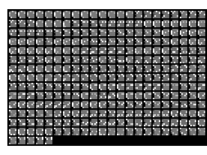
As shown in Fig. 6, VAE-ROC captures tangent space that is centered on the smooth manifold, which is modeled by the mean face . The rest of manifold deviated from the smooth manifold is captured by the principal direction vector . The larger the norm of is, the larger deviation from the smooth manifold can be captured. By regularizing the norm of , we can control how much proportion of manifold is captured by the smooth manifold. With cross validation, we find works best. Looking closely into the tangent space in the Fig. 6, each row shows faces on the tangent space of the mean face (red box at the center) that is deviated with the different weighted principal direction vectors (black box at the leftmost column).
We also confirm effectiveness of VAE-ROC quantitatively with the test log-likelihood of both models measured by Gaussian Parzen window as shown in Table. 1, where Rank Regularization (RR) is also applied to improve the quality of samples that VAE-ROC generates.
5.3 MNIST Dataset
| MNIST (10K) | |
|---|---|
| DBN [16] | |
| GAN [17] | |
| GMMN + AE [18] | |
| VAE-ROC | |
| VAE-DGF(5-500-300)[19] | |
| VAE-ROC(RR) | |
| Adv. AE [13] |
In this subsection, we learn VAE-ROC on real valued MNIST dataset [20] as shown in Fig. 7, where we only report the results of VAE-ROC because we failed to get the comparable result using Gaussian VAE with diagonal covariance matrix. Even with intensive hyper parameter search with random initial parameters, it is very hard to train the Gaussian VAE with diagonal covariance matrix on real valued MNIST dataset. However, by regularizing VAE-ROC with extreme weighted L1 regularization, VAE-ROC learns the manifold that Gaussian VAE was supposed to learn as shown in Fig. 7(b), where we are only to find noise in the tangent vector, which means its covariance matrix is closed to diagonal matrix.


To verify VAE-ROC quantitatively with existing models, we randomly divide the given 60,000 training set into 50,000 training set and 10,000 validation set in this experiment. We also scale the value into [0,1] to compare with other models. Moreover, we optimize our model with random hyper parameter search with 100 iterations and compare the test log-likelihood measured by Gaussian Parzen windows (fitted by 10,000 samples) where we find free parameter with validation set. We report the result in Table 2.


Qualitatively, we compare the generated samples and reconstructed images from VAE-ROC (RR) with the original images in Fig. 8. As shown Fig. 8(d), VAE-ROC (RR) successfully reconstructs the given data, which means MLP learns nonlinear basis for MNIST dataset. Based on these nonlinear basis, VAE-ROC (RR) generates digits with various style as shown in Fig. 8(a) with the corresponding principal direction vector in Fig. 8(b). Moreover, we verify the shape of latent code on validation dataset in Fig. 9. It shows isotropic contour, which enables VAE-ROC (RR) to generate quality samples than VAE-ROC.
5.4 UCI Auto Dataset
In the following two subsections, we compare GCVAE with VAE on two mixed variate datasets. In this subsection, we first visualize UCI Auto dataset with one hot encoding categorical variables and normalized continuous variables with zero mean and unit variance, which let us check whether the model is actually trained in SGD. UCI Auto dataset consists of 39211 1 Actually, it contains 398 instances, six instances of which have missing entry. We omit these instances with missing entry. Due to the lack of data, we use only 30 hidden units and 2 dimensional latent space and early stopping at 10,000 iterations of parameter updates. instances of automobiles, each of which has 8 dimensional values. Five of them are continuous variables and the rest of them are categorical variables (i.e. Country of origin, the number of cylinders and the model year). We randomly select 313 instances as a training set, 39 instances as validation set and the rest 40 instances as test set. We train GCVAE described in the subsection. 4 and the corresponding VAE (Gaussian and categorical outputs without copula) on UCI auto dataset.


As a generative model, GCVAE models data generating distribution on UCI Auto dataset, which can be evaluated by comparing the test log-likelihood on the distribution. Instead of using the exact value, we can approximate the distribution with samples from each model, which are used to fit kernel density estimator. In case there are only continuous variables, we may use Gaussian Parzen window method [21, 17]. However, we are treating a mixed variate dataset, which brings the following kernel density estimator for mixed variate dataset ( mixed with continuous and discrete variables ) [22]:
where is the number of samples to build kernel density estimator (10,000 samples), denotes a kernel function for categorical variable. It has in case and in otherwise. and are free parameters for kernel density estimator and selected via cross validation22
2
,
. . We describe how to sample from GCVAE in Appendix. B.
As shown in Table 3, we take randomly initiated 10 runs for each model and report mean and standard deviation, where we can find GCVAE shows better per-instance test log-likelihood than VAE measured by the kernel density estimator fit by samples from the corresponding model. We use no regularization in this experiment.
| UCI Auto (10K) | UCI SPECT (10K) | |
|---|---|---|
| VAE | ||
| GCVAE |
Qualitatively, we also check local dependency with Kendall’s tau as shown Fig. 11, where we first normalize covariance matrix of Gaussian copula and covert it by using the relationship between Kendall’s tau and Pearson correlation coefficient [23]. The number of cylinders and model year shows discordant pairs due to the 70’s oil crisis and horse power and weight shows concordance pair because more horse power needs bigger engine in general.
5.5 UCI SPECT Heart Dataset
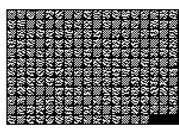


As shown in Fig. 12(a), UCI SPECT heart dataset describes medical diagnosis on cardiac disease with Single Proton Emission Computed Tomography (SPECT) images. Each instance consists of 22 binary predictors and binary predict that indicates normal and abnormal. We split the total 267 SPECT images into three subset: 213 instances for the training set and 27 instances for validation and test set respectively. After training, both models successfully capture the manifolds in Fig. 12(b) and Fig. 12(c). Both models adopt two 100 ReLU hidden units. GCVAE is not regularized by locality constraint. As the same manner as the previous subsection, we fit nonparametric kernel density estimator with the samples and report the mean and standard deviation of test log-likelihood in Table 3 with 10 runs of both models, which shows GCVAE models better than VAE quantitatively.
6 Conclusions
In this paper we have presented two extensions of the Gaussian VAE, leading to VAE-ROC and GCVAE. First, we have developed the VAE-ROC, where the local manifold structure in the unlabelled training dataset is approximated by a local principal direction at a position determined by the output of a neural network which takes the latent variable as input. The VAE-ROC was interpreted as an infinite mixture of probabilistic component analyzers, where mixture membership is smoothly varying, according to latent variables drawn from the standard multivariate Gaussian distribution. Second, we have developed the GCVAE to handle mixed categorical and continuous data, incorporating Gaussian copula to model local dependency in the mixed data. The technique known as ’continuous extension’ was used to take care of discrete variables together with continuous variables in the likelihood of mixed data. Experiments on various datasets demonstrated the useful behaviour of VAE-ROC and GCVAE, compared to the standard VAE.
Acknowledgments: This work was supported by Institute for Information & Communications Technology Promotion (IITP) grant funded by the Korea government (MSIP) [B0101-16-0307; Basic Software Research in Human-level Lifelong Machine Learning (Machine Learning Center)] and National Research Foundation (NRF) of Korea [NRF-2013R1A2A2A01067464].
References
- [1] D. P. Kingma and M. Welling. Auto-encoding variational Bayes. In Proceedings of the International Conference on Learning Representations (ICLR), Banff, Canada, 2014.
- [2] Y. Bengio, M. Monperrus, and H. Larochelle. Nonlocal estimation of manifold structure. Neural Computation, 18:2509–252, 2006.
- [3] R. B. Nelsen. An Introduction to Copulas. Springer, 2 edition, 2006.
- [4] B. S. Everitt. A finite mixture model for the clustering of mixed-mode data. Statistics & Probability Letters, 6(5):305–309, 1988.
- [5] P. D. Hoff. Extending the rank likelihood for semiparametric copula estimation. The Annals of Applied Statistics, 1(1):265–283, 2007.
- [6] M. Denuit and P. Lambert. Constraints on concordance measures in bivariate discrete data. Journal of Multivariate Analysis, 93:40–57, 2005.
- [7] L. Madsen and Y. Fang. Joint regression analysis for discrete longitudinal data. Biometrics, 67(3), 2011.
- [8] H. Liu, J. Lafferty, and L. Wasserman. The nonparanormal: Semiparametric estimation of high dimensional undirected graphs. Journal of Machine Learning Research, 10:2295–2328, 2009.
- [9] J. S. Murray, D. B. Dunson, L. Carin, and J. E. Lucas. Bayesian Gaussian copula factor models for mixed data. Journal of the American Statistical Association, 108(502):656–665, 2013.
- [10] M. Marbac, C. Biernacki, and V. Vandewalle. Model-based clustering of Gaussian copulas for mixed data, 2015. Preprint arXiv:1405.1299.
- [11] A. Sklar. Fonctions de répartition à n dimensions et leurs marges. Publ. Inst. Statist. Univ. Paris, 8:229–231, 1959.
- [12] B. Choroś, R. Ibragimov, and E. Permiakova. Copula estimation. In Copula Theory and Its Applications, pages 77–91. Springer, 2010.
- [13] A. Makhzani, J. Shlens, N. Jaitly, and I. Goodfellow. Adversarial autoencoders. In Proceedings of the International Conference on Learning Representations (ICLR), San Juan, Puerto Rico, 2016.
- [14] M. Magdon-Ismail and A. Atiya. Neural networks for density estimation. In Advances in Neural Information Processing Systems (NIPS), volume 11, 1999.
- [15] D. P. Kingma and J. L. Ba. ADAM: A method for stochastic optimization. In Proceedings of the International Conference on Learning Representations (ICLR), San Diego, CA, USA, 2015.
- [16] G. E. Hinton, S. Osindero, and Y. W. Teh. A fast learning algorithm for deep belief nets. Neural Computation, 18(7):1527–1554, 2006.
- [17] I. J. Goodfellow, J. Pouget-Abadie, M. Mirza, B. Xu, D. Warde-Farley, S. Ozair, A. Courville, and Y. Bengio. Generative adversarial nets. In Advances in Neural Information Processing Systems (NIPS), volume 27, 2014.
- [18] Y. Li, K. Swersky, and R. Zemel. Generative moment matching networks. In Proceedings of the International Conference on Machine Learning (ICML), Lille, France, 2015.
- [19] Z. Dai, A. Damianou, J. González, and N. Lawrence. Variational auto-encoded deep Gaussian processes. In Proceedings of the International Conference on Learning Representations (ICLR), San Juan, Puerto Rico, 2016.
- [20] Y. LeCun, L. Bottou, Y. Bengio, and P. Haffner. Gradient-based learning applied to document recognition. Proceedings of the IEEE, 86(11):2278–2324, 1998.
- [21] Y. Bengio, É. Thibodeau-Laufer, G. Alain, and J. Yosinski. Deep generative stochastic networks trainable by backprop. In Proceedings of the International Conference on Machine Learning (ICML), Beijing, China, 2014.
- [22] J. Aitchison and C. G. G. Aitken. Multivariate binary discrimination by the kernel method. Biometrika, 63(3):413–420, 1976.
- [23] C. Meyer. The bivariate normal copula. Communications in Statistics - Theory and Methods, 42(13):2402–2422, 2013.
Appendix A Gaussian Copula Density with
Proof.
In this section, we derive Gaussian copula with covariance matrix . Along with Sklar’s theorem, If , there exists unique copula function C: satisfying the following condition:
where is the CDF of univariate Gaussian distribution with zero mean and variance and denotes the CDF of multivariate normal distribution of zero mean vector and covariance matrix that has as th entry of diagonal entries. Inversion of Sklar’s theorem, we have:
| (19) | |||||
where and is the CDF of univariate standard normal distribution and denotes normal score. The second line stands because . By differentiating Eq. 19 with respect , we have Gaussian copula density as follows:
∎
Appendix B Sampling from Gaussian copula
In this subsection, we briefly review how to sample from Gaussian copula. Let us assume and we have Gaussian copula having as covariance matrix. Then, we have:
By analyzing samples from various cases of parameters , we can more clearly understand how GCVAE models local dependency across input dimensions. Fig. 13 shows that characteristics of samples with such in bivariate Gaussian copula. As shown in Fig. 13(a), If the signs of and are the same, two dimensions have concordant pairs and if they are opposite, two dimensions have discordant pairs. If they are all zeros, there is no dependency between two dimensions. As shown in Fig. 13(b), non-decreasing transformation of any dimension in doesn’t change the copula density. Fig. 13(c) shows how noise parameter affects copula density function. The large the , the lesser dependency two dimensions have. Finally, 13(d) shows how norm of principal vector affect the copula density function. The larger the norm is, the more stringent to the noise.


samples on unit rectangle.