跳到论文正文
W Papers独立论文阅读器 arXiv:1604.04930 论文正文 计算阅读时间 · 0%
引用这篇论文根据当前论文元数据生成,正式投稿前建议核对。


License: arXiv.org perpetual non-exclusive license
arXiv:1604.04930v2 [math.AP] 10 Nov 2016

Asymptotic Analysis of the Ginzburg-Landau Functional on Point Clouds

Matthew Thorpe Affiliation: Carnegie Mellon University, Pittsburgh, PA 15213, USA    Florian Theil Affiliation: University of Warwick, Coventry, CV4 7AL, UK
November 2016
Abstract

The Ginzburg-Landau functional is a phase transition model which is suitable for classification type problems. We study the asymptotics of a sequence of Ginzburg-Landau functionals with anisotropic interaction potentials on point clouds Ψn\Psi_{n} where nn denotes the number data points. In particular we show the limiting problem, in the sense of Γ\Gamma-convergence, is related to the total variation norm restricted to functions taking binary values; which can be understood as a surface energy. We generalize the result known for isotropic interaction potentials to the anisotropic case and add a result concerning the rate of convergence.

1 Introduction

1.1 Finite Dimensional Modeling

In the age of ‘big data’ the mathematical modeller is often without a physical model and instead uses a data driven approach for which graphical models are a powerful tool. Graphical based modelling techniques are used across a very broad spectrum of problems from social science type problems, such as identifying communities [39, 18, 44, 46, 22], to image segmentation [29, 6], to cell biology [14], to modelling the world wide web [7, 14, 12, 21] and many more. Anisotropic models, studied in this paper, have found applications in cosmological models [28, 34], modelling outbreaks of disease [33] and image recognition [47].

Graphical models are based upon pairwise similarities which practitioners can design based on expert knowledge. The measure of similarity (on pairs) then defines a geometry (on a data set). The motivation in this paper is to consider a graphical approach to the classification problems. Given a measure of similarity we wish to define a labelling using the geometry of the graph.

The problem is given data Ψn={ξi}i=1n⊂X\Psi_{n}=\{\xi_{i}\}_{i=1}^{n}\subset X, where X⊂ℝdX\subset\mathbb{R}^{d}, find μ:Ψn→ℝ\mu:\Psi_{n}\to\mathbb{R} that labels each data point. The labelling is constructed so that μ⁡(ξi)=0\mu(\xi_{i})=0 means that ξi\xi_{i} is associated with the class 0 and μ⁡(ξi)=1\mu(\xi_{i})=1 means that ξi\xi_{i} is associated with the class 1. For a finite number of observations we allow a soft classification however the scaling is chosen such that in the data rich limit classifiers are binary valued. The motivation for our approach is to validate approximating the hard classification problem by a soft classification problem. The soft classification problem is in general numerically easier [24] and therefore more appealing to the practitioner. However one also wants to be precise in regards to which class a data point belongs. Minimizers of the Ginzburg-Landau functional are used as a classification tool [42] in order to allow for phase transitions which allow a soft classification approach whilst also penalizing states that are not close to a hard classification.

Another important application for this work is in designing classifiers. By not assuming that the model is isotropic we allow greater flexibility which allows one to choose some features as more important than others. The next subsection contains a simple example which shows how the design choice can affect the classification.

Assessing the validity of such an approach is of high importance. This is especially true as there is no natural link between the data generating process and the choice of classifier. In particular we argue that although using the Ginzburg-Landau functional is a good choice due to its phase transition properties it is by no means the only available option. When one can make a connection between classifier and data generating process, e.g. maximum likelihood estimators, then this link motivates the methodology. Without such connection one needs to do more, such as show the estimators have desirable properties, in order to justify the approach. Other approaches that use classifiers that are detached from the data generating process include [41] where the authors prove the convergence of the kk-means method using similar variational techniques.

An important criterion for validating the model is the behaviour in the large data limit. When increasing the size of the data set one should expect to see stability in classifiers. In particular this requires convergence in the large data limit and the existence of a limiting (data rich) model. When one has a data generating model, i.e. there is some truth, then one can talk about consistency. In the situation considered in this paper there is no truth so instead we use solutions to the limiting model. Knowledge of the limiting model gives an insight into what features one should expect for estimates from the finite data problem. In particular this paper considers three questions:

  1. (P1)

    Do estimated classifiers μn\mu_{n} converge as n→∞n\to\infty?

  2. (P2)

    Can we attach some meaning to any limit of μn\mu_{n}? I.e. does there exists a limiting problem?

  3. (P3)

    Can we characterize the rate of convergence of estimators?

The primary results of this paper concern the first two questions. It is shown that estimates μn\mu_{n} converge to the solution of a limiting problem. Furthermore solutions to the limiting problem are binary valued which means we expect estimates μn\mu_{n} for large nn to be approximately hard classifiers. For the third question we give some preliminary results into characterizing the rate in a simplified example. We believe these results will hold under more generality than stated here and it is the objective of ongoing work to extend them.
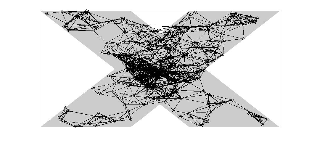
Refer to caption
Figure 1: An example graph. For the classifier estimates see Figure 2.

Our approach is motivated by [1, 25, 42]. Classifiers are constructed as the solution of a variational problem which is common in statistical problems, e.g. maximum likelihood and maximum-a-posterior problems. In particular minimizers of the Ginzburg-Landau functional, a phase transition model popular in material science and image segmentation, are used as classifiers. In the context of the 2-class classification problem the two phases are the classes and the phase transition corresponds to the set {x∈Ψn:μn​(x)∈(c,1−c)}\left\{x\in\Psi_{n}\,:\,\mu_{n}(x)\in(c,1-c)\right\} for some c∈(0,1)c\in(0,1), e.g. c=0.1c=0.1. This is the subset of Ψn\Psi_{n} that are not strongly associated with either class.

Classifiers μn:Ψn→ℝ\mu_{n}:\Psi_{n}\to\mathbb{R} are constructed as follows. Let V:ℝ→[0,∞)V:\mathbb{R}\to[0,\infty) be a potential such that states taking the value 0 or 1 is favoured. For example V⁡(t)=t2​(t−1)2V(t)=t^{2}(t-1)^{2}. A graph is constructed by taking the vertices as the set Ψn={ξi}i=1n⊂ℝd\Psi_{n}=\{\xi_{i}\}_{i=1}^{n}\subset\mathbb{R}^{d} and weighting edges

Wi​j=ηϵ​(ξi−ξj):=1ϵd​φ∘π⁡(ξi−ξjϵ)W_{ij}=\eta_{\epsilon}(\xi_{i}-\xi_{j}):=\frac{1}{\epsilon^{d}}\varphi\circ\pi\left(\frac{\xi_{i}-\xi_{j}}{\epsilon}\right) (1)

where π:X→ℝ\pi:X\to\mathbb{R} is a given one-dimensional map so that π⁡(ξi)\pi(\xi_{i}) represents a feature of ξi\xi_{i} and φ:ℝ→[0,∞)\varphi:\mathbb{R}\to[0,\infty) penalizes the difference π⁡(ξi−ξj)\pi(\xi_{i}-\xi_{j}). We say that there is an edge between ξi\xi_{i} and ξj\xi_{j} if Wi​j>0W_{ij}>0, for example see Figure 1. For a function μn\mu_{n} on Ψn\Psi_{n} the graph energy ℰn​(μn)∈[0,∞]\mathcal{E}_{n}(\mu_{n})\in[0,\infty] is defined by

ℰn​(μn)=1ϵn​1n​∑i=1nV⁡(μn​(ξi))+1ϵn​1n2​∑i,jWi​j​|μn​(ξi)−μn​(ξj)|.\mathcal{E}_{n}(\mu_{n})=\frac{1}{\epsilon_{n}}\frac{1}{n}\sum_{i=1}^{n}V(\mu_{n}(\xi_{i}))+\frac{1}{\epsilon_{n}}\frac{1}{n^{2}}\sum_{i,j}W_{ij}|\mu_{n}(\xi_{i})-\mu_{n}(\xi_{j})|. (2)

Our classifier is given as the minimizer of ℰn\mathcal{E}_{n}.

We call the map π:X→ℝ\pi:X\to\mathbb{R} the feature projection as it allows the practitioner to include feature selection of the data ξi\xi_{i}. For example one may decide that two data points should be considered similar based on the pairwise difference. In this case an appropriate choice would be the weighted Euclidean distance π⁡(x)=∑i=1dwi​|xi|2\pi(x)=\sqrt{\sum_{i=1}^{d}w_{i}|x_{i}|^{2}}. The isotropic case would correspond to weights wi=1w_{i}=1. Other choices could be to include correlations between dimensions, for example π⁡(x)=∑i,j=1dwi​j​|xi|​|xj|\pi(x)=\sqrt{\sum_{i,j=1}^{d}w_{ij}|x_{i}||x_{j}|}.

The authors of [25] study the asymptotic properties of the graph total variation defined by

G​T​Vn​(μn):=1ϵn​1n2​∑i,jWi​j​|μn​(ξi)−μn​(ξj)|GTV_{n}(\mu_{n}):=\frac{1}{\epsilon_{n}}\frac{1}{n^{2}}\sum_{i,j}W_{ij}|\mu_{n}(\xi_{i})-\mu_{n}(\xi_{j})| (3)

when Wi​jW_{ij} is isotropic, i.e. π⁡(x)=|x|\pi(x)=|x|. In the special case that μn​(ξi)∈{0,1}\mu_{n}(\xi_{i})\in\{0,1\} this reduces to the graph cut of Ψn\Psi_{n}, i.e. if (μn)−1​(0)=A0(\mu_{n})^{-1}(0)=A_{0} and (μn)−1​(1)=A1(\mu_{n})^{-1}(1)=A_{1} then

G​T​Vn​(μn)=1ϵn​1n2​∑ξi∈A0∑ξj∈A1Wi​j.GTV_{n}(\mu_{n})=\frac{1}{\epsilon_{n}}\frac{1}{n^{2}}\sum_{\xi_{i}\in A_{0}}\sum_{\xi_{j}\in A_{1}}W_{ij}.

In particular the authors in [25] show the Γ\Gamma-convergence of G​T​VnGTV_{n} to a weighted total variation T​V​(⋅,ρ,η)TV(\cdot;\rho,\eta) given by

TV(μ;ρ,η):=σηsup{∫Xμdiv(ϕ)dx:|ϕ(x)|≤ρ2(x)∀x∈X,ϕ∈Cc∞(X;ℝd)},TV(\mu;\rho,\eta):=\sigma_{\eta}\sup\left\{\int_{X}\mu\mathrm{div}(\phi)\,\mathrm{d}x\,:\,|\phi(x)|\leq\rho^{2}(x)\,\forall x\in X,\phi\in C_{c}^{\infty}(X;\mathbb{R}^{d})\right\},

and L1L^{1}-compactness for any sequence μn\mu_{n} with supn(G​T​Vn​(μn)+‖μn‖L1)<∞\sup_{n}(GTV_{n}(\mu_{n})+\|\mu_{n}\|_{L^{1}})<\infty.

We wish to allow for soft classification and the total variation term alone is not enough to be able to do this informatively. The classification approach is made more robust by including a first order term V:ℝ→[0,∞)V:\mathbb{R}\to[0,\infty) which penalizes associating a data point to more than one class. See, for example, Figure 2 for a comparison. It is not trivial that the convergence results in [25] will survive adding a penalty term.

Refer to caption
Refer to caption
Refer to caption
Refer to caption
Figure 2: The top row shows the minimizers of ℰn\mathcal{E}_{n} and the bottom row shows the minimizers of G​T​VnGTV_{n} for the graph given in Figure 1 conditioned on the node closest to each corner taking either 0 or 1. The left column is conditioned to have 0 in the bottom corners and 1 in the top corners. The right column has 0 in the bottom left and top right corners and 1 in the top left and bottom right corners. There is very little difference between the outputs on the left but on the right the G​T​VnGTV_{n} term fails to pick out the singularity at the center.

Finding minimizers of ℰn\mathcal{E}_{n} is also an important problem but is not addressed in this paper. We instead refer to [9, 10] for numerical methods.

1.2 Example: Classification Dependence on the Choice of η\eta

Through a toy problem we demonstrate how the interaction potential can be used to pick out features of the practitioners choice. Data are points ξi=(ξ1​i,ξ2​i)∈ℝ2\xi_{i}=(\xi_{1i},\xi_{2i})\in\mathbb{R}^{2} generated from four classes. For a fixed α\alpha the feature projection π:ℝ2→[0,∞)\pi:\mathbb{R}^{2}\to[0,\infty) is defined by the weighted Euclidean norm

π⁡(ξ)=(1−α)​ξ12+α​ξ22.\pi(\xi)=\sqrt{(1-\alpha)\xi_{1}^{2}+\alpha\xi_{2}^{2}}.

For α≈1\alpha\approx 1 the classifiers are dominated by differences in the first coordinate whilst for α≈0\alpha\approx 0 the classifiers are dominated by differences in the second coordinate. More precisely, let

μ1​(ξi)\displaystyle\mu_{1}(\xi_{i}) ={1if ​ξ2​i≤c10otherwise\displaystyle=\left\{\begin{array}[]{ll}1&\text{if }\xi_{2i}\leq c_{1}\\ 0&\text{otherwise}\end{array}\right.
μ2​(ξi)\displaystyle\mu_{2}(\xi_{i}) ={1if ​ξ1​i≤c20otherwise.\displaystyle=\left\{\begin{array}[]{ll}1&\text{if }\xi_{1i}\leq c_{2}\\ 0&\text{otherwise.}\end{array}\right.

Then define

Δ​ℰn=ℰn​(μ1)−ℰn​(μ2).\Delta\mathcal{E}_{n}=\mathcal{E}_{n}(\mu_{1})-\mathcal{E}_{n}(\mu_{2}).

The results are given in Figure 3.

55101015152020252515152020252530303535ξ1​i\xi_{1i}ξ2​i\xi_{2i}
000.20.20.40.40.60.60.80.811−2-20022⋅10−2\cdot 10^{-2}α\alphaΔ​ℰn\Delta\mathcal{E}_{n}
Figure 3: The figure on the left shows a realisation of the data. The interactions are parameterized by a potential α\alpha which favours horizontal partitions for α≈0\alpha\approx 0 and vertical partitions for α≈1\alpha\approx 1 as shown by the figure on the right.

1.3 The Limiting Model

Rather surprisingly the problem of soft classifications for finite data sets and hard classification in the limit has received relatively little attention in the literature. However it is well known that for finite data one can recover the kk-means algorithm (hard classification) from the expectation-maximization algorithm (soft classification) in the zero-variance limit for the Gaussian mixture model and the Dirichlet process mixture model [31, 35].

The results of this paper concern the asymptotics of the minimum and minimizers of ℰn\mathcal{E}_{n}, where ϵn→0\epsilon_{n}\to 0 as n→∞n\to\infty. The advantages of scaling ϵn\epsilon_{n} to zero are two-fold. The first is that the matrix W=(Wi​j)i​jW=(W_{ij})_{ij} is sparse and therefore we expect the minimization to be numerically less expensive than solving the minimization with a non-sparse matrix (since the sparse minimization has O⁡(n)O(n) terms and the non-sparse minimization O⁡(n2)O(n^{2}) terms). The second is to improve resolution of the boundary. One can think of soft classification as estimating the probability that a data point belongs to a certain class and the hard classification problem as estimating the boundaries where one class is more likely than all others. By scaling ϵn→0\epsilon_{n}\to 0 it will be shown that the limiting minimization problem is a hard classification. For example, Figure 4 shows (for a fixed number of data points) improved resolution in the boundary between classes as ϵ→0\epsilon\to 0. See also [24].

Assume X⊂ℝdX\subset\mathbb{R}^{d} and define ℰ∞:L1​(X)→[0,∞]\mathcal{E}_{\infty}:L^{1}(X)\to[0,\infty] by

ℰ∞​(μ)={∫∂{μ=1}σ(n(x))ρ2(x)dℋd−1(x)if ​μ∈L1​(X,{0,1})∞otherwise\mathcal{E}_{\infty}(\mu)=\left\{\begin{array}[]{ll}\int_{\partial\{\mu=1\}}\sigma(n(x))\rho^{2}(x)\;\mathrm{d}\mathcal{H}^{d-1}(x)&\text{if }\mu\in L^{1}(X;\{0,1\})\\ \infty&\text{otherwise}\end{array}\right. (4)

where n⁡(x)n(x) is the outward unit normal for the set ∂{μ=1}\partial\{\mu=1\}, ℋd−1\mathcal{H}^{d-1} is the d−1d-1 dimensional Hausdorff measure and

σ⁡(ν)=∫ℝdφ⁡(π⁡(x))​|x⋅ν|​𝑑x.\sigma(\nu)=\int_{\mathbb{R}^{d}}\varphi(\pi(x))|x\cdot\nu|\;\mathrm{d}x.

It will be shown, in the sense of Γ\Gamma-convergence, that ℰ∞\mathcal{E}_{\infty} is the limiting problem and any sequence such that ℰn​(μn)\mathcal{E}_{n}(\mu_{n}) is bounded is precompact in an appropriate topology. In particular this allows one to apply the results of this paper to infer the consistency of the constrained minimization problem (see Section 2.2).

Figure 4: Both figures were classified using the Ginzburg-Landau functional. The one on the left used a larger ϵ\epsilon than the one on the right. The figure shows that the smaller value of ϵ\epsilon gives a much better resolution in the boundary.

We now briefly discuss the convergence of μn→μ\mu_{n}\to\mu. Since each μn\mu_{n} is defined on a different space (the domain of each μn\mu_{n} is Ψn\Psi_{n}) it is not straightforward what is meant by convergence of μn→μ∞\mu_{n}\to\mu_{\infty}. By defining a map Tn:X→ΨnT_{n}:X\to\Psi_{n} one can compare μn\mu_{n} to μ∞\mu_{\infty} by defining the piecewise constant approximation of μn\mu_{n}. Formally we can say μn→μ∞\mu_{n}\to\mu_{\infty} in T​L1TL^{1} if μn∘Tn→μ∞\mu_{n}\circ T_{n}\to\mu_{\infty} in L1L^{1}, this is discussed further in Section 3.4.

We also include preliminary results towards characterizing the rate of convergence by considering a simple example when μ=𝕀E\mu=\mathbb{I}_{E} for a polyhedral set E⊂XE\subset X and looking at the convergence in mean square:

𝔼​|ℰn​(μ)−ℰ∞​(μ)|2=𝔼​|G​T​Vn​(μ)−T​V​(μ,ρ,η)|2.\mathbb{E}\left|\mathcal{E}_{n}(\mu)-\mathcal{E}_{\infty}(\mu)\right|^{2}=\mathbb{E}\left|GTV_{n}(\mu)-TV(\mu;\rho,\eta)\right|^{2}.

We give an expansion of the above in terms of ϵn\epsilon_{n} and nn. A further overview of these results is given in Section 2.3 and the proofs in Section 6.

The outline of the paper is as follows. In Section 2 the main result, Theorem 2.3 (the convergence of the unconstrained minimization problem), is given. We also include an overview of the preliminary rate of convergence results to be found in Section 6. Section 3 contains the background material and in particular: notation, a brief overview on Γ\Gamma-convergence, background on total variation distances and the key details required from transportation theory. In Section 4 the proof of the first part of Theorem 2.3 (the compactness result) is given. And in Section 5 the proof is completed with the Γ\Gamma-convergence result. Finally in Section 6 we make the preliminary calculation regarding the rate of convergence of “ℰn→ℰ∞\mathcal{E}_{n}\to\mathcal{E}_{\infty}”.

2 Statement of Main Result and Assumptions

The assumptions on V,φV,\varphi and π\pi are given in the following definition.

Definition 2.1.

We say that the functions (ρ,ϵn,V,φ,π)(\rho,\epsilon_{n},V,\varphi,\pi) where ρ:ℝn→[0,∞)\rho:\mathbb{R}^{n}\to[0,\infty), V:ℝ→[0,∞)V:\mathbb{R}\to[0,\infty), φ:ℝ→[0,∞)\varphi:\mathbb{R}\to[0,\infty) and π:ℝd→ℝ\pi:\mathbb{R}^{d}\to\mathbb{R} are ℰn\mathcal{E}_{n}-admissible if the following conditions hold.

  1. 1.

    The support of ρ\rho is XX where X⊂ℝdX\subset\mathbb{R}^{d} is open, bounded, connected, Lipschitz boundary and 1≤d<∞1\leq d<\infty.

  2. 2.

    On XX we have that ρ\rho is a continuous probability density (∫Xρ⁡(x)​𝑑x=1\int_{X}\rho(x)\,\mathrm{d}x=1) and bounded above and below by positive constants, i.e.

    0<infx∈Xρ⁡(x)≤supx∈Xρ⁡(x)<∞.0<\inf_{x\in X}\rho(x)\leq\sup_{x\in X}\rho(x)<\infty.
  3. 3.

    ϵn−1=o⁡(fd​(n))\epsilon_{n}^{-1}=o(f_{d}(n)) where

    fd​(n)={nlog⁡log⁡nif ​d=1n(log⁡n)32if ​d=2nlog⁡ndif ​d≥3.f_{d}(n)=\left\{\begin{array}[]{ll}\sqrt{\frac{n}{\log\log n}}&\text{if }d=1\\ \frac{\sqrt{n}}{(\log n)^{\frac{3}{2}}}&\text{if }d=2\\ \sqrt[d]{\frac{n}{\log n}}&\text{if }d\geq 3.\end{array}\right.
  4. 4.

    The support of η=φ∘π\eta=\varphi\circ\pi is compact.

  5. 5.

    η⁡(0)>0\eta(0)>0.

  6. 6.

    For all δ>0\delta>0 there exists cδ,αδ>0c_{\delta},\alpha_{\delta}>0 such that if |x−y|<δ|x-y|<\delta then η⁡(y)≥cδ​η​(αδ​x)\eta(y)\geq c_{\delta}\eta(\alpha_{\delta}x) and furthermore cδ,αδ→1c_{\delta},\alpha_{\delta}\to 1 as δ→0\delta\to 0.

  7. 7.

    V⁡(y)=0V(y)=0 if and only if y∈{0,1}y\in\{0,1\}.

  8. 8.

    VV is continuous.

  9. 9.

    There exists r>0r>0 and τ>0\tau>0 such that if |t|≥r|t|\geq r then V⁡(t)≥τ​|t|V(t)\geq\tau|t|.

The lower bound on ϵn\epsilon_{n} implies the graph with vertices Ψn\Psi_{n} and edges weighted by Wi​jW_{ij} is (with probability one) eventually connected [38, Theorem 13.2].

Note that a consequence of 4 and 6 is that σ⁡(ν)<∞\sigma(\nu)<\infty however 4 also excludes any π\pi that is linear. For example if π⁡(x)=w⋅x\pi(x)=w\cdot x then there exists w′w^{\prime} orthogonal to ww such that w⋅w′=0w\cdot w^{\prime}=0 (for d≥2d\geq 2). Then π⁡(α​w′)=0\pi(\alpha w^{\prime})=0 for all α\alpha and in particular η⁡(α​w′)=η⁡(0)>0\eta(\alpha w^{\prime})=\eta(0)>0. Therefore the support of η\eta is not compact. We discuss the linear case more in the following subsection.

Condition 6 gives the required scaling in φ∘π\varphi\circ\pi. If Tn:X→ΨnT_{n}:X\to\Psi_{n} is a map such that Tn​#​P=PnT_{n\#}P=P_{n} then the continuous approximation of the weights Wi​jW_{ij} reads as

Wi​j=1ϵnd​φ∘π⁡(ξi−ξjϵn)≈1ϵnd​∫Tn−1​(ξi)∫Tn−1​(ξj)φ∘π⁡(x−yϵn)​𝑑x​𝑑y.W_{ij}=\frac{1}{\epsilon_{n}^{d}}\varphi\circ\pi\left(\frac{\xi_{i}-\xi_{j}}{\epsilon_{n}}\right)\approx\frac{1}{\epsilon_{n}^{d}}\int_{T_{n}^{-1}(\xi_{i})}\int_{T_{n}^{-1}(\xi_{j})}\varphi\circ\pi\left(\frac{x-y}{\epsilon_{n}}\right)\;\mathrm{d}x\;\mathrm{d}y.

Condition 6 is sufficient to formalise this reasoning. We give two different classes of functions in Proposition 2.2 below that satisfy the assumptions. The first is a subset of isotropic functions that we extend in Corollary 2.4, the second is a set of indicator functions.

Proposition 2.2.

Assume that either

  1. 1.

    φ:[0,∞)→[0,∞)\varphi:[0,\infty)\to[0,\infty) is decreasing, φ⁡(0)>0\varphi(0)>0, is Lipschitz with compact support and π:ℝd→[0,∞)\pi:\mathbb{R}^{d}\to[0,\infty) is defined by π⁡(x)=|x|\pi(x)=|x|, or

  2. 2.

    φ⁡(0)>0\varphi(0)>0, φ⁡(1)=0\varphi(1)=0, π:ℝd→{0,1}\pi:\mathbb{R}^{d}\to\{0,1\} is given by π​(x)=𝕀Ec​(x)\pi(x)=\mathbb{I}_{E^{c}}(x) for an open, bounded and convex set E⊂ℝdE\subset\mathbb{R}^{d} with 0∈E0\in E.

Then (φ,π)(\varphi,\pi) are ℰn\mathcal{E}_{n}-admissible.

We prove the above proposition in Appendix A. We now state the main result. The key idea is that optimal transportation theory provides a natural extension of μn:Ψn→ℝ\mu_{n}:\Psi_{n}\to\mathbb{R} to μ~n:X→ℝ\tilde{\mu}_{n}:X\to\mathbb{R} for which we can use to define the convergence μn→μ\mu_{n}\to\mu. This is formalised as convergence in T​L1TL^{1}, see Section 3.4. Establishing Γ\Gamma-convergence of functionals, see Definition 3.1, and the compactness of minimizers leads to the convergence of minimizers as in Theorem 3.2. We use the notation L1​(Ψn)L^{1}(\Psi_{n}) as convenient notation for functions defined on Ψn\Psi_{n}. We define the space B⁡(X,ρ,η)B(X;\rho,\eta), the space of functions of bounded variation with respect to a measure ρ\rho and a interaction potential η\eta, in Definition 3.3.

Theorem 2.3.

Let ℰn:L1​(Ψn)→[0,∞)\mathcal{E}_{n}:L^{1}(\Psi_{n})\to[0,\infty) and ℰ∞:L1​(X)→[0,∞]\mathcal{E}_{\infty}:L^{1}(X)\to[0,\infty] be defined by (2) and (4) respectively. If (ρ,ϵn,V,φ,π)(\rho,\epsilon_{n},V,\varphi,\pi) are ℰn\mathcal{E}_{n}-admissible (in the sense of Definition 2.1) and ξi∼iidρ\xi_{i}\stackrel{{\scriptstyle\mathrm{iid}}}{{\sim}}\rho then, with probability one, the following hold

  1. 1.

    Compactness: Let μn\mu_{n} be a sequence of functions on Ψn\Psi_{n} such that supn∈ℕℰn​(μn)<∞\sup_{n\in\mathbb{N}}\mathcal{E}_{n}(\mu_{n})<\infty then μn\mu_{n} is relatively compact in T​L1TL^{1} and each cluster point is in B​V​(X,ρ,φ∘π)∩L1​(X,{0,1})BV(X;\rho,\varphi\circ\pi)\cap L^{1}(X;\{0,1\}).

  2. 2.

    Γ\Gamma-limit: We have

    Γ-limn→∞⁡ℰn=ℰ∞.\Glim_{n\to\infty}\mathcal{E}_{n}=\mathcal{E}_{\infty}.

The compactness result is proved in Section 4 and the Γ\Gamma-convergence result in Section 5.

Proposition 2.2 allows one to apply Theorem 2.3 to isotropic weights Wi​jW_{ij} when φ\varphi is decreasing, φ⁡(0)>0\varphi(0)>0 and Lipschitz. We now show that the Lipschitz assumption can be removed.

Corollary 2.4.

Let ℰn:L1​(Ψn)→[0,∞)\mathcal{E}_{n}:L^{1}(\Psi_{n})\to[0,\infty) and ℰ∞:L1​(X)→[0,∞]\mathcal{E}_{\infty}:L^{1}(X)\to[0,\infty] be defined by (2) and (4) respectively. If

  1. ∙\bullet

    ρ\rho satisfies conditions 1-3 in Definition 2.1,

  2. ∙\bullet

    ξi∼iidρ\xi_{i}\stackrel{{\scriptstyle\mathrm{iid}}}{{\sim}}\rho,

  3. ∙\bullet

    φ:[0,∞)→[0,∞)\varphi:[0,\infty)\to[0,\infty) is decreasing, compactly supported, φ⁡(0)>0\varphi(0)>0 and continuous at 0,

  4. ∙\bullet

    π⁡(x)=|x|\pi(x)=|x|, and

  5. ∙\bullet

    VV satisfies conditions 11-13 in Definition 2.1

then, with probability one, the conclusions of Theorem 2.3 hold.

We prove the corollary in Appendix B

2.1 Convergence of the Ginzburg-Landau Functional for Linear Feature Projections

After Definition 2.1 we discussed how the compact support assumption on η=φ∘π\eta=\varphi\circ\pi did not allow for linear π\pi. One case that is of interest, that is not covered by Theorem 2.3 or Corollary 2.4 is π⁡(x)=xi\pi(x)=x_{i} that corresponds to weighting the graph based on differences in one direction only.

This case is of particular interest for high dimensional data. If the data comes from a high, potentially infinite, dimensional space then it becomes necessary to identify a finite number of principal dimensions upon which to define the edge weights. Isotropic weights are unrealistic in high dimensions and infeasible in infinite dimensions due to the lack of integrability of η\eta. This motivates our study of linear π\pi, which can include π⁡(x)=∑i∈𝒦xi\pi(x)=\sum_{i\in\mathcal{K}}x_{i} for a finite set 𝒦\mathcal{K}. Although we do not consider infinite dimensional data spaces here we believe the results of this section can be extended from the finite dimensional setting, albeit with a modified limit ℰ^∞\hat{\mathcal{E}}_{\infty} to the one we define in (6). With a more thorough treatment one should also be able to extend the convergence results of this subsection (i.e. to infinite dimensional spaces) to non-linear π\pi.

The underlying problem, and why we should not expect a linear choice of π\pi to imply that ℰ∞\mathcal{E}_{\infty} is well defined, is that it becomes harder to ensure that σ⁡(ν)<∞\sigma(\nu)<\infty. In particular, we expect ℰ∞≡+∞\mathcal{E}_{\infty}\equiv+\infty. In many applications we anticipate that only a small number of dimensions are relevant and hence we, in this section, consider the classifier as a functional on a projected data space. We define Ψ^n={ξ^i}i=1n⊂ℝ\hat{\Psi}_{n}=\{\hat{\xi}_{i}\}_{i=1}^{n}\subset\mathbb{R} by ξ^i=π⁡(ξi)\hat{\xi}_{i}=\pi(\xi_{i}) and μ^n:Ψ^n→[0,∞)\hat{\mu}_{n}:\hat{\Psi}_{n}\to[0,\infty). We now consider the energy

ℰ^n​(μ^n)=1ϵn​1n​∑i=1nV⁡(μ^n​(ξ^i))+1ϵn​1n2​∑i,jW^i​j​|μ^n​(ξ^i)−μ^n​(ξ^j)|\hat{\mathcal{E}}_{n}(\hat{\mu}_{n})=\frac{1}{\epsilon_{n}}\frac{1}{n}\sum_{i=1}^{n}V(\hat{\mu}_{n}(\hat{\xi}_{i}))+\frac{1}{\epsilon_{n}}\frac{1}{n^{2}}\sum_{i,j}\hat{W}_{ij}|\hat{\mu}_{n}(\hat{\xi}_{i})-\hat{\mu}_{n}(\hat{\xi}_{j})| (5)

where

W^i​j=1ϵn​φ∘π⁡(ξi−ξjϵn)=1ϵn​φ​(ξ^i−ξ^jϵn).\hat{W}_{ij}=\frac{1}{\epsilon_{n}}\varphi\circ\pi\left(\frac{\xi_{i}-\xi_{j}}{\epsilon_{n}}\right)=\frac{1}{\epsilon_{n}}\varphi\left(\frac{\hat{\xi}_{i}-\hat{\xi}_{j}}{\epsilon_{n}}\right).

We point out that the scaling is with respect to ϵn\epsilon_{n} rather than ϵnd\epsilon_{n}^{d} as in (1). In this case the Γ\Gamma-limit ℰ^∞:L1​(ℝ)→[0,∞]\hat{\mathcal{E}}_{\infty}:L^{1}(\mathbb{R})\to\mathbb{[}0,\infty] is given by

ℰ^∞(μ^)=σ^∑x∈∂{μ^=1}(∫π−1​(x)ρ(y)dy)2\hat{\mathcal{E}}_{\infty}(\hat{\mu})=\hat{\sigma}\sum_{x\in\partial\{\hat{\mu}=1\}}\left(\int_{\pi^{-1}(x)}\rho(y)\;\mathrm{d}y\right)^{2} (6)

where

σ^=∫ℝφ⁡(x)​|x|​𝑑x.\hat{\sigma}=\int_{\mathbb{R}}\varphi(x)|x|\;\mathrm{d}x.

The analogous assumptions are given in the definition below.

Definition 2.5.

We say that the functions (ρ,ϵn,V,φ,π)(\rho,\epsilon_{n},V,\varphi,\pi) where ρ:ℝd→[0,∞)\rho:\mathbb{R}^{d}\to[0,\infty), V:ℝ→[0,∞)V:\mathbb{R}\to[0,\infty), φ:ℝ→[0,∞)\varphi:\mathbb{R}\to[0,\infty) and π:ℝd→ℝ\pi:\mathbb{R}^{d}\to\mathbb{R} are ℰ^n\hat{\mathcal{E}}_{n}-admissible if the following hold.

  1. 1.

    The support of ρ\rho is XX where X⊂ℝdX\subset\mathbb{R}^{d} and the support of π#​ρ\pi_{\#}\rho is open, bounded and connected.

  2. 2.

    On XX we have that ρ\rho is a continuous probability density, bounded above and infx∈Xπ#​ρ​(x)>0\inf_{x\in X}\pi_{\#}\rho(x)>0.

  3. 3.

    ϵn−1=o⁡(f1​(n))\epsilon_{n}^{-1}=o(f_{1}(n)) where f1f_{1} is given in Definition 2.1.

  4. 4.

    π\pi is linear.

  5. 5.

    The support of φ\varphi is compact.

  6. 6.

    φ⁡(0)>0\varphi(0)>0.

  7. 7.

    For all δ>0\delta>0 there exists cδ,αδ>0c_{\delta},\alpha_{\delta}>0 such that if |x−y|<δ|x-y|<\delta then φ⁡(y)≥cδ​φ​(αδ​x)\varphi(y)\geq c_{\delta}\varphi(\alpha_{\delta}x) and furthermore cδ,αδ→1c_{\delta},\alpha_{\delta}\to 1 as δ→0\delta\to 0.

  8. 8.

    V⁡(y)=0V(y)=0 if and only if y∈{0,1}y\in\{0,1\}.

  9. 9.

    VV is continuous.

  10. 10.

    There exists r>0r>0 and τ>0\tau>0 such that if |t|≥r|t|\geq r then V⁡(t)≥τ​|t|V(t)\geq\tau|t|.

The convergence theorem is given below.

Theorem 2.6.

Let Ψ^n={ξ^i}i=1n\hat{\Psi}_{n}=\{\hat{\xi}_{i}\}_{i=1}^{n} where ξ^i=π⁡(ξi)\hat{\xi}_{i}=\pi(\xi_{i}). Define ℰ^n:L1​(Ψ^n)→[0,∞)\hat{\mathcal{E}}_{n}:L^{1}(\hat{\Psi}_{n})\to[0,\infty) and ℰ^∞:L1​(X)→[0,∞]\hat{\mathcal{E}}_{\infty}:L^{1}(X)\to[0,\infty] by (5) and (6) respectively. If (ρ,ϵn,V,φ)(\rho,\epsilon_{n},V,\varphi) are ℰ^n\hat{\mathcal{E}}_{n}-admissible (in the sense of Definition 2.5) and ξi∼iidρ\xi_{i}\stackrel{{\scriptstyle\mathrm{iid}}}{{\sim}}\rho then, with probability one, the following hold

  1. 1.

    Compactness: Let μ^n\hat{\mu}_{n} be a sequence of functions on Ψ^n\hat{\Psi}_{n} such that supn∈ℕℰ^n​(μ^n)<∞\sup_{n\in\mathbb{N}}\hat{\mathcal{E}}_{n}(\hat{\mu}_{n})<\infty then μ^n\hat{\mu}_{n} is relatively compact in T​L1TL^{1} and each cluster point is in B​V​(ℝ,π#​ρ,η)∩L1​(ℝ,{0,1})BV(\mathbb{R};\pi_{\#}\rho,\eta)\cap L^{1}(\mathbb{R};\{0,1\}).

  2. 2.

    Γ\Gamma-limit: we have

    Γ-limn→∞⁡ℰ^n=ℰ^∞.\Glim_{n\to\infty}\mathcal{\hat{E}}_{n}=\mathcal{\hat{E}}_{\infty}.

The proof is an application of Theorem 2.3 to the 1-dimensional data set Ψ^n\hat{\Psi}_{n}.

2.2 Comments on the Main Result

The classical Ginzburg-Landau functional:

Fϵ​(μ)=ϵ​∫X|∇μ​(x)|2​𝑑x+1ϵ​∫XV⁡(μ⁡(x))​𝑑xF_{\epsilon}(\mu)=\epsilon\int_{X}|\nabla\mu(x)|^{2}\;\mathrm{d}x+\frac{1}{\epsilon}\int_{X}V(\mu(x))\;\mathrm{d}x

has been well studied and its convergence to a total variation functional

F∞​(μ)=σV​∫X|∇μ​(x)|​𝑑xF_{\infty}(\mu)=\sigma_{V}\int_{X}|\nabla\mu(x)|\;\mathrm{d}x

known for some time [37] and similar results for the anisotropic version [1]. More recent results have studied this functional on a (deterministic) regular graph. In [42] the authors show the Γ\Gamma-convergence and compactness of two variants of the Ginzburg-Landau functional where {ξi}i=1n⊂ℝ2\{\xi_{i}\}_{i=1}^{n}\subset\mathbb{R}^{2} form a 4-regular graph. Let us exploit the structure of the graph by writing data as {ξi,j}i,j=1n\{\xi_{i,j}\}_{i,j=1}^{n} where ξi,j\xi_{i,j}, ξi,j+1\xi_{i,j+1} are neighbours, as are ξi,j\xi_{i,j} and ξj+1,i\xi_{j+1,i}. The two variants of the Ginzburg-Landau functional considered in [42] are

hn,ϵ​(μ)\displaystyle h_{n,\epsilon}(\mu) =1ϵ​∑i,j=1nV⁡(μ⁡(ξi,j))+1n​∑i,j=1n(|μ⁡(ξi+1,j)−μ⁡(ξi,j)|2+|μ⁡(ξi,j+1)−μ⁡(ξi,j)|2)\displaystyle=\frac{1}{\epsilon}\sum_{i,j=1}^{n}V(\mu(\xi_{i,j}))+\frac{1}{n}\sum_{i,j=1}^{n}\left(\left|\mu(\xi_{i+1,j})-\mu(\xi_{i,j})\right|^{2}+\left|\mu(\xi_{i,j+1})-\mu(\xi_{i,j})\right|^{2}\right)
kn,ϵ​(μ)\displaystyle k_{n,\epsilon}(\mu) =1ϵ​n2​∑i,j=1nV⁡(μ⁡(ξi,j))+ϵ​∑i,j=1n(|μ⁡(ξi+1,j)−μ⁡(ξi,j)|2+|μ⁡(ξi,j+1)−μ⁡(ξi,j)|2).\displaystyle=\frac{1}{\epsilon n^{2}}\sum_{i,j=1}^{n}V(\mu(\xi_{i,j}))+\epsilon\sum_{i,j=1}^{n}\left(\left|\mu(\xi_{i+1,j})-\mu(\xi_{i,j})\right|^{2}+\left|\mu(\xi_{i,j+1})-\mu(\xi_{i,j})\right|^{2}\right).

The first functional hn,ϵh_{n,\epsilon} Γ\Gamma-converges as ϵ→0\epsilon\to 0 (for a fixed nn) to a total variation function hn,0h_{n,0} in a discrete setting defined by

hn,0​(μ)={1n​∑i,j=1n(|μ⁡(ξi+1,j)−μ⁡(ξi,j)|2+|μ⁡(ξi,j+1)−μ⁡(ξi,j)|2)if ​μ∈L1​(Ψn,{0,1})∞otherwise.h_{n,0}(\mu)=\left\{\begin{array}[]{ll}\frac{1}{n}\sum_{i,j=1}^{n}\left(\left|\mu(\xi_{i+1,j})-\mu(\xi_{i,j})\right|^{2}+\left|\mu(\xi_{i,j+1})-\mu(\xi_{i,j})\right|^{2}\right)&\text{if }\mu\in L^{1}(\Psi_{n};\{0,1\})\\ \infty&\text{otherwise.}\end{array}\right.

As ϵ→0\epsilon\to 0 and n→∞n\to\infty sequentially or for ϵ=n−α\epsilon=n^{-\alpha} for α\alpha within some range then hn,ϵh_{n,\epsilon} Γ\Gamma-converges to an anisotropic total variation in a continuous setting

Γ-limn→∞ϵ→0⁡hn,ϵ=∫𝕋2|∂μ∂x|+|∂μ∂y|\Glim_{\begin{subarray}{c}n\to\infty\\ \epsilon\to 0\end{subarray}}h_{n,\epsilon}=\int_{\mathbb{T}^{2}}\left|\frac{\partial\mu}{\partial x}\right|+\left|\frac{\partial\mu}{\partial y}\right|

and kn,ϵk_{n,\epsilon} Γ\Gamma-converges to an isotropic total variation

Γ-limn→∞ϵ→0⁡kn,ϵ=∫𝕋2|∇μ|\Glim_{\begin{subarray}{c}n\to\infty\\ \epsilon\to 0\end{subarray}}k_{n,\epsilon}=\int_{\mathbb{T}^{2}}\left|\nabla\mu\right|

upto renormalization. Also discussed in [42] is the application to the constrained minimization problem

In the remainder of the paper we will work on point clouds, that are random graphs, rather than deterministic regular graphs.

Convergence of the Graph Total Variation.

The Ginzburg-Landau functional consists of two terms, the first is a regularization on the derivative and the second is a a penalization on states outside of {0,1}\{0,1\}. In this paper we use the graph total variation on graphs (3) as the regularization on the derivative. In more generality one can define the pp-Laplacian on graphs [48] by

Jp​(μ)=1ϵnp​1n2​∑i,jWi​j​|μ⁡(ξi)−μ⁡(ξj)|p.J_{p}(\mu)=\frac{1}{\epsilon_{n}^{p}}\frac{1}{n^{2}}\sum_{i,j}W_{ij}|\mu(\xi_{i})-\mu(\xi_{j})|^{p}.

The graph total variation corresponds to p=1p=1 and the results of [42] described above corresponded to p=2p=2.

An interesting and important question in its own right is the convergence of the pp-Laplacian [19, 13, 3, 50, 11, 49]. For isotropic weights, i.e. π⁡(x)=|x|\pi(x)=|x|, the following result was established for p=1p=1 in [25].

  1. 1.

    Compactness: Let μn\mu_{n} be any sequence of functions on Ψn={ξi}\Psi_{n}=\{\xi_{i}\}, where ξi∼iidP\xi_{i}\stackrel{{\scriptstyle\mathrm{iid}}}{{\sim}}P, such that G​T​Vn​(μn)GTV_{n}(\mu_{n}) is bounded and μn\mu_{n} is bounded in T​L1TL^{1} then μn\mu_{n} is almost surely relatively compact in T​L1TL^{1} and each cluster point is in B​V​(X,ρ,η)BV(X;\rho,\eta).

  2. 2.

    Γ\Gamma-limit: we have, with probability one,

    Γ-limn→∞⁡GTVn=TV⁡(⋅,ρ,η).\Glim_{n\to\infty}GTV_{n}=TV(\cdot;\rho,\eta).

A consequence of our proofs is that this result is also true for any X,ρ,ϵn,φX,\rho,\epsilon_{n},\varphi and π\pi satisfying Assumptions 1-6 in Definition 2.1. In particular, the Γ\Gamma-convergence holds analogously to Theorem 5.1 and the compactness can be reduced, as in the proof of Proposition 4.1, to the isotropic case where the results of [25] apply. This generalises the result of [25] to anisotropic weights.

Convergence of minimizers.

The results of the Theorem 2.3 can be understood as implying the convergence of minimizers in the following sense. For a sequence of closed sets Θn⊆L1​(Ψn)\Theta_{n}\subseteq L^{1}(\Psi_{n}) and Θ⊆L1​(X)\Theta\subseteq L^{1}(X) which we assume respect the Γ\Gamma-convergence, that is the following hold: (1) if ζ∈Θ\zeta\in\Theta then ζn:=ζ|Ψn∈Θn\zeta_{n}:=\zeta\big|_{\Psi_{n}}\in\Theta_{n}, (2) there exists ζ∈Θ\zeta\in\Theta such that ℰ∞​(ζ)<∞\mathcal{E}_{\infty}(\zeta)<\infty and (3) any sequence ζn\zeta_{n} with ζn→ζ\zeta_{n}\to\zeta implies ζ∈Θ\zeta\in\Theta. With probability one the following statements hold.

  1. 1.

    Convergence of the minimum: limn→∞infΘnℰn=minΘ⁡ℰ∞\lim_{n\to\infty}\inf_{\Theta_{n}}\mathcal{E}_{n}=\min_{\Theta}\mathcal{E}_{\infty}.

  2. 2.

    Convergence of minimizers: if μn∈L1​(Ψn)\mu_{n}\in L^{1}(\Psi_{n}) are a sequence satisfying

    ℰn​(μn)≤minμ⁡ℰn​(μ)+δn\mathcal{E}_{n}(\mu_{n})\leq\min_{\mu}\mathcal{E}_{n}(\mu)+\delta_{n}

    for a sequence δn→+0\delta_{n}\to^{+}0 (we call μn\mu_{n} a minimizing sequence) then this sequence is precompact in T​L1TL^{1} and furthermore any cluster point minimizes ℰ∞\mathcal{E}_{\infty}.

The proof is a simple consequence of Theorem 2.3 and Theorem 3.2.

Alternatively one could let gn:L1​(Ψn)→[0,∞)g_{n}:L^{1}(\Psi_{n})\to[0,\infty) be a sequence that continuously converges to g:L1​(X)→[0,∞)g:L^{1}(X)\to[0,\infty), i.e. gn​(ζn)→g⁡(ζ)g_{n}(\zeta_{n})\to g(\zeta) whenever ζn→ζ\zeta_{n}\to\zeta in L1L^{1}, and then since the Γ\Gamma-convergence is stable under continuous perturbations the results of this paper imply (with probability one) that

  1. 1.

    limn→∞infL1​(Ψn)(ℰn+gn)=minL1​(X)⁡(ℰ∞+g)\lim_{n\to\infty}\inf_{L^{1}(\Psi_{n})}\left(\mathcal{E}_{n}+g_{n}\right)=\min_{L^{1}(X)}\left(\mathcal{E}_{\infty}+g\right), and

  2. 2.

    if μn∈L1​(Ψn)\mu_{n}\in L^{1}(\Psi_{n}) are a minimizing sequence for ℰn+gn\mathcal{E}_{n}+g_{n} then this sequence is precompact in T​L1TL^{1} and furthermore any cluster point minimizes ℰ∞+g\mathcal{E}_{\infty}+g.

For example one could use this in order to fit data, e.g.

gn​(μ,ζ)=λ​∫X|μ⁡(Tn​(x))−ζ⁡(x)|​𝑑xg_{n}(\mu;\zeta)=\lambda\int_{X}\left|\mu(T_{n}(x))-\zeta(x)\right|\;\mathrm{d}x

where ζ\zeta is a known function (data) and TnT_{n} is a sequence of stagnating transport maps (a sequence such that ‖Id−Tn‖Lp→0\|\mathrm{Id}-T_{n}\|_{L^{p}}\to 0, see Section 3.4). In this case g⁡(μ)=λ​∫X|μ⁡(x)−ζ⁡(x)|​𝑑xg(\mu)=\lambda\int_{X}\left|\mu(x)-\zeta(x)\right|\;\mathrm{d}x.

Choice of scaling.

The natural choice of scaling in ℰn\mathcal{E}_{n} between the two terms is not a-priori obvious. One could write

ℰn​(μ)=1γn​∑i=1nV⁡(μ⁡(ξi))+1ϵn​1n2​∑i,jWi​j​|μ⁡(ξi)−μ⁡(ξj)|.\mathcal{E}_{n}(\mu)=\frac{1}{\gamma_{n}}\sum_{i=1}^{n}V(\mu(\xi_{i}))+\frac{1}{\epsilon_{n}}\frac{1}{n^{2}}\sum_{i,j}W_{ij}|\mu(\xi_{i})-\mu(\xi_{j})|.

The proof of Theorem 4.1 requires γnϵn=O⁡(1)\frac{\gamma_{n}}{\epsilon_{n}}=O(1). One can show that Theorem 2.3 holds for γn=O⁡(ϵn)\gamma_{n}=O(\epsilon_{n}). For simplicity it is assumed that γn=ϵn\gamma_{n}=\epsilon_{n}.

Generalization to LpL^{p} spaces for p>1p>1.

The literature on the related problem in LpL^{p} spaces has been well developed. Define

ℰn​(μ)=1ϵn​∑i=1nV⁡(μ⁡(ξi))+1ϵnp​1n2​∑i,jWi​j​|μ⁡(ξi)−μ⁡(ξj)|p.\mathcal{E}_{n}(\mu)=\frac{1}{\epsilon_{n}}\sum_{i=1}^{n}V(\mu(\xi_{i}))+\frac{1}{\epsilon_{n}^{p}}\frac{1}{n^{2}}\sum_{i,j}W_{ij}\left|\mu(\xi_{i})-\mu(\xi_{j})\right|^{p}.

Then one can show the results of Theorem 2.3 still hold for the same limiting energy ℰ∞\mathcal{E}_{\infty}. In particular the convergence of minimizing sequences is still in T​L1TL^{1}.

Size of the phase transition.

Although we don’t formally state the result, it is well known that for the Ginzburg-Landau functional the phase transition is of order ϵn\epsilon_{n}, see for example [8, Theorem 6.4]. By the proof of Lemma 5.4 the same is true in the setting described in this paper. That is if μn\mu_{n} is a recovery sequence (see Definition 3.1) for ℰn\mathcal{E}_{n} then 1n​#​{ξ∈Ψn:μn​(ξ)∈(c,1−c)}=O⁡(ϵn)\frac{1}{n}\#\{\xi\in\Psi_{n}\,:\,\mu_{n}(\xi)\in(c,1-c)\}=O(\epsilon_{n}).

2.3 Preliminary Results on the Rate of Convergence

We include some preliminary results concerning the rate of convergence for infℰn→min⁡ℰ∞\inf\mathcal{E}_{n}\to\min\mathcal{E}_{\infty}. The problem is simplified by looking at the convergence G​T​Vn​(μ)→T​V​(μ,ρ,η)GTV_{n}(\mu)\to TV(\mu;\rho,\eta) for μ=𝕀E\mu=\mathbb{I}_{E} where EE is a polyhedral set. To characterize the rate of convergence we look for convergence in mean square. It is shown in Theorem 6.2 that

𝔼​|ℰn​(μ)−ℰ∞​(μ)|2=𝔼​|G​T​Vn​(μ)−T​V​(μ,ρ,η)|2=O⁡(ϵn)+κ1n​ϵn+κ2n2​ϵnd+1+O⁡(ϵn2)\mathbb{E}\left|\mathcal{E}_{n}(\mu)-\mathcal{E}_{\infty}(\mu)\right|^{2}=\mathbb{E}\left|GTV_{n}(\mu)-TV(\mu;\rho,\eta)\right|^{2}=O(\epsilon_{n})+\frac{\kappa_{1}}{n\epsilon_{n}}+\frac{\kappa_{2}}{n^{2}\epsilon_{n}^{d+1}}+O\left(\epsilon_{n}^{2}\right)

as n→∞n\to\infty for a constants κi\kappa_{i} given in Section 6. Even though (by Lemma 5.4) one has G​T​Vn​(μ)→T​V​(μ,ρ,η)GTV_{n}(\mu)\to TV(\mu;\rho,\eta) almost surely convergence in expectation does not immediately follow, this is shown in Theorem 6.1. The leading O⁡(ϵn)O(\epsilon_{n}) term above corresponds to approximating μ\mu along edges of EE where an edge is the intersection of two faces of EE (see Section 6 for a precise explanation of the notation we use to describe polyhedral sets). The error in the edges causes a bias in the estimate. For example if one considers the function μ=𝕀H∩X\mu=\mathbb{I}_{H\cap X} where H={x:w⋅x>0}H=\{x\,:\,w\cdot x>0\} for some ww is any half space then μ\mu is a polyhedral function with no edges in XX and one can show 𝔼​G​T​Vn​(μ)=T​V​(μ,ρ,η)\mathbb{E}GTV_{n}(\mu)=TV(\mu;\rho,\eta). It follows from our proofs that 𝔼​|G​T​Vn​(μ)−T​V​(μ,ρ,η)|2=κ1n​ϵn+κ2n2​ϵnd+1+O⁡(1n)\mathbb{E}\left|GTV_{n}(\mu)-TV(\mu;\rho,\eta)\right|^{2}=\frac{\kappa_{1}}{n\epsilon_{n}}+\frac{\kappa_{2}}{n^{2}\epsilon_{n}^{d+1}}+O\left(\frac{1}{n}\right).

3 Preliminary Material

3.1 Notation

The space of functions from ZZ onto YY that are LpL^{p}-integrable are denoted by Lp​(Z,Y)L^{p}(Z;Y) (for 1≤p≤∞1\leq p\leq\infty). Usually either Y={0,1}Y=\{0,1\} or Y=ℝY=\mathbb{R}. If Y=ℝY=\mathbb{R} then we write Lp​(Z)L^{p}(Z) instead of Lp​(Z,ℝ)L^{p}(Z;\mathbb{R}). When we use the LpL^{p} norm with respect to a measure PP the YY dependence is suppressed and we write Lp​(X,P)L^{p}(X;P). It will be obvious from the context what is meant.

The Euclidean norm is given by |⋅||\cdot| and with a small abuse of notation the dimension is inferred from the argument. The ball centred at xx and with radius rr in ℝd\mathbb{R}^{d} is given as

B⁡(x,r)={y∈ℝd:|x−y|<r}.B(x,r)=\left\{y\in\mathbb{R}^{d}:|x-y|<r\right\}.

When the ball is centred at the origin we write B⁡(0,r)B(0,r).

3.2 Γ\Gamma-Convergence

Γ\Gamma-convergence was introduced in the 1970’s by De Giorgi as a tool for studying sequences of variational problems. A key feature is the natural emergence of singular objects such as characteristic functions which we will interpret as classifiers. We will adopt the view point that Γ\Gamma-convergence can used as a data analysis tool as it provides direct links between statistical modelling assumptions and the corresponding minimizers, cf. e.g. Section 1.2. Very accessible introductions to Γ\Gamma convergence can be found in  [8, 17].

We have the following definition of Γ\Gamma-convergence.

Definition 3.1 (Γ\Gamma-convergence).

Let (A,dA)(A,d_{A}) be a metric space. A sequence fn:A→ℝ∪{±∞}f_{n}:A\to\mathbb{R}\cup\{\pm\infty\} is said to Γ\Gamma-converge on the domain AA to f∞:A→ℝ∪{±∞}f_{\infty}:A\to\mathbb{R}\cup\{\pm\infty\} with respect to dAd_{A}, and write f∞=Γ-limn⁡fnf_{\infty}=\Glim_{n}f_{n}, if for all ζ∈A\zeta\in A:

  • (i)

    (lim inf inequality) for every sequence (ζn)(\zeta_{n}) converging to ζ\zeta

    f∞​(ζ)≤lim infn→∞fn​(ζn);f_{\infty}(\zeta)\leq\liminf_{n\to\infty}f_{n}(\zeta_{n});
  • (ii)

    (recovery sequence) there exists a sequence (ζn)(\zeta_{n}) converging to ζ\zeta such that

    f∞​(ζ)≥lim supn→∞fn​(ζn).f_{\infty}(\zeta)\geq\limsup_{n\to\infty}f_{n}(\zeta_{n}).

When it exists the Γ\Gamma-limit is always lower semi-continuous, and hence there exists minimizers over compact sets. The following result justifies the use of Γ\Gamma-convergence as a variational type of convergence.

Theorem 3.2 (Convergence of Minimizers).

Let (A,dA)(A,d_{A}) be a metric space and fn:A→[0,∞]f_{n}:A\to[0,\infty] be a sequence of functionals. Let μn\mu_{n} be a minimizing sequence for fnf_{n}. If μn\mu_{n} are precompact and f∞=Γ-limn⁡fnf_{\infty}=\Glim_{n}f_{n} where f∞:A→[0,∞]f_{\infty}:A\to[0,\infty] is not identically +∞+\infty then

minA⁡f∞=limn→∞infAfn.\min_{A}f_{\infty}=\lim_{n\to\infty}\inf_{A}f_{n}.

Furthermore any cluster point of μn\mu_{n} minimizes f∞f_{\infty}.

A simple consequence of the above is if one can show that the Γ\Gamma-limit has a unique minimizer then any minimizing sequence converges (without the recourse to subsequences).

3.3 Total Variation Distance

The energy ℰ∞\mathcal{E}_{\infty} can also be written as a BV norm:

ℰ∞​(μ)={T​V​(μ,ρ,η)if ​μ∈L1​(X,{0,1})∞otherwise\mathcal{E}_{\infty}(\mu)=\left\{\begin{array}[]{ll}TV(\mu;\rho,\eta)&\text{if }\mu\in L^{1}(X;\{0,1\})\\ \infty&\text{otherwise}\end{array}\right. (7)

where

T​V​(μ,ρ,η)\displaystyle TV(\mu;\rho,\eta) =sup{∫Xμ(x)div(ϕ(x))dx:ϕ∈Cc∞(X;ℝd),supx∈Xσ∗(−ρ−2(x)ϕ(x))<∞},\displaystyle=\sup\Bigg\{\int_{X}\mu(x)\,\text{div}\left(\phi(x)\right)\;\mathrm{d}x\;:\;\phi\in C^{\infty}_{c}(X;\mathbb{R}^{d}),\;\sup_{x\in X}\sigma^{*}\left(-\rho^{-2}(x)\phi(x)\,\right)<\infty\Bigg\}, (8)
σ∗​(ϕ)\displaystyle\sigma^{*}(\phi) =sup{ν⋅ϕ−σ⁡(ν):ν∈ℝd}∈{0,∞},\displaystyle=\sup\left\{\nu\cdot\phi-\sigma(\nu)\;:\;\nu\in\mathbb{R}^{d}\right\}\in\{0,\infty\}, (9)
σ⁡(ν)\displaystyle\sigma(\nu) =∫ℝdη⁡(x)​|x⋅ν|​𝑑x,\displaystyle=\int_{\mathbb{R}^{d}}\eta(x)|x\cdot\nu|\;\mathrm{d}x, (10)

η=φ∘π\eta=\varphi\circ\pi and ρ\rho is a probability density on XX. The surface energy density σ\sigma is 1-homogeneous and the Legendre transform σ∗\sigma^{*} is a characteristic function which assumes the values 0 or ∞\infty. The space of functions with bounded variation is defined below.

Definition 3.3.

For a domain X⊂ℝdX\subset\mathbb{R}^{d} the weighted total variation T​V​(⋅,ρ,η)TV(\cdot;\rho,\eta) of function μ∈L1​(X)\mu\in L^{1}(X) with respect to a density ρ\rho and potential η\eta is defined by (8-10). The space of functions with finite weighted total variation is denoted by B​V​(X,ρ,η)BV(X;\rho,\eta). The standard total variation distance on XX is defined by

T​V^(μ)=sup{∫Xμ(x)div(ϕ)dx:ϕ∈Cc∞(X),∥ϕ∥L∞​(X)≤1}.\widehat{TV}(\mu)=\sup\left\{\int_{X}\mu(x)\,\text{div}(\phi)\;\mathrm{d}x\;:\;\phi\in C_{c}^{\infty}(X),\|\phi\|_{L^{\infty}(X)}\leq 1\right\}.

The standard bounded variation space B​V^​(X)\widehat{BV}(X) is the set of functions such that T​V^​(μ)<∞\widehat{TV}(\mu)<\infty.

The equivalence of definitions (4) and (7) can be seen from the simplification of T​V​(⋅,ρ,η)TV(\cdot;\rho,\eta) when μ∈C1\mu\in C^{1}:

T​V​(μ,ρ,η)=∫Xσ⁡(∇μ​(x))​ρ2​(x)​𝑑x=∫X∫ℝdη⁡(y)​|y⋅∇μ​(x)|​ρ2​(x)​𝑑y​𝑑x.TV(\mu;\rho,\eta)=\int_{X}\sigma(\nabla\mu(x))\rho^{2}(x)\;\mathrm{d}x=\int_{X}\int_{\mathbb{R}^{d}}\eta(y)|y\cdot\nabla\mu(x)|\rho^{2}(x)\;\mathrm{d}y\;\mathrm{d}x.

One may also write

T​V​(μ,ρ,η)=∫ℝdη⁡(z)​T​Vz​(μ,ρ)​𝑑zTV(\mu;\rho,\eta)=\int_{\mathbb{R}^{d}}\eta(z)TV_{z}(\mu;\rho)\;\mathrm{d}z

where T​Vz​(⋅,ρ)TV_{z}(\cdot;\rho) is defined by

TVz(μ;ρ)=sup{∫Xμ(x)div(ϕ(x))dx:ϕ∈Cc∞(X;ℝd),−ν⋅ϕ(x)≤|z⋅ν|ρ2(x)∀ν,x∈ℝd}TV_{z}(\mu;\rho)=\sup\left\{\int_{X}\mu(x)\;\text{div}(\phi(x))\;\mathrm{d}x\,:\,\phi\in C_{c}^{\infty}(X;\mathbb{R}^{d}),-\nu\cdot\phi(x)\leq|z\cdot\nu|\rho^{2}(x)\,\forall\nu,x\in\mathbb{R}^{d}\right\}

The following proposition is a slight generalization of a well known result regarding the convergence of difference quotients to the total variation semi-norm. The proof is omitted but it is a trivial adaptation of, for example, [32, Theorem 13.48].

Proposition 3.4.

Assume μn→μ\mu_{n}\to\mu in L1L^{1}. For a sequence ϵn→0\epsilon_{n}\to 0 and a function ρ:X→[0,∞)\rho:X\to[0,\infty) define fn:X→[0,∞)f_{n}:X\to[0,\infty) by

fn​(z)=1ϵn​∫X|μn​(x+ϵn​z)−μn​(x)|​ρ2​(x)​𝑑x.f_{n}(z)=\frac{1}{\epsilon_{n}}\int_{X}\left|\mu_{n}(x+\epsilon_{n}z)-\mu_{n}(x)\right|\rho^{2}(x)\;\mathrm{d}x.

Then

lim infn→∞fn​(z)≥T​Vz​(μ,ρ).\liminf_{n\to\infty}f_{n}(z)\geq TV_{z}(\mu;\rho).

For each μ∈B​V​(X,ρ,η)\mu\in BV(X;\rho,\eta) the following theorem gives the existence of a measure that one can understand as the weak derivative of μ\mu. See for example [4, 20] for more details.

Theorem 3.5.

For every μ∈B​V​(X,ρ,η)\mu\in BV(X;\rho,\eta) there exists a Radon measure λρ,η\lambda_{\rho,\eta} on XX and a λρ,η\lambda_{\rho,\eta}-measurable function α:X→ℝ\alpha:X\to\mathbb{R} such that α⁡(x)=1\alpha(x)=1 for λρ,η\lambda_{\rho,\eta}-almost every x∈Xx\in X and

∫Xμ(x)divϕ(x)dx=−∫Xϕ⁡(x)⋅xρ2​(x)​σ​(x)α(x)λρ,η(dx)\int_{X}\mu(x)\mathrm{div}\phi(x)\;\mathrm{d}x=-\int_{X}\frac{\phi(x)\cdot x}{\rho^{2}(x)\sigma(x)}\alpha(x)\;\lambda_{\rho,\eta}(\mathrm{d}x)

for all ϕ∈Cc1​(X,ℝd)\phi\in C_{c}^{1}(X;\mathbb{R}^{d}). In particular,

λρ,η​(X)=T​V​(μ,ρ,η).\lambda_{\rho,\eta}(X)=TV(\mu;\rho,\eta).

For the standard total variation distance we write λ^\hat{\lambda} and have the following relationship:

λρ,η​(d​x)=ρ2​(x)​σ​(x)​λ^​(d​x).\lambda_{\rho,\eta}(\mathrm{d}x)=\rho^{2}(x)\sigma(x)\;\hat{\lambda}(\mathrm{d}x).

In particular

T​V​(μ,ρ,η)=∫Xρ2​(x)​σ​(x)​λ^​(𝑑x).TV(\mu;\rho,\eta)=\int_{X}\rho^{2}(x)\sigma(x)\;\hat{\lambda}(\mathrm{d}x). (11)

Using (11) we first prove Theorem 2.3 (in particular the Γ\Gamma-convergence statement) for Lipschitz ρ\rho then generalize to continuous ρ\rho by taking a monotonic sequence of Lipschitz functions ρk→ρ\rho_{k}\to\rho and applying the monotone convergence theorem.

A useful approximation result we will make use of is for all μ∈B​V​(X,ρ,η)\mu\in BV(X;\rho,\eta) there exists a sequence μn∈B​V​(X,ρ,η)∩C∞​(ℝd)\mu_{n}\in BV(X;\rho,\eta)\cap C^{\infty}(\mathbb{R}^{d}) such that μn→μ\mu_{n}\to\mu in L1​(X)L^{1}(X) and T​V​(μn,ρ,η)→T​V​(μ,ρ,η)TV(\mu_{n};\rho,\eta)\to TV(\mu;\rho,\eta) or equivalently λn(ρ,η)​(X)→λ(ρ,η)​(X)\lambda^{(\rho,\eta)}_{n}(X)\to\lambda^{(\rho,\eta)}(X) (where λn(ρ,η)\lambda_{n}^{(\rho,\eta)} is the measure given by Theorem 3.5 and induced by μn\mu_{n}), see e.g. [20, Theorem 2, Section 5.2.2].

3.4 Transportation Theory

This subsection contains the preliminary material required to compare functions defined on different domains. The key idea in [25] was to use transportation maps in order to extend functions to a common domain. This allows one to define an LpL^{p}-type convergence for functions on different domains.

Let us consider a sequence of functions μn\mu_{n} on discrete domains Ψn\Psi_{n} and a function ν\nu on the continuous domain XX. In order to compare μn\mu_{n} to ν\nu we first use a piecewise constant approximation μ~n\tilde{\mu}_{n} to extend μn\mu_{n} onto the space XX. For a map Tn:X→ΨnT_{n}:X\to\Psi_{n} we define μ~n=μn∘Tn\tilde{\mu}_{n}=\mu_{n}\circ T_{n}. One can then define a topology using the LpL^{p} distance between μ~n\tilde{\mu}_{n} and ν\nu. The challenge is to define TnT_{n} optimally in the sense that as little mass as possible is moved. In this section we given an overview of the framework proposed in [25] that describes the topology we use in the sequel. We start by defining the pp-OT distance.

Definition 3.6.

If 1≤p<∞1\leq p<\infty then the pp-OT distance between P,Q∈𝒫⁡(X)P,Q\in\mathcal{P}(X) is defined by

dp​(P,Q)=min⁡{(∫X2|x−y|p​π​(𝑑x,𝑑y))1p:π∈Γ⁡(P,Q)}d_{p}(P,Q)=\min\left\{\left(\int_{X^{2}}|x-y|^{p}\;\pi(\mathrm{d}x,\mathrm{d}y)\right)^{\frac{1}{p}}:\pi\in\Gamma(P,Q)\right\} (12)

where Γ⁡(P,Q)\Gamma(P,Q) is the set of couplings between PP and QQ, i.e. the set of probability measures on X×XX\times X such that the first marginal is PP and the second marginal is QQ.

If p=∞p=\infty then the ∞\infty-OT distance between P,Q∈𝒫⁡(X)P,Q\in\mathcal{P}(X) is defined by

d∞​(P,Q)=min⁡{ess​supπ⁡{|x−y|:(x,y)∈X×X}:π∈Γ⁡(P,Q)}.d_{\infty}(P,Q)=\min\left\{\esssup_{\pi}\left\{|x-y|:(x,y)\in X\times X\right\}:\pi\in\Gamma(P,Q)\right\}. (13)

The minimization problem in (12) and (13) is known as Kantorovich’s optimal transportation problem. The minimization is convex and and therefore the minimum is achieved [16, 45]. One can also show that dpd_{p} defines a metric on the space of probability measures. Elements π∈Γ⁡(P,Q)\pi\in\Gamma(P,Q) are called transference plans. The distance d2d_{2} is also known as the Wasserstein metric and d∞d_{\infty} the ∞\infty-transportation distance. For bounded X⊂ℝdX\subset\mathbb{R}^{d} convergence in dpd_{p} (for 1≤p<∞1\leq p<\infty) is equivalent to the weak convergence of probability measures [45] and therefore with probability one, dp​(Pn,P)→0d_{p}(P_{n},P)\to 0 where PnP_{n} is the empirical measure.

When PP has density with respect to the Lebesgue measure then the Kantorovich minimization problem is equivalent to the Monge optimal transportation problem  [23]:

Minimize ​∫X|x−T⁡(x)|p​P​(𝑑x)over all measurable maps ​T​ such that ​T#​P=Q\text{Minimize }\int_{X}|x-T(x)|^{p}\;P(\mathrm{d}x)\quad\text{over all measurable maps }T\text{ such that }T_{\#}P=Q

where the push forward measure is defined by

T#​P​(A)=P⁡(T−1​(A))T_{\#}P(A)=P(T^{-1}(A))

for any A∈ℬ⁡(X)A\in\mathcal{B}(X). If Q=T#​PQ=T_{\#}P then we call TT a transportation map between PP and QQ.

Let PnP_{n} be the empirical measure and 1≤p<∞1\leq p<\infty then from dp​(Pn,P)→0d_{p}(P_{n},P)\to 0 (almost surely) one can immediately infer the existence of a sequence of transport plans such that

‖Id−Tn‖Lp​(X,P)p=∫X|x−Tn​(x)|p​P​(𝑑x)→0\|\mathrm{Id}-T_{n}\|_{L^{p}(X;P)}^{p}=\int_{X}|x-T_{n}(x)|^{p}\;P(\mathrm{d}x)\to 0 (14)

as n→∞n\to\infty. We call any sequence of transportation maps {Tn}\{T_{n}\} that satisfy (14) stagnating.

In the next definition we use stagnating transport maps to define piecewise constant approximations of functions on Ψn\Psi_{n} in order to define a suitable notion of convergence.

Definition 3.7.

Let μn∈Lp​(Ψn)=Lp​(X,Pn)\mu_{n}\in L^{p}(\Psi_{n})=L^{p}(X;P_{n}) and μ∈Lp​(X,P)\mu\in L^{p}(X;P) where PP is a probability measure and Pn=1n​∑i=1nδξiP_{n}=\frac{1}{n}\sum_{i=1}^{n}\delta_{\xi_{i}} is the empirical measure. We say μn→μ\mu_{n}\to\mu in T​Lp​(X)TL^{p}(X) if

‖μn∘Tn−μ‖Lp​(X,P)p=∫X|μn​(Tn​(x))−μ⁡(x)|p​P​(d​x)→0\|\mu_{n}\circ T_{n}-\mu\|_{L^{p}(X;P)}^{p}=\int_{X}|\mu_{n}(T_{n}(x))-\mu(x)|^{p}\;P(\textrm{d}x)\to 0 (15)

for any sequence of stagnating transportation maps Tn:X→ΨnT_{n}:X\to\Psi_{n}. Similarly μn\mu_{n} is bounded in T​LpTL^{p} if ‖μn∘Tn‖Lp\|\mu_{n}\circ T_{n}\|_{L^{p}} is bounded and μn\mu_{n} is precompact in T​LpTL^{p} if μn∘Tn\mu_{n}\circ T_{n} is precompact in LpL^{p}.

One can show that if (15) holds for one sequence of stagnating transport maps then it holds for any sequence of stagnating transport maps [25, Lemma 3.5].

Since it is assumed that PP has density ρ\rho which is bounded above and below by positive constants then (14) is equivalent to ‖Id−Tn‖Lp​(X)→0\|\mathrm{Id}-T_{n}\|_{L^{p}(X)}\to 0 and Lp​(X,P)=Lp​(X)L^{p}(X;P)=L^{p}(X). This paper focus on the case where p=1p=1 however it is straightforward to consider the case 1≤p<∞1\leq p<\infty, see Section 2.2.

Now consider an arbitrary T:X→XT:X\to X and a measurable φ:X→[0,∞)\varphi:X\to[0,\infty). Recall that

∫Xφ⁡(x)​T#​P​(𝑑x):=sup{∫Xs⁡(x)​T#​P​(𝑑x):0≤s≤φ​ and ​s​ is simple}.\int_{X}\varphi(x)\;T_{\#}P(\mathrm{d}x):=\sup\left\{\int_{X}s(x)T_{\#}P(\mathrm{d}x):0\leq s\leq\varphi\text{ and }s\text{ is simple}\right\}.

If s⁡(x)=∑i=1Nai​δUi​(x)s(x)=\sum_{i=1}^{N}a_{i}\delta_{U_{i}}(x) where ai=s⁡(x)a_{i}=s(x) for any x∈Uix\in U_{i} then

∫Xs⁡(x)​T#​P​(𝑑x)=∑i=1Nai​T#​P​(Ui)=∑i=1Nai​P​(Vi)\int_{X}s(x)T_{\#}P(\mathrm{d}x)=\sum_{i=1}^{N}a_{i}T_{\#}P(U_{i})=\sum_{i=1}^{N}a_{i}P(V_{i})

for Vi=T−1​(Ui)V_{i}=T^{-1}(U_{i}). Note that ai=s⁡(x)a_{i}=s(x) for any x∈T⁡(Ui)x\in T(U_{i}). From this it is not hard to see the following change of variables formula:

∫Xφ⁡(x)​T#​P​(𝑑x)=∫Xφ⁡(T⁡(x))​P​(𝑑x).\int_{X}\varphi(x)\;T_{\#}P(\mathrm{d}x)=\int_{X}\varphi(T(x))\;P(\mathrm{d}x). (16)

A particularly useful version of this will be when T#​P​(d​x)=Pn​(d​x)T_{\#}P(\mathrm{d}x)=P_{n}(\mathrm{d}x) where PnP_{n} is the empirical measure. In which case (16) implies

1n​∑i=1nφ⁡(ξi)=∫Xφ⁡(T⁡(x))​P​(𝑑x).\frac{1}{n}\sum_{i=1}^{n}\varphi(\xi_{i})=\int_{X}\varphi(T(x))\;P(\mathrm{d}x).

As an aside one can generalize the T​LpTL^{p} framework to pairs (μ,P)(\mu,P) where μ∈Lp​(X,P)\mu\in L^{p}(X;P). Let us define

dT​Lp​((P,μ),(Q,ζ))=infπ∈Γ⁡(P,Q){(∫X×Y|x−y|p​π​(𝑑x,𝑑y))1p+(∫X×Y|μ⁡(x)−ζ⁡(y)|p​π​(𝑑x,𝑑y))1p}.d_{TL^{p}}((P,\mu),(Q,\zeta))=\inf_{\pi\in\Gamma(P,Q)}\left\{\left(\int_{X\times Y}|x-y|^{p}\;\pi(\mathrm{d}x,\mathrm{d}y)\right)^{\frac{1}{p}}+\left(\int_{X\times Y}|\mu(x)-\zeta(y)|^{p}\;\pi(\mathrm{d}x,\mathrm{d}y)\right)^{\frac{1}{p}}\right\}.

Let PP have density with respect to the Lebesgue measure and take a sequence of measures PnP_{n} defined on a common space XX (where we do not assume that PnP_{n} is the empirical measure). Then (Pn,fn)→(P,f)(P_{n},f_{n})\to(P,f) in T​LpTL^{p} is equivalent to weak convergence of measures (due to the first term) and ‖μn∘Tn−μ‖Lp​(X,P)→0\|\mu_{n}\circ T_{n}-\mu\|_{L^{p}(X;P)}\to 0 (due to the second term), see [25, Proposition 3.6]. Since we are working with the empirical measure then with probability one PnP_{n} converges weakly to PP. Hence the first term plays no role in this paper and so is not included.

Our proofs require a bound on the supremum norm of Tn−IdT_{n}-\mathrm{Id} given by the following theorem.

Theorem 3.8.

Let X⊂ℝdX\subset\mathbb{R}^{d} with d≥1d\geq 1 be open, connected and bounded with Lipschitz boundary. Let PP be a probability measure on XX with density (with respect to Lebesgue) ρ\rho which is bounded above and below by positive constants. Let ξ1,ξ2,…\xi_{1},\xi_{2},\dots be a sequence of independent random variables with distribution PP and let PnP_{n} be the empirical measure. Then there exists a constant C>0C>0 such that almost surely there exists a sequence of transportation maps {Tn}n=1∞\{T_{n}\}_{n=1}^{\infty} from PP to PnP_{n} such that

lim supn→∞‖Tn−Id‖L∞​(X)δn≤C\limsup_{n\to\infty}\frac{\|T_{n}-\mathrm{Id}\|_{L^{\infty}(X)}}{\delta_{n}}\leq C

where

δn={log⁡log⁡nnif ​d=1(log⁡n)34nif ​d=2(log⁡n)1dn1dif ​d≥3.\delta_{n}=\left\{\begin{array}[]{ll}\frac{\sqrt{\log\log n}}{\sqrt{n}}&\text{if }d=1\\ \frac{(\log n)^{\frac{3}{4}}}{\sqrt{n}}&\text{if }d=2\\ \frac{(\log n)^{\frac{1}{d}}}{n^{\frac{1}{d}}}&\text{if }d\geq 3.\end{array}\right.
Proof.

The proof for d=2d=2 and d≥3d\geq 3 can be found in [26]. For d=1d=1 the result follows from considering the transportation map defined by Tn​(x)=xn(i)T_{n}(x)=x^{(i)}_{n} for x∈(xn(i−1),xn(i)]x\in(x^{(i-1)}_{n},x^{(i)}_{n}] where xn(i)x^{(i)}_{n} is defined by P((−∞,xn(i)])=inP((-\infty,x_{n}^{(i)}])=\frac{i}{n} for i=1,…,n−1i=1,\dots,n-1 and xn(0)=−∞x^{(0)}_{n}=-\infty and xn(n)=∞x_{n}^{(n)}=\infty. One then has ‖Tn−Id‖L∞​(X)=‖Pn−P‖L∞​(X)\|T_{n}-\mathrm{Id}\|_{L^{\infty}(X)}=\|P_{n}-P\|_{L^{\infty}(X)} which by the law of the iterated logarithm has the stated rate of convergence. ∎

4 The Compactness Property

In this section we prove the first part of Theorem 2.3 by establishing that sequences bounded in ℰn\mathcal{E}_{n} are precompact in T​L1TL^{1} with cluster points in L1​(X,{0,1})L^{1}(X;\{0,1\}). Our proofs compare ℰn\mathcal{E}_{n} to its continuous analogue 𝒞ϵ:L1​(X)→[0,∞]\mathcal{C}_{\epsilon}:L^{1}(X)\to[0,\infty] defined by

𝒞ϵ​(μ)=1ϵ​∫XV⁡(μ⁡(x))​ρ​(x)​𝑑x+1ϵd+1​∫X2φ∘π⁡(x−yϵ)​|μ⁡(x)−μ⁡(y)|​ρ​(x)​ρ​(y)​𝑑x​𝑑y.\mathcal{C}_{\epsilon}(\mu)=\frac{1}{\epsilon}\int_{X}V(\mu(x))\rho(x)\;\mathrm{d}x+\frac{1}{\epsilon^{d+1}}\int_{X^{2}}\varphi\circ\pi\left(\frac{x-y}{\epsilon}\right)\left|\mu(x)-\mu(y)\right|\rho(x)\rho(y)\;\mathrm{d}x\;\mathrm{d}y. (17)

The transport map TnT_{n} between the measures PnP_{n} and PP is used to compare a function μn:Ψn→ℝ\mu_{n}:\Psi_{n}\to\mathbb{R} to its continuous version μ~n:X→ℝ\tilde{\mu}_{n}:X\to\mathbb{R}, i.e. μ~n=μn∘Tn\tilde{\mu}_{n}=\mu_{n}\circ T_{n}. One then uses standard results to conclude the compactness of μ~n\tilde{\mu}_{n} in L1L^{1} and show that this implies compactness of μn\mu_{n} in T​L1TL^{1}.

Proposition 4.1.

Under the same conditions as Theorem 2.3. If μn∈L1​(Ψn)\mu_{n}\in L^{1}(\Psi_{n}) is a sequence with

supn∈ℕℰn​(μn)<∞\sup_{n\in\mathbb{N}}\mathcal{E}_{n}(\mu_{n})<\infty

then, with probability one, there exists a subsequence μnm\mu_{n_{m}} and μ∈L1​(X,{0,1})\mu\in L^{1}(X;\{0,1\}) such that μnm→μ\mu_{n_{m}}\to\mu in T​L1TL^{1}.

Proof.

Recall the following preliminary compactness result. If {μ~n}n=1∞\{\tilde{\mu}_{n}\}_{n=1}^{\infty} is a sequence in L1​(X)L^{1}(X) such that

supn∈ℕ𝒞ϵn​(μ~n)<∞,\sup_{n\in\mathbb{N}}\mathcal{C}_{\epsilon_{n}}(\tilde{\mu}_{n})<\infty, (18)

where 𝒞ϵn:L1​(X)→[0,∞]\mathcal{C}_{\epsilon_{n}}:L^{1}(X)\to[0,\infty] is defined by (17), then there exists a subsequence μ~nm\tilde{\mu}_{n_{m}} and μ∈L1​(X,{0,1})\mu\in L^{1}(X;\{0,1\}) such that μ~nm→μ\tilde{\mu}_{n_{m}}\to\mu in L1L^{1}. A proof can be found, for example, in [1].

For clarity we will denote the dependence of η=φ∘π\eta=\varphi\circ\pi on ℰn\mathcal{E}_{n} by ℰn​(⋅,η)\mathcal{E}_{n}(\cdot;\eta) and let ηϵ​(x)=1ϵd​η​(x/ϵ)\eta_{\epsilon}(x)=\frac{1}{\epsilon^{d}}\eta(x/\epsilon). Since η\eta is continuous at 0 and η⁡(0)>0\eta(0)>0 there exists b>0b>0 and a>0a>0 such that η⁡(x)≥a\eta(x)\geq a for all |x|<b|x|<b. Define η~\tilde{\eta} by η~​(x)=a\tilde{\eta}(x)=a for |x|<b|x|<b and η~​(x)=0\tilde{\eta}(x)=0 otherwise. As η~≤η\tilde{\eta}\leq\eta then ℰn​(μn,η)≥ℰn​(μn,η~)\mathcal{E}_{n}(\mu_{n};\eta)\geq\mathcal{E}_{n}(\mu_{n};\tilde{\eta}).

Let TnT_{n} be such that Tn​#​P=PnT_{n\#}P=P_{n} and the conclusions of Theorem 3.8 hold. We want to show {μn∘Tn}n=1∞\{\mu_{n}\circ T_{n}\}_{n=1}^{\infty} satisfies

supn∈ℕ𝒞ϵ~n​(μn∘Tn,η~)<∞\sup_{n\in\mathbb{N}}\mathcal{C}_{\tilde{\epsilon}_{n}}(\mu_{n}\circ T_{n};\tilde{\eta})<\infty (19)

for a sequence ϵ~n>0\tilde{\epsilon}_{n}>0 with ϵ~n→0\tilde{\epsilon}_{n}\to 0 and ϵnϵ~n→1\frac{\epsilon_{n}}{\tilde{\epsilon}_{n}}\to 1 that will be chosen shortly. If so then by (18) there exists a subsequence μnm∘Tnm\mu_{n_{m}}\circ T_{n_{m}} and μ∈L1​(X,{0,1})\mu\in L^{1}(X;\{0,1\}) such that μnm∘Tnm→μ\mu_{n_{m}}\circ T_{n_{m}}\to\mu in L1L^{1} and therefore μnm→μ\mu_{n_{m}}\to\mu in T​L1TL^{1}. To show (19) we write

𝒞ϵ~n​(μn∘Tn,η~)\displaystyle\mathcal{C}_{\tilde{\epsilon}_{n}}(\mu_{n}\circ T_{n};\tilde{\eta}) =1ϵ~n​∫XV⁡(μn​(Tn​(x))​ρ​(x)​𝑑xCLOSE\displaystyle=\frac{1}{\tilde{\epsilon}_{n}}\int_{X}V(\mu_{n}(T_{n}(x))\rho(x)\;\mathrm{d}x
+1ϵ~nd+1∫X2η~(y−xϵ~n)|μn(Tn(x))−μn(Tn(y))|ρ(x)ρ(y)dydx.\displaystyle\quad\quad\quad+\frac{1}{\tilde{\epsilon}_{n}^{d+1}}\int_{X^{2}}\tilde{\eta}\left(\frac{y-x}{\tilde{\epsilon}_{n}}\right)\left|\mu_{n}(T_{n}(x))-\mu_{n}(T_{n}(y))\right|\rho(x)\rho(y)\;\mathrm{d}y\;\mathrm{d}x.

The first term is uniformly bounded, since by (16)

1ϵ~n​∫XV⁡(μn​(Tn​(x))​ρ​(x)​𝑑x=ϵnϵ~n​1ϵn​∑i=1nV⁡(μn​(ξi))CLOSE.\frac{1}{\tilde{\epsilon}_{n}}\int_{X}V(\mu_{n}(T_{n}(x))\rho(x)\;\mathrm{d}x=\frac{\epsilon_{n}}{\tilde{\epsilon}_{n}}\frac{1}{\epsilon_{n}}\sum_{i=1}^{n}V(\mu_{n}(\xi_{i})).

Assume that |y−xϵ~n|<b\left|\frac{y-x}{\tilde{\epsilon}_{n}}\right|<b then

|Tn​(x)−Tn​(y)|\displaystyle\left|T_{n}(x)-T_{n}(y)\right| ≤|Tn​(x)−x|+|x−y|+|y−Tn​(y)|\displaystyle\leq\left|T_{n}(x)-x\right|+\left|x-y\right|+\left|y-T_{n}(y)\right|
≤2​‖Id−Tn‖L∞​(X)+|x−y|\displaystyle\leq 2\|\mathrm{Id}-T_{n}\|_{L^{\infty}(X)}+\left|x-y\right|
≤2​‖Id−Tn‖L∞​(X)+b​ϵ~n.\displaystyle\leq 2\|\mathrm{Id}-T_{n}\|_{L^{\infty}(X)}+b\tilde{\epsilon}_{n}.

Choose ϵ~n\tilde{\epsilon}_{n} satisfying

2​‖Tn−Id‖L∞​(X)+b​ϵ~n=b​ϵn,2\|T_{n}-\mathrm{Id}\|_{L^{\infty}(X)}+b\tilde{\epsilon}_{n}=b\epsilon_{n},

i.e. ϵ~n=ϵn−2​‖Tn−Id‖L∞​(X)b\tilde{\epsilon}_{n}=\epsilon_{n}-\frac{2\|T_{n}-\mathrm{Id}\|_{L^{\infty}(X)}}{b}. By the decay assumption on ϵn\epsilon_{n} for nn sufficiently large (with probability one) ϵ~n>0\tilde{\epsilon}_{n}>0, ϵ~n→0\tilde{\epsilon}_{n}\to 0 and ϵ~nϵn→1\frac{\tilde{\epsilon}_{n}}{\epsilon_{n}}\to 1. Also

η~​(x−yϵ~n)=a⇒η~​(Tn​(x)−Tn​(y)ϵn)=a.\tilde{\eta}\left(\frac{x-y}{\tilde{\epsilon}_{n}}\right)=a\Rightarrow\tilde{\eta}\left(\frac{T_{n}(x)-T_{n}(y)}{\epsilon_{n}}\right)=a.

Therefore

η~ϵ~n​(y−x)=1ϵ~nd​η~​(x−yϵ~n)≤1ϵ~nd​η~​(Tn​(x)−Tn​(y)ϵn)=ϵndϵ~nd​η~ϵn​(Tn​(x)−Tn​(y)).\tilde{\eta}_{\tilde{\epsilon}_{n}}(y-x)=\frac{1}{\tilde{\epsilon}_{n}^{d}}\tilde{\eta}\left(\frac{x-y}{\tilde{\epsilon}_{n}}\right)\leq\frac{1}{\tilde{\epsilon}_{n}^{d}}\tilde{\eta}\left(\frac{T_{n}(x)-T_{n}(y)}{\epsilon_{n}}\right)=\frac{\epsilon_{n}^{d}}{\tilde{\epsilon}_{n}^{d}}\tilde{\eta}_{\epsilon_{n}}\left(T_{n}(x)-T_{n}(y)\right).

So,

1ϵ~n​∫X2η~ϵ~n​(y−x)​|μn​(Tn​(x))−μn​(Tn​(y))|​ρ​(x)​ρ​(y)​𝑑y​𝑑x\displaystyle\frac{1}{\tilde{\epsilon}_{n}}\int_{X^{2}}\tilde{\eta}_{\tilde{\epsilon}_{n}}(y-x)\left|\mu_{n}(T_{n}(x))-\mu_{n}(T_{n}(y))\right|\rho(x)\rho(y)\;\mathrm{d}y\;\mathrm{d}x
≤ϵndϵ~nd+1​∫X2η~ϵn​(Tn​(x)−Tn​(y))​|μn​(Tn​(x))−μn​(Tn​(y))|​ρ​(x)​ρ​(y)​𝑑y​𝑑x\displaystyle\quad\quad\quad\leq\frac{\epsilon_{n}^{d}}{\tilde{\epsilon}_{n}^{d+1}}\int_{X^{2}}\tilde{\eta}_{\epsilon_{n}}\left(T_{n}(x)-T_{n}(y)\right)\left|\mu_{n}(T_{n}(x))-\mu_{n}(T_{n}(y))\right|\rho(x)\rho(y)\;\mathrm{d}y\;\mathrm{d}x
=ϵndϵ~nd+1∑i,jη~ϵn(ξi−ξj)|μn(ξi)−μn(ξj)|by (16)\displaystyle\quad\quad\quad=\frac{\epsilon_{n}^{d}}{\tilde{\epsilon}_{n}^{d+1}}\sum_{i,j}\tilde{\eta}_{\epsilon_{n}}\left(\xi_{i}-\xi_{j}\right)\left|\mu_{n}(\xi_{i})-\mu_{n}(\xi_{j})\right|\quad\text{by~\eqref{eq:Prelim:Trans:ChangeVar}}
=ϵnd+1ϵ~nd+1​ℰn​(μn,η~)\displaystyle\quad\quad\quad=\frac{\epsilon_{n}^{d+1}}{\tilde{\epsilon}_{n}^{d+1}}\mathcal{E}_{n}(\mu_{n};\tilde{\eta})
≤ϵnd+1ϵ~nd+1​ℰn​(μn,η).\displaystyle\quad\quad\quad\leq\frac{\epsilon_{n}^{d+1}}{\tilde{\epsilon}_{n}^{d+1}}\mathcal{E}_{n}(\mu_{n};\eta).

It follows that the second term is also uniformly bounded in nn. ∎

5 Γ\Gamma-Convergence

The main result of this section is Theorem 5.1, which states that ℰn\mathcal{E}_{n} Γ\Gamma-converge to ℰ∞\mathcal{E}_{\infty}.

Theorem 5.1.

Under the same conditions as Theorem 2.3

ℰ∞=Γ-limn→∞⁡ℰn\mathcal{E}_{\infty}=\Glim_{n\to\infty}\mathcal{E}_{n}

in the T​L1TL^{1} sense and with probability one.

The proof is a consequence of Lemmas 5.2 and 5.4.

Lemma 5.2 (The lim inf inequality).

Under the same conditions as Theorem 2.3 if μ∈L1​(X)\mu\in L^{1}(X) and μn→μ\mu_{n}\to\mu in T​L1TL^{1} then

ℰ∞​(μ)≤lim infn→∞ℰn​(μn)\mathcal{E}_{\infty}(\mu)\leq\liminf_{n\to\infty}\mathcal{E}_{n}(\mu_{n})

with probability one.

Proof.

Recall η=φ∘π\eta=\varphi\circ\pi. Let μn∈L1​(Ψn),μ∈L1​(X)\mu_{n}\in L^{1}(\Psi_{n}),\mu\in L^{1}(X) with μn→μ\mu_{n}\to\mu in T​L1TL^{1}. Let νn=μn∘Tn∈L1​(X)\nu_{n}=\mu_{n}\circ T_{n}\in L^{1}(X) where Tn:X→ΨnT_{n}:X\to\Psi_{n} is as in Theorem 3.8 (with probability one) so νn→μ\nu_{n}\to\mu in L1​(X)L^{1}(X). Without loss of generality we assume that

lim infn→∞ℰn​(μn)<∞\liminf_{n\to\infty}\mathcal{E}_{n}(\mu_{n})<\infty

else there is nothing to prove. By Theorem 4.1 μ∈L1​(X,{0,1})\mu\in L^{1}(X;\{0,1\}) hence the proof is complete if

lim infn→∞G​T​Vn​(μn)≥T​V​(μ,ρ,η)\liminf_{n\to\infty}GTV_{n}(\mu_{n})\geq TV(\mu;\rho,\eta) (20)

where G​T​VnGTV_{n} is defined by (3).

We show (20) in two steps.

Step 1.

Assume ρ\rho is Lipschitz continuous on XX.

Step 2.

Generalise to continuous densities.

Step 1.

Let X′X^{\prime} be a compact subset of XX. We have

G​T​Vn​(μn)\displaystyle GTV_{n}(\mu_{n}) =1ϵn​1n2​∑i,jWi​j​|μn​(ξi)−μn​(ξj)|\displaystyle=\frac{1}{\epsilon_{n}}\frac{1}{n^{2}}\sum_{i,j}W_{ij}\left|\mu_{n}(\xi_{i})-\mu_{n}(\xi_{j})\right|
=1ϵnd+1∫X2η(Tn​(x)−Tn​(y)ϵn)|νn(x)−νn(y)|ρ(x)ρ(y)dxdyusing (16)\displaystyle=\frac{1}{\epsilon_{n}^{d+1}}\int_{X^{2}}\eta\left(\frac{T_{n}(x)-T_{n}(y)}{\epsilon_{n}}\right)\left|\nu_{n}(x)-\nu_{n}(y)\right|\rho(x)\rho(y)\;\mathrm{d}x\;\mathrm{d}y\quad\text{using~\eqref{eq:Prelim:Trans:ChangeVar}}
≥1ϵnd+1​∫X′∫Xη⁡(Tn​(x)−Tn​(y)ϵn)​|νn​(x)−νn​(y)|​ρ​(x)​ρ​(y)​𝑑x​𝑑y\displaystyle\geq\frac{1}{\epsilon_{n}^{d+1}}\int_{X^{\prime}}\int_{X}\eta\left(\frac{T_{n}(x)-T_{n}(y)}{\epsilon_{n}}\right)\left|\nu_{n}(x)-\nu_{n}(y)\right|\rho(x)\rho(y)\;\mathrm{d}x\;\mathrm{d}y
=1ϵn​∫X′∫y+ϵn​z∈Xη⁡(Tn​(y+ϵn​z)−Tn​(y)ϵn)​|νn​(y+ϵn​z)−νn​(y)|​ρ​(y+ϵn​z)​ρ​(y)​𝑑z​𝑑y\displaystyle=\frac{1}{\epsilon_{n}}\int_{X^{\prime}}\int_{y+\epsilon_{n}z\in X}\eta\left(\frac{T_{n}(y+\epsilon_{n}z)-T_{n}(y)}{\epsilon_{n}}\right)\left|\nu_{n}(y+\epsilon_{n}z)-\nu_{n}(y)\right|\rho(y+\epsilon_{n}z)\rho(y)\;\mathrm{d}z\;\mathrm{d}y
=1ϵn​∫X′∫y+ϵn​z∈Xη⁡(Tn​(y+ϵn​z)−Tn​(y)ϵn)​|νn​(y+ϵn​z)−νn​(y)|​ρ2​(y)​𝑑z​𝑑y+an\displaystyle=\frac{1}{\epsilon_{n}}\int_{X^{\prime}}\int_{y+\epsilon_{n}z\in X}\eta\left(\frac{T_{n}(y+\epsilon_{n}z)-T_{n}(y)}{\epsilon_{n}}\right)\left|\nu_{n}(y+\epsilon_{n}z)-\nu_{n}(y)\right|\rho^{2}(y)\;\mathrm{d}z\;\mathrm{d}y+a_{n}

where

an=1ϵn​∫X′∫y+ϵn​z∈Xη⁡(Tn​(y+ϵn​z)−Tn​(y)ϵn)​|νn​(y+ϵn​z)−νn​(y)|​ρ​(y)​(ρ⁡(y+ϵn​z)−ρ⁡(y))​𝑑z​𝑑y.a_{n}=\frac{1}{\epsilon_{n}}\int_{X^{\prime}}\int_{y+\epsilon_{n}z\in X}\eta\left(\frac{T_{n}(y+\epsilon_{n}z)-T_{n}(y)}{\epsilon_{n}}\right)\left|\nu_{n}(y+\epsilon_{n}z)-\nu_{n}(y)\right|\rho(y)\left(\rho(y+\epsilon_{n}z)-\rho(y)\right)\;\mathrm{d}z\;\mathrm{d}y.

Assume that the support of φ\varphi is contained within B⁡(0,M)B(0,M) then the following calculation shows that for any y∈Xy\in X that if |z|≥M~|z|\geq\tilde{M} where M~=Mα+2​supn∈ℕ‖Tn−Id‖L∞ϵn<∞\tilde{M}=\frac{M}{\alpha}+2\sup_{n\in\mathbb{N}}\frac{\|T_{n}-\mathrm{Id}\|_{L^{\infty}}}{\epsilon_{n}}<\infty then η⁡(Tn​(y+ϵn​z)−Tn​(y)ϵn)=0\eta\left(\frac{T_{n}(y+\epsilon_{n}z)-T_{n}(y)}{\epsilon_{n}}\right)=0:

M\displaystyle M ≤α​ϵn​|z|−2​α​‖Tn−Id‖L∞ϵn\displaystyle\leq\alpha\epsilon_{n}|z|-2\alpha\frac{\|T_{n}-\mathrm{Id}\|_{L^{\infty}}}{\epsilon_{n}}
≤αϵn​(ϵn​|z|−|Tn​(y+ϵn​z)−Tn​(y)−ϵn​z|)\displaystyle\leq\frac{\alpha}{\epsilon_{n}}\bigg(\epsilon_{n}|z|-|T_{n}(y+\epsilon_{n}z)-T_{n}(y)-\epsilon_{n}z|\bigg)
≤αϵn​|Tn​(y+ϵn​z)−Tn​(y)|\displaystyle\leq\frac{\alpha}{\epsilon_{n}}\bigg|T_{n}(y+\epsilon_{n}z)-T_{n}(y)\bigg|
≤π⁡(Tn​(y+ϵn​z)−Tn​(y)ϵn).\displaystyle\leq\pi\left(\frac{T_{n}(y+\epsilon_{n}z)-T_{n}(y)}{\epsilon_{n}}\right).

It follows that

|an|\displaystyle|a_{n}| ≤Lip⁡(ρ)​M~infx∈Xρ⁡(x)​∫X∫y+ϵ​z∈Xη⁡(Tn​(y+ϵn​z)−Tn​(y)ϵn)​|νn​(y+ϵn​z)−νn​(y)|​ρ​(y)​ρ​(y+ϵn​z)​𝑑z​𝑑y\displaystyle\leq\frac{\mathrm{Lip}(\rho)\tilde{M}}{\inf_{x\in X}\rho(x)}\int_{X}\int_{y+\epsilon z\in X}\eta\left(\frac{T_{n}(y+\epsilon_{n}z)-T_{n}(y)}{\epsilon_{n}}\right)\left|\nu_{n}(y+\epsilon_{n}z)-\nu_{n}(y)\right|\rho(y)\rho(y+\epsilon_{n}z)\;\mathrm{d}z\;\mathrm{d}y
=M~​Lip​(ρ)infx∈Xρ⁡(x)​ϵn​G​T​Vn​(μn)\displaystyle=\frac{\tilde{M}\mathrm{Lip}(\rho)}{\inf_{x\in X}\rho(x)}\epsilon_{n}GTV_{n}(\mu_{n})
→0as ​n→∞.\displaystyle\to 0\quad\text{as }n\to\infty.

Let αn\alpha_{n} and cnc_{n} be as in Definition 2.1 for δ=2​‖Tn−Id‖L∞ϵn\delta=\frac{2\|T_{n}-\mathrm{Id}\|_{L^{\infty}}}{\epsilon_{n}} then since

|Tn​(y+ϵn​z)−Tn​(y)ϵn−z|≤1ϵn​(|Tn​(y+ϵn​z)−y−ϵn​z|+|Tn​(y)−y|)≤2​‖Tn−Id‖L∞ϵn\left|\frac{T_{n}(y+\epsilon_{n}z)-T_{n}(y)}{\epsilon_{n}}-z\right|\leq\frac{1}{\epsilon_{n}}\left(\left|T_{n}(y+\epsilon_{n}z)-y-\epsilon_{n}z\right|+\left|T_{n}(y)-y\right|\right)\leq\frac{2\|T_{n}-\mathrm{Id}\|_{L^{\infty}}}{\epsilon_{n}}

we have that

η⁡(Tn​(y+ϵn​z)−Tn​(y)ϵn)≥cn​η​(αn​z).\eta\left(\frac{T_{n}(y+\epsilon_{n}z)-T_{n}(y)}{\epsilon_{n}}\right)\geq c_{n}\eta\left(\alpha_{n}z\right).

So,

G​T​Vn​(μn)\displaystyle GTV_{n}(\mu_{n}) ≥cnϵn​∫X′∫y+ϵn​x∈Xη⁡(αn​z)​|νn​(y+ϵn​z)−νn​(y)|​ρ2​(y)​𝑑z​𝑑y+o⁡(1)\displaystyle\geq\frac{c_{n}}{\epsilon_{n}}\int_{X^{\prime}}\int_{y+\epsilon_{n}x\in X}\eta(\alpha_{n}z)\left|\nu_{n}(y+\epsilon_{n}z)-\nu_{n}(y)\right|\rho^{2}(y)\;\mathrm{d}z\;\mathrm{d}y+o(1)
=cnαnd​ϵn​∫X′∫y+ϵn​z~αn∈Xη⁡(z~)​|νn​(y+ϵn​z~αn)−νn​(y)|​ρ2​(y)​𝑑z~​𝑑y+o⁡(1)\displaystyle=\frac{c_{n}}{\alpha_{n}^{d}\epsilon_{n}}\int_{X^{\prime}}\int_{y+\frac{\epsilon_{n}\tilde{z}}{\alpha_{n}}\in X}\eta(\tilde{z})\left|\nu_{n}\left(y+\frac{\epsilon_{n}\tilde{z}}{\alpha_{n}}\right)-\nu_{n}(y)\right|\rho^{2}(y)\;\mathrm{d}\tilde{z}\;\mathrm{d}y+o(1)
=cnαnd​ϵn​∫X′∫ℝdη⁡(z~)​|νn​(y+ϵn​z~αn)−νn​(y)|​ρ2​(y)​𝑑z~​𝑑y−bn+o⁡(1)\displaystyle=\frac{c_{n}}{\alpha^{d}_{n}\epsilon_{n}}\int_{X^{\prime}}\int_{\mathbb{R}^{d}}\eta(\tilde{z})\left|\nu_{n}\left(y+\frac{\epsilon_{n}\tilde{z}}{\alpha_{n}}\right)-\nu_{n}(y)\right|\rho^{2}(y)\;\mathrm{d}\tilde{z}\;\mathrm{d}y-b_{n}+o(1)

where

bn=cnαnd​ϵn​∫X′∫y+ϵn​z~αn∉Xη⁡(z~)​|νn​(y+ϵn​z~αn)−νn​(y)|​ρ2​(y)​𝑑z~​𝑑yb_{n}=\frac{c_{n}}{\alpha^{d}_{n}\epsilon_{n}}\int_{X^{\prime}}\int_{y+\frac{\epsilon_{n}\tilde{z}}{\alpha_{n}}\not\in X}\eta(\tilde{z})\left|\nu_{n}\left(y+\frac{\epsilon_{n}\tilde{z}}{\alpha_{n}}\right)-\nu_{n}(y)\right|\rho^{2}(y)\;\mathrm{d}\tilde{z}\;\mathrm{d}y

By Fatou’s lemma, Proposition 3.4 and since cn,αn→1c_{n},\alpha_{n}\to 1 we have

lim infn→∞cnαnd​ϵn​∫X′∫ℝdη⁡(z~)​|νn​(y+ϵn​z~αn)−νn​(y)|​ρ2​(y)​𝑑z~​𝑑y\displaystyle\liminf_{n\to\infty}\frac{c_{n}}{\alpha_{n}^{d}\epsilon_{n}}\int_{X^{\prime}}\int_{\mathbb{R}^{d}}\eta(\tilde{z})\left|\nu_{n}\left(y+\frac{\epsilon_{n}\tilde{z}}{\alpha_{n}}\right)-\nu_{n}(y)\right|\rho^{2}(y)\;\mathrm{d}\tilde{z}\;\mathrm{d}y
≥∫X′η⁡(z)​T​Vz​(μ,ρ)​𝑑z\displaystyle\quad\quad\quad\geq\int_{X^{\prime}}\eta(z)TV_{z}(\mu;\rho)\;\mathrm{d}z
=T​V​(μ,ρ,η,X′).\displaystyle\quad\quad\quad=TV(\mu;\rho,\eta,X^{\prime}).

Since X′X^{\prime} and XcX^{c} are both closed and disjoint then τ:=dist⁡(X′,Xc)>0\tau:=\mathrm{dist}(X^{\prime},X^{c})>0 and therefore if y∈X′y\in X^{\prime} and y+ϵn​z~αn∉Xy+\frac{\epsilon_{n}\tilde{z}}{\alpha_{n}}\not\in X then |z~|≥αn​τϵn|\tilde{z}|\geq\frac{\alpha_{n}\tau}{\epsilon_{n}}. Choose nn sufficiently large such that αn​τϵn≥M\frac{\alpha_{n}\tau}{\epsilon_{n}}\geq M where the support of η\eta is contained in B⁡(0,M)B(0,M). Then for any pair y,z~y,\tilde{z} satisfying the above condition we have η⁡(z)=φ∘π⁡(z~)=0\eta(z)=\varphi\circ\pi(\tilde{z})=0. Hence bn=0b_{n}=0 for nn sufficiently large.

We have shown that

lim infn→∞G​T​Vn​(μn)≥T​V​(μ,ρ,φ∘π,X′).\liminf_{n\to\infty}GTV_{n}(\mu_{n})\geq TV(\mu;\rho,\varphi\circ\pi,X^{\prime}).

If we consider a sequence Xm′X^{\prime}_{m} such that Xm′⊂Xm+1′X^{\prime}_{m}\subset X^{\prime}_{m+1} and 𝕀X′→𝕀X\mathbb{I}_{X\prime}\to\mathbb{I}_{X} pointwise then by the monotone convergence theorem T​V​(μ,ρ,φ∘π,Xm′)→T​V​(μ,ρ,φ∘π,X)TV(\mu;\rho,\varphi\circ\pi,X^{\prime}_{m})\to TV(\mu;\rho,\varphi\circ\pi,X). This completes step 1.

Step 2.

Denote the dependence of ρ\rho on G​T​VnGTV_{n} by G​T​Vn​(⋅,ρ)GTV_{n}(\cdot;\rho). Assume ρ:X→[0,∞)\rho:X\to[0,\infty) is continuous and let ρk:ℝd→[0,∞)\rho_{k}:\mathbb{R}^{d}\to[0,\infty) be defined by

ρk​(x)={infy∈X(ρ⁡(y)+k​|x−y|)if ​x∈X0otherwise.\rho_{k}(x)=\left\{\begin{array}[]{ll}\inf_{y\in X}\left(\rho(y)+k|x-y|\right)&\text{if }x\in X\\ 0&\text{otherwise.}\end{array}\right. (21)

Clearly ρk​(x)≤ρ⁡(x)\rho_{k}(x)\leq\rho(x) for all x∈Xx\in X. For any y∈X∖B⁡(x,ρ⁡(x)k)y\in X\setminus B\left(x,\frac{\rho(x)}{k}\right) we have |x−y|≥ρk|x-y|\geq\frac{\rho}{k} and therefore

ρ⁡(y)+k|x−y|≥ρ⁡(y)+ρ⁡(x)>ρ⁡(x)≥ρk​(x).\rho(y)+k|x-y|\geq\rho(y)+\rho(x)>\rho(x)\geq\rho_{k}(x).

Then it follows that any (approximate) minimizer y∈Xy\in X of (21) must be contained in B⁡(x,ρ⁡(x)k)B\left(x,\frac{\rho(x)}{k}\right). Hence ρk​(x)=inf{ρ⁡(y)+k​|x−y|:y∈B⁡(x,ρ⁡(x)k)}\rho_{k}(x)=\inf\left\{\rho(y)+k|x-y|\,:\,y\in B\left(x,\frac{\rho(x)}{k}\right)\right\} and therefore

ρ⁡(x)≥ρk​(x)≥inf{ρ⁡(y):y∈B⁡(x,ρ⁡(x)k)}.\rho(x)\geq\rho_{k}(x)\geq\inf\left\{\rho(y):y\in B\left(x,\frac{\rho(x)}{k}\right)\right\}.

As ρ\rho is bounded above on XX then the previous inequality implies ρk​(x)→ρ​(x)\rho_{k}(x)\to\rho(x) for each x∈Xx\in X. It is also clear that ρk​(x)≥infx∈Xρ⁡(x)>0\rho_{k}(x)\geq\inf_{x\in X}\rho(x)>0. Furthermore, for x,z∈Xx,z\in X

ρk​(x)−ρk​(z)\displaystyle\rho_{k}(x)-\rho_{k}(z) =infy1∈Xsupy2∈Xρ⁡(y1)−ρ⁡(y2)+k⁡(|x−y1|−|z−y2|)\displaystyle=\inf_{y_{1}\in X}\sup_{y_{2}\in X}\rho(y_{1})-\rho(y_{2})+k\left(|x-y_{1}|-|z-y_{2}|\right)
≤supy2∈Xk⁡(|x−y2|−|z−y2|)\displaystyle\leq\sup_{y_{2}\in X}k\left(|x-y_{2}|-|z-y_{2}|\right)
≤k​|x−z|\displaystyle\leq k|x-z|

so ρk\rho_{k} is Lipschitz in XX. By step 1

lim infn→∞G​T​Vn​(μn,ρ)≥lim infn→∞G​T​Vn​(μn,ρk)≥T​V​(μ,ρk,η).\liminf_{n\to\infty}GTV_{n}(\mu_{n};\rho)\geq\liminf_{n\to\infty}GTV_{n}(\mu_{n};\rho_{k})\geq TV(\mu;\rho_{k},\eta).

By Theorem 3.5

T​V​(μ,ρk,η)=∫Xρk2​(x)​σ​(x)​λ^​(𝑑x).TV(\mu;\rho_{k},\eta)=\int_{X}\rho_{k}^{2}(x)\sigma(x)\;\hat{\lambda}(\mathrm{d}x).

And therefore by the monotone convergence theorem one has

limk→∞T​V​(μ,ρk,η)=∫Xρ​(x)2​σ​(x)​λ^​(𝑑x)=T​V​(μ,ρ,η)\lim_{k\to\infty}TV(\mu;\rho_{k},\eta)=\int_{X}\rho(x)^{2}\sigma(x)\;\hat{\lambda}(\mathrm{d}x)=TV(\mu;\rho,\eta)

which completes the proof. ∎

For μ∉L1​(X,{0,1})\mu\not\in L^{1}(X;\{0,1\}) the recovery sequence is trivial as ℰ∞​(μ)=∞\mathcal{E}_{\infty}(\mu)=\infty. For μ∈L1​(X,{0,1})\mu\in L^{1}(X;\{0,1\}) we show that it is enough to prove the existence of a recovery sequence when μ\mu is a polyhedral function (defined below). Recall that ℋk\mathcal{H}^{k} is the kk-dimensional Hausdorff measure.

Definition 5.3.

A (dd-dimensional) polyhedral set in ℝd\mathbb{R}^{d} is an open set FF whose boundary is a Lipschitz manifold contained in the union of finitely many affine hyperplanes. We say μ∈B​V​(X,{0,1})\mu\in BV(X;\{0,1\}) is a polyhedral function if there exists a polyhedral set FF such that ∂F\partial F is transversal to ∂X\partial X (i.e. ℋd−1​(∂F∪∂X)=0\mathcal{H}^{d-1}(\partial F\cup\partial X)=0) and μ⁡(x)=1\mu(x)=1 for x∈X∩Fx\in X\cap F, μ⁡(x)=0\mu(x)=0 for x∈X∖Fx\in X\setminus F.

Lemma 5.4 (The existence of a recovery sequence for Theorem 5.1).

Under the same conditions as Theorem 2.3 for any μ∈L1​(X)\mu\in L^{1}(X) there exists a sequence μn→μ\mu_{n}\to\mu in T​L1TL^{1} such that

ℰ∞​(μ)≥lim supn→∞ℰn​(μn)\mathcal{E}_{\infty}(\mu)\geq\limsup_{n\to\infty}\mathcal{E}_{n}(\mu_{n}) (22)

with probability one.

Proof.

Without loss of generality assume μ∈B​V​(X,ρ,η)∩L1​(X,{0,1})\mu\in BV(X;\rho,\eta)\cap L^{1}(X;\{0,1\}). By the following (diagonalization) argument it is enough to prove the lemma for polyhedral functions. Suppose the lemma holds for polyhedral functions and let μ∈B​V​(X,ρ,η)∩L1​(X,{0,1})\mu\in BV(X;\rho,\eta)\cap L^{1}(X;\{0,1\}). There exists a sequence of polyhedral functions μm→μ\mu_{m}\to\mu in L1L^{1} and T​V​(μm,ρ,η)→T​V​(μ,ρ,η)TV(\mu_{m};\rho,\eta)\to TV(\mu;\rho,\eta), for example see [36, Section 9.4.1 Lemma 1]. By passing to a subsequence we may assume that

‖μm−μ‖L1≤1mand|ℰ∞​(μm)−ℰ∞​(μ)|≤1m.\|\mu_{m}-\mu\|_{L^{1}}\leq\frac{1}{m}\quad\quad\text{and}\quad\quad\left|\mathcal{E}_{\infty}(\mu_{m})-\mathcal{E}_{\infty}(\mu)\right|\leq\frac{1}{m}.

Now for each mm there exists a sequence μn(m)\mu^{(m)}_{n} and a limit μ(m)\mu^{(m)} (as n→∞n\to\infty for each mm) such that

μn(m)→μ(m)in ​L1​ as ​n→∞andℰ∞​(μ(m))≥lim supn→∞ℰn​(μn(m)).\mu^{(m)}_{n}\to\mu^{(m)}\quad\text{in }L^{1}\text{ as }n\to\infty\quad\quad\text{and}\quad\quad\mathcal{E}_{\infty}(\mu^{(m)})\geq\limsup_{n\to\infty}\mathcal{E}_{n}(\mu^{(m)}_{n}).

For each mm there exists NmN_{m} such that

‖μn(m)−μ(m)‖L1≤1mandℰ∞​(μ(m))≥ℰn​(μn(m))−1m\left\|\mu^{(m)}_{n}-\mu^{(m)}\right\|_{L^{1}}\leq\frac{1}{m}\quad\quad\text{and}\quad\quad\mathcal{E}_{\infty}(\mu^{(m)})\geq\mathcal{E}_{n}(\mu^{(m)}_{n})-\frac{1}{m}

for all n≥Nmn\geq N_{m}. Let μm=μNm(m)\mu_{m}=\mu^{(m)}_{N_{m}} then we have

‖μm−μ‖L1≤‖μNm(m)−μ(m)‖L1+‖μ(m)−μ‖L1≤2mandℰ∞​(μ)≥ℰ∞​(μ(m))−1m≥ℰn​(μm)−2m.\left\|\mu_{m}-\mu\right\|_{L^{1}}\leq\left\|\mu^{(m)}_{N_{m}}-\mu^{(m)}\right\|_{L^{1}}+\left\|\mu^{(m)}-\mu\right\|_{L^{1}}\leq\frac{2}{m}\quad\quad\text{and}\quad\quad\mathcal{E}_{\infty}(\mu)\geq\mathcal{E}_{\infty}(\mu^{(m)})-\frac{1}{m}\geq\mathcal{E}_{n}(\mu_{m})-\frac{2}{m}.

Hence it is enough to prove the theorem for polyhedral functions.

Therefore assume μ∈B​V​(X,{0,1})\mu\in BV(X;\{0,1\}) is a polyhedral function corresponding to the polyhedral set FF, i.e. μ=𝕀F\mu=\mathbb{I}_{F}. Let μn\mu_{n} be the restriction of μ\mu to Ψn\Psi_{n}. Define TnT_{n} as in Theorem 3.8 and use it to create a partition of XX, X=∪i=1nTn−1(ξi)X=\cup_{i=1}^{n}T_{n}^{-1}(\xi_{i}). If x,y∈Tn−1​(ξi)x,y\in T_{n}^{-1}(\xi_{i}) then

|x−y|≤|x−Tn​(x)|+|Tn​(x)−Tn​(y)|+|Tn​(y)−y|≤2​‖Id−Tn‖L∞​(X).|x-y|\leq|x-T_{n}(x)|+|T_{n}(x)-T_{n}(y)|+|T_{n}(y)-y|\leq 2\|\mathrm{Id}-T_{n}\|_{L^{\infty}(X)}.

Let x∈Tn−1​(ξi)x\in T_{n}^{-1}(\xi_{i}) and assume dist⁡(∂F,x)>2​‖Id−Tn‖L∞\mathrm{dist}(\partial F,x)>2\|\mathrm{Id}-T_{n}\|_{L^{\infty}}. If y∈Tn−1​(ξi)y\in T_{n}^{-1}(\xi_{i}) then μ⁡(y)=μ⁡(x)\mu(y)=\mu(x) (since Tn−1​(ξi)⊂B⁡(x,2​‖Id−Tn‖L∞​(X))T_{n}^{-1}(\xi_{i})\subset B(x,2\|\mathrm{Id}-T_{n}\|_{L^{\infty}(X)}) and B⁡(x,2​‖Id−Tn‖L∞​(X))∩∂F=∅B(x,2\|\mathrm{Id}-T_{n}\|_{L^{\infty}(X)})\cap\partial F=\emptyset). Therefore

∫Tn−1​(ξi)|μn​(Tn​(y))−μ⁡(y)|​ρ​(y)​𝑑y=0.\int_{T_{n}^{-1}(\xi_{i})}\left|\mu_{n}(T_{n}(y))-\mu(y)\right|\rho(y)\;\mathrm{d}y=0.

In particular

∫X|μn​(Tn​(y))−μ⁡(y)|​ρ​(y)​𝑑y=∫Xn|μn​(Tn​(y))−μ⁡(y)|​ρ​(y)​𝑑y≤‖ρ‖L∞​(X)​Vol​(Xn)\int_{X}\left|\mu_{n}(T_{n}(y))-\mu(y)\right|\rho(y)\;\mathrm{d}y=\int_{X_{n}}\left|\mu_{n}(T_{n}(y))-\mu(y)\right|\rho(y)\;\mathrm{d}y\leq\|\rho\|_{L^{\infty}(X)}\mathrm{Vol}(X_{n})

where

Xn={y∈X:dist⁡(∂F,y)≤2​‖Id−Tn‖L∞​(X)}.X_{n}=\left\{y\in X\;:\;\mathrm{dist}(\partial F,y)\leq 2\|\mathrm{Id}-T_{n}\|_{L^{\infty}(X)}\right\}.

Clearly Vol⁡(Xn)=O⁡(‖Id−Tn‖L∞​(X))=o⁡(1)\mathrm{Vol}(X_{n})=O(\|\mathrm{Id}-T_{n}\|_{L^{\infty}(X)})=o(1) and therefore μn→μ\mu_{n}\to\mu in T​L1TL^{1}. Define νn=μn∘Tn\nu_{n}=\mu_{n}\circ T_{n} then since νn,μ∈L1​(X,{0,1})\nu_{n},\mu\in L^{1}(X;\{0,1\}) we have that (22) is equivalent to

T​V​(μ,ρ,η)≥lim supn→∞G​T​Vn​(μn).TV(\mu;\rho,\eta)\geq\limsup_{n\to\infty}GTV_{n}(\mu_{n}).

We complete the proof in two steps.

Step 1.

Assume ρ\rho is Lipschitz on XX.

Step 2.

Generalise to continuous densities.

Step 1.

We can write assumption 3 in Definition 2.1 as for any δ>0\delta>0 there exists cδ,αδc_{\delta},\alpha_{\delta} such that if |x−y|<δ|x-y|<\delta then η⁡(x)≤1cδ​η​(wαδ)\eta(x)\leq\frac{1}{c_{\delta}}\eta\left(\frac{w}{\alpha_{\delta}}\right) and cδ,αδ→1c_{\delta},\alpha_{\delta}\to 1 as δ→0\delta\to 0.

Let cn,αnc_{n},\alpha_{n} be such constants for δ=2​‖Tn−Id‖L∞ϵn\delta=\frac{2\|T_{n}-\mathrm{Id}\|_{L^{\infty}}}{\epsilon_{n}} since

|Tn​(x)−Tn​(y)ϵn−x−yϵn|≤2​2​‖Tn−Id‖L∞ϵn=δ\left|\frac{T_{n}(x)-T_{n}(y)}{\epsilon_{n}}-\frac{x-y}{\epsilon_{n}}\right|\leq 2\frac{2\|T_{n}-\mathrm{Id}\|_{L^{\infty}}}{\epsilon_{n}}=\delta

then

η⁡(Tn​(x)−Tn​(y)ϵn)≤1cn​η​(x−yϵ~n)\eta\left(\frac{T_{n}(x)-T_{n}(y)}{\epsilon_{n}}\right)\leq\frac{1}{c_{n}}\eta\left(\frac{x-y}{\tilde{\epsilon}_{n}}\right)

where ϵ~=ϵn​αn\tilde{\epsilon}=\epsilon_{n}\alpha_{n}.

So,

G​T​Vn​(μn)\displaystyle GTV_{n}(\mu_{n}) =1ϵnd+1​∫X2η⁡(Tn​(x)−Tn​(y)ϵ)​|νn​(x)−νn​(y)|​ρ​(x)​ρ​(y)​𝑑x​𝑑y\displaystyle=\frac{1}{\epsilon_{n}^{d+1}}\int_{X^{2}}\eta\left(\frac{T_{n}(x)-T_{n}(y)}{\epsilon}\right)\left|\nu_{n}(x)-\nu_{n}(y)\right|\rho(x)\rho(y)\;\mathrm{d}x\;\mathrm{d}y
≤αnd+1cn​ϵ~nd+1​∫X2η⁡(x−yϵ~n)​|νn​(x)−νn​(y)|​ρ​(x)​ρ​(y)​𝑑x​𝑑y\displaystyle\leq\frac{\alpha_{n}^{d+1}}{c_{n}\tilde{\epsilon}_{n}^{d+1}}\int_{X^{2}}\eta\left(\frac{x-y}{\tilde{\epsilon}_{n}}\right)\left|\nu_{n}(x)-\nu_{n}(y)\right|\rho(x)\rho(y)\;\mathrm{d}x\;\mathrm{d}y
=αnd+1cn​C​T​Vn​(νn)\displaystyle=\frac{\alpha_{n}^{d+1}}{c_{n}}CTV_{n}(\nu_{n})

with C​T​VnCTV_{n} defined below. Let us approximate μ\mu by a sequence ζn∈C∞​(ℝd)∩B​V​(X)\zeta_{n}\in C^{\infty}(\mathbb{R}^{d})\cap BV(X) such that ζn→μ\zeta_{n}\to\mu in L1​(X)L^{1}(X) and T​V​(ζn,ρ,η)→T​V​(μ,ρ,η)TV(\zeta_{n};\rho,\eta)\to TV(\mu;\rho,\eta). Without loss of generality assume that ζn​(x)=0\zeta_{n}(x)=0 for all x∈ℝd∖Xx\in\mathbb{R}^{d}\setminus X and ‖μ−ζn‖L1​(X)=o⁡(ϵ~n)\|\mu-\zeta_{n}\|_{L^{1}(X)}=o(\tilde{\epsilon}_{n}) (by recourse to a subsequence of ζn\zeta_{n} and relabelling). Then

C​T​Vn​(ζn)\displaystyle CTV_{n}(\zeta_{n}) :=1ϵ~nd+1​∫X2η⁡(x−yϵ~n)​|ζn​(x)−ζn​(y)|​ρ​(x)​ρ​(y)​𝑑x​𝑑y\displaystyle:=\frac{1}{\tilde{\epsilon}_{n}^{d+1}}\int_{X^{2}}\eta\left(\frac{x-y}{\tilde{\epsilon}_{n}}\right)\left|\zeta_{n}(x)-\zeta_{n}(y)\right|\rho(x)\rho(y)\;\mathrm{d}x\;\mathrm{d}y
=1ϵ~nd+1​∫X2η⁡(x−yϵ~n)​|∫01∇ζn​(y+s⁡(x−y))⋅(x−y)​𝑑s|​ρ​(x)​ρ​(y)​𝑑x​𝑑y\displaystyle=\frac{1}{\tilde{\epsilon}_{n}^{d+1}}\int_{X^{2}}\eta\left(\frac{x-y}{\tilde{\epsilon}_{n}}\right)\left|\int_{0}^{1}\nabla\zeta_{n}(y+s(x-y))\cdot(x-y)\;\mathrm{d}s\right|\rho(x)\rho(y)\;\mathrm{d}x\;\mathrm{d}y
≤1ϵ~nd+1​∫X∫01∫Xη⁡(x−yϵ~n)​|∇ζn​(y+s⁡(x−y))⋅(x−y)|​ρ​(x)​ρ​(y)​𝑑x​𝑑s​𝑑y\displaystyle\leq\frac{1}{\tilde{\epsilon}_{n}^{d+1}}\int_{X}\int_{0}^{1}\int_{X}\eta\left(\frac{x-y}{\tilde{\epsilon}_{n}}\right)\left|\nabla\zeta_{n}(y+s(x-y))\cdot(x-y)\right|\rho(x)\rho(y)\;\mathrm{d}x\;\mathrm{d}s\;\mathrm{d}y
=∫X∫01∫𝒵n​h​sη⁡(z)​|∇ζn​(h)⋅z|​ρ​(h+(1−s)​ϵ~n​z)​ρ​(h−ϵ~n​s​z)​𝑑z​𝑑s​𝑑h\displaystyle=\int_{X}\int_{0}^{1}\int_{\mathcal{Z}_{nhs}}\eta(z)\left|\nabla\zeta_{n}(h)\cdot z\right|\rho(h+(1-s)\tilde{\epsilon}_{n}z)\rho(h-\tilde{\epsilon}_{n}sz)\;\mathrm{d}z\;\mathrm{d}s\;\mathrm{d}h
≤T​V​(ζn,ρ,η)+cn\displaystyle\leq TV(\zeta_{n};\rho,\eta)+c_{n}

where

𝒵n​h​s\displaystyle\mathcal{Z}_{nhs} ={z∈ℝd:h+(1−s)​ϵ~n​z∈X​ and ​h−ϵ~n​s​z∈X}\displaystyle=\left\{z\in\mathbb{R}^{d}:h+(1-s)\tilde{\epsilon}_{n}z\in X\text{ and }h-\tilde{\epsilon}_{n}sz\in X\right\}
cn\displaystyle c_{n} =∫X∫01∫𝒵n​h​sη⁡(z)​|∇ζn​(h)⋅z|​(ρ⁡(h+(1−s)​ϵ~n​z)​ρ​(h−ϵ~n​s​z)−ρ2​(h))​𝑑z​𝑑s​𝑑h.\displaystyle=\int_{X}\int_{0}^{1}\int_{\mathcal{Z}_{nhs}}\eta(z)\left|\nabla\zeta_{n}(h)\cdot z\right|\left(\rho(h+(1-s)\tilde{\epsilon}_{n}z)\rho(h-\tilde{\epsilon}_{n}sz)-\rho^{2}(h)\right)\;\mathrm{d}z\;\mathrm{d}s\;\mathrm{d}h.

If

limn→∞cn=0\displaystyle\lim_{n\to\infty}c_{n}=0 (23)
and limn→∞|C​T​Vn​(νn)−C​T​Vn​(ζn)|=0\displaystyle\lim_{n\to\infty}\left|CTV_{n}(\nu_{n})-CTV_{n}(\zeta_{n})\right|=0 (24)

then

lim supn→∞C​T​Vn​(νn)=lim supn→∞C​T​Vn​(ζn)≤lim supn→∞T​V​(ζn,ρ,η)=T​V​(μ,ρ,η).\limsup_{n\to\infty}CTV_{n}(\nu_{n})=\limsup_{n\to\infty}CTV_{n}(\zeta_{n})\leq\limsup_{n\to\infty}TV(\zeta_{n};\rho,\eta)=TV(\mu;\rho,\eta).

We now show (23). Since the support of η\eta is bounded then there exists M>0M>0 such that spt⁡(η)⊂B⁡(0,M)\mathrm{spt}(\eta)\subset B(0,M). For any |z|>M|z|>M we have η⁡(z)=0\eta(z)=0 and for any |z|≤M|z|\leq M one can show

|ρ2​(h)−ρ⁡(h+(1−s)​ϵ~n​z)​ρ​(h+ϵ~n​s​z)|\displaystyle\left|\rho^{2}(h)-\rho(h+(1-s)\tilde{\epsilon}_{n}z)\rho(h+\tilde{\epsilon}_{n}sz)\right| ≤‖ρ‖L∞​(X)​Lip​(ρ)​(|(1−s)​ϵ~n​z|+|ϵ~n​s​z|)\displaystyle\leq\|\rho\|_{L^{\infty}(X)}\mathrm{Lip}(\rho)\left(|(1-s)\tilde{\epsilon}_{n}z|+|\tilde{\epsilon}_{n}sz|\right)
≤2​ϵ~n​‖ρ‖L∞​(X)​Lip​(ρ)​M.\displaystyle\leq 2\tilde{\epsilon}_{n}\|\rho\|_{L^{\infty}(X)}\mathrm{Lip}(\rho)M.

Then

|cn|\displaystyle|c_{n}| ≤2​‖ρ‖L∞​(X)​Lip​(ρ)​ϵ~n​M​∫X∫ℝdη⁡(z)​|∇ζn​(h)⋅z|​𝑑z​𝑑h\displaystyle\leq 2\|\rho\|_{L^{\infty}(X)}\mathrm{Lip}(\rho)\tilde{\epsilon}_{n}M\int_{X}\int_{\mathbb{R}^{d}}\eta(z)\left|\nabla\zeta_{n}(h)\cdot z\right|\;\mathrm{d}z\;\mathrm{d}h
≤2​‖ρ‖L∞​(X)​Lip​(ρ)​ϵ~n​Minfx∈Xρ2​(x)​∫X∫ℝdη⁡(z)​|∇ζn​(h)⋅z|​ρ2​(h)​𝑑z​𝑑h\displaystyle\leq\frac{2\|\rho\|_{L^{\infty}(X)}\mathrm{Lip}(\rho)\tilde{\epsilon}_{n}M}{\inf_{x\in X}\rho^{2}(x)}\int_{X}\int_{\mathbb{R}^{d}}\eta(z)\left|\nabla\zeta_{n}(h)\cdot z\right|\rho^{2}(h)\;\mathrm{d}z\;\mathrm{d}h
=2​‖ρ‖L∞​(X)​Lip​(ρ)​ϵ~n​Minfx∈Xρ2​(x)​T​V​(ζn,ρ,η).\displaystyle=\frac{2\|\rho\|_{L^{\infty}(X)}\mathrm{Lip}(\rho)\tilde{\epsilon}_{n}M}{\inf_{x\in X}\rho^{2}(x)}TV(\zeta_{n};\rho,\eta).

To complete step 1 we show (24). This follows by:

|C​T​Vn​(νn)−C​T​Vn​(ζn)|\displaystyle\left|CTV_{n}(\nu_{n})-CTV_{n}(\zeta_{n})\right|
≤‖ρ‖L∞​(X)2ϵ~nd+1​∫X2η⁡(y−xϵ~n)​(|νn​(x)−ζn​(x)|+|νn​(y)−ζn​(y)|)​𝑑x​𝑑y\displaystyle\quad\quad\leq\frac{\|\rho\|_{L^{\infty}(X)}^{2}}{\tilde{\epsilon}_{n}^{d+1}}\int_{X^{2}}\eta\left(\frac{y-x}{\tilde{\epsilon}_{n}}\right)\left(\left|\nu_{n}(x)-\zeta_{n}(x)\right|+\left|\nu_{n}(y)-\zeta_{n}(y)\right|\right)\;\mathrm{d}x\;\mathrm{d}y
≤2​‖φ‖L∞​(ℝd)​Vol​(X)​‖ρ‖L∞​(X)2ϵ~n​∫X|νn​(x)−ζn​(x)|​𝑑y\displaystyle\quad\quad\leq\frac{2\|\varphi\|_{L^{\infty}(\mathbb{R}^{d})}\mathrm{Vol}(X)\|\rho\|_{L^{\infty}(X)}^{2}}{\tilde{\epsilon}_{n}}\int_{X}\left|\nu_{n}(x)-\zeta_{n}(x)\right|\;\mathrm{d}y
≤2​‖φ‖L∞​(ℝd)​Vol​(X)​‖ρ‖L∞​(X)2ϵ~n​(‖νn−μ‖L1​(X)+‖μ−ζn‖L1​(X))\displaystyle\quad\quad\leq\frac{2\|\varphi\|_{L^{\infty}(\mathbb{R}^{d})}\mathrm{Vol}(X)\|\rho\|_{L^{\infty}(X)}^{2}}{\tilde{\epsilon}_{n}}\left(\|\nu_{n}-\mu\|_{L^{1}(X)}+\|\mu-\zeta_{n}\|_{L^{1}(X)}\right)
→0\displaystyle\quad\quad\to 0

where the last line follows as ‖μ−ζn‖L1​(X)=o⁡(ϵ~n)\|\mu-\zeta_{n}\|_{L^{1}(X)}=o(\tilde{\epsilon}_{n}) and ‖νn−μ‖L1​(X)=O⁡(‖Tn−Id‖L∞​(X))=o⁡(ϵn)=o⁡(ϵ~n)\|\nu_{n}-\mu\|_{L^{1}(X)}=O(\|T_{n}-\mathrm{Id}\|_{L^{\infty}(X)})=o(\epsilon_{n})=o(\tilde{\epsilon}_{n}).

Step 2.

Let G​T​V​(⋅,ρ)GTV(\cdot;\rho) be the graph total variation defined using ρ\rho. Let ρ\rho be continuous but not necessarily Lipschitz and define ρk:ℝd→[0,∞)\rho_{k}:\mathbb{R}^{d}\to[0,\infty) by

ρk​(x)={supy∈Xρ⁡(y)−k​|x−y|if ​x∈X0otherwise.\rho_{k}(x)=\left\{\begin{array}[]{ll}\sup_{y\in X}\rho(y)-k|x-y|&\text{if }x\in X\\ 0&\text{otherwise.}\end{array}\right.

Similarly to Lemma 5.2 step 2 we can check that ρk\rho_{k} is bounded above and below by positive constants, Lipschitz continuous on XX and converges pointwise to ρ\rho from above. We have

lim supn→∞G​T​Vn​(μn,ρ)≤lim supn→∞G​T​Vn​(μn,ρk)≤T​V​(μ,ρk,η).\limsup_{n\to\infty}GTV_{n}(\mu_{n};\rho)\leq\limsup_{n\to\infty}GTV_{n}(\mu_{n};\rho_{k})\leq TV(\mu;\rho_{k},\eta).

By the monotone convergence theorem and Theorem 3.5 we have limk→∞T​V​(μ,ρk,η)=T​V​(μ,ρ,η)\lim_{k\to\infty}TV(\mu;\rho_{k},\eta)=TV(\mu;\rho,\eta). ∎

6 Preliminary Results for the Rate of Convergence

There are two main sources of error defined to be |ℰn​(μ)−ℰ∞​(μ)||\mathcal{E}_{n}(\mu)-\mathcal{E}_{\infty}(\mu)|. The first is due to statistical fluctuations, e.g. data points that lie in the tails that have a large impact when nn is small. The second is due to systematic bias. Systematic bias is due to several factors such as details of the scaling and the geometry of the problem. In this section, by taking the expectation over the data, we only consider the second source of error. In this section we will restrict ourselves to when μ=𝕀E\mu=\mathbb{I}_{E} is a polyhedral function (see Definition 5.3).

We first fix our notation. The boundary of a polyhedral set EE is contained in the union of finitely many (NN say) affine hyperplanes HiH_{i} for i=1,…,Ni=1,\dots,N. We call the set ∂Ei:=∂E∩Hi\partial E_{i}:=\partial E\cap H_{i} a face of EE. By construction ∂E=∪∂i=1N⁡Ei\partial E=\cup_{i=1}^{N}\partial E_{i}. The intersection of two faces is an edge ei​j=∂Ei∩∂Eje_{ij}=\partial E_{i}\cap\partial E_{j}. It is unfortunate but unavoidable that we use the term edge in two different contexts; either as a edge in a graph, or as a edge of a polyhedral set. It should be clear from the context what is meant. The intersection of edges is called a corner.

To reduce bias let us redefine the normalization on G​T​VnGTV_{n} so that

G​T​Vn​(μ)=1ϵn​1n⁡(n−1)​∑i,jηϵn​(ξi−ξj)​|μ⁡(ξi)−μ⁡(ξj)|.GTV_{n}(\mu)=\frac{1}{\epsilon_{n}}\frac{1}{n(n-1)}\sum_{i,j}\eta_{\epsilon_{n}}(\xi_{i}-\xi_{j})\left|\mu(\xi_{i})-\mu(\xi_{j})\right|. (25)

For Ξi​j=1ϵn​ηϵn​(ξi−ξj)​|μ⁡(ξi)−μ⁡(ξj)|\Xi_{ij}=\frac{1}{\epsilon_{n}}\eta_{\epsilon_{n}}(\xi_{i}-\xi_{j})\left|\mu(\xi_{i})-\mu(\xi_{j})\right| one can write

G​T​Vn​(μ)=1n⁡(n−1)​∑i,jΞi​j.GTV_{n}(\mu)=\frac{1}{n(n-1)}\sum_{i,j}\Xi_{ij}.

Since ξi\xi_{i} are iid then

𝔼​Ξi​j={𝔼​Ξ12if ​i≠j0if ​i=j.\mathbb{E}\Xi_{ij}=\left\{\begin{array}[]{ll}\mathbb{E}\Xi_{12}&\text{if }i\neq j\\ 0&\text{if }i=j.\end{array}\right.

Hence 𝔼​G​T​Vn​(μ)=𝔼​Ξ12\mathbb{E}GTV_{n}(\mu)=\mathbb{E}\Xi_{12}. This would not be true for the normalization we considered previously.

For simplicity we make the following assumptions. Assume X=(0,1)dX=(0,1)^{d} where d≥1d\geq 1 and that ρ≡1\rho\equiv 1 on XX. We use an isotropic interaction potential η=𝕀B⁡(0,1)\eta=\mathbb{I}_{B(0,1)}. These assumptions simplify the calculations which allows one to have a better understanding of the methodology without the notational burden if one used more general assumptions. We expect that the results in this section can be generalised to a wider class of interaction potentials η\eta, spaces X⊂ℝdX\subset\mathbb{R}^{d} and probability densities ρ\rho. We start with the convergence of the expectation.

Theorem 6.1.

Let X=(0,1)dX=(0,1)^{d} with d≥2d\geq 2, ρ≡1\rho\equiv 1 and ϵn\epsilon_{n} be any sequence converging to zero. The data is distributed ξi∼iidρ\xi_{i}\stackrel{{\scriptstyle\mathrm{iid}}}{{\sim}}\rho and let Ψn={ξi}i=1n\Psi_{n}=\{\xi_{i}\}_{i=1}^{n}. Define G​T​Vn:L1​(Ψn)→[0,∞]GTV_{n}:L^{1}(\Psi_{n})\to[0,\infty] by (25) where the weights are given by Wi​j=ηϵn​(ξi−ξj)W_{ij}=\eta_{\epsilon_{n}}(\xi_{i}-\xi_{j}) and ηϵn​(x)=1ϵnd​𝕀|x|≤ϵn\eta_{\epsilon_{n}}(x)=\frac{1}{\epsilon_{n}^{d}}\mathbb{I}_{|x|\leq\epsilon_{n}}. Define T​V​(⋅,ρ,η):L1​(X)→[0,∞]TV(\cdot;\rho,\eta):L^{1}(X)\to[0,\infty] by (8-10). Let μ=𝕀E\mu=\mathbb{I}_{E} be a polyhedral function. Then

|𝔼​G​T​Vn​(μ)−T​V​(μ,ρ,η)|=O⁡(ϵn).\left|\mathbb{E}GTV_{n}(\mu)-TV(\mu;\rho,\eta)\right|=O(\epsilon_{n}).

Note that we do not need a lower bound on the decay of ϵn\epsilon_{n}. By taking the expectation we are immediately in the continuous setting and therefore lose all the graphical structure. In particular

𝔼​G​T​Vn​(μ)=1ϵn​∫(0,1)d∫(0,1)dηϵn​(x−y)​|μ⁡(x)−μ⁡(y)|​𝑑y​𝑑x\mathbb{E}GTV_{n}(\mu)=\frac{1}{\epsilon_{n}}\int_{(0,1)^{d}}\int_{(0,1)^{d}}\eta_{\epsilon_{n}}(x-y)\left|\mu(x)-\mu(y)\right|\;\mathrm{d}y\;\mathrm{d}x

has no discrete structure.

Our proof shows that along faces of EE and sufficiently far from edges in some sense the expected graph total variation is equal to the total variation. To be more precise if E={x∈X:w⋅x>0}E=\{x\in X\,:\,w\cdot x>0\} for some w∈ℝdw\in\mathbb{R}^{d} then EE has no edges and therefore G​T​Vn​(μ)=T​V​(μ,ρ,η)GTV_{n}(\mu)=TV(\mu;\rho,\eta). The discrepancy between 𝔼​G​T​Vn​(μ)\mathbb{E}GTV_{n}(\mu) and T​V​(μ,ρ,η)TV(\mu;\rho,\eta), which we show is of order ϵn\epsilon_{n}, is a consequence of having to approximate along edges of EE.

Proof of Theorem 6.1.

Let ∂E=∪∂i=1N⁡Ei\partial E=\cup_{i=1}^{N}\partial E_{i}. We first calculate T​V​(μ,ρ,η)TV(\mu;\rho,\eta),

TV(μ;ρ,η)=∫∂{μ=1}σ(n(x))dℋd−1(x)=∑i=1N|∂Ei|ℋd−1σ(ni)TV(\mu;\rho,\eta)=\int_{\partial\{\mu=1\}}\sigma(n(x))\;\mathrm{d}\mathcal{H}^{d-1}(x)=\sum_{i=1}^{N}\left|\partial E_{i}\right|_{\mathcal{H}^{d-1}}\sigma(n_{i})

where nin_{i} is the outward unit normal for side ∂Ei\partial E_{i} and we use |⋅|ℋd−1|\cdot|_{\mathcal{H}^{d-1}} to denote the ℋd−1\mathcal{H}^{d-1} measure. Observe

σ=σ⁡(ni)=∫B⁡(0,1)|x⋅ni|​𝑑x=∫B⁡(0,1)|xd|​𝑑x.\sigma=\sigma(n_{i})=\int_{B(0,1)}|x\cdot n_{i}|\;\mathrm{d}x=\int_{B(0,1)}|x_{d}|\;\mathrm{d}x.

So T​V​(μ,ρ,η)=σ​|∂E|ℋd−1TV(\mu;\rho,\eta)=\sigma|\partial E|_{\mathcal{H}^{d-1}}.

Consider the face ∂Ei\partial E_{i}, we will approximate this with a smaller face ∂Ei(n)⊂∂Ei\partial E_{i}^{(n)}\subset\partial E_{i} that will approximate the graph total variation to within O⁡(ϵn)O(\epsilon_{n}). Consider the set,

Ri(s)={x+ϵntn:t∈[−1,1],n is normal to ∂Ei and x∈∂Ei with dist(∂(∂Ei),x)>s}R_{i}(s)=\Big\{x+\epsilon_{n}tn\,:\,t\in[-1,1],n\text{ is normal to }\partial E_{i}\text{ and }x\in\partial E_{i}\text{ with }\mathrm{dist}(\partial(\partial E_{i}),x)>s\Big\}

where ∂(∂Ei)\partial(\partial E_{i}) is the d−2d-2 dimensional boundary of the face ∂Ei\partial E_{i}. There exists sn=O⁡(ϵn)s_{n}=O(\epsilon_{n}) such that for all ii

Ri​(sn)∩(⋃j≠i∂Ej)=∅.R_{i}(s_{n})\cap\left(\bigcup_{j\neq i}\partial E_{j}\right)=\emptyset.

Define

Bn\displaystyle B_{n} ={x:dist⁡(x,∂E)<ϵn}\displaystyle=\Big\{x\,:\,\mathrm{dist}(x,\partial E)<\epsilon_{n}\Big\}
Si(n)\displaystyle S_{i}^{(n)} =Ri​(sn+ϵn)Ti(n)=Ri​(sn)\displaystyle=R_{i}(s_{n}+\epsilon_{n})\quad\quad\quad\quad T_{i}^{(n)}=R_{i}(s_{n})
Ui(n)\displaystyle U_{i}^{(n)} ={x+ϵntn:t∈[−1,1],n is normal to ∂Ei and x∈∂Ei with dist(∂(∂Ei),x)≤sn+ϵn}\displaystyle=\Big\{x+\epsilon_{n}tn\,:\,t\in[-1,1],n\text{ is normal to }\partial E_{i}\text{ and }x\in\partial E_{i}\text{ with }\mathrm{dist}(\partial(\partial E_{i}),x)\leq s_{n}+\epsilon_{n}\Big\}
∂Ei(n)\displaystyle\partial E_{i}^{(n)} ={x∈∂Ei:dist⁡(x,∂(∂Ei))>sn+ϵn}.\displaystyle=\Big\{x\in\partial E_{i}\,:\,\mathrm{dist}(x,\partial(\partial E_{i}))>s_{n}+\epsilon_{n}\Big\}.

By construction ⋃x∈Si(n)∩E[Ec∩B⁡(x,ϵn)]⊆(Ti(n)∩Ec)\bigcup_{x\in S_{i}^{(n)}\cap E}\left[E^{c}\cap B(x,\epsilon_{n})\right]\subseteq\left(T_{i}^{(n)}\cap E^{c}\right) and ⋃x∈Si(n)∩Ec[E∩B⁡(x,ϵn)]⊆(Ti(n)∩E)\bigcup_{x\in S_{i}^{(n)}\cap E^{c}}\left[E\cap B(x,\epsilon_{n})\right]\subseteq\left(T_{i}^{(n)}\cap E\right). Now,

𝔼​G​T​Vn​(μ)\displaystyle\mathbb{E}GTV_{n}(\mu) =1ϵn​∫Bn∫Bnηϵn​(x−y)​|μ⁡(x)−μ⁡(y)|​𝑑y​𝑑x\displaystyle=\frac{1}{\epsilon_{n}}\int_{B_{n}}\int_{B_{n}}\eta_{\epsilon_{n}}(x-y)\left|\mu(x)-\mu(y)\right|\,\mathrm{d}y\,\mathrm{d}x
=1ϵnd+1​∑i=1N∫Si(n)∩E∫Ti(n)∩Ec𝕀|x−y|≤ϵn​𝑑y​𝑑x+1ϵnd+1​∫(Bn∩E)∖⋃i=1NSi(n)∫Ec𝕀|x−y|≤ϵn​𝑑y​𝑑x\displaystyle=\frac{1}{\epsilon_{n}^{d+1}}\sum_{i=1}^{N}\int_{S_{i}^{(n)}\cap E}\int_{T_{i}^{(n)}\cap E^{c}}\mathbb{I}_{|x-y|\leq\epsilon_{n}}\,\mathrm{d}y\,\mathrm{d}x+\frac{1}{\epsilon_{n}^{d+1}}\int_{(B_{n}\cap E)\setminus\bigcup_{i=1}^{N}S_{i}^{(n)}}\int_{E^{c}}\mathbb{I}_{|x-y|\leq\epsilon_{n}}\,\mathrm{d}y\,\mathrm{d}x
+1ϵnd+1∑i=1N∫Si(n)∩Ec∫Ti(n)∩E𝕀|x−y|≤ϵndydx+1ϵnd+1∫(Bn∩Ec)∖⋃i=1NSi(n)∫E𝕀|x−y|≤ϵndydx.\displaystyle\quad\quad+\frac{1}{\epsilon_{n}^{d+1}}\sum_{i=1}^{N}\int_{S_{i}^{(n)}\cap E^{c}}\int_{T_{i}^{(n)}\cap E}\mathbb{I}_{|x-y|\leq\epsilon_{n}}\,\mathrm{d}y\,\mathrm{d}x+\frac{1}{\epsilon_{n}^{d+1}}\int_{(B_{n}\cap E^{c})\setminus\bigcup_{i=1}^{N}S_{i}^{(n)}}\int_{E}\mathbb{I}_{|x-y|\leq\epsilon_{n}}\,\mathrm{d}y\,\mathrm{d}x.

We have

1ϵnd+1​∫(Bn∩E)∖⋃i=1NSi(n)∫Ec𝕀|x−y|≤ϵn​𝑑y​𝑑x\displaystyle\frac{1}{\epsilon_{n}^{d+1}}\int_{(B_{n}\cap E)\setminus\bigcup_{i=1}^{N}S_{i}^{(n)}}\int_{E^{c}}\mathbb{I}_{|x-y|\leq\epsilon_{n}}\,\mathrm{d}y\,\mathrm{d}x ≤1ϵn​∑i=1N∫Ui(n)∫x+ϵn​z∈Ec𝕀|z|≤1​𝑑z​𝑑x\displaystyle\leq\frac{1}{\epsilon_{n}}\sum_{i=1}^{N}\int_{U_{i}^{(n)}}\int_{x+\epsilon_{n}z\in E^{c}}\mathbb{I}_{|z|\leq 1}\,\mathrm{d}z\,\mathrm{d}x
≤1ϵn​∑i=1NVol⁡(Ui(n))​Vol​(B⁡(0,1))\displaystyle\leq\frac{1}{\epsilon_{n}}\sum_{i=1}^{N}\mathrm{Vol}(U_{i}^{(n)})\mathrm{Vol}(B(0,1))
=O⁡(ϵn)\displaystyle=O(\epsilon_{n})

since Vol⁡(Ui(n))=O⁡(ϵn​(sn+ϵn))=O⁡(ϵn2)\mathrm{Vol}(U_{i}^{(n)})=O(\epsilon_{n}(s_{n}+\epsilon_{n}))=O(\epsilon_{n}^{2}). Similarly

1ϵnd+1​∫(Bn∩Ec)∖⋃i=1NSi(n)∫E𝕀|x−y|≤ϵn​𝑑y​𝑑x=O⁡(ϵn).\frac{1}{\epsilon_{n}^{d+1}}\int_{(B_{n}\cap E^{c})\setminus\bigcup_{i=1}^{N}S_{i}^{(n)}}\int_{E}\mathbb{I}_{|x-y|\leq\epsilon_{n}}\,\mathrm{d}y\,\mathrm{d}x=O(\epsilon_{n}).

For the remaining terms in the above expansion of 𝔼​G​T​Vn​(μ)\mathbb{E}GTV_{n}(\mu) we consider the ithi^{\text{th}} face. After a suitable change of coordinates we can assume that ∂Ei⊂{x:x1=0}\partial E_{i}\subset\{x\,:\,x_{1}=0\} and ni=(1,0,…,0)n_{i}=(1,0,\dots,0). Then

1ϵn​∫Si(n)∩E∫Ti(n)∩Ec𝕀|x−y|≤ϵn​𝑑y​𝑑x\displaystyle\frac{1}{\epsilon_{n}}\int_{S_{i}^{(n)}\cap E}\int_{T_{i}^{(n)}\cap E^{c}}\mathbb{I}_{|x-y|\leq\epsilon_{n}}\,\mathrm{d}y\,\mathrm{d}x =1ϵn∫∂Ei(n)∫−ϵn0∫y1>0𝕀|x−y|≤ϵndydx1dx2:d\displaystyle=\frac{1}{\epsilon_{n}}\int_{\partial E_{i}^{(n)}}\int_{-\epsilon_{n}}^{0}\int_{y_{1}>0}\mathbb{I}_{|x-y|\leq\epsilon_{n}}\,\mathrm{d}y\,\mathrm{d}x_{1}\,\mathrm{d}x_{2:d}
=1ϵn∫∂Ei(n)∫−ϵn0∫x1=ϵn​z1>0𝕀|z|≤1dzdx1dx2:d\displaystyle=\frac{1}{\epsilon_{n}}\int_{\partial E_{i}^{(n)}}\int_{-\epsilon_{n}}^{0}\int_{x_{1}=\epsilon_{n}z_{1}>0}\mathbb{I}_{|z|\leq 1}\,\mathrm{d}z\,\mathrm{d}x_{1}\,\mathrm{d}x_{2:d}
=1ϵn∫∂Ei(n)∫−ϵn0∫|z|≤1𝕀x1+ϵn​z1>0dzdx1dx2:d\displaystyle=\frac{1}{\epsilon_{n}}\int_{\partial E_{i}^{(n)}}\int_{-\epsilon_{n}}^{0}\int_{|z|\leq 1}\mathbb{I}_{x_{1}+\epsilon_{n}z_{1}>0}\,\mathrm{d}z\,\mathrm{d}x_{1}\,\mathrm{d}x_{2:d}
=∫∂Ei(n)∫|z|≤1z1𝕀z1>0dzdx2:d−1\displaystyle=\int_{\partial E_{i}^{(n)}}\int_{|z|\leq 1}z_{1}\mathbb{I}_{z_{1}>0}\,\mathrm{d}z\,\mathrm{d}x_{2:d-1}
=12​|∂Ei(n)|ℋd−1​∫|z|≤1|z1|​𝑑z\displaystyle=\frac{1}{2}|\partial E_{i}^{(n)}|_{\mathcal{H}^{d-1}}\int_{|z|\leq 1}|z_{1}|\,\mathrm{d}z
=σ2​|∂Ei(n)|ℋd−1\displaystyle=\frac{\sigma}{2}|\partial E_{i}^{(n)}|_{\mathcal{H}^{d-1}}
=σ2​|∂Ei|ℋd−1+O⁡(ϵn).\displaystyle=\frac{\sigma}{2}|\partial E_{i}|_{\mathcal{H}^{d-1}}+O(\epsilon_{n}).

Analogously,

1ϵnd+1​∑i=1N∫Si(n)∩Ec∫Ti(n)∩E𝕀|x−y|≤ϵn​𝑑y​𝑑x=σ2​|∂Ei|ℋd−1+O⁡(ϵn).\frac{1}{\epsilon_{n}^{d+1}}\sum_{i=1}^{N}\int_{S_{i}^{(n)}\cap E^{c}}\int_{T_{i}^{(n)}\cap E}\mathbb{I}_{|x-y|\leq\epsilon_{n}}\,\mathrm{d}y\,\mathrm{d}x=\frac{\sigma}{2}|\partial E_{i}|_{\mathcal{H}^{d-1}}+O(\epsilon_{n}).

Collecting terms, we have shown

𝔼​G​T​Vn​(μ)=T​V​(μ,ρ,η)+O⁡(ϵn)\mathbb{E}GTV_{n}(\mu)=TV(\mu;\rho,\eta)+O(\epsilon_{n})

which completes the proof. ∎

The above theorem established convergence in mean of G​T​Vn​(μn)GTV_{n}(\mu^{n}) to T​V​(μ,ρ,η)TV(\mu;\rho,\eta). A natural next step is to establish convergence in mean square. The next theorem gives the asymptotic expansion of 𝔼​|G​T​Vn​(μ)−T​V​(μ,ρ,η)|2\mathbb{E}\left|GTV_{n}(\mu)-TV(\mu;\rho,\eta)\right|^{2}. We order the expansion so that dominant terms come first (the ordering follows from the scaling given by Assumption 3 in Definition 2.1). The dominant term depends on the bias αn=𝔼​G​T​Vn​(μ)−T​V​(μ,ρ,η)\alpha_{n}=\mathbb{E}GTV_{n}(\mu)-TV(\mu;\rho,\eta) which is O⁡(ϵn)O(\epsilon_{n}) due to the approximation along the edges of each face of EE. The complexity of refining this approximation, i.e. finding the constant cc such that αn=c​ϵn+h.o.t.\alpha_{n}=c\epsilon_{n}+\text{h.o.t.} goes beyond the scope of the paper.

Theorem 6.2.

Under the same conditions as Theorem 6.1

𝔼​|G​T​Vn​(μ)−T​V​(μ,ρ,η)|2\displaystyle\mathbb{E}\left|GTV_{n}(\mu)-TV(\mu;\rho,\eta)\right|^{2} =−2​αn​T​V​(μ,ρ,η)+4​(n−2)​|∂E|ℋd−1​Vn⁡(n−1)​ϵn+2​T​V​(μ,ρ,η)n⁡(n−1)​ϵnd+1\displaystyle=-2\alpha_{n}TV(\mu;\rho,\eta)+\frac{4(n-2)|\partial E|_{\mathcal{H}^{d-1}}V}{n(n-1)\epsilon_{n}}+\frac{2TV(\mu;\rho,\eta)}{n(n-1)\epsilon_{n}^{d+1}}
+(n−2)​(n−3)​αn2n⁡(n−1)+(6−4​n)​T​V​(μ,ρ,η)2n⁡(n−1)+O⁡(1n)\displaystyle\quad\quad+\frac{(n-2)(n-3)\alpha_{n}^{2}}{n(n-1)}+\frac{(6-4n)TV(\mu;\rho,\eta)^{2}}{n(n-1)}+O\left(\frac{1}{n}\right)
+O⁡(1ϵnd​n2)+2​αn​T​V​(μ,ρ,η)n⁡(n−1)\displaystyle\quad\quad+O\left(\frac{1}{\epsilon_{n}^{d}n^{2}}\right)+\frac{2\alpha_{n}TV(\mu;\rho,\eta)}{n(n-1)}

where αn=𝔼​G​T​Vn​(μ)−T​V​(μ,ρ,η)=O⁡(ϵn)\alpha_{n}=\mathbb{E}GTV_{n}(\mu)-TV(\mu;\rho,\eta)=O(\epsilon_{n}) is the bias and

V=12​∫B⁡(0,1)∫B⁡(0,1)min⁡{|zd|,|yd|}​𝑑z​𝑑y.V=\frac{1}{2}\int_{B(0,1)}\int_{B(0,1)}\min\{|z_{d}|,|y_{d}|\}\;\mathrm{d}z\;\mathrm{d}y.
Proof.

We can write

𝔼​|G​T​Vn​(μ)−T​V​(μ,ρ,η)|2\displaystyle\mathbb{E}\left|GTV_{n}(\mu)-TV(\mu;\rho,\eta)\right|^{2} =𝔼​G​T​Vn​(μ)2+T​V​(μ,ρ,η)2−2​T​V​(μ,ρ,η)​𝔼​G​T​Vn​(μ)\displaystyle=\mathbb{E}GTV_{n}(\mu)^{2}+TV(\mu;\rho,\eta)^{2}-2TV(\mu;\rho,\eta)\mathbb{E}GTV_{n}(\mu)
=𝔼​G​T​Vn​(μ)2−T​V​(μ,ρ,η)2−2​T​V​(μ,ρ,η)​αn.\displaystyle=\mathbb{E}GTV_{n}(\mu)^{2}-TV(\mu;\rho,\eta)^{2}-2TV(\mu;\rho,\eta)\alpha_{n}.

Let Ξi​j=1ϵn​ηϵn​(ξi−ξj)​|μ⁡(ξi)−μ⁡(ξj)|\Xi_{ij}=\frac{1}{\epsilon_{n}}\eta_{\epsilon_{n}}(\xi_{i}-\xi_{j})\left|\mu(\xi_{i})-\mu(\xi_{j})\right| then

G​T​Vn​(μ)=1n⁡(n−1)​∑i,jΞi​jandG​T​Vn​(μ)2=1n2​(n−1)2​∑i,j,k,lΞi​j​Ξk​l.GTV_{n}(\mu)=\frac{1}{n(n-1)}\sum_{i,j}\Xi_{ij}\quad\text{and}\quad GTV_{n}(\mu)^{2}=\frac{1}{n^{2}(n-1)^{2}}\sum_{i,j,k,l}\Xi_{ij}\Xi_{kl}.

Let i,j,k,li,j,k,l be distinct, then G​T​Vn​(μ)2GTV_{n}(\mu)^{2} has the following contributions:

  1. A.

    2​n​(n−1)2n(n-1) terms consisting of Ξi​j2\Xi_{ij}^{2},

  2. B.

    4​n​(n−1)​(n−2)4n(n-1)(n-2) terms consisting of Ξi​j​Ξi​k\Xi_{ij}\Xi_{ik} and

  3. C.

    n⁡(n−1)​(n−2)​(n−3)n(n-1)(n-2)(n-3) terms consisting of Ξi​j​Ξk​l\Xi_{ij}\Xi_{kl}.

For C we use independence of Ξi​j\Xi_{ij} with Ξk​l\Xi_{kl} to write

𝔼​Ξi​j​Ξk​l=𝔼​Ξi​j​𝔼​Ξk​l=(𝔼​G​T​Vn​(μ))2=(T​V​(μ,ρ,η)+αn)2=T​V​(μ,ρ,η)2+2​αn​T​V​(μ,ρ,η)+αn2.\mathbb{E}\Xi_{ij}\Xi_{kl}=\mathbb{E}\Xi_{ij}\mathbb{E}\Xi_{kl}=\left(\mathbb{E}GTV_{n}(\mu)\right)^{2}=\left(TV(\mu;\rho,\eta)+\alpha_{n}\right)^{2}=TV(\mu;\rho,\eta)^{2}+2\alpha_{n}TV(\mu;\rho,\eta)+\alpha_{n}^{2}.

For A:

𝔼​Ξi​j2\displaystyle\mathbb{E}\Xi_{ij}^{2} =1ϵn2​d+2​∫(0,1)d∫(0,1)d𝕀|x−y|≤ϵn​|μ⁡(x)−μ⁡(y)|​𝑑x​𝑑y\displaystyle=\frac{1}{\epsilon_{n}^{2d+2}}\int_{(0,1)^{d}}\int_{(0,1)^{d}}\mathbb{I}_{|x-y|\leq\epsilon_{n}}\left|\mu(x)-\mu(y)\right|\;\mathrm{d}x\;\mathrm{d}y
=1ϵnd+1​𝔼​G​T​Vn​(μ)\displaystyle=\frac{1}{\epsilon_{n}^{d+1}}\mathbb{E}GTV_{n}(\mu)
=1ϵnd+1TV(μ;ρ,η)+O(1ϵnd)by Theorem 6.1.\displaystyle=\frac{1}{\epsilon_{n}^{d+1}}TV(\mu;\rho,\eta)+O\left(\frac{1}{\epsilon_{n}^{d}}\right)\quad\text{by Theorem~\ref{thm:Rate:ConvMean}.}

Now we consider B. We have

𝔼​Ξi​j​Ξi​k\displaystyle\mathbb{E}\Xi_{ij}\Xi_{ik} =1ϵn2​d+2​∫(0,1)d∫(0,1)d∫(0,1)d𝕀|x−y|≤ϵn​𝕀|x−w|≤ϵn​|μ⁡(x)−μ⁡(y)|​|μ⁡(x)−μ⁡(w)|​𝑑w​𝑑y​𝑑x\displaystyle=\frac{1}{\epsilon_{n}^{2d+2}}\int_{(0,1)^{d}}\int_{(0,1)^{d}}\int_{(0,1)^{d}}\mathbb{I}_{|x-y|\leq\epsilon_{n}}\mathbb{I}_{|x-w|\leq\epsilon_{n}}|\mu(x)-\mu(y)||\mu(x)-\mu(w)|\,\mathrm{d}w\,\mathrm{d}y\,\mathrm{d}x
=1ϵn2​d+2​∑i=1N∫Si(n)∩E∫Ti(n)∩Ec∫Ti(n)∩Ec𝕀|x−y|≤ϵn​𝕀|x−w|≤ϵn​𝑑w​𝑑y​𝑑x\displaystyle=\frac{1}{\epsilon_{n}^{2d+2}}\sum_{i=1}^{N}\int_{S_{i}^{(n)}\cap E}\int_{T_{i}^{(n)}\cap E^{c}}\int_{T_{i}^{(n)}\cap E^{c}}\mathbb{I}_{|x-y|\leq\epsilon_{n}}\mathbb{I}_{|x-w|\leq\epsilon_{n}}\,\mathrm{d}w\,\mathrm{d}y\,\mathrm{d}x
+1ϵn2​d+2∫(Bn∩E)∖∪i=1NSi(n)∫Ec∫Ec𝕀|x−y|≤ϵn𝕀|x−w|≤ϵndwdydx\displaystyle\quad\quad+\frac{1}{\epsilon_{n}^{2d+2}}\int_{(B_{n}\cap E)\setminus\cup_{i=1}^{N}S_{i}^{(n)}}\int_{E^{c}}\int_{E^{c}}\mathbb{I}_{|x-y|\leq\epsilon_{n}}\mathbb{I}_{|x-w|\leq\epsilon_{n}}\,\mathrm{d}w\,\mathrm{d}y\,\mathrm{d}x
+1ϵn2​d+2∑i=1N∫Si(n)∩Ec∫Ti(n)∩E∫Ti(n)∩E𝕀|x−y|≤ϵn𝕀|x−w|≤ϵndwdydx\displaystyle\quad\quad+\frac{1}{\epsilon_{n}^{2d+2}}\sum_{i=1}^{N}\int_{S_{i}^{(n)}\cap E^{c}}\int_{T_{i}^{(n)}\cap E}\int_{T_{i}^{(n)}\cap E}\mathbb{I}_{|x-y|\leq\epsilon_{n}}\mathbb{I}_{|x-w|\leq\epsilon_{n}}\,\mathrm{d}w\,\mathrm{d}y\,\mathrm{d}x
+1ϵn2​d+2∫(Bn∩Ec)∖∪i=1NSi(n)∫E∫E𝕀|x−y|≤ϵn𝕀|x−w|≤ϵndwdydx.\displaystyle\quad\quad+\frac{1}{\epsilon_{n}^{2d+2}}\int_{(B_{n}\cap E^{c})\setminus\cup_{i=1}^{N}S_{i}^{(n)}}\int_{E}\int_{E}\mathbb{I}_{|x-y|\leq\epsilon_{n}}\mathbb{I}_{|x-w|\leq\epsilon_{n}}\,\mathrm{d}w\,\mathrm{d}y\,\mathrm{d}x.

Now,

1ϵn2​d+2∫(Bn∩E)∖∪i=1NSi(n)∫Ec∫Ec𝕀|x−y|≤ϵn𝕀|x−w|≤ϵndwdydx\displaystyle\frac{1}{\epsilon_{n}^{2d+2}}\int_{(B_{n}\cap E)\setminus\cup_{i=1}^{N}S_{i}^{(n)}}\int_{E^{c}}\int_{E^{c}}\mathbb{I}_{|x-y|\leq\epsilon_{n}}\mathbb{I}_{|x-w|\leq\epsilon_{n}}\,\mathrm{d}w\,\mathrm{d}y\,\mathrm{d}x
=1ϵn2∫(Bn∩E)∖∪i=1NSi(n)∫x+ϵn​y∈Ec∫x+ϵn​w∈Ec𝕀|z|≤1𝕀|w|≤1dwdydx\displaystyle\quad\quad\quad\quad=\frac{1}{\epsilon_{n}^{2}}\int_{(B_{n}\cap E)\setminus\cup_{i=1}^{N}S_{i}^{(n)}}\int_{x+\epsilon_{n}y\in E^{c}}\int_{x+\epsilon_{n}w\in E^{c}}\mathbb{I}_{|z|\leq 1}\mathbb{I}_{|w|\leq 1}\,\mathrm{d}w\,\mathrm{d}y\,\mathrm{d}x
≤1ϵn2(Vol(B(0,1)))2Vol((Bn∩E)∖∪i=1NSi(n))\displaystyle\quad\quad\quad\quad\leq\frac{1}{\epsilon_{n}^{2}}\left(\mathrm{Vol}(B(0,1))\right)^{2}\mathrm{Vol}((B_{n}\cap E)\setminus\cup_{i=1}^{N}S_{i}^{(n)})
=O⁡(1).\displaystyle\quad\quad\quad\quad=O(1).

where Bn,Si(n)B_{n},S_{i}^{(n)} and Ti(n)T_{i}^{(n)} are as in the proof of Theorem 6.1. Considering each face individually, after rotating,

1ϵn2​d+2​∫Si(n)∩E∫Ti(n)∩Ec∫Ti(n)∩Ec𝕀|x−y|≤ϵn​𝕀|x−w|≤ϵn​𝑑w​𝑑y​𝑑x\displaystyle\frac{1}{\epsilon_{n}^{2d+2}}\int_{S_{i}^{(n)}\cap E}\int_{T_{i}^{(n)}\cap E^{c}}\int_{T_{i}^{(n)}\cap E^{c}}\mathbb{I}_{|x-y|\leq\epsilon_{n}}\mathbb{I}_{|x-w|\leq\epsilon_{n}}\,\mathrm{d}w\,\mathrm{d}y\,\mathrm{d}x
=1ϵn2​∫Si(n)∩E∫xd+ϵn​yd>0∫xd+ϵn​w>0𝕀|y|≤1​𝕀|w|≤1​𝑑w​𝑑y​𝑑x\displaystyle\quad\quad\quad\quad=\frac{1}{\epsilon_{n}^{2}}\int_{S_{i}^{(n)}\cap E}\int_{x_{d}+\epsilon_{n}y_{d}>0}\int_{x_{d}+\epsilon_{n}w>0}\mathbb{I}_{|y|\leq 1}\mathbb{I}_{|w|\leq 1}\,\mathrm{d}w\,\mathrm{d}y\,\mathrm{d}x
=1ϵn2∫∂Ei(n)∫−ϵn0∫|y|≤1∫|w|≤1𝕀xd+ϵn​yd>0𝕀xd+ϵn​wd>0dydxddx1:d−1\displaystyle\quad\quad\quad\quad=\frac{1}{\epsilon_{n}^{2}}\int_{\partial E_{i}^{(n)}}\int_{-\epsilon_{n}}^{0}\int_{|y|\leq 1}\int_{|w|\leq 1}\mathbb{I}_{x_{d}+\epsilon_{n}y_{d}>0}\mathbb{I}_{x_{d}+\epsilon_{n}w_{d}>0}\,\mathrm{d}y\,\mathrm{d}x_{d}\,\mathrm{d}x_{1:d-1}
=1ϵn2∫∂Ei(n)∫−ϵn0∫|w|≤1∫|y|≤1𝕀xd>−ϵn​min⁡{wd,yd}dydwdxddx1:d−1\displaystyle\quad\quad\quad\quad=\frac{1}{\epsilon_{n}^{2}}\int_{\partial E_{i}^{(n)}}\int_{-\epsilon_{n}}^{0}\int_{|w|\leq 1}\int_{|y|\leq 1}\mathbb{I}_{x_{d}>-\epsilon_{n}\min\{w_{d},y_{d}\}}\,\mathrm{d}y\,\mathrm{d}w\,\mathrm{d}x_{d}\,\mathrm{d}x_{1:d-1}
=1ϵn∫∂Ei(n)∫|w|≤1∫|y|≤1𝕀min⁡{wd,yd}>0min{wd,yd}dydwdx1:d−1\displaystyle\quad\quad\quad\quad=\frac{1}{\epsilon_{n}}\int_{\partial E_{i}^{(n)}}\int_{|w|\leq 1}\int_{|y|\leq 1}\mathbb{I}_{\min\{w_{d},y_{d}\}>0}\min\{w_{d},y_{d}\}\,\mathrm{d}y\,\mathrm{d}w\,\mathrm{d}x_{1:d-1}
=14​ϵn∫∂Ei(n)∫|w|≤1∫|y|≤1min{|wd|,|yd|}dydwdx1:d−1\displaystyle\quad\quad\quad\quad=\frac{1}{4\epsilon_{n}}\int_{\partial E_{i}^{(n)}}\int_{|w|\leq 1}\int_{|y|\leq 1}\min\{|w_{d}|,|y_{d}|\}\,\mathrm{d}y\,\mathrm{d}w\,\mathrm{d}x_{1:d-1}
=|∂Ei(n)|ℋd−1​V2​ϵn\displaystyle\quad\quad\quad\quad=\frac{|\partial E_{i}^{(n)}|_{\mathcal{H}^{d-1}}V}{2\epsilon_{n}}
=|∂Ei|ℋd−1​V2​ϵn+O⁡(1).\displaystyle\quad\quad\quad\quad=\frac{|\partial E_{i}|_{\mathcal{H}^{d-1}}V}{2\epsilon_{n}}+O(1).

Hence

𝔼​Ξi​j​Ξi​k=|∂E|ℋd−1​Vϵn+O⁡(1).\mathbb{E}\Xi_{ij}\Xi_{ik}=\frac{|\partial E|_{\mathcal{H}^{d-1}}V}{\epsilon_{n}}+O(1).

Collecting terms implies the result of the theorem. ∎

If one defines

κ1\displaystyle\kappa_{1} =4​|∂E|ℋd−1​V\displaystyle=4|\partial E|_{\mathcal{H}^{d-1}}V
κ2\displaystyle\kappa_{2} =2​T​V​(μ,ρ,η)\displaystyle=2TV(\mu;\rho,\eta)

then we can conclude the asymptotic expansion given in Section 2.3.

Acknowledgements

Part of this work was completed whilst MT was part of MASDOC at the University of Warwick and was supported by an EPSRC Industrial CASE Award PhD Studentship with Selex ES Ltd. The authors would also like to thank Neil Cade (Selex ES Ltd.) and Adam Johansen (Warwick University) whose discussions enhanced this paper.

Appendix A Proof of Proposition 2.2

Proof of Proposition 2.2.

For the first part assume the support of φ\varphi is contained in [0,M][0,M] and choose N≤MN\leq M such that φ⁡(t)≥φ⁡(0)2>0\varphi(t)\geq\frac{\varphi(0)}{2}>0 for all 0≤t≤N0\leq t\leq N and let 0<δ<N0<\delta<N. First consider |x|≥N−δ|x|\geq N-\delta. If |x−z|<δ|x-z|<\delta then

|z|≤|z−x|+|x|≤δ+|x|=|x|(1+δ|x|)≤|x|(1+δN−δ).|z|\leq|z-x|+|x|\leq\delta+|x|=|x|\left(1+\frac{\delta}{|x|}\right)\leq|x|\left(1+\frac{\delta}{N-\delta}\right).

Set cδ=1c_{\delta}=1 and αδ=1+δN−δ\alpha_{\delta}=1+\frac{\delta}{N-\delta}, then as φ\varphi is decreasing we have

η⁡(z)=φ⁡(|z|)≥φ⁡(αδ​|x|)=cδ​η​(αδ​x).\eta(z)=\varphi(|z|)\geq\varphi(\alpha_{\delta}|x|)=c_{\delta}\eta(\alpha_{\delta}x).

Now if |x|≤N−δ|x|\leq N-\delta then |z|≤N≤M|z|\leq N\leq M and therefore

η⁡(z)=ϕ⁡(|z|)≥φ⁡(|x|)−L​||x|−|z||≥φ⁡(|x|)−L​|x−z|≥φ⁡(|x|)−L​δ=φ⁡(|x|)​(1−L​δφ⁡(|x|))\eta(z)=\phi(|z|)\geq\varphi(|x|)-L\left||x|-|z|\right|\geq\varphi(|x|)-L|x-z|\geq\varphi(|x|)-L\delta=\varphi(|x|)\left(1-\frac{L\delta}{\varphi(|x|)}\right)

where LL is the Lipschitz constant of φ\varphi. By definition of NN we have that φ⁡(|x|)≥φ⁡(0)2\varphi(|x|)\geq\frac{\varphi(0)}{2} and therefore

η⁡(z)≥φ⁡(|x|)​(1−2​L​δφ⁡(0)).\eta(z)\geq\varphi(|x|)\left(1-\frac{2L\delta}{\varphi(0)}\right).

Hence η⁡(z)≥cδ​η​(x)\eta(z)\geq c_{\delta}\eta(x) where cδ=1−2​L​δφ⁡(0)c_{\delta}=1-\frac{2L\delta}{\varphi(0)} and αδ=1\alpha_{\delta}=1.

For the second case let B⁡(0,2​m)⊂E⊂B⁡(0,M)B(0,2m)\subset E\subset B(0,M) and δ∗=distH​(∂E,B⁡(0,m))\delta^{*}=\mathrm{dist}_{H}(\partial E,B(0,m)) where distH\mathrm{dist}_{H} is the Hausdorff distance. Clearly δ∗≥m>0\delta^{*}\geq m>0. Let

∂δ∗E={x∈E∪∂E:distH​(x,∂E)≤δ∗2}.\partial_{\delta^{*}}E=\left\{x\in E\cup\partial E\,:\,\mathrm{dist}_{H}(x,\partial E)\leq\frac{\delta^{*}}{2}\right\}.

Note that if x∈∂δ∗Ex\in\partial_{\delta^{*}}E then distH​(x,B⁡(0,m))≥δ∗2\mathrm{dist}_{H}(x,B(0,m))\geq\frac{\delta^{*}}{2}. For any x∈∂δ∗Ex\in\partial_{\delta^{*}}E there exists a unique (by convexity) βx≥1\beta_{x}\geq 1 such that βx​x∈∂E\beta_{x}x\in\partial E. Furthermore, βx=|βx​x||x|≤Mm\beta_{x}=\frac{|\beta_{x}x|}{|x|}\leq\frac{M}{m}.

Let δ≤δ∗\delta\leq\delta^{*} and pick z∈∂δ+:={x∈Ec:distH(z,∂E)≤δ}z\in\partial_{\delta}^{+}:=\left\{x\in E^{c}\,:\,\mathrm{dist}_{H}(z,\partial E)\leq\delta\right\} then for any x∈B⁡(z,δ)∪Ex\in B(z,\delta)\cup E we have

βx−1\displaystyle\beta_{x}-1 =1|x|​(βx​|x|−|z|+|z|−|x|)\displaystyle=\frac{1}{|x|}\left(\beta_{x}|x|-|z|+|z|-|x|\right)
≤1m​(|βx−x|+|z−x|)\displaystyle\leq\frac{1}{m}\left(|\beta_{x}-x|+|z-x|\right)
≤1m​(|βx−x|+δ).\displaystyle\leq\frac{1}{m}\left(|\beta_{x}-x|+\delta\right).

Now we construct the triangle given in Figure 5. Applying the cosine formula one has,

cos⁡(θ)\displaystyle\cos(\theta) =|z|2+|x|2−|z−x|22​|x|​|z|\displaystyle=\frac{|z|^{2}+|x|^{2}-|z-x|^{2}}{2|x||z|}
=1+|z|2+|x|2−|z−x|2−2​|x|​|z|2​|x|​|z|\displaystyle=1+\frac{|z|^{2}+|x|^{2}-|z-x|^{2}-2|x||z|}{2|x||z|}
≥1−|z−x|22​|x|​|z|\displaystyle\geq 1-\frac{|z-x|^{2}}{2|x||z|}
≥1−δ22​m2.\displaystyle\geq 1-\frac{\delta^{2}}{2m^{2}}.

And

|βx​x−z|2\displaystyle|\beta_{x}x-z|^{2} =|z|2+|βx​x|2−2​|z|​|βx​x|​cos⁡(θ)\displaystyle=|z|^{2}+|\beta_{x}x|^{2}-2|z||\beta_{x}x|\cos(\theta)
≤|z|2+|βx​x|2−2​|z|​|βx​x|+|z|​|βx​x|​δ2m2\displaystyle\leq|z|^{2}+|\beta_{x}x|^{2}-2|z||\beta_{x}x|+\frac{|z||\beta_{x}x|\delta^{2}}{m^{2}}
≤|z|​|βx​x|​δ2m2\displaystyle\leq\frac{|z||\beta_{x}x|\delta^{2}}{m^{2}}
≤M3​δ2m3.\displaystyle\leq\frac{M^{3}\delta^{2}}{m^{3}}.

Therefore

βx−1≤δm​((Mm)32+1).\beta_{x}-1\leq\frac{\delta}{m}\left(\left(\frac{M}{m}\right)^{\frac{3}{2}}+1\right).

Take αδ=supz∈∂δ+Esupx∈B⁡(z,δ)∩Eβx\alpha_{\delta}=\sup_{z\in\partial_{\delta}^{+}E}\sup_{x\in B(z,\delta)\cap E}\beta_{x}. Then 1≤αδ≤1+δm​((Mm)32+1)→11\leq\alpha_{\delta}\leq 1+\frac{\delta}{m}\left(\left(\frac{M}{m}\right)^{\frac{3}{2}}+1\right)\to 1 and by construction for any x∈B⁡(z,δ)∩Ex\in B(z,\delta)\cap E we have α​x∉E\alpha x\not\in E. This implies η⁡(αδ​x)=0\eta(\alpha_{\delta}x)=0 and therefore η⁡(z)≥η⁡(βx​x)\eta(z)\geq\eta(\beta_{x}x).

The other cases, x∈B⁡(z,δ)∩Ecx\in B(z,\delta)\cap E^{c} and when z∈Ez\in E or distH​(z,∂E)>δ\mathrm{dist}_{H}(z,\partial E)>\delta are trivial.

A|z−x||z-x|CO|z||z||x||x||βx​x−z||\beta_{x}x-z|B(βx−1)​|x|(\beta_{x}-1)|x|θ\theta
Figure 5: Bound for |βx​x−z||\beta_{x}x-z| in the proof of Proposition 2.2.

∎

Appendix B Proof of Corollary 2.4

Proof of Corollary 2.4.

The compactness property holds analogously to Proposition 4.1. For the Γ\Gamma-convergence we let η=φ∘π=φ⁡(|x|)\eta=\varphi\circ\pi=\varphi(|x|). Since φ\varphi is in L1​([0,∞))L^{1}([0,\infty)) (it is bounded, measurable and with compact support) then we can approximate φ\varphi by φk\varphi_{k} a monotonically increasing sequence (in kk) of functions such that 0≤φk≤φ0\leq\varphi_{k}\leq\varphi, φk→φ\varphi_{k}\to\varphi pointwise, φk\varphi_{k} is Lipschitz, decreasing and φk>0\varphi_{k}>0. By Proposition 2.2 and Theorem 2.3 for any μ∈L1​(X)\mu\in L^{1}(X) there exists a sequence μn\mu_{n} such that μn→μ\mu_{n}\to\mu in T​L1TL^{1} and lim supn→∞ℰn​(μn,φk∘π)≤ℰ∞​(μ,φk∘π)\limsup_{n\to\infty}\mathcal{E}_{n}(\mu_{n};\varphi_{k}\circ\pi)\leq\mathcal{E}_{\infty}(\mu;\varphi_{k}\circ\pi). Therefore,

lim supn→∞ℰn​(μn,φ∘π)\displaystyle\limsup_{n\to\infty}\mathcal{E}_{n}(\mu_{n};\varphi\circ\pi) ≥lim supn→∞ℰn​(μn,φk∘π)\displaystyle\geq\limsup_{n\to\infty}\mathcal{E}_{n}(\mu_{n};\varphi_{k}\circ\pi)
≥ℰ∞​(μ,φk∘π)\displaystyle\geq\mathcal{E}_{\infty}(\mu;\varphi_{k}\circ\pi)
→ℰ∞​(μ,φ∘π)as ​k→∞​ by the monotone convergence theorem.\displaystyle\to\mathcal{E}_{\infty}(\mu;\varphi\circ\pi)\quad\text{as }k\to\infty\text{ by the monotone convergence theorem.}

Similarly for the liminf inequality we take a sequence φk\varphi_{k} monotonically decreasing sequence of functions such that φk≥φ\varphi_{k}\geq\varphi, φk→φ\varphi_{k}\to\varphi pointwise, φk\varphi_{k} is Lipschitz, decreasing and with compact support. Then for any μn→μ\mu_{n}\to\mu in T​L1TL^{1} we have

lim infn→∞ℰn​(μn,φ∘π)\displaystyle\liminf_{n\to\infty}\mathcal{E}_{n}(\mu_{n};\varphi\circ\pi) ≤lim infn→∞ℰn​(μn,φk∘π)\displaystyle\leq\liminf_{n\to\infty}\mathcal{E}_{n}(\mu_{n};\varphi_{k}\circ\pi)
=ℰ∞​(μ,φk∘π)\displaystyle=\mathcal{E}_{\infty}(\mu;\varphi_{k}\circ\pi)
→ℰ∞​(μ,φ∘π)as ​k→∞​ by the monotone convergence theorem.\displaystyle\to\mathcal{E}_{\infty}(\mu;\varphi\circ\pi)\quad\text{as }k\to\infty\text{ by the monotone convergence theorem.}

This completes the proof. ∎

References

  • [1] G. Alberti and G. Bellettini. A nonlocal anisotropic model for phase transitions: Asymptotic behaviour of rescaled energies. European Journal of Applied Mathematics, 1998.
  • [2] L. Ambrosio and A. Pratelli. Existence and stability results in the L1L^{1} theory of optimal transportation. In Optimal Transportation and Applications, volume 1813 of Lecture Notes in Mathematics, pages 123–160. Springer Berlin Heidelberg, 2003.
  • [3] R. K. Ando and T. Zhang. Learning on graph with Laplacian regularization. Advances in neural information processing systems, 19(25), 2007.
  • [4] H. Attouch, G. Buttazzo, and G. Michaille. Variational Analysis in Sobolev and BV Spaces: Applications to PDE’s and Optimization. MPS-SIAM Series on Optimization, 2006.
  • [5] A. Baldi. Weighted BV functions. Houston Journal of Mathematics, 27(3), 2001.
  • [6] A. L. Bertozzi and A. Flenner. Diffuse interface models on graphs for classification of high dimensional data. Multiscale Modeling & Simulation, 10(3):1090–1118, 2012.
  • [7] S. Boccaletti, V. Latora, Y. Moreno, M. Chavez, and D.-U. Hwang. Complex networks: Structure and dynamics. Physics Reports, 424(4-5):175–308, 2006.
  • [8] A. Braides. Γ\Gamma-Convergence for Beginners. Oxford University Press, 2002.
  • [9] X. Bresson, T. Laurent, D. Uminsky, and J. von Brecht. Convergence and energy landscape for cheeger cut clustering. In Advances in Neural Information Processing Systems 25, pages 1385–1393. Curran Associates, Inc., 2012.
  • [10] X. Bresson, T. Laurent, D. Uminsky, and J. von Brecht. An adaptive total variation algorithm for computing the balanced cut of a graph. arXiv:1302.2717, 2013.
  • [11] N. Bridle and X. Zhu. p-voltages: Laplacian regularization for semi-supervised learning on high-dimensional data. In Eleventh Workshop on Mining and Learning with Graphs (MLG2013), 2013.
  • [12] A. Broder, R. Kumar, F. Maghoul, P. Raghavan, S. Rajagopalan, R. Stata, A. Tomkins, and J. Wiener. Graph structure in the web. Computer networks, 33(1):309–320, 2000.
  • [13] T. Bühler and M. Hein. Spectral clustering based on the graph pp-Laplacian. In Proceedings of the 26th Annual International Conference on Machine Learning, pages 81–88, 2009.
  • [14] G. Caldarelli. Scale Free Networks: Complex Webs in Nature and Technology. Oxford University Press, 2007.
  • [15] A. Chambolle and T. Pock. A first-order primal-dual algorithm for convex problems with applications to imaging. Journal of Mathematical Imaging and Vision, 40(1):120–145, 2011.
  • [16] T. Champion, L. De Pascale, and P. Juutinen. The ∞\infty-Wasserstein distance: Local solutions and existence of optimal transport maps. SIAM Journal on Mathematical Analysis, 40(1):1–20, 2008.
  • [17] G. Dal Maso. An Introduction to Γ\Gamma-Convergence. Springer, 1993.
  • [18] L. Danon, A. Diaz-Guilera, J. Duch, and A. Arenas. Comparing community structure identification. Journal of Statistical Mechanics: Theory and Experiment, 2005(9), 2005.
  • [19] A. El Alaoui, X. Cheng, A. Ramdas, M. J. Wainwright, and M. I. Jordan. Asymptotic behavior of ℓp\ell_{p}-based Laplacian regularization in semi-supervised learning. In 29th Annual Conference on Learning Theory, pages 879–906, 2016.
  • [20] L. C. Evans and R. F. Gariepy. Measure Theory and Fine Properties of Functions. CRC Press, 1992.
  • [21] M. Faloutsos, P. Faloutsos, and C. Faloutsos. On power-law relationships of the internet topology. In ACM SIGCOMM Computer Communication Review, volume 29, pages 251–262, 1999.
  • [22] S. Fortunato. Community detection in graphs. Physics Reports, 2010.
  • [23] W. Gangbo and R. J. McCann. The geometry of optimal transportation. Acta Mathematica, 177(2):113–161, 1996.
  • [24] C. Garcia-Cardona, A. Flenner, and A. G. Percus. Multiclass semi-supervised learning on graphs using Ginzburg-Landau functional minimization. In Pattern Recognition Applications and Methods, pages 119–135. Springer, 2015.
  • [25] N. García Trillos and D. Slepčev. Continuum limit of Total Variation on point clouds. Archive for Rational Mechanics and Analysis, pages 1–49, 2015.
  • [26] N. García Trillos and D. Slepčev. On the rate of convergence of empirical measures in ∞\infty-transportation distance. Canadian Journal of Mathematics, 67:1358–1383, 2015.
  • [27] N. García Trillos, D. Slepčev, J. von Brecht, T. Laurent, and X. Bresson. Consistency of cheeger and ratio graph cuts. arXiv:1411.6590, 2014.
  • [28] J. F Hennawi and J. X Prochaska. Quasars probing quasars. II. The anisotropic clustering of optically thick absorbers around quasars. The Astrophysical Journal, 655(2), 2007.
  • [29] Huiyi Hu, Y. van Gennip, B. Hunter, A. L. Bertozzi, and M. A. Porter. Multislice modularity optimization in community detection and image segmentation. In Data Mining Workshops (ICDMW), 2012 IEEE 12th International Conference on, pages 934–936, 2012.
  • [30] H. Jylhä. The L∞L^{\infty} optimal transport: infinite cyclical monotonicity and the existence of optimal transport maps. Calculus of Variations and Partial Differential Equations, 52(1-2):303–326, 2015.
  • [31] B. Kulis and M. I. Jordan. Revisiting k-means: New algorithms via Bayesian nonparametrics. In J. Langford and J. Pineau, editors, Proceedings of the 29th International Conference on Machine Learning (ICML-12), pages 513–520. ACM, 2012.
  • [32] G. Leoni. A First Course in Sobolev Spaces, volume 105. American Mathematical Society, 2009.
  • [33] X.-Z. Li, J.-F. Wang, W.-Z. Yang, Z.-J. Li, and S.-J. Lai. A spatial scan statistic for nonisotropic two-level risk cluster. Statistics in medicine, 31(2):177–187, 2012.
  • [34] E. V. Linder, M. Oh, T. Okumura, C. G. Sabiu, and Y.-S. Song. Cosmological constraints from the anisotropic clustering analysis using BOSS DR9. Phys. Rev. D, 89, 2014.
  • [35] D. J. C. MacKay. Information Theory, Inference & Learning Algorithms. Cambridge University Press, 2002.
  • [36] V. Maz’ya. Sobolev Spaces: With Applications to Elliptic Partial Differential Equations. Springer, 2010.
  • [37] L. Modica. The gradient theory of phase transitions and the minimal interface criterion. Archive for Rational Mechanics and Analysis, 98(2), 1987.
  • [38] M. Penrose. Random Geometric Graphs. Oxford University Press, 2003.
  • [39] M. A Porter, J.-P. Onnela, and P. J Mucha. Communities in networks. Notices of the AMS, 2009.
  • [40] S. H. Strogatz. Exploring complex networks. Nature, 410(6825):268–276, 2001.
  • [41] M. Thorpe, F. Theil, A. M. Johansen, and N. Cade. Convergence of the kk-means minimization problem using Γ\Gamma-convergence. SIAM Journal on Applied Mathematics, 75(6):2444–2474, 2015.
  • [42] Y. Van Gennip and A. L. Bertozzi. Γ\Gamma-convergence of graph Ginzburg-Landau functionals. Advances in Differential Equations, 17(11-12):1115–1180, 2012.
  • [43] Y. van Gennip, N. Guillen, B. Osting, and A. Bertozzi. Mean curvature, threshold dynamics, and phase field theory on finite graphs. Milan Journal of Mathematics, 82(1):3–65, 2014.
  • [44] Y. van Gennip, B. Hunter, R. Ahn, P. Elliott, K. Luh, M. Halvorson, S. Reid, M. Valasik, J. Wo, G. Tita, A. Bertozzi, and P. Brantingham. Community detection using spectral clustering on sparse geosocial data. SIAM Journal on Applied Mathematics, 73(1):67–83, 2013.
  • [45] C. Villani. Topics in Optimal Transportation. Graduate Studies in Mathematics. American Mathematical Society, cop., 2003.
  • [46] S. Wasserman and K. Faust. Social network analysis: Methods and applications. Cambridge University Press, 1994.
  • [47] K. J. Worsley, M. Andermann, T. Koulis, D. MacDonald, and A. C. Evans. Detecting changes in nonisotropic images. Human brain mapping, 8(2-3):98–101, 1999.
  • [48] D. Zhou and B. Schölkopf. Pattern Recognition: 27th DAGM Symposium, Vienna, Austria, August 31 - September 2, 2005. Proceedings, chapter Regularization on Discrete Spaces, pages 361–368. Springer Berlin Heidelberg, 2005.
  • [49] X. Zhou and M. Belkin. Semi-supervised learninf by higher order regularization. In International Conference on Artificial Intelligence and Statistics, pages 892–900, 2011.
  • [50] X. Zhou and N. Srebro. Error analysis of Laplacian eigenmaps for semi-supervised learning. In AISTATS, pages 901–908, 2011.

5, 15, 10, 30, 2, 40, 27, 43, 24