Phase-Aligned Spectral Filtering for Decomposing Spatiotemporal Dynamics

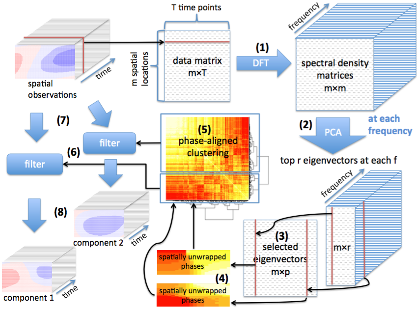
Our proposed phase-aligned spectral filtering method have two main motivations. The first motivation is Brillinger’s dimension reduction strategy for multivariate time series using eigenvalue decomposition applied on the spectral density matrices in the frequency domain [40]. By assembling linear filters based on eigenvectors from different frequencies, we can derive principal component series (PCS) that have zero coherence at all frequencies. This is a desirable properties for further predictive modeling using such series. To maintain the maximal information in the original series while reducing dimensions, eigenvectors corresponding to top eigenvalues are selected from each frequency. Applying a second set of filters constructed using the conjugate of of these selected eigenvectors at different frequencies, the principal component series can be filtered back into lower-rank components of the original data. In [40], it is suggested that the $k$th eigenvector from each frequency be used to assemble the filters for the $k$th component. However, this is not well motivated nor required for having zero coherence among the PCS or the rest of Brillinger’s results in [40]. As our second motivation, in this paper, we identify a link between phase-correlation in spectral densities and a number of low-rank smooth spatiotemporal dynamics. This provides a novel approach for assembling spectral filters that will decompose the original high-dimensional time series into lower-rank spatially smooth dynamic components. The proposed framework follow a sequence of steps as shown in Figure 2.

In the following sections, we explain in details the phase-aligned spectral flitering method, starting with dimension reduction in the frequency domain (Section 2.2), eigenvalue shrinkage (Section 2.3) and reassembling of principle component series (Section 2.4). Section 2.5 explains the computational steps of decomposing a high-dimensional spatiotemporal data set using the proposed phase-aligned spectral filtering method.

Consider a real-valued spatiotemporal process $\{Z_{s,t}\in\mathbb{R}:s\in\mathcal{D}_{m},t\in\mathcal{T}\}$ where the discrete spatial domain $\mathcal{D}_{m}=\{s_{1},...,s_{m}\}\subset\mathcal{D}$ contains a set of $m$ locations and $\mathcal{T}=\{0,\pm 1,\pm 2,\cdots\}$. Assume that $\boldsymbol{Z}_{t}=\{Z_{s,t}:s\in\mathcal{D}_{m}\}$ is a second-order stationary $m$-dimensional vector-valued time series with mean $\boldsymbol{\mu}$ and $m\times m$ spectral density $f_{zz}(\omega)$ for $\omega\in[-\frac{1}{2},\frac{1}{2}]$. Without loss of generality, we assume $\boldsymbol{\mu}=\boldsymbol{0}$. The spectral density matrix $f_{zz}(\omega)$ is a complex-valued positive semidefinite Hermitian matrix in the form of

where $\Gamma(h)$ is the autocovariance function of $\boldsymbol{Z}_{t}$.

Brillinger (1981)[40] stated that for each integer $1\leq r\leq m$, there exist a pair of filters $\{\mathbf{C}^{[r]}_{\tau}\in\mathbb{R}^{r\times m}:u\in\mathcal{T}\}$ and $\{\mathbf{B}^{[r]}_{\tau}\in\mathbb{R}^{m\times r}:u\in\mathcal{T}\}$ that minimizes the mean squared error

where

The sequence of matrices are

where

and $\boldsymbol{v}_{(1)}(\omega),\cdots,\boldsymbol{v}_{(r)}(\omega)$ are the $r$ eigenvectors of $f_{zz}(\omega)$ corresponding to its first $r$ largest eigenvalues $\lambda_{(1)}(\omega),\cdots,\lambda_{(r)}(\omega)$. The resulted $\boldsymbol{X}^{[r]}_{t}$, referred to as principal component series, has a spectral density matrix

which means any pair of the principal component series $X_{k,t}$ and $X_{j,t}$ for $k\neq j$ has zero coherence.

At each frequency, we decompose the spectral density as follows

where $f_{\epsilon\epsilon}(\omega)$ is the spectral density of the error series $\boldsymbol{\epsilon}_{t}=\boldsymbol{Z}_{t}-\tilde{\boldsymbol{Z}}_{t}$. In many cases, the spectral power concentrates in a relatively small area along the frequency axis, that is, if we pool the first $r$ largest eigenvalues at all frequencies, there remain a large proportion of eigenvalues being relatively small, or even close to zero. Here we propose a threshold $\Delta$ and further define

The decomposition of the spectral density of $\boldsymbol{Z}_{t}$ becomes

If $r_{\omega}$ is 0, then $f_{\tilde{z}^{\star}\tilde{z}^{\star}}(\omega)=0$. Compared to the previous filtered series $\tilde{\boldsymbol{Z}}_{t}$, the new filtered series $\tilde{\boldsymbol{Z}}^{\star}_{t}$ is less noisy and more robust. This shrinkage step is also important and necessary in the next phase-aligned reassembling step.

The spectral density of the $r$-dimensional principal component series $\boldsymbol{X}_{t}$’s obtained in (3) is diagonal and aligned in descending order. However, the $k$-th assembled principal component series $X_{k,t}$ that is constructed using the eigenvector corresponding to the $k$-th largest eigenvalue at every frequency lack interpretability. As a matter of fact, given a pool of eigenvectors from different frequencies derived by previous steps, we can reassemble eigenvectors at different frequencies arbitrarily yet still maintain the zero coherence property of the resulting principal component series. The problem we are interested in solving is: given $(\boldsymbol{v}_{(1)}(\omega)$, $\boldsymbol{v}_{(2)}(\omega)$, $\cdots$, $\boldsymbol{v}_{(r)}(\omega))$, how do we assemble principal component series from a pool of eigenvectors at different frequences, so that to have an interpretable decomposition?

We build a solution to the above problem based on the fact that a shift in the time domain corresponds to a phase change in the frequency domain. This change is a linear function of frequency. For example, if a signal is propagating, the observations would take form as decayed and delayed versions of the original signal. Furthermore, if the rate of energy decay and the amount of time delay only depend on the location of observation and the original location of the signal, that is, does not depend on time, the corresponding phase of the Fourier transform of such signals would be perfectly correlated in the frequency domain.

Simple dynamics such as signal propagating and sensing towards mobile energy sources lead to correlated phase in the frequency domain (see proofs in the Appendix). If we cluster eigenvectors with correlated phases to assemble principle component series, the filters constructed from each cluster would produce meaningful and interpretable spatiotemporal dynamics.

In this section, we will outline the steps for the phase-aligned spectral filtering method.

Parameter estimation. In practice, we only have observations on a finite time horizon. Let $\{z_{s,t}\in\mathbb{R}:s\in\mathcal{D}_{m},t\in\mathcal{T}_{n}\}$ denote the observed data where $\mathcal{T}_{n}=\{1,\cdots,n\}\subset\mathcal{T}$. In order to assemble the desired phase-aligned spectral filters as described above, we need to estimate the paired filters $\{\mathbf{C}_{\tau}=(\mathbf{C}_{1,\tau}^{\top},\cdots,\mathbf{C}_{r,\tau}^{\top})^{\top}\in\mathbb{R}^{r\times m}\}$ and $\{\mathbf{B}_{\tau}=(\mathbf{B}_{1,\tau},\cdots,\mathbf{B}_{r,\tau})\in\mathbb{R}^{m\times r}\}$ from this finite sample so that the principal component series

has diagonal or approximately diagonal spectral density and its resulting dynamic component $\tilde{\boldsymbol{z}}^{(k)}_{t}$ obtained from

has correlated phases across frequencies where $1\leq k\leq r$, $\mathbf{C}_{k,\tau}$ is the $k$-th row vector of $\mathbf{C}_{\tau}$ and $\mathbf{B}_{k,\tau}$ is the $k$-th column vector of $\mathbf{B}_{\tau}$.

The paired filters are constructed from the eigenvectors of spectral density matrices $f_{zz}(\omega)$. We estimate the eigenvectors $\boldsymbol{v}_{j}(\omega)$ by the eigenvectors of estimated spectral density $\hat{f}_{zz}(\omega)$. The spectral density matrices at Fourier frequencies $\omega_{j}=j/n$ for $j=0,\cdots,n-1$ are estimated by the smoothed periodogram

where $P(\omega_{j})$ is the raw periodogram and $h_{k}$ is a smoothing kernel of bandwidth equal to $(2q+1)$ satisfying: i) $h_{k}>0$; ii) $\sum^{q}_{k=-q}h_{k}=1$; and iii) $q\rightarrow\infty$ and $q/n\rightarrow 0$, $\sum^{q}_{k=-q}h^{2}_{k}\rightarrow 0$ as $n\rightarrow\infty$.

Phase unwrapping. We obtain the raw phase of the estimated $k$th eigenvector, $\mbox{Arg}(\hat{\boldsymbol{v}}_{k}(\omega_{j}))$ at frequency $\omega_{j}$, by taking logarithm of the estimated eigenvector $\hat{\boldsymbol{v}}_{k}(\omega_{j})$ and extract the imaginary part. However, the resulting phase estimate is only given as the actual phase modulo $2\pi$, between $-\pi$ and $\pi$. Even when the phase vectors of two eigenvectors are completely correlated, such a loss of information will render them much less correlated. In order to carry out our phase-aligned reassembling of eigenvectors, we need to recover the true phase up to a linear transformation.

The computed raw phase (modulo $2\pi$) has discontinuities near $\pi$ and $-\pi$. We assume the true phase is continuous in space. Based on this assumption, we can then unwrap the raw phase values, in other words, resolve the jumps of phase values in a two dimensional space to derive continuous phase values. Over the spatial locations $s_{k}\in\mathbb{R}^{2}$, we apply the two-dimensional phase unwrapping algorithm proposed in [41] to each $\mbox{Arg}(\hat{\boldsymbol{v}}_{k}(\omega))$ for $k=1,\cdots,r_{\omega}$. The algorithm changes the raw values of $\mbox{Arg}(\boldsymbol{v}_{k}(\omega_{j}))$ by adding $2c\pi$ with $c\in\mathbb{Z}$ at jumps so that the unwrapped phase values, denoted by $\widetilde{\mbox{Arg}}(\hat{\boldsymbol{v}}_{k}(\omega_{j}))$ attain a maximum level of continuity over spatial locations.

Phase clustering. On the unwrapped phases $\widetilde{\mbox{Arg}}(\hat{\boldsymbol{v}}_{k}(\omega_{j}))$ of the selected eigenvectors whose eigenvalues $\hat{\lambda}_{k}(\omega_{j})$ are greater than or equal to $\Delta$, we deploy hierarchical clustering as the clustering algorithm with one minus correlation as the distance measure and Ward’s clustering criterion [42] as the linkage agglomeration method.

We then construct filters from each cluster to create reassembled principal component series that correspond to dynamics with correlated phases in their spectral densities. To construct the desired filters from each cluster, we label each of the selected eigenvector by its group number from the unwrapped phase clustering results. And then the paired filters for the $k$-th principal component series and its corresponding dynamic component are constructed by

where $\hat{\boldsymbol{v}}_{k}(\omega_{j})$ is the eigenvector with a group label equal to $k$ when its eigenvalue $\hat{\lambda}_{k}(\omega_{j})$ is greater than or equal to $\Delta$.

The phase-aligned spectral filtering algorithm. The complete phase-aligned spectral filtering decomposition procedure for spatiotemporal dynamics is summarized in Algorithm 1. The step numbers are the same as in Figure 2.

In this example, we create a scenario where the observed value at a given grid location and a given time point is the total energy absorbed by the unit block area centered at this given grid location, from all rotating energy sources.

On the $20\times 20$ grid, there are two energy sources affecting the area, each of which moves following a circular trajectory. The two trajectories are centered at $c^{(1)}_{c}=(15,15)$ and $c_{c}^{(2)}=(5,5)$ respectively, with radius of $r^{(1)}_{c}=r^{(2)}_{c}=5$. The two energy sources move different angular velocities of $v^{(1)}_{\theta}=2\pi/20$ and $v^{(2)}_{\theta}=2\pi/5$ per time unit counterclockwise respectively. The initial positions of the two energy sources on the trajectory circles, denoted by $\theta^{(1)}_{0}$ and $\theta^{(2)}_{0}$ measuring the angular distance from the horizontal axis. They are randomly assigned in each simulation. The $i$-th energy source’s position at $t=0$ can therefore be written as $c^{(i)}_{c}+(r^{(i)}_{c}\cos\theta^{(i)}_{0},r^{(i)}_{c}\sin\theta^{(i)}_{0})$ with $\theta^{(i)}_{0}$ uniformly sampled between $0$ to $2\pi$ for $i=1,2$. At any subsequent time point $t$, the $i$-th energy source’s position is

Assume that the energy absorbed from the energy source decays exponentially in squared distance. For $s\in\mathcal{D},t\in\mathcal{T}_{n}=\{1,2,\cdots,n\}$, we can explicitly write down the energy at location $s$ and time $t$ absorbed from the $i$-th energy sources positioned at $c^{(i)}_{t}$ as

where $E^{(i)}_{0}$ is the total emitted energy of the $i$-th energy source during any unit time. $E^{(i)}_{0}$ is assumed to be a constant for simplicity. The total amount of energy measured at location $s$ and time $t$ is the sum of energy absorbed from all sources, that is,

Thus, the amount of energy the grid block $s_{j,k}$ absorbs at time $t$ is

The total emitted energy $E^{(i)}_{0}$ is set to be $1000$ and the bandwidth parameter $\gamma^{(i)}$ is set to be $5$ for $i=1,2$. We use the demeaned $\boldsymbol{z}^{(1)}_{t}$ and $\boldsymbol{z}^{(2)}_{t}$ as the underlying dynamic systems that affect the grid area. The final observed measurements are the energy distributed by these two rotating sources overlaid and superimposed on each other with high dimensional white noises added, i.e.,

Using vectorized notation for $\varepsilon_{(j,k),t}$, we define $\boldsymbol{\varepsilon}_{t}=(\varepsilon_{1,t},\varepsilon_{2,t},\cdots,\varepsilon_{400,t})^{\top}$. We assume that $\boldsymbol{\varepsilon}_{t}\sim\mathcal{N}(0,\sigma^{2}_{\varepsilon}\mathbf{I}_{m})$ where $m=400$. We set three noise levels in this simulated scenario: low-noise level with $\sigma^{2}_{\varepsilon}=0.16$, mid-noise level with $\sigma^{2}_{\varepsilon}=4$ and high-noise level with $\sigma^{2}_{\varepsilon}=16$. The top three rows of Fig. 3 are the level plots of the two rotating energy sources $\boldsymbol{z}^{(1)}_{t}$ and $\boldsymbol{z}^{(2)}_{t}$ along with the observed data $\boldsymbol{y}_{t}$ from $t=1$ to $t=5$ under the three noise-level settings. As one can see, when $\sigma^{2}_{\varepsilon}$ increases to $16$, the two dynamic systems are barely discernible in the superimposed observed data.

The performance of our phase-aligned spectral filtering (PASF) algorithm was evaluated on the simulated data under these three noise level settings. See Appendix for implementation details. The lower three rows of Fig. 3 display the decomposition results by phase-aligned spectral filtering (PASF) in the low-, mid- and high-noise level settings respectively. Rows 4 and 5 are the identified dynamic components using our proposed method. Under the low-noise setting, the first and second components explain 48% and 47% of the variability in observed data respectively. When $\sigma^{2}_{\varepsilon}=4$ (mid-noise level), each of the two dynamic components accounts for 23% of the data’s variability. When $\sigma^{2}_{\varepsilon}$ increases to 16 (an overwhelmingly high noise level), variability carried by the two filtered components drops to 8%. It can be seen clearly from Fig. 3 that the phase-aligned spectral filtering (PASF) approach is still able to capture and separate the underlying dynamic systems even when the signal to noise ratio drops below $0.1$ (the variance of the signals is approximately $1.6$). Row 6 of each panel displays the residuals after we subtract the filtered components constructed by phase-aligned spectral filtering (PASF), which resemble white noises. See Supplement Information for animated plots of these simulation results.

For comparison, we also applied the principal component analysis (PCA), independent component analysis (ICA), singular spectrum analysis (SSA) [39] and principal component analysis for time series (PCA4TS) [37] to the simulated data from the rotating energy source example. Fig. 4 provides a side-by-side comparison of the decomposition results obtained by phase-aligned spectral filtering (PASF) and these methods found in the literature, under the low-noise level setting with $\sigma^{2}_{\varepsilon}=0.16$. The top left panel displays the ground truth, i.e., the true signals $\boldsymbol{z}^{(1)}_{t}$ and $\boldsymbol{z}^{(2)}_{t}$ that generate the observed data $\boldsymbol{y}_{t}$. The top right panel is the two components as well the residuals from our phase-aligned spectral filtering (PASF) method. The remaining panels are the resulting dynamic components and corresponding residuals computed by the literature methods (See Appendix for implementation details of these literature methods.). Comparison results under the mid- and high-noise level setting can be found in Appendix as Fig. A2 and Fig. A3.

None of the literature methods is able to recover the two underlying dynamic systems as our method does. The dynamics yielded from PCA and ICA are distant from the true dynamics since they can only capture linear features with no time dependence. SSA is able to separate the smooth dynamics from the noisy data but failed to separate them. The performance of PCA4TS is better than PCA and ICA but worse than SSA in the low-noise setting, and behaves more like PCA in the mid- and high-noise level settings.

Animated level plots of these decompositions can be found in Appendix.

The second spatiotemporal system of dynamics considered in our simulation study involves a scenario where multiple signal processes propagate on a grid. Different from the previous scenario, here the signal sources do not move. Rather, the signals propagate along preset directions. Observed value at any spatial location and at a given time $t$ is then the sum of all propagated signals at this location and time. We further assume that the magnitude of signals decays as it propagates. Assume that four independent univariate autoregressive processes, denoted as $X_{k}$ for $k=1,2,3,4$, sit at the four corners of the grid. The observed value at grid block $s_{j}$ for $j=1,\cdots,400$ at time $t$ can be written as the sum of four independent signal processes with different time lags:

where $\{a_{jk},k=1,\ldots,4\}$ are linear weights at location $s_{j}$ for the signals $X_{k}$ and $\{t_{jk},k=1,\ldots 4\}$ are lag delays between $s_{j}$ and $X_{k}$ respectively. Each signal, $\{X_{k,t}\}$, $k=1,\ldots,4$, is an autoregressive process of order 2, that is,

with $\beta_{1,1}=\beta_{2,1}=0.9$, $\beta_{3,1}=\beta_{4,1}=-0.9$, $\beta_{1,2}=\beta_{3,2}=-0.5$, and $\beta_{2,2}=\beta_{4,2}=-0.8$.

Denote the location coordinates for $X_{k,t}$ by $c_{k}$. In our simulation, we use $c_{1}=(0,0)$, $c_{2}=(20,0)$, $c_{3}=(0,20)$ and $c_{4}=(20,20)$. For $Y_{s_{j},t}$, $a_{jk}$ and $t_{jk}$ are decided by the spatial distance between the grid block $s_{j}$ and the location of signals. Specifically,

where $\|\cdot\|_{1}$ and $\|\cdot\|_{2}$ are the $L_{1}$ and $L_{2}$ norm respectively. Parameter $\gamma$ is the signals’ rate of decay when propagating and is set to be 50 in this simulation. The observed value $Y_{s_{j},t}$ is then the sum of four dynamic components $Y_{s_{j},t}^{(1)}$, $Y_{s_{j},t}^{(2)}$, $Y_{s_{j},t}^{(3)}$ and $Y_{s_{j},t}^{(4)}$ where

Let the vectorized notation of the propagating signal over the grid at time $t$ be $\boldsymbol{Y}_{t}^{(k)}=(Y_{s_{1},t}^{(k)},Y_{s_{2},t}^{(k)},\cdots,Y_{s_{400},t}^{(k)})^{\top}$. The top-left panel of Figure 5 displays the true propagating components $\boldsymbol{Y}_{t}^{(1)}$, $\boldsymbol{Y}_{t}^{(2)}$, $\boldsymbol{Y}_{t}^{(3)}$ and $\boldsymbol{Y}_{t}^{(4)}$ along with the aggregated signals as observed data. The estimated variances of the four signals are 2.55, 2.02, 1.14, and 1.09. The top-right panel of Figure 5 displays the dynamic components obtained from the proposed phase-aligned spectral filtering (PASF) method and the corresponding residuals. The corresponding components resulted from our method account for 36%, 31%, 16% and 14% of all variability in the observed data. Although the data do not display any evident patterns or dynamics, our proposed approach still manage to detect and separate the four propagating signals from the very noise-like data.

We also compare our approach with the same four literature methods that were used in the previous example. Figure 5 shows the decomposition results from these methods for comparison. The animated version of these results can be found in the Appendix. As we can see, PCA identifies the direction orthogonal to the direction of signal propagating but fails to capture the dynamics. Other literature methods capture even less than PCA. In this example, only our phase-aligned spectral filtering (PASF) method can almost fully recover the dynamic components corresponding to the four propagating signals.

References

- [1] Christopher K Wikle and Mevin B Hooten. A general science-based framework for dynamical spatio-temporal models. Test, 19(3):417–451, 2010.
- [2] Noel Cressie and Hsin-Cheng Huang. Classes of nonseparable, spatio-temporal stationary covariance functions. Journal of the American Statistical Association, 94(448):1330–1339, 1999.
- [3] Tilmann Gneiting. Nonseparable, stationary covariance functions for space–time data. Journal of the American Statistical Association, 97(458):590–600, 2002.
- [4] Chunsheng Ma. Families of spatio-temporal stationary covariance models. Journal of Statistical Planning and Inference, 116(2):489–501, 2003.
- [5] Christopher K Wikle. Hierarchical bayesian models for predicting the spread of ecological processes. Ecology, 84(6):1382–1394, 2003.
- [6] Michael L Stein. Space–time covariance functions. Journal of the American Statistical Association, 100(469):310–321, 2005.
- [7] Christopher J Paciorek and Mark J Schervish. Spatial modelling using a new class of nonstationary covariance functions. Environmetrics, 17(5):483–506, 2006.
- [8] Thaís CO Fonseca and Mark FJ Steel. A general class of nonseparable space–time covariance models. Environmetrics, 22(2):224–242, 2011.
- [9] Moreno Bevilacqua, Carlo Gaetan, Jorge Mateu, and Emilio Porcu. Estimating space and space-time covariance functions for large data sets: a weighted composite likelihood approach. Journal of the American Statistical Association, 107(497):268–280, 2012.
- [10] Nan-Jung Hsu, Ya-Mei Chang, and Hsin-Cheng Huang. A group lasso approach for non-stationary spatial–temporal covariance estimation. Environmetrics, 23(1):12–23, 2012.
- [11] InKyung Choi, Bo Li, and Xiao Wang. Nonparametric estimation of spatial and space-time covariance function. Journal of Agricultural, Biological, and Environmental Statistics, 18(4):611–630, 2013.
- [12] Knut Solna and Paul Switzer. Time trend estimation for a geographic region. Journal of the American Statistical Association, 91(434):577–589, 1996.
- [13] Christopher K Wikle and Noel Cressie. A dimension-reduced approach to space-time kalman filtering. Biometrika, 86(4):815–829, 1999.
- [14] Hsin-Cheng Huang and Nan-Jung Hsu. Modeling transport effects on ground-level ozone using a non-stationary space–time model. Environmetrics, 15(3):251–268, 2004.
- [15] Ke Xu, Christopher K Wikle, and Neil I Fox. A kernel-based spatio-temporal dynamical model for nowcasting weather radar reflectivities. Journal of the American Statistical Association, 100(472):1133–1144, 2005.
- [16] Alan E Gelfand, Sudipto Banerjee, and Dani Gamerman. Spatial process modelling for univariate and multivariate dynamic spatial data. Environmetrics, 16(5):465–479, 2005.
- [17] Gardar Johannesson, Noel Cressie, and Hsin-Cheng Huang. Dynamic multi-resolution spatial models. Environmental and Ecological Statistics, 14(1):5–25, 2007.
- [18] Fabio Sigrist, Hans R Künsch, and Werner A Stahel. A dynamic nonstationary spatio-temporal model for short term prediction of precipitation. The Annals of Applied Statistics, 6(4):1452–1477, 2012.
- [19] Dan W Gladish and Christopher K Wikle. Physically motivated scale interaction parameterization in reduced rank quadratic nonlinear dynamic spatio-temporal models. Environmetrics, 25(4):230–244, 2014.
- [20] Robert Tibshirani. Regression shrinkage and selection via the lasso. Journal of the Royal Statistical Society. Series B (Methodological), 58(1):267–288, 1996.
- [21] Lewis L Thurstone. Multiple factor analysis. Psychological Review, 38(5):406, 1931.
- [22] Rudolph Emil Kalman. A new approach to linear filtering and prediction problems. Journal of Fluids Engineering, 82(1):35–45, 1960.
- [23] Pierre Comon. Independent component analysis, a new concept? Signal Processing, 36(3):287–314, 1994.
- [24] Karl Pearson. Liii. on lines and planes of closest fit to systems of points in space. The London, Edinburgh, and Dublin Philosophical Magazine and Journal of Science, 2(11):559–572, 1901.
- [25] Ian Jolliffe. Principal component analysis. Wiley Online Library, 2002.
- [26] Harold Hotelling. Analysis of a complex of statistical variables into principal components. Journal of Educational Psychology, 24(6):417, 1933.
- [27] Kari Karhunen. Über lineare methoden in der wahrscheinlichkeitsrechnung. Ann. Acad. Sci. Fennicae. Ser. A. I. Math.-Phys., 37:1–79, 1947.
- [28] Michel Loève. Fonctions aléatoires de second order. In Paul Lévy, editor, Processus Stochastique et Movement Brownien. Hermann, Paris, 1948.
- [29] Edward N Lorenz. Empirical orthogonal functions and statistical weather prediction. Scientific report no.1, Massachusetts Institute of Technology, Department of Meteorology, 1956. Statistical Forecasting Project.
- [30] George EP Box and George C Tiao. A canonical analysis of multiple time series. Biometrika, 64(2):355–365, 1977.
- [31] Peter CM Molenaar. A dynamic factor model for the analysis of multivariate time series. Psychometrika, 50(2):181–202, 1985.
- [32] Andrew D Back and Andreas S Weigend. A first application of independent component analysis to extracting structure from stock returns. International Journal of Neural Systems, 8(04):473–484, 1997.
- [33] Mario Forni, Marc Hallin, Marco Lippi, and Lucrezia Reichlin. The generalized dynamic-factor model: Identification and estimation. Review of Economics and Statistics, 82(4):540–554, 2000.
- [34] James H Stock and Mark W Watson. Forecasting using principal components from a large number of predictors. Journal of the American Statistical Association, 97(460):1167–1179, 2002.
- [35] David S Matteson and Ruey S Tsay. Dynamic orthogonal components for multivariate time series. Journal of the American Statistical Association, 106(496):1450–1463, 2011.
- [36] Zhaoran Wang, Fang Han, and Han Liu. Sparse principal component analysis for high dimensional multivariate time series. In Proceedings of the Sixteenth International Conference on Artificial Intelligence and Statistics, volume 31, pages 48–56, 2013.
- [37] Jinyuan Chang, Bin Guo, and Qiwei Yao. Segmenting multiple time series by contemporaneous linear transformation. arXiv preprint arXiv:1410.2323, 2014.
- [38] Mario Forni, Marc Hallin, Marco Lippi, and Paolo Zaffaroni. Dynamic factor models with infinite-dimensional factor spaces: One-sided representations. Journal of Econometrics, 185(2):359–371, 2015.
- [39] Michael Ghil, MR Allen, MD Dettinger, K Ide, D Kondrashov, ME Mann, Andrew W Robertson, A Saunders, Y Tian, F Varadi, and P Yiou. Advanced spectral methods for climatic time series. Reviews of Geophysics, 40(1):3–1–3–41, 2002.
- [40] David R Brillinger. Time series: data analysis and theory. Holden-Day, 1981.
- [41] Miguel Arevallilo Herráez, David R Burton, Michael J Lalor, and Munther A Gdeisat. Fast two-dimensional phase-unwrapping algorithm based on sorting by reliability following a noncontinuous path. Applied Optics, 41(35):7437–7444, 2002.
- [42] Joe H Ward Jr. Hierarchical grouping to optimize an objective function. Journal of the American Statistical Association, 58(301):236–244, 1963.
- [43] Eugenia Kalnay, Masao Kanamitsu, Robert Kistler, William Collins, Dennis Deaven, Lev Gandin, Mark Iredell, Suranjana Saha, Glenn White, and John Woollen. The ncep/ncar 40-year reanalysis project. Bulletin of the American Meteorological Society, 77(3):437–471, 1996.
Appendix A1 Computation details for examples
Rotating energy source examples.
For applying phase-aligned spectral filtering (PASF) to the rotating energy source examples, the bandwidth of the Daniell kernel used for smoothing the raw periodogram is chosen to be . The threshold is decided by the spectral gap in the pooled eigenvalues. The total number of selected eigenvectors is for the low- and mid-noise cases and for the high-noise case.
For PCA and ICA, we extract the first two components with highest energy, that is, the two components corresponding to the first two largest eigenvalues.
For SSA, the first 10 largest singular values are dominant in the low- and mid-noise level settings. In the high-noise setting, the gap appears between the eighth and ninth largest singular values. We divide the corresponding components into two groups by clustering them based on their weighted correlation and reconstruct the final two components from each group. The weighted correlation is a measure of the degree of separability between two series and defined as
where , , , and both of the two series and have a time length equal to .
For PCA4TS, we choose the two groups whose corresponding components in the original space have largest variance.
Signal propagation examples.
The bandwidth of the Daniell kernel for smoothing the raw periodogram is chosen to be . The total number of selected eigenvectors is 1000 and the dendrogram displays four clean clusters. The resulting components obtained from our algorithm show evident dynamics of four processes propagating on the grid area which perfectly correspond to the generated signals.
We extract the first four components for the PCA and ICA respectively. For SSA, we divide the first 50 components into four groups by clustering them based on their weighted correlation and reconstruct one new component from each group. For PCA4TS, we choose the four groups whose corresponding components in the original space have the largest variance.
Real data analysis: sea level pressure.
The observations were first demeaned for each location before analysis. The bandwidth of the Daniell kernel for smoothing the periodogram was chosen to be 21. The total number of selected eigenvectors is 2000 and the resulting number of clusters is 2.
As in the simulation examples, we extract the first two components from PCA and ICA. We cluster the components from SSA into two groups based on their weighted correlation to obtain two final additive components. We select the first two components with the largest variance from PCA4TS.
Appendix A2 Connecting phase correlation with simple spatiotemporal dynamics
In this section we show that two common spatiotemporal dynamics can create phase correlation between their spectral densities at different frequencies.
A2.1 Signal Propagation
Assume that there are independent real-valued signal processes propagating and the observed process satisfies
where and the spectral density of is
Then the element of the spectral density of in the -th row and -th column is given by
If we define
then . The phase of is which is a linear function of .
A2.2 Rotating Energy Source
Consider a mobile energy source defined by where is the rotating trajectory and is the energy it carries at time . Assume that orbits around a center with uniform angular speed . That is,
where is the initial angle and is the distance between and .
Now consider the observation being the absorbed energy from the signal at location and time where can be written as
Assume that is in the form of
where is a non-negative real-valued monotone decreasing function satisfying , and is the Euclidean distance between and , that is,
We assume for stationarity, that is, does not change over time. Let
and be the Fourier Transform of . Then the Fourier Transform of is
Since is a symmetric function of , is real. Therefore the modulus of is and the phase
is a linear function of .
Appendix A3 Additional figures