Low-energy Spin Dynamics of the Honeycomb Spin Liquid Beyond the Kitaev Limit

Quantum spin liquids (QSLs) have attracted wide attention due to their intriguing highly entangled nature and exotic properties [1, 2]. Amongst the simplest and most interesting QSLs are those with intrinsic topological order, which are of particular interest as potential platforms for quantum computing possessing intrinsic protection from decoherence[3]. A prominent feature of topological phases and QSLs in general is the fractionalization of electrons or spins into other particles, Majorana fermions for example. An unequivocal observation of this fractionalization is a key goal of the QSL field.

Recent theory and experiment have unveiled the exciting prospect of achieving this objective in highly anisotropic spin-1/2 magnets on honeycomb lattices, including Na₂IrO₃, Li₂IrO₃, and $\alpha$-RuCl₃[4, 5, 6, 7, 8, 9, 10, 11, 12, 13, 14, 15, 16]. Two key theoretical works presaged this experimental venue. First, a seminal paper by Kitaev[17] introduced a simple near-neighbor spin Hamiltonian on this lattice, possessing a gapless $\mathbb{Z}_{2}$ QSL phase, the excitations of which are massless relativistic (i.e. linearly dispersing) Majorana fermions and gapped bosonic ‘‘fluxes’’¹¹ 1 Kitaev also demonstrated other phases in the limits of strong anisotropy and upon application of a particular orientation of magnetic field. This is, however, not relevant to our discussion.. Second, Jackeli and Khaliullin[19] showed that Kitaev’s anisotropic interactions arises naturally from certain superexchange processes in strongly spin-orbit coupled transition metal compounds. These two developments spurred the search for Kitaev’s QSL in this context in the laboratory.

In this paper, we address a key experimental signature of any magnet, the dynamical spin structure factor, for the Kitaev QSL. The dynamic spin response can be measured using conventional experiment techniques such as inelastic neutron scattering and electron spin resonance. It is given, at zero temperature, by

where $\sigma^{\mu}_{i}$ is the Pauli operator representing the $\mu^{\rm th}$ component of the spin at site $i$ of the lattice, and the arguments indicate the usual Heisenberg time evolution. Previous studies demonstrated that for Kitaev’s exactly soluble model $S^{\mu\nu}_{ij}$ vanishes between all but the neighbor pair of spins [20]. Moreover, the dynamical spin response exhibits a spin gap – a non-zero interval of frequency around zero in which the spectral weight vanishes – despite the existence of gapless excitations [21, 22]. These remarkable properties arise due to the exact integrability of the Kitaev model. Here we ask the important question whether the apparent spin gap persists when moving away from the exactly solvable point in the critical spin liquid phase[23, 24]. We find that the existence of the gap as a robust property of the QSL phase relies critically upon internal symmetries: it is present in the Heisenberg-Kitaev model but not in the generic model allowed by physical symmetries in actual materials. In the latter case we obtain universal power-law spectral weight at low energies, as shown in Figs. 2, 3. This, rather than the gap found in Ref.21, is the expected behavior should the Kitaev QSL be realized in actual experiments.

To obtain these results, we follow standard arguments of low energy effective field theory. The low energy field theory in the gapless phase of Kitaev model is a single cone of massless Dirac fermions (a convenient formulation for two Majorana cones). Physical operators may be expanded in the primary field and descendents of the field theory, here the Dirac fields, and we expect all terms consistent with symmetry to generically appear in this expansion. Due to the fine-tuned nature of the exactly soluble point, many coefficients in this expansion vanish there, but will become non-zero if symmetry allows. In the case of a QSL phase, the analysis of permitted terms is subtler because the physical symmetries are intertwined with emergent gauge transformations of the non-local fermions. This is described by the mathematical structure of projected symmetry groups (PSGs)[25, 26, 27, 28, 29]. Here, we use the PSG analysis of Ref.29 to find the low energy contributions to the microscopic spin operator, and from this deduce the dynamical spin correlations. To complement the PSG analysis, we also study the problem directly by perturbation theory away from the soluble Kitaev point, thereby obtaining the scaling of the prefactors $f_{j}$’s in Eq. (5) of the symmetry-allowed terms.

We begin by recapitulating Kitaev’s model and its solution. It consists of interacting spin-1/2 moments on a honeycomb lattice. Original hamiltonian reads

where $\langle ij\rangle^{\mu}$ denotes the neighbor sites $i,j$ whose bond direction is labeled by $\mu=x,y,z$ (Fig. 1(a)). There is a local conserved quantity for each plaquette $W_{p}=\sigma^{x}_{1}\sigma^{z}_{2}\sigma^{y}_{3}\sigma^{x}_{4}\sigma^{z}_{5}\sigma^{y}_{6}$ (Fig. 1(a)), the set of which on all plaquettes is a set of good quantum numbers labeling energy eigensectors. We say a $\pi$-flux is present on a plaquette $p$ if $W_{p}=-1$. The solution to Kitaev model is well known through the mapping to a free fermion Hamiltonian

if we write each spin as the product of Majorana operators $\sigma^{a}_{i}=\mathrm{i}c_{i}c_{i}^{\mu}$ (physical subspace satisfies $c_{i}c_{i}^{x}c_{i}^{y}c_{i}^{z}=1$) and define bond operator $\hat{u}_{\langle ij\rangle^{\mu}}=\mathrm{i}c^{\mu}_{i}c^{\mu}_{j}$. The bond operators with eigenvalues $\pm 1$ commute with the Hamiltonian and the product of them around a plaquette $p$ is $W_{p}$. Identifying the eigenvalue of $\hat{u}_{\langle ij\rangle^{\mu}}$ as $\mathbb{Z}_{2}$ gauge field, one can obtain the ground state that exists in the zero-flux subspace by setting $\hat{u}_{\langle ij\rangle^{\mu}}$’s to 1 and diagonalizing the Hamiltonian. Complementary to the static flux sector, the Majorana fermions $c_{i}$’s living on-site span the matter fermion (spinon) sector.

From this structure, the short-range and gapped nature of the spin correlations for the soluble model follows directly. When applying a spin operator to the ground state, a spinon excitation is created with two fluxes (illustrated in Fig. 1(a) in green). For $\mathbb{Z}_{2}$ topological order, there are two bosonic anyons, e and m, corresponding to fluxes, and one fermionic anyon, $\varepsilon$, which is the $c_{i}$ fermion. In this language, $\sigma\sim{\sf e}{\sf m}\varepsilon$, which is consistent with general rules since $\varepsilon$ carries both “electric” and “magnetic” gauge charge making the combination of three anyons gauge invariant. Thus a spin gap appears since there is a finite energy difference between the ground state and the lowest eigenstate of the two-vison sector. Infinitely massive visons render the spin correlators short-ranged. Yet both properties may be changed if contributions to the spin of the form $\sigma\!\sim\!\varepsilon\varepsilon$ arise, which appears natural based on the gauge structure alone. To see how they arise, we first consider the structure of states and operators under perturbations, then turn to a general symmetry based analysis.

Unitary transformation analysis: Perturbation theory defines a unitary mapping $U=e^{\mathrm{i}S}$ from eigenstates of the pure Kitaev model $H_{0}$ to those of the perturbed one $H=H_{0}+V$, for example the exact ground state $|\psi\rangle=U|\psi_{0}\rangle$, where $|\psi_{0}\rangle$ is the unperturbed ground state. One can find $U$ order by order by demanding that the rotated Hamiltonian $\tilde{H}=UHU^{-1}$ has vanishing off-diagonal matrix elements between low-energy eigenstates of $H_{0}$, e.g. to first order $\mathrm{i}S=\sum_{n\neq m}\frac{P_{n}VP_{m}}{E_{n}-E_{m}}$, where $P_{n}$ is the projection operator onto the $n$th energy eigenspace. Formally the higher order terms can be found using Baker-Hausdorff formula: they involve more powers of $V$ separated by projection operators and the corresponding energy differences in the denominators. Because the energies of eigenstates of $H_{0}$ with non-uniform fluxes are non-trivial, we are not able to evaluate this explicitly. However, we can understand the general structure of the expansion. Moreover, because the Kitaev QSL is a stable phase, $U$ is well-behaved and $S$ defined in this way is a sum of quasi-local operators, at least when restricted to act (on the right) on low energy states.

In general, we can separate any physical operator, including $U$, into a sum of terms which modify the flux on $2k$ sites: $U=\sum_{k=0}^{\infty}U_{2k}$, where, since $U$ is physical, only an even number of fluxes can be changed. We may understand $U_{2k}$ as the mixing $2k$ virtual fluxes into the interacting ground state.

Spin operators transform accordingly under this procedure:

We observe that since $\sigma_{i}^{\mu}$ modifies two fluxes, terms with $|k-k^{\prime}|=0,1$ induce contributions to $\tilde{\sigma}_{i,0}^{\mu}$. The physical picture behind is that the exact ground state of the perturbed system contains terms with two virtual fluxes, which are annihilated by the spin operator. The resulting state is no longer orthogonal to all the exact zero flux eigenstates. Thus the transformed spin operator has an expression of the form (Fig. 1(b))

where $Z=1$ for the ideal Kitaev model but is reduced by perturbation. All other terms become non-zero with perturbations. The first set of bracketed terms create fluxes exciting modes above a finite energy threshold. We concern here the latter terms, which consist of matter fermions alone and hence create no fluxes and induce only low-energy excitations.

Generic spin operator form from symmetry and gauge constraints: We first consider the constraints on the terms which may arise, focusing on the maximal physical symmetry group generated by the following operations: translations along two basis directions ($T_{1},T_{2}$), time reversal($\mathcal{T}$), $C_{6}$ (a 6-fold rotation plus mirror reflection across honeycomb plane) and $\sigma$ symmetry (mirror reflection across the line orthogonal to the z-bond) (Fig. 1(a), c.f. Ref. 29). In addition, we adopt $h_{x}$ symmetry (a $\pi$ rotation around the direction of x-bond, equivalent to $\sigma C_{6}$). The transformation of Majorana operators should conform to the symmetry enriched topological order of the Kitaev spin liquid, described by PSGs[29].

With these symmetries, we construct combinations of matter fermions compatible with the transformations of spin operators. A basic constraint is gauge invariance imposed on any physical operator. The $\mathbb{Z}_{2}$ gauge transformation induced by $\eta_{i}=\pm 1$ takes $u_{\langle ij\rangle}\rightarrow\eta_{i}u_{\langle ij\rangle}\eta_{j}$ and $c_{i}\rightarrow\eta_{i}c_{i}$. Any product of an even number of matter fermions $c_{i}$, while not gauge invariant on its own, can be made so by multiplying it by a string operator ${\mathcal{U}}_{i_{1}i_{2}}=\prod_{j:i_{1}\rightarrow i_{2}}\hat{u}_{\langle j_{n},j_{n+1}\rangle}$, connecting sites $i_{1},i_{2}$ of Majorana fermions. It is possible to uniquely restore strings in the low energy Hilbert space with $W_{p}=+1$, so in the following we adopt a notation with implicit strings (they can be readily restored when desired).

Having understood gauge invariance, we consider the symmetry transformations of matter fermion products. Consider first time-reversal, under which matter fermion operators on the $A$ sublattice are invariant but those on the $B$ sublattice change sign[29]. Since a spin is odd under $\mathcal{T}$, a corresponding product should consist of an even/odd number of matter fermions on each sublattice if the total number of fermions satisfies $N\equiv 2/0\!\mod\!{4}$, respectively (note the imaginary unit needed when $N\equiv 2\!\mod\!{4}$ to ensure hermiticity).

Thus the smallest appropriate number of matter fermions is two, which must live on the same sublattice. Taking into account the cyclic structure of spin components (which permute under rotations) and the antisymmetry of fermion bilinears, we postulate the form (See Fig. 1(b))

Here $\hat{\mu}$ is the vector in the $\mu$ direction from the A to B site, and $s_{i}=+1(-1)$ for the A (B) sublattice. It is straightforward to check(Appendix A ²² 2 See supplementary material for the discussion on general low-energy forms of spins and the illustration of the flux change in perturbation analysis for specific kinds of perturbations.)that this form is consistent with all the symmetries. Restoring the gauge string connecting sites $i+s_{i}\hat{\nu}$ and $i+s_{i}\hat{\lambda}$, we obtain a gauge invariant expression which can be rewritten in terms of bare spin operators, to wit

Though this operator involves three spins, it is quadratic in the fermions and is expected to give the largest low energy contribution. Terms with more fermion operators or from further separated sites that give subdominant contributions, are discussed in the Appendix A.

We proceed to check how the form arises in perturbation theory. Consider the effect of two perturbations on the Kitaev model[31, 32, 16, 4], namely the Heisenberg interaction $V_{H}=J_{H}\sum_{\langle ij\rangle}{\bm{\sigma}}_{i}\cdot{\bm{\sigma}}_{j}$ and the “cross” term $V_{c}=J_{c}\sum_{\mu(\nu\gamma)}\sum_{\langle ij\rangle^{\mu}}(\sigma^{\nu}_{i}\sigma^{\gamma}_{j}+\sigma^{\gamma}_{i}\sigma^{\nu}_{j})$ ($\nu,\gamma$ are the remaining directions). With either one of the above terms, one can show accidental symmetries cause the spin gap to remain unbroken (i.e. $f$$=$$0$) – see Appendix B. However, when both are present, we find that the contribution in Eq. (7) is induced at fourth order. Specifically, the sequence of two $J_{H}$ and two $J_{c}$ perturbations induces the product $\sigma_{2}^{y}\sigma_{3}^{z}\sigma_{1}^{x}\sim(\sigma_{1}^{x}\sigma_{2}^{x})(\sigma_{1}^{x}\sigma_{2}^{z})(\sigma_{1}^{x}\sigma_{3}^{x})(\sigma_{1}^{x}\sigma_{3}^{y})\sigma_{1}^{x}$. From this, we estimate that the factor $f$ in Eq. (6) scales as $\frac{J_{H}^{2}J_{c}^{2}}{J_{K}^{4}}$.

Low-energy weight of the dynamical spin structure factor: With the low-energy component of the spin operator identified in Eq. (6), we can calculate its contribution to the dynamical spin structure factor $S_{ab}^{\mu\mu}(\bm{q},\omega)\equiv\frac{1}{N}\sum_{i,j}\int_{-\infty}^{+\infty}\mathrm{d}tS_{ia,jb}^{\mu\mu}(t)e^{\mathrm{i}\omega t-\mathrm{i}{\bm{q}}\cdot({\bm{r}}_{i}-{\bm{r}}_{j})}$, where $N$ is the number of unit cells in the lattice. We refine the definition of Eq. (1) by introducing the sublattice indices $a,b=A,B$ apart from the unit cell indices $i,j$. In this section, we will show that the low-energy weight of the spin correlators exhibits power law behavior in frequency. The single-particle spectrum of spinons in the zero-flux sector is $E(\bm{q})=|s_{\bm{q}}|$ where $s_{\bm{q}}=J_{K}(1+e^{\mathrm{i}\bm{q}\cdot\bm{n}_{2}}+e^{-\mathrm{i}\bm{q}\cdot\bm{n}_{1}})$ ($\bm{n}_{1}$, $\bm{n}_{2}$ are basis vectors in Fig. 1(a)). There are two Majorana cones located at the $K$ and $K^{\prime}$ points ($\pm\bm{q}_{0}$) at the Brillouin zone corners, which can be combined into a single cone of Dirac fermions. Expanding the matter fermion field around the Dirac point, we can write

where $\psi_{a}(\bm{r})$ is a slowly varying Dirac field (we take $\bm{r}$ to lie at the hexagon center, i.e. ${\bm{r}}_{i}={\bm{r}}+\hat{x}$ for $i\in A$ and ${\bm{r}}_{i}={\bm{r}}-\hat{y}$ for $i\in B$). Inserting this into the Hamiltonian in Eq. (3) and gradient expanding, we obtain the low-energy dynamics of matter fermions described by the action

where $\psi=(\psi_{A},\psi_{B})^{\intercal}$ and the Fermi velocity $v=\sqrt{3}J_{K}/2$ (The definition of coordinates is indicated in Fig. 1(a)). The field theory is conformally invariant, and the fermion fields scale with length $L$ as $\left[\psi(\bm{r},\tau)\right]=L^{-1}$. We can decompose the low energy spin operator in Eq. (6) similarly using Eq. (8). With some algebra, we obtain the form

where $m_{a}$ and $\bm{n}_{a}^{\mu}$ are two-by-two diagonal matrices, and we used $2{\bm{q}}_{0}=-{\bm{q}}_{0}$ up to a reciprocal lattice vector. Simple specific forms for these matrices in terms of $f$ and ${\bm{q}}_{0}$ are obtained by starting with Eq. (6), but we expect them to be renormalized generally by higher order terms. Both the simple and general symmetry-allowed forms are given in the Appendix A. Note the presence of the gradient in $\hat{N}^{\mu}_{a}$: this cannot be avoided because time-reversal symmetry requires the sublattice degrees of freedom be in a symmetric state, so that the Pauli exclusion principle for this two-particle creation operator forces the orbital wave function to be odd parity; no such requirement applies to the density operator $\hat{M}_{a}^{\mu}$.

At this point, the scaling of low energy spin correlations is evident. Using the dimension of $\psi$, the two-point functions of $\hat{M}_{a}^{\mu}$ and $\hat{N}_{a}^{\mu}$ scale as $\frac{1}{L^{4}}$ and $\frac{1}{L^{6}}$, respectively. The Fourier transformation in 2+1 dimensions adds 3 powers of $L$$\sim$$\frac{1}{\omega}$, so that $S({\bm{q}}$$\approx$$0,\omega)$$\sim$$|\omega|$ corresponding to $\hat{M}_{a}^{\mu}$ correlations, and $S({\bm{q}}$$\approx$$\pm{\bm{q}}_{0},\omega)$$\sim$$|\omega|^{3}$ corresponding to $\hat{N}_{a}^{\mu}$ correlations.

Beyond scaling one obtains the exact low-energy forms by calculation in reciprocal space ($\mu\mu,ab$ are suppressed):

where $|\bm{k}|$$\ll$$|{\bm{q}}_{0}|$. The aforementioned scaling follows immediately using $G(\bm{k},\mathrm{i}\omega_{n})$$\equiv$$-\langle\psi\psi^{\dagger}\rangle_{\bm{k},\omega_{n}}$$=$$\frac{1}{\mathrm{i}\omega_{n}-v\bm{\sigma}\cdot{\bm{k}}}$, which is of dimension $\frac{1}{\omega}$, by rescaling $\bm{k}_{1}(\omega_{1})$$\rightarrow$$\frac{\bm{k}_{1}}{\omega_{n}}(\frac{\omega_{1}}{\omega_{n}})$. One obtains $S(\bm{k},\mathrm{i}\omega_{n})$$\sim$$|\omega_{n}|\tilde{\mathcal{S}}(\frac{v\bm{k}}{|\omega_{n}|})$ and $S(\bm{q}_{0}+\bm{k},\mathrm{i}\omega_{n})$$\sim$$|\omega_{n}|^{3}\tilde{\mathcal{S}}(\frac{v\bm{k}}{|\omega_{n}|})$.

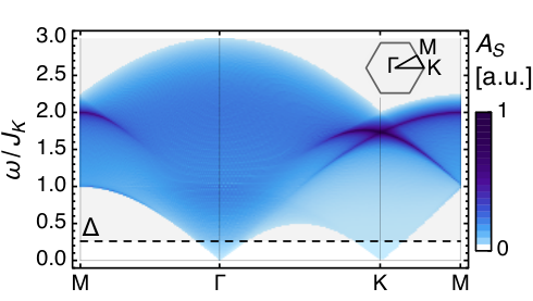
Fig. 2 shows the numerical results of spectral function $A_{S}(\bm{q},\omega)$$=$$-\sum_{\mu}$$\sum_{a,b}2\text{Im}[S^{\mu\mu}_{ab}(\bm{q},\omega+\mathrm{i}0_{+})]$ calculated based on the simple forms for $m_{a}$ and $\bm{n}_{a}^{\mu}$ at the isotropic point. One observes zero low energy spectral weight outside “Dirac cones” centered at $\Gamma$ and $K$, i.e. for $\omega$$<$$v|\bm{k}|$. Direct inspection of the frequency dependence in Fig. 3 confirms the expected $\omega$ and $\omega^{3}$ behaviors at $\Gamma$ and $K$, respectively. Besides this dominant contribution, there will be additional ones arising from products of more than two matter fermion operators, which give larger powers of frequency since every $\psi$ field adds one $\omega$ factor by dimensional analysis. Away form the isotropic limit, i.e. coupling strengths are unequal on bonds for different directions, the Majorana points $\pm{\bm{q}}_{0}$ will be shifted away from the Brillouin zone corners, but the scaling of low energy spin correlations, $S(\bm{q}$$\approx$$0,\omega)$$\sim$$|\omega|$ and $S(\bm{q}$$\approx$$\pm 2\bm{q}_{0},\omega)$$\sim$$|\omega|^{3}$ still hold, since $\mathcal{T}$ still dictates that two-fermion product contains sites on the same sublattice.

The spectral function $S(\bm{q},\omega)$ is of course measured by inelastic neutron scattering. It also describes the longitudinal nuclear spin relaxation rate $\frac{1}{T_{1}}$ in a nuclear magnetic resonance (NMR) experiment, in which $\frac{1}{T_{1}}$ is proportional to the local spectral density of spin fluctuations, which is the momentum integral of $S(\bm{q},\omega)$, with $\omega$ at the (low) NMR frequency. This work predicts temperature scaling $\frac{1}{T_{1}}$$\sim$$T^{3}$, in contrast to the ideal Kitaev spin liquid, where the relaxation rate follows the activated behavior $\sim$$e^{\frac{-\Delta}{T}}$ due to the spin gap $\Delta$. Finally, our result for the uniform component of the spin operator corresponds, if summed over all sites, to the mass term introduced by Kitaev[17] that upon introducing a magnetic field, converts the gapless spin liquid to a gapped non-abelian one. For the soluble model, this gap is cubic in the applied field and appears only if the field couples to all three spin components. Our result implies that, generically, the induced gap is linear in the field and exists for any field orientation.

Conclusion: We showed that generically the low-energy spectral weight of spin structure factor in the gapless Kitaev QSL phase on honeycomb lattice is non-vanishing, in contrast to the special case of the soluble point. The results illustrate a general effective field theory approach, which could be applied to any gapless QSL based on a PSG analysis. In particular for the Kitaev spin liquid we find spectral weight linear (cubic) in $\omega$ near the origin (zone boundary) in momentum space, filling a Dirac-cone-like structure with a sharp spectral edge. These predictions, and not those of the exactly soluble model, describe the proper low energy behavior of any Kitaev spin liquids which might be found experimentally. We note that some previous works[23, 24] have discussed the appearance of power-law correlations upon perturbing the Kitaev model, but our results are distinct and more general.³³ 3 Ref.[23] considered only effects of a field. Ref.[24] showed the absence of low-energy weight for the Heisenberg perturbation, but otherwise gave an incomplete criterion for lifting the gap and did not obtain the effective low energy spin operator or its correlations. It would be interesting to test these predictions numerically, e.g. by DMRG calculations (One can include a term $H^{\prime}$$=$$\Delta\sum_{p}W_{p}$ to raise the flux gap by $\Delta$$>$$0$ and open a larger window to observe the low energy weight).

Acknowledgements. X.-Y. Song thanks G. Khaliullin, F. Wang and G. Halász for helpful discussions. This work was supported by the NSF grant no. DMR-15-06119 (L.B.), the David and Lucile Packard foundation (Y.Y.), the School of Physics at PKU and the 973 Program grant No. 2014CB920902 (X.-Y.S) and benefitted from the facilities of the KITP, supported by NSF grant PHY11-25915.

*

References

- [1] L. Savary and L. Balents, arXiv preprint arXiv:1601.03742 (2016).
- [2] L. Balents, Nature 464, 199 (2010).
- [3] A. Y. Kitaev, Annals of Physics 303, 2 (2003).
- [4] H.-C. Jiang, Z.-C. Gu, X.-L. Qi, and S. Trebst, Phys. Rev. B 83, 245104 (2011).
- [5] J. Reuther, R. Thomale, and S. Trebst, Phys. Rev. B 84, 100406 (2011).
- [6] J. Knolle, G.-W. Chern, D. L. Kovrizhin, R. Moessner, and N. B. Perkins, Phys. Rev. Lett. 113, 187201 (2014a).
- [7] H.-S. Kim, V. S. V., A. Catuneanu, and H.-Y. Kee, Phys. Rev. B 91, 241110 (2015).
- [8] Z. Alpichshev, F. Mahmood, G. Cao, and N. Gedik, Phys. Rev. Lett. 114, 017203 (2015).
- [9] L. J. Sandilands, Y. Tian, K. W. Plumb, Y.-J. Kim, and K. S. Burch, Phys. Rev. Lett. 114, 147201 (2015).
- [10] K. W. Plumb, J. P. Clancy, L. J. Sandilands, V. V. Shankar, Y. F. Hu, K. S. Burch, H.-Y. Kee, and Y.-J. Kim, Phys. Rev. B 90, 041112 (2014).
- [11] K. A. Modic, T. E. Smidt, I. Kimchi, N. P. Breznay, A. Biffin, S. Choi, R. D. Johnson, R. Coldea, P. Watkins-Curry, G. T. McCandless, J. Y. Chan, F. Gandara, Z. Islam, A. Vishwanath, A. Shekhter, R. D. McDonald, and J. G. Analytis, Nat Commun 5 (2014).
- [12] T. Takayama, A. Kato, R. Dinnebier, J. Nuss, H. Kono, L. S. I. Veiga, G. Fabbris, D. Haskel, and H. Takagi, Phys. Rev. Lett. 114, 077202 (2015).
- [13] A. Banerjee, C. A. Bridges, J. Q. Yan, A. A. Aczel, L. Li, M. B. Stone, G. E. Granroth, M. D. Lumsden, Y. Yiu, J. Knolle, S. Bhattacharjee, D. L. Kovrizhin, R. Moessner, D. A. Tennant, D. G. Mandrus, and S. E. Nagler, Nat Mater advance online publication, (2016).
- [14] Y. Singh and P. Gegenwart, Physical Review B 82, 064412 (2010).
- [15] S. Choi, R. Coldea, A. Kolmogorov, T. Lancaster, I. Mazin, S. Blundell, P. Radaelli, Y. Singh, P. Gegenwart, K. Choi, et al., Physical review letters 108, 127204 (2012).
- [16] Y. Singh, S. Manni, J. Reuther, T. Berlijn, R. Thomale, W. Ku, S. Trebst, and P. Gegenwart, Phys. Rev. Lett. 108, 127203 (2012).
- [17] A. Kitaev, Annals of Physics 321, 2 (2006).
- [18] Kitaev also demonstrated other phases in the limits of strong anisotropy and upon application of a particular orientation of magnetic field. This is, however, not relevant to our discussion.
- [19] G. Jackeli and G. Khaliullin, Physical Review Letters 102, 017205 (2009).
- [20] G. Baskaran, S. Mandal, and R. Shankar, Phys. Rev. Lett. 98, 247201 (2007).
- [21] J. Knolle, D. Kovrizhin, J. Chalker, and R. Moessner, Physical Review Letters 112, 207203 (2014b).
- [22] J. Knolle, D. L. Kovrizhin, J. T. Chalker, and R. Moessner, Phys. Rev. B 92, 115127 (2015).
- [23] K. S. Tikhonov, M. V. Feigel’man, and A. Y. Kitaev, Phys. Rev. Lett. 106, 067203 (2011).
- [24] S. Mandal, S. Bhattacharjee, K. Sengupta, R. Shankar, and G. Baskaran, Phys. Rev. B 84, 155121 (2011).
- [25] T. Senthil and M. P. A. Fisher, Phys. Rev. B 62, 7850 (2000).
- [26] L. Balents, L. Bartosch, A. Burkov, S. Sachdev, and K. Sengupta, Phys. Rev. B 71, 144508 (2005).
- [27] T. Senthil and P. A. Lee, Phys. Rev. B 71, 174515 (2005).
- [28] M. J. Lawler, A. Paramekanti, Y. B. Kim, and L. Balents, Phys. Rev. Lett. 101, 197202 (2008).
- [29] Y.-Z. You, I. Kimchi, and A. Vishwanath, Physical Review B 86, 085145 (2012).
- [30] See supplementary material for the discussion on general low-energy forms of spins and the illustration of the flux change in perturbation analysis for specific kinds of perturbations.
- [31] J. c. v. Chaloupka, G. Jackeli, and G. Khaliullin, Phys. Rev. Lett. 105, 027204 (2010).
- [32] J. G. Rau, E. K.-H. Lee, and H.-Y. Kee, Phys. Rev. Lett. 112, 077204 (2014).
- [33] Ref.[23] considered only effects of a field. Ref.[24] showed the absence of low-energy weight for the Heisenberg perturbation, but otherwise gave an incomplete criterion for lifting the gap and did not obtain the effective low energy spin operator or its correlations.