跳到论文正文
W Papers独立论文阅读器 arXiv:1604.04091 论文正文 计算阅读时间 · 0%
引用这篇论文根据当前论文元数据生成,正式投稿前建议核对。


License: arXiv.org perpetual non-exclusive license
arXiv:1604.04091v1 [math.CA] 14 Apr 2016

Boundedness of the density normalised Jones’ square function does not imply 11-rectifiabilityThanks: H.M. is supported by the Academy of Finland through the grant Multiparameter dyadic harmonic analysis and probabilistic methods. T.O. is supported by the Academy of Finland through the grant Restricted families of projections and connections to Kakeya type problems. Both authors are members of the Finnish Centre of Excellence in Analysis and Dynamics Research.

Henri Martikainen and Tuomas Orponen Address: University of Helsinki, Department of Mathematics and Statistics Email address: henri.martikainen@helsinki.fi, tuomas.orponen@helsinki.fi
Abstract.

Recently, M. Badger and R. Schul proved that for a 11-rectifiable Radon measure μ\mu, the density weighted Jones’ square function

J1​(x)=∑Q∈𝒟ℓ⁡(Q)≤1β2,μ2​(3​Q)​ℓ⁡(Q)μ⁡(Q)​1Q​(x)J_{1}(x)=\mathop{\sum_{Q\in\mathcal{D}}}_{\ell(Q)\leq 1}\beta_{2,\mu}^{2}(3Q)\frac{\ell(Q)}{\mu(Q)}1_{Q}(x)

is finite for μ\mu-a.e. xx. Answering a question of Badger–Schul, we show that the converse is not true. Given ϵ>0\epsilon>0, we construct a Radon probability measure on [0,1]2⊂ℝ2[0,1]^{2}\subset\mathbb{R}^{2} with the properties that J1​(x)≤ϵJ_{1}(x)\leq\epsilon for all x∈spt⁡μx\in\operatorname{spt}\mu, but nevertheless the 11-dimensional lower density of μ\mu vanishes almost everywhere. In particular, μ\mu is purely 11-unrectifiable.

2010 Mathematics Subject Classification
28A75 (Primary)

1. Introduction

A Radon measure μ\mu in ℝ2\mathbb{R}^{2} is 11-rectifiable if there exist countably many Lipschitz maps fi:ℝ→ℝ2f_{i}\colon\mathbb{R}\to\mathbb{R}^{2} such that

μ⁡(ℝ2∖⋃ifi​(ℝ))=0.\mu\Bigg(\mathbb{R}^{2}\setminus\bigcup_{i}f_{i}(\mathbb{R})\Bigg)=0.

Recent years have seen lively interest in attempting to characterise the rectifiability of general Radon measures in terms of β\beta-numbers, originally defined by P. Jones, G. David and S. Semmes. The existence of such a characterisation was conjectured by P. Jones around 2000. We start by mentioning a three-paper series of M. Badger and R. Schul [4, 5, 6], where the authors study the connection between 11-rectifiability and the boundedness of certain square functions, usually nicknamed Jones’ square functions. A natural example of these objects is the following function J1:=J1,μJ_{1}:=J_{1,\mu}, the density normalised Jones’ square function:

J1​(x):=∑Q∈𝒟ℓ⁡(Q)≤1β2,μ2​(3​Q)​ℓ⁡(Q)μ⁡(Q)​1Q​(x),x∈ℝ2,J_{1}(x):=\mathop{\sum_{Q\in\mathcal{D}}}_{\ell(Q)\leq 1}\beta_{2,\mu}^{2}(3Q)\frac{\ell(Q)}{\mu(Q)}1_{Q}(x),\quad x\in\mathbb{R}^{2},

where 𝒟\mathcal{D} is the standard dyadic grid in ℝ2\mathbb{R}^{2}, μ\mu is a Radon measure, and the β\beta-numbers are defined as follows.

Definition 1.1 (β\beta-numbers).

Let μ\mu be a Radon measure on ℝ2\mathbb{R}^{2}. For a square Q⊂ℝ2Q\subset\mathbb{R}^{2} with μ⁡(Q)>0\mu(Q)>0, we define the number β2,μ​(Q)\beta_{2,\mu}(Q) by

β2,μ​(Q)=infL[1μ⁡(Q)​∫Q(d⁡(y,L)diam⁡(Q))2​𝑑μ​(y)]1/2,\beta_{2,\mu}(Q)=\inf_{L}\left[\frac{1}{\mu(Q)}\int_{Q}\left(\frac{d(y,L)}{\operatorname{diam}(Q)}\right)^{2}\,d\mu(y)\right]^{1/2},

where the inf\inf is taken over all (affine) lines L⊂ℝ2L\subset\mathbb{R}^{2}.

This L2L^{2} definition of β\beta-numbers is due to G. David and S. Semmes [2, 3], and the definition of the density normalised Jones’ square function J1J_{1} appears in the papers by Badger–Schul [4, 5, 6].

The validation for J1J_{1} is, no doubt, the following theorem of Badger–Schul [4]: if μ\mu is 11-rectifiable, then

J1​(x)<∞J_{1}(x)<\infty

for μ\mu-a.e. xx. This indicates that the pointwise μ\mu-a.e. boundedness of J1J_{1} could, potentially, characterise the 11-rectifiability of a general Radon mesure μ\mu, in the spirit of Jones’ conjecture; in fact, Badger and Schul manage to prove this in [6] under the assumption that μ\mu is pointwise doubling. In the present paper, we disprove the conjecture for general measures: the pointwise boundedness of J1J_{1} does not imply 11-rectifiability. In fact, the boundedness of J1J_{1} does not even imply that μ\mu has non-vanishing 11-dimensional lower density

Θ∗1​(μ,x):=lim infr→0μ⁡(B⁡(x,r))2​r\Theta_{\ast}^{1}(\mu,x):=\liminf_{r\to 0}\frac{\mu(B(x,r))}{2r}

in a set of positive measure. Here is the precise statement:

Theorem 1.2.

Given ϵ>0\epsilon>0, there exists a Radon probability measure μ\mu supported on [0,1]2⊂ℝ2[0,1]^{2}\subset\mathbb{R}^{2} with the following properties:

  1. (1)

    J1​(x)≤ϵJ_{1}(x)\leq\epsilon for all x∈spt⁡μx\in\operatorname{spt}\mu.

  2. (2)

    Θ∗1​(μ,x)=0\Theta_{\ast}^{1}(\mu,x)=0 for μ\mu-a.e. xx.

In particular, μ\mu is purely 11-unrectifiable.

The fact that (ii) implies pure 11-unrectifiability follows from Lemma 2.7 in Badger and Schul’s paper [4], which states that 11-rectifiable measures have positive lower 11-density almost everywhere.

We mention a few further developments. For general measures, Badger and Schul [6] were able to get a positive result by considering a somewhat larger square function J~1\tilde{J}_{1}, where the only difference to J1J_{1} is that the β\beta-numbers are replaced by certain larger versions. If one makes the a priori assumption μ≪ℋ1\mu\ll\mathcal{H}^{1}, then a full characterisation of rectifiability is available, thanks to Tolsa [9] and Azzam-Tolsa [1]: in their theorem, Azzam and Tolsa consider a variant of J1J_{1}, which works precisely in the case μ≪ℋ1\mu\ll\mathcal{H}^{1} but has no chance to characterise the 11-rectifiability of general Radon measures.

The proof Theorem 1.2 is rather technical, so for the reader’s convenience we first prove the following simpler version:

Theorem 1.3.

Given ϵ>0\epsilon>0, there exists a Radon probability measure μ\mu supported on [0,1]2⊂ℝ2[0,1]^{2}\subset\mathbb{R}^{2} with the following properties:

  • (i)

    The β\beta-numbers associated with μ\mu satisfy

    ∑Q∈𝒟β2,μ2​(3​Q)​ℓ⁡(Q)μ⁡(Q)​1Q​(x)≤ϵ,x∈spt⁡μ.\sum_{Q\in\mathcal{D}}\beta_{2,\mu}^{2}(3Q)\frac{\ell(Q)}{\mu(Q)}1_{Q}(x)\leq\epsilon,\quad x\in\operatorname{spt}\mu.
  • (ii)

    If Γ\Gamma is any ℋ1\mathcal{H}^{1}-measurable set with ℋ1​(Γ)≤1\mathcal{H}^{1}(\Gamma)\leq 1, we have

    μ⁡(Γ)≤ϵ.\mu(\Gamma)\leq\epsilon.

This already shows that the condition (i) is not sufficient for a traveling salesman type theorem for general measures. Such a result was obtained by Badger–Schul [6] by replacing the β\beta-numbers in (i) by some enlarged β\beta-numbers called β~\tilde{\beta}. Their result says that if

β~​(μ)2:=∑Q∈𝒟β~2,μ​(3​Q)2​ℓ​(Q)<∞,\tilde{\beta}(\mu)^{2}:=\sum_{Q\in\mathcal{D}}\tilde{\beta}_{2,\mu}(3Q)^{2}\ell(Q)<\infty,

then μ\mu almost all of ℝ2\mathbb{R}^{2} can be covered by a single curve Γ\Gamma, whose length respects the upper bound ℋ1​(Γ)≲diam⁡spt⁡μ+β~2​(μ)2\mathcal{H}^{1}(\Gamma)\lesssim\operatorname{diam}\operatorname{spt}\mu+\tilde{\beta}_{2}(\mu)^{2}. Theorem 1.3 implies that this fails if β~​(μ)2\tilde{\beta}(\mu)^{2} is replaced with

β​(μ)2:=∑Q∈𝒟β2,μ​(3​Q)2​ℓ​(Q).\beta(\mu)^{2}:=\sum_{Q\in\mathcal{D}}\beta_{2,\mu}(3Q)^{2}\ell(Q).

For the original Jones’ traveling salesman for compact sets, see [7]. Lerman [8] has considered questions related to this paper for non-density normalised variants of J1J_{1}. In this setting, he has examples similar to Theorem 1.3, see Section 5 of [8].

As the reader will note, the proofs of Theorems 1.3 and 1.2 make good use of the special properties of dyadic squares. It is fair to ask, whether such dyadic magic is actually necessary for the examples to work. Our third result should alleviate these concerns: it is a version of Theorem 1.3, where the dyadic square J1J_{1} is replaced by a continuous analogue. It is very likely that Theorem 1.2 could also be adapted to this setting, but the technical details are, no doubt, easier to handle in the dyadic world.

Theorem 1.4.

Given ϵ>0\epsilon>0, there exists a Radon probability measure μ\mu supported on [0,1]2⊂ℝ2[0,1]^{2}\subset\mathbb{R}^{2} with the following properties:

  • (i)

    The β\beta-numbers associated with μ\mu satisfy

    ∫0∞β2,μ2​(B⁡(x,r))​d​rμ⁡(B⁡(x,r))≤ϵfor all ​x∈spt⁡μ.\int_{0}^{\infty}\beta^{2}_{2,\mu}(B(x,r))\frac{dr}{\mu(B(x,r))}\leq\epsilon\quad\text{for all }x\in\operatorname{spt}\mu.
  • (ii)

    If Γ\Gamma is any ℋ1\mathcal{H}^{1}-measurable set with ℋ1​(Γ)≤1\mathcal{H}^{1}(\Gamma)\leq 1, we have

    μ⁡(Γ)≤ϵ.\mu(\Gamma)\leq\epsilon.

Above, the β\beta-numbers associated to balls are defined simply by replacing all occurrences of QQ by B⁡(x,r)B(x,r) in Definition 1.1.

1.1. Notation

In this paper, B⁡(x,r)B(x,r) stands for an open ball of radius r>0r>0 centred at x∈ℝ2x\in\mathbb{R}^{2}. If QQ is a dyadic square, the notation 3​Q3Q stands for the square, which has the same centre as QQ but is dilated by a factor of three; in other words, 3​Q3Q is the union of QQ with its eight dyadic neighbours. For non-negative real numbers A,BA,B, the notation A≲BA\lesssim B means that A≤C​BA\leq CB for some absolute constant C≥1C\geq 1. The two-sided inequality A≲B≲AA\lesssim B\lesssim A is abbreviated to A∼BA\sim B.

2. Proof of Theorem 1.3

In this section we consider the proof of the simpler version of our main Theorem 1.2, namely Theorem 1.3. This shows some of the essential ideas, but avoids the technicalities imposed by the iterative construction needed in Theorem 1.2.

We start with the definition of an auxiliary measure inside a fixed dyadic square.

Definition 2.1.

Let 1≥r0>r1>…>rN>01\geq r_{0}>r_{1}>\ldots>r_{N}>0 be a finite sequence of dyadic radii, let m>0m>0 be a "mass", and let δ>0\delta>0 be a "density". Assume that N≤m/(δ​r0)N\leq m/(\delta r_{0}). We define a measure ν=ν⁡((rj),m,δ)\nu=\nu((r_{j}),m,\delta) supported on [0,r0]2[0,r_{0}]^{2} as follows:

ν:=∑j=1Nδ⋅ℋ1|Ej+Θ⋅ℋ1|H.\nu:=\sum_{j=1}^{N}\delta\cdot\mathcal{H}^{1}|_{E_{j}}+\Theta\cdot\mathcal{H}^{1}|_{H}.

Here Ej=[0,r0]×{rj}E_{j}=[0,r_{0}]\times\{r_{j}\} for 1≤j≤N1\leq j\leq N, and H=[0,r0]×{0}H=[0,r_{0}]\times\{0\}. The number Θ≥0\Theta\geq 0 solves the equation

N​δ​r0+Θ​r0=m.N\delta r_{0}+\Theta r_{0}=m.

In particular, ν⁡(ℝ2)=m\nu(\mathbb{R}^{2})=m.

We set

μ:=ν⁡((rj)j=0N,1,ϵ),\mu:=\nu((r_{j})_{j=0}^{N},1,\epsilon),

where (rj)j=0N(r_{j})_{j=0}^{N} is a suitable sequence of dyadic radii to be specified later, with

r0=c​ϵ3andN=1−ϵϵ​r0r_{0}=c\epsilon^{3}\quad\text{and}\quad N=\frac{1-\epsilon}{\epsilon r_{0}}

for some small constant c>0c>0. For simplicity, we assume NN to be an integer (otherwise take the ceiling function).

We first verify (ii) (with 2​ϵ2\epsilon instead of ϵ\epsilon). Suppose that Γ\Gamma satisfies ℋ1​(Γ)≤1\mathcal{H}^{1}(\Gamma)\leq 1. Then,

μ⁡(Γ)≤ϵ​ℋ1​(Γ)+Θ​ℋ1​(H)≤2​ϵ.\displaystyle\mu(\Gamma)\leq\epsilon\mathcal{H}^{1}(\Gamma)+\Theta\mathcal{H}^{1}(H)\leq 2\epsilon.

It remains to show (i), that is to show that

∑Q∈𝒟β2,μ2​(3​Q)​ℓ⁡(Q)μ⁡(Q)​1Q​(x)≤ϵ,x∈spt⁡μ.\sum_{Q\in\mathcal{D}}\beta_{2,\mu}^{2}(3Q)\frac{\ell(Q)}{\mu(Q)}1_{Q}(x)\leq\epsilon,\qquad x\in\operatorname{spt}\mu.

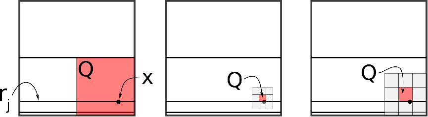
We begin by treating the case where x∈Ejx\in E_{j} for some 1≤j≤N1\leq j\leq N. Let Q∈𝒟Q\in\mathcal{D} be a dyadic square containing xx. The three essential cases of the proof are illustrated in Figure 1.

Refer to caption
Figure 1. The three cases: ℓ⁡(Q)>rj\ell(Q)>r_{j}, ℓ⁡(Q)<rj\ell(Q)<r_{j}, or ℓ⁡(Q)=rj\ell(Q)=r_{j}.

Suppose first that rj<ℓ⁡(Q)≤c0​r0r_{j}<\ell(Q)\leq c_{0}r_{0} for some absolute constant c0>0c_{0}>0 (c0=1/10c_{0}=1/10 is more than good enough). It follows that the lower edge JQJ_{Q} of QQ has to be contained in H=[0,r0]×{0}H=[0,r_{0}]\times\{0\}, since the second coordinate of xx is rj<ℓ⁡(Q)r_{j}<\ell(Q), and so JQ⊂ℝ×{0}J_{Q}\subset\mathbb{R}\times\{0\}. Since moreover ℓ⁡(Q)≤r0\ell(Q)\leq r_{0} and r0r_{0} is a dyadic number, we have that Q⊂[0,r0)2Q\subset[0,r_{0})^{2}, and so JQ⊂HJ_{Q}\subset H. Using this,

(2.2) μ⁡(3​Q)≥μ⁡(Q)≥μ⁡(Q∩H)=Θ⋅ℋ1​(JQ)=Θ⋅ℓ⁡(Q)=ϵ​ℓ​(Q)r0.\mu(3Q)\geq\mu(Q)\geq\mu(Q\cap H)=\Theta\cdot\mathcal{H}^{1}(J_{Q})=\Theta\cdot\ell(Q)=\frac{\epsilon\ell(Q)}{r_{0}}.

We, temporarily, further assume that rj<ℓ⁡(Q)≤c0​rj−1r_{j}<\ell(Q)\leq c_{0}r_{j-1}; this implies that 3​Q3Q does not meet the segment Ej−1E_{j-1} (for c0>0c_{0}>0 small enough), and hence by testing the β\beta-numbers with the line L=ℝ×{0}L=\mathbb{R}\times\{0\} we get the following estimate:

∑rj<ℓ⁡(Q)≤c0​rj−1β2,μ2​(3​Q)​ℓ⁡(Q)μ⁡(Q)​1Q​(x)\displaystyle\sum_{r_{j}<\ell(Q)\leq c_{0}r_{j-1}}\beta^{2}_{2,\mu}(3Q)\frac{\ell(Q)}{\mu(Q)}1_{Q}(x) ≲∑rj<ℓ⁡(Q)≤c0​rj−11Q​(x)​r02ϵ​ℓ​(Q)​∑i=1N∫3​Q∩Ei(riℓ⁡(Q))2​d​ℋ1\displaystyle\lesssim\sum_{r_{j}<\ell(Q)\leq c_{0}r_{j-1}}\frac{1_{Q}(x)r_{0}^{2}}{\epsilon\ell(Q)}\sum_{i=1}^{N}\int_{3Q\cap E_{i}}\left(\frac{r_{i}}{\ell(Q)}\right)^{2}\,d\mathcal{H}^{1}
≲∑rj<ℓ⁡(Q)≤c0​rj−11Q​(x)​r02ϵ​ℓ​(Q)2​∑i=jNri2∼r02ϵ.\displaystyle\lesssim\sum_{r_{j}<\ell(Q)\leq c_{0}r_{j-1}}1_{Q}(x)\frac{r_{0}^{2}}{\epsilon\ell(Q)^{2}}\sum_{i=j}^{N}r_{i}^{2}\sim\frac{r_{0}^{2}}{\epsilon}.

The same estimate also holds, if one sums over cubes QQ such that x∈Qx\in Q and c0​ri≤ℓ⁡(Q)≤c0​ri−1c_{0}r_{i}\leq\ell(Q)\leq c_{0}r_{i-1} for any 1≤i≤j−11\leq i\leq j-1 (note also that ℓ⁡(Q)>rj\ell(Q)>r_{j} in this case if the sequence (rj)(r_{j}) decays rapidly enough, which guarantees that we have the lower bound for μ⁡(Q)\mu(Q) exactly as above). There are at most N≤1/(ϵ​r0)N\leq 1/(\epsilon r_{0}) such indices ii, so it follows that

∑rj<ℓ⁡(Q)≤c0​r0β2,μ2​(3​Q)​ℓ⁡(Q)μ⁡(Q)​1Q​(x)≲r0ϵ2=c​ϵ.\sum_{r_{j}<\ell(Q)\leq c_{0}r_{0}}\beta^{2}_{2,\mu}(3Q)\frac{\ell(Q)}{\mu(Q)}1_{Q}(x)\lesssim\frac{r_{0}}{\epsilon^{2}}=c\epsilon.

This completes the case rj<ℓ⁡(Q)≤c0​r0r_{j}<\ell(Q)\leq c_{0}r_{0}.

If ℓ⁡(Q)≤rj\ell(Q)\leq r_{j}, then the lower edge of QQ is contained in EjE_{j}. In the case of strict inequality ℓ⁡(Q)<rj\ell(Q)<r_{j}, we have ℓ⁡(Q)≤rj/2\ell(Q)\leq r_{j}/2, and so 3​Q3Q intersects no line segments besides EjE_{j} (if the sequence (rj)(r_{j}) decays rapidly enough). It follows that β2,μ2​(3​Q)=0\beta^{2}_{2,\mu}(3Q)=0 in case ℓ⁡(Q)<rj\ell(Q)<r_{j}, and there is nothing to prove.

Finally, if ℓ⁡(Q)=rj\ell(Q)=r_{j}, then 3​Q3Q just intersects HH, and in fact ℋ1​(3​Q∩H)∼ℓ⁡(Q)\mathcal{H}^{1}(3Q\cap H)\sim\ell(Q). It follows that

μ⁡(3​Q)≳ϵ​ℓ​(Q)r0.\mu(3Q)\gtrsim\frac{\epsilon\ell(Q)}{r_{0}}.

For μ⁡(Q)\mu(Q) we get a worse estimate, because QQ does not meet HH:

μ⁡(Q)≥ϵ​ℋ1​(Ej∩Q)=ϵ​ℓ​(Q).\mu(Q)\geq\epsilon\mathcal{H}^{1}(E_{j}\cap Q)=\epsilon\ell(Q).

Assuming that the decay of the numbers (ri)(r_{i}) is rapid enough, the square 3​Q3Q does not meet the line segments EiE_{i} for i≤j−1i\leq j-1, so we get the following estimate for the number β2,μ2​(3​Q)\beta^{2}_{2,\mu}(3Q) (using L=ℝ×{0}L=\mathbb{R}\times\{0\} as the testing line):

β2,μ2​(3​Q)≲r0ℓ⁡(Q)​∑i=1N∫3​Q∩Ei(riℓ⁡(Q))2​d​ℋ1≲r0ℓ​(Q)2​∑i=jNri2≲r0.\beta^{2}_{2,\mu}(3Q)\lesssim\frac{r_{0}}{\ell(Q)}\sum_{i=1}^{N}\int_{3Q\cap E_{i}}\left(\frac{r_{i}}{\ell(Q)}\right)^{2}\,d\mathcal{H}^{1}\lesssim\frac{r_{0}}{\ell(Q)^{2}}\sum_{i=j}^{N}r_{i}^{2}\lesssim r_{0}.

Consequently,

∑ℓ⁡(Q)=rjβ2,μ2​(3​Q)​ℓ⁡(Q)μ⁡(Q)​1Q​(x)≲r0ϵ=c​ϵ2.\sum_{\ell(Q)=r_{j}}\beta^{2}_{2,\mu}(3Q)\frac{\ell(Q)}{\mu(Q)}1_{Q}(x)\lesssim\frac{r_{0}}{\epsilon}=c\epsilon^{2}.

This completes the proof in the case x∈Ejx\in E_{j}, except for the squares QQ with ℓ⁡(Q)≥c0​r0\ell(Q)\geq c_{0}r_{0}. In that case, the lower edge of QQ is again contained on ℝ×{0}\mathbb{R}\times\{0\}, and μ⁡(Q)∼1∼μ⁡(3​Q)\mu(Q)\sim 1\sim\mu(3Q). Thus,

β2,μ2​(3​Q)≲ϵ​∑i=1N∫Ei(riℓ⁡(Q))2​d​ℋ1≲ϵ​r03ℓ​(Q)2,\beta^{2}_{2,\mu}(3Q)\lesssim\epsilon\sum_{i=1}^{N}\int_{E_{i}}\left(\frac{r_{i}}{\ell(Q)}\right)^{2}\,d\mathcal{H}^{1}\lesssim\frac{\epsilon r_{0}^{3}}{\ell(Q)^{2}},

and so

∑ℓ⁡(Q)≥c0​r0β2,μ2​(3​Q)​ℓ⁡(Q)μ⁡(Q)​1Q​(x)≲ϵ​r03​∑ℓ⁡(Q)≥c0​r01Q​(x)ℓ⁡(Q)∼ϵ​r02=c2​ϵ7.\sum_{\ell(Q)\geq c_{0}r_{0}}\beta_{2,\mu}^{2}(3Q)\frac{\ell(Q)}{\mu(Q)}1_{Q}(x)\lesssim\epsilon r_{0}^{3}\sum_{\ell(Q)\geq c_{0}r_{0}}\frac{1_{Q}(x)}{\ell(Q)}\sim\epsilon r_{0}^{2}=c^{2}\epsilon^{7}.

It remains to consider the case x∈Hx\in H. If Q∋xQ\ni x is a dyadic square of side-length ℓ⁡(Q)≤c0​r0\ell(Q)\leq c_{0}r_{0}, then the lower edge of QQ is obviously contained in HH, and we have the estimates (2.2) for μ⁡(Q)\mu(Q) and μ⁡(3​Q)\mu(3Q). This allows us to make the same computations as in the case ℓ⁡(Q)>rj\ell(Q)>r_{j} above, and the β\beta-sum is again bounded by ≲r0/ϵ2=c​ϵ\lesssim r_{0}/\epsilon^{2}=c\epsilon. The case ℓ⁡(Q)≥c0​r0\ell(Q)\geq c_{0}r_{0} is exactly the same as above. The proof of Theorem 1.3 is complete.

Remark 2.3.

For our examples, and for the theory in whole, it is irrelevant whether the dyadic squares in 𝒟\mathcal{D} are taken to be half-open or closed. Only minor modifications are required in the arguments.

3. Proof of Theorem 1.2

We define the measure μ\mu as a weak limit of certain measures μn\mu_{n}. Assume that ϵ∈(0,2−10)\epsilon\in(0,2^{-10}) is a dyadic number, and set

μ1:=ν⁡((r1,j),1,ϵ),\mu_{1}:=\nu((r_{1,j}),1,\epsilon),

where (r1,j)j=0N1(r_{1,j})_{j=0}^{N_{1}} is a suitable sequence of dyadic radii to be specified later, with

r1,0=c​ϵ10andN1=12​ϵ​r1,0r_{1,0}=c\epsilon^{10}\quad\text{and}\quad N_{1}=\frac{1}{2\epsilon r_{1,0}}

for some small constant c>0c>0. Then N1​ϵ​r1,0=1/2≤1N_{1}\epsilon r_{1,0}=1/2\leq 1, so the upper bound condition for NN from Definition 2.1 is satisfied. Next, assume that the probability measure μn\mu_{n} has already been defined for some n≥1n\geq 1, and μn\mu_{n} has the form

μn=∑i∈Inωin⋅ℋ1|Jin,\mu_{n}=\sum_{i\in I_{n}}\omega_{i}^{n}\cdot\mathcal{H}^{1}|_{J_{i}^{n}},

where the numbers ωin\omega_{i}^{n} are positive dyadic numbers, and the sets JinJ_{i}^{n} are line segments of the form Jin=[ain,bin]×{cin}J_{i}^{n}=[a^{n}_{i},b^{n}_{i}]\times\{c^{n}_{i}\}, where ain,bin,cina^{n}_{i},b^{n}_{i},c^{n}_{i} are dyadic rationals. Further, assume that bin−ain=dnb^{n}_{i}-a^{n}_{i}=d_{n} is a positive dyadic rational depending only on nn.

To define μn+1\mu_{n+1}, choose an equally spaced set of dyadic rationals from the interval [0,dn][0,d_{n}], with "spacing" σn>0\sigma_{n}>0, and call this set DnD_{n}. More precisely,

Dn={0,σn,…,dn−σn},D_{n}=\{0,\sigma_{n},\ldots,d_{n}-\sigma_{n}\},

so that |Dn|=dn/σn|D_{n}|=d_{n}/\sigma_{n}.

The size of the number σn\sigma_{n} is determined by the mutual distances between distinct line segments JinJ_{i}^{n}. In fact, if the minimal distance between any distinct pair of line segments Ji1n,Ji2nJ_{i_{1}}^{n},J_{i_{2}}^{n} is Δn\Delta_{n}, then we set

(3.1) σn:=Δn1000.\sigma_{n}:=\frac{\Delta_{n}}{1000}.

Next, for a fixed segment JinJ_{i}^{n} with i∈Ini\in I_{n}, write

(3.2) mni:=ωin​dn|Dn|=σn​ωin.m_{n}^{i}:=\frac{\omega_{i}^{n}d_{n}}{|D_{n}|}=\sigma_{n}\omega_{i}^{n}.

Then, pick a decreasing sequence of dyadic radii (rn+1,j)j=0Nn+1i(r_{n+1,j})_{j=0}^{N^{i}_{n+1}}, where

(3.3) Nn+1i=2n−1​minϵ​rn+1,0,N^{i}_{n+1}=\frac{2^{n-1}m^{n}_{i}}{\epsilon r_{n+1,0}},

and set

νn+1i:=ν⁡((rn+1,j)j=0Nn+1i,mni,ϵ/2n).\nu^{i}_{n+1}:=\nu((r_{n+1,j})_{j=0}^{N^{i}_{n+1}},m_{n}^{i},\epsilon/2^{n}).

Note that the choice of Nn+1iN_{n+1}^{i} is a dyadic positive integer, if rn+1,0r_{n+1,0} is a small enough dyadic number, where "small enough" only depends on the generation nn quantities mnim_{n}^{i}. Note that only the length of the sequence (rn+1,j)j=0Nn+1i(r_{n+1,j})^{N^{i}_{n+1}}_{j=0} depends on the index i∈Ini\in I_{n}, but the numbers themselves are all part of some single rapidly decreasing infinite sequence, which only depends on n+1n+1. We assume that

(3.4) rn+1,0≤min⁡{(ϵ​Δn)10100,(ϵ​m​(n))1022​n},r_{n+1,0}\leq\min\left\{\frac{(\epsilon\Delta_{n})^{10}}{100},\frac{(\epsilon m(n))^{10}}{2^{2n}}\right\},

where m⁡(n)=min⁡{mni:i∈In}m(n)=\min\{m^{i}_{n}:i\in I_{n}\}.

After the definition of νn+1i\nu_{n+1}^{i} has been made for every segment JinJ^{n}_{i}, we define the measure μn+1\mu_{n+1} as

μn+1:=∑i∈In∑t∈Dn[(ain+t,cin)+νn+1i].\mu_{n+1}:=\sum_{i\in I_{n}}\sum_{t\in D_{n}}[(a_{i}^{n}+t,c_{i}^{n})+\nu^{i}_{n+1}].

The notation (ain+t,cin)+vn+1i(a_{i}^{n}+t,c_{i}^{n})+v^{i}_{n+1} simply means the measure νn+1i\nu^{i}_{n+1} translated by the vector (ain+t,cin)(a_{i}^{n}+t,c_{i}^{n}). With this definition, μn+1\mu_{n+1} is a probability measure:

μn+1​(ℝ2)=∑i∈In∑t∈Dnωin​dn|Dn|=∑i∈Inωin​dn=μn​(ℝ2)=1.\mu_{n+1}(\mathbb{R}^{2})=\sum_{i\in I_{n}}\sum_{t\in D_{n}}\frac{\omega_{i}^{n}d_{n}}{|D_{n}|}=\sum_{i\in I_{n}}\omega_{i}^{n}d_{n}=\mu_{n}(\mathbb{R}^{2})=1.

For a given interval JinJ^{n}_{i}, i∈Ini\in I_{n}, the choice of Nn+1iN_{n+1}^{i} was made so that for every t∈Dnt\in D_{n} we have

[(ain+t,cin)+νn+1i]​(Jin)=min−Nn+1i⋅ϵ2n⋅rn+1,0=min2.\displaystyle[(a_{i}^{n}+t,c_{i}^{n})+\nu^{i}_{n+1}](J^{n}_{i})=m^{n}_{i}-N^{i}_{n+1}\cdot\frac{\epsilon}{2^{n}}\cdot r_{n+1,0}=\frac{m^{n}_{i}}{2}.

In particular, we have

(3.5) μn+1​(Jin)=∑t∈Dn[(ain+t,cin)+νn+1i]​(Jin)=|Dn|​min2=μn​(Jin)2.\mu_{n+1}(J^{n}_{i})=\sum_{t\in D_{n}}[(a_{i}^{n}+t,c_{i}^{n})+\nu^{i}_{n+1}](J^{n}_{i})=|D_{n}|\frac{m^{n}_{i}}{2}=\frac{\mu_{n}(J^{n}_{i})}{2}.

If the numbers rn,0r_{n,0} converge to zero quickly enough as n→∞n\to\infty, one can check that the measures μn\mu_{n} converge weakly to a limit probability measure on [0,1]2[0,1]^{2}, which is our final measure μ\mu.

Before proving (i) and (ii), we make a few useful remarks about the structure of μ\mu and its support. First, the support of each measure μn+1\mu_{n+1} is contained in a finite union of closures of dyadic squares of side-length rn+1,0r_{n+1,0}, namely

𝒬~n+1={(ain+t,cin)+[0,rn+1,0]2:i∈In,t∈Dn},\tilde{\mathcal{Q}}_{n+1}=\{(a_{i}^{n}+t,c_{i}^{n})+[0,r_{n+1,0}]^{2}:i\in I_{n},t\in D_{n}\},

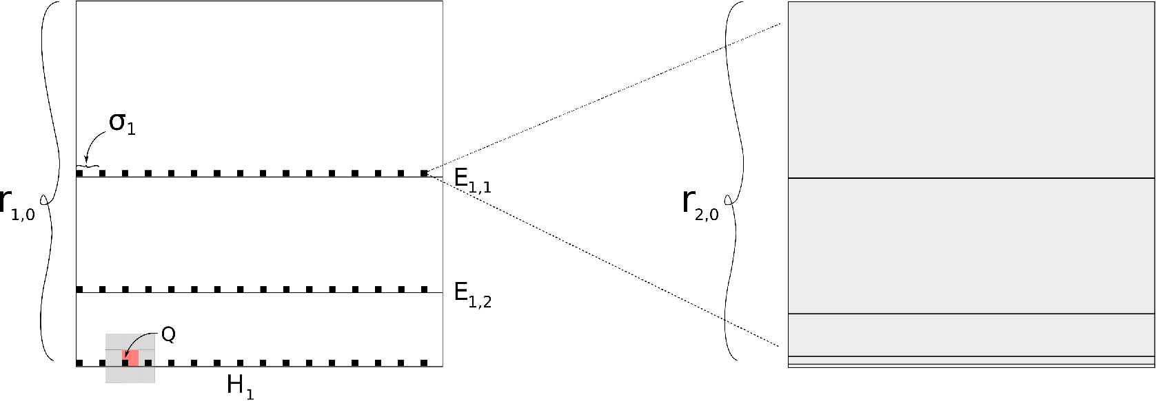
see Figure 2. The same is true for the measure μ\mu, and in fact we even have the improved conclusion that the support of μ\mu is contained in the union of the proper dyadic squares

𝒬n+1={(ain+t,cin)+[0,rn+1,0)2:i∈In,t∈Dn}.\mathcal{Q}_{n+1}=\{(a_{i}^{n}+t,c_{i}^{n})+[0,r_{n+1,0})^{2}:i\in I_{n},t\in D_{n}\}.

This improvement is due to the fact that the squares in 𝒬n+2\mathcal{Q}_{n+2} contained in a square Q∈𝒬n+1Q\in\mathcal{Q}_{n+1} always stay at positive distance from the two "open sides" of the dyadic square QQ.

The following observation is an immediate corollary of the previous discussion, and the fact that for a fixed segment JinJ_{i}^{n}, the squares (ain+t,cin)+[0,rn+1,0]2(a_{i}^{n}+t,c_{i}^{n})+[0,r_{n+1,0}]^{2} lie in a single row "on top" of JinJ_{i}^{n}:

Lemma 3.6.

If n≥1n\geq 1 and JinJ_{i}^{n}, i∈Ini\in I_{n}, are the segments appearing in the definition of μn\mu_{n}, then spt⁡μ\operatorname{spt}\mu is contained in the union of rectangles of the form

Rin=⋃h∈[0,rn+1,0][Jin+(0,h)],R^{n}_{i}=\bigcup_{h\in[0,r_{n+1,0}]}[J^{n}_{i}+(0,h)],

and μ⁡(Rin)=μn​(Jin)\mu(R^{n}_{i})=\mu_{n}(J^{n}_{i}).

Refer to caption
Figure 2. The squares in 𝒬2\mathcal{Q}_{2}, and the small square QQ appearing in the proof of Lemma 3.9. The grey area around QQ is 3​Q3Q.

Since the side-lengths rn+1,0r_{n+1,0} are, by (3.4), far smaller than both the "spacing" σn\sigma_{n} and the distance Δn\Delta_{n}, the following holds for all squares Q1,Q2∈𝒬n+1Q_{1},Q_{2}\in\mathcal{Q}_{n+1}:

(3.7) d⁡(Q1,Q2)≥5​rn+1,0.d(Q_{1},Q_{2})\geq 5r_{n+1,0}.

This gives the following observation:

Lemma 3.8.

For every point x∈spt⁡μx\in\operatorname{spt}\mu there exists a unique sequence of dyadic squares Q1,Q2,…Q_{1},Q_{2},\ldots with

Qn∈𝒬nandx∈Qn.Q_{n}\in\mathcal{Q}_{n}\quad\text{and}\quad x\in Q_{n}.

The square QnQ_{n} in this sequence will be denoted by Qn​(x)Q_{n}(x).

Observe that to every square Q∈𝒬n+1Q\in\mathcal{Q}_{n+1}, n≥0n\geq 0, one may canonically associate a sequence

(rn+1,j)j=0Nn+1Q(r_{n+1,j})_{j=0}^{N^{Q}_{n+1}}

and a measure νQ\nu_{Q}. For example, for n=0n=0, the collection 𝒬n+1=𝒬1\mathcal{Q}_{n+1}=\mathcal{Q}_{1} consists of the single square [0,r1,0)2[0,r_{1,0})^{2}, so the sequence is (r1,j)j=0N1(r_{1,j})_{j=0}^{N_{1}} and the measure is νQ=μ1\nu_{Q}=\mu_{1}. In general, the measure νQ\nu_{Q} is simply νQ=μn+1|Q\nu_{Q}=\mu_{n+1}|_{Q}. Then

νQ=(ain+t,cin)+νn+1i\nu_{Q}=(a_{i}^{n}+t,c_{i}^{n})+\nu^{i}_{n+1}

for some i∈Ini\in I_{n} and t∈Dnt\in D_{n}, and the "canonical sequence" (rn+1,j)(r_{n+1,j}) associated to QQ is

(rn+1,j)n=0Nn+1Q:=(rn+1,j)j=0Nn+1i(r_{n+1,j})_{n=0}^{N^{Q}_{n+1}}:=(r_{n+1,j})_{j=0}^{N^{i}_{n+1}}

for this particular ii. With this notation in mind, we prove another lemma:

Lemma 3.9.

Suppose n≥1n\geq 1, and QQ is a dyadic square containing a point x∈spt⁡μx\in\operatorname{spt}\mu. Let Qn=Qn​(x)∈𝒬nQ_{n}=Q_{n}(x)\in\mathcal{Q}_{n} be the square defined in Lemma 3.8. Let (rn,j)(r_{n,j}), 0≤j≤NnQn=:N0\leq j\leq N^{Q_{n}}_{n}=:N be the sequence define above, and assume that

ℓ⁡(Q)<rn,N/2.\ell(Q)<r_{n,N}/2.

Then, all the squares Q′∈𝒬n+1Q^{\prime}\in\mathcal{Q}_{n+1} with 3​Q∩Q′≠∅3Q\cap Q^{\prime}\neq\emptyset are horizontal translates of each other, and in fact the measures μn+1|Q′\mu_{n+1}|_{Q^{\prime}} for such Q′Q^{\prime} are horizontal translates of each other.

Proof.

A possible position of the square QQ is depicted in the left half of Figure 2. We only prove the lemma in the case n=1n=1; the general case is no different but would require introducing even more notation. In the case n=1n=1, the index set In=I1I_{n}=I_{1} is {1,…,N1,N1+1}\{1,\ldots,N_{1},N_{1}+1\}, and the segments Ji1J^{1}_{i} are the segments E1,jE_{1,j} (for 1≤j≤N11\leq j\leq N_{1}) and JN1+11=H1J^{1}_{N_{1}+1}=H_{1}. Further, N=N1N=N_{1}.

The main assumption ℓ⁡(Q)<r1,N1/2\ell(Q)<r_{1,N_{1}}/2 means that the side-length of QQ is less than half of the minimal (vertical) gap between the segments E1,jE_{1,j} and H1H_{1} – indeed this minimal gap is the one between E1,N1=[0,r1,0]×{r1,N1}E_{1,N_{1}}=[0,r_{1,0}]\times\{r_{1,N_{1}}\} and H1=[0,r1,0]×{0}H_{1}=[0,r_{1,0}]\times\{0\}. Since QQ is a dyadic square, and the numbers r1,jr_{1,j} are all dyadic, this implies that QQ is entirely contained in some slab of the form ℝ×[a,b)\mathbb{R}\times[a,b), where a<ba<b and a,ba,b are consecutive elements from {0,r1,N1,…,r1,1,∞}\{0,r_{1,N_{1}},\ldots,r_{1,1},\infty\}. Assume, for example, that

Q⊂ℝ×[0,r1,N1),Q\subset\mathbb{R}\times[0,r_{1,N_{1}}),

as in Figure 2. The other cases are handled similarly. Since Q∩spt⁡μ≠∅Q\cap\operatorname{spt}\mu\neq\emptyset, and spt⁡μ\operatorname{spt}\mu is contained in the union of the squares 𝒬2\mathcal{Q}_{2}, we conclude that either QQ is contained in one of the squares in 𝒬2\mathcal{Q}_{2} (if ℓ⁡(Q)≤r2,0\ell(Q)\leq r_{2,0}) and the lemma is trivial, or else (if ℓ⁡(Q)>r2,0\ell(Q)>r_{2,0}), QQ contain a square Q′∈𝒬2Q^{\prime}\in\mathcal{Q}_{2} with Q′⊂ℝ×[0,r1,N1)Q^{\prime}\subset\mathbb{R}\times[0,r_{1,N_{1}}). Such a square Q′Q^{\prime} must have an edge contained in ℝ×{0}\mathbb{R}\times\{0\}, so also QQ has an edge contained in ℝ×{0}\mathbb{R}\times\{0\}. Since ℓ⁡(Q)<r1,N1/2\ell(Q)<r_{1,N_{1}}/2, it follows that the yy-coordinate of every point in 3​Q3Q is strictly smaller than r1,N1r_{1,N_{1}}. Thus, 3​Q3Q does not meet any of the rectangles Ri1R_{i}^{1} for 1≤i≤N11\leq i\leq N_{1}. On the other hand, the squares Q′∈𝒬2Q^{\prime}\in\mathcal{Q}_{2} contained in RN1+11R^{1}_{N_{1}+1} are, indeed, horizontal translates of each other (inspecting the definition of 𝒬2\mathcal{Q}_{2}, they have the form Q′=(t,0)+[0,r2,1)2Q^{\prime}=(t,0)+[0,r_{2,1})^{2}, t∈D1t\in D_{1}). The same is true about the measures: in this particular case they all have the form

(t,0)+ν⁡((r2,j)j=0N2N1+1,m1N1+1,ϵ/2),t∈D1.(t,0)+\nu((r_{2,j})_{j=0}^{N^{N_{1}+1}_{2}},m_{1}^{N_{1}+1},\epsilon/2),\quad t\in D_{1}.

This completes the proof. ∎

3.1. Lower density vanishes

We say that a generation nn, n≥1n\geq 1, segment JinJ^{n}_{i}, i∈Ini\in I_{n}, is of type EE, if it is not the lower edge of a square in 𝒬n\mathcal{Q}_{n}. The lower edges of squares in 𝒬n\mathcal{Q}_{n} are called type HH. Let n≥1n\geq 1 and k≥0k\geq 0. Suppose that JinJ^{n}_{i} is of type EE and that x∈Rinx\in R^{n}_{i} (recall the notation from Lemma 3.6).

We define Nn=max⁡NniN_{n}=\max N_{n}^{i}. If k=0k=0 we clearly have by construction that

μn​(B⁡(x,rn,Nn/2))≤ϵ2n−1​rn,Nn.\mu_{n}(B(x,r_{n,N_{n}}/2))\leq\frac{\epsilon}{2^{n-1}}r_{n,N_{n}}.

Suppose then that k=1k=1. The ball B⁡(x,rn,Nn/2)B(x,r_{n,N_{n}}/2) can intersect at most rn,Nn/σnr_{n,N_{n}}/\sigma_{n} squares in 𝒬n+1\mathcal{Q}_{n+1}. Therefore, we have

μn+1​(B⁡(x,rn,Nn/2))≤rn,Nnσn​ϵ2n−1​rn,0|Dn|=ϵ2n−1​rn,Nn.\mu_{n+1}(B(x,r_{n,N_{n}}/2))\leq\frac{r_{n,N_{n}}}{\sigma_{n}}\frac{\frac{\epsilon}{2^{n-1}}r_{n,0}}{|D_{n}|}=\frac{\epsilon}{2^{n-1}}r_{n,N_{n}}.

The same proof yields with all k≥0k\geq 0 that

μn+k​(B⁡(x,rn,Nn/2))≤ϵ2n−1​rn,Nn.\mu_{n+k}(B(x,r_{n,N_{n}}/2))\leq\frac{\epsilon}{2^{n-1}}r_{n,N_{n}}.

Letting k→∞k\to\infty we get (recall that μ⁡(G)≤lim infm→∞μm​(G)\mu(G)\leq\liminf_{m\to\infty}\mu_{m}(G) for open sets GG):

μ⁡(B⁡(x,rn,Nn/2))≤ϵ2n−1​rn,Nn.\mu(B(x,r_{n,N_{n}}/2))\leq\frac{\epsilon}{2^{n-1}}r_{n,N_{n}}.

We can conclude that

Θ∗1​(μ,x)=0,\Theta_{*}^{1}(\mu,x)=0,

if xx belongs to infinitely many RinR^{n}_{i}, where the corresponding intervals JinJ^{n}_{i} are of type EE.

Next, let us prove that μ⁡(Jin)=0\mu(J^{n}_{i})=0 for all n≥1n\geq 1 and i∈Ini\in I_{n}. Indeed, notice that for every k≥1k\geq 1 we have

μ⁡(Jin)\displaystyle\mu(J^{n}_{i}) ≤μ⁡(⋃h∈[0,rn+k,Nn+k)[Jin+(0,h)])\displaystyle\leq\mu\Bigg(\bigcup_{h\in[0,r_{n+k,N_{n+k}})}[J^{n}_{i}+(0,h)]\Bigg)
=μn+k​(⋃h∈[0,rn+k,Nn+k)[Jin+(0,h)])=μn+k​(Jin)≤μn​(Jin)2k≤2−k.\displaystyle=\mu_{n+k}\Bigg(\bigcup_{h\in[0,r_{n+k,N_{n+k}})}[J^{n}_{i}+(0,h)]\Bigg)=\mu_{n+k}(J^{n}_{i})\leq\frac{\mu_{n}(J^{n}_{i})}{2^{k}}\leq 2^{-k}.

Here we used how the measures are constructed and (3.5).

Define

A=⋃n0≥1⋂n≥n0{x∈sptμ:x∈Rin, where Jin is of type H}.A=\bigcup_{n_{0}\geq 1}\bigcap_{n\geq n_{0}}\{x\in\operatorname{spt}\mu\colon\,x\in R^{n}_{i},\textup{ where }J^{n}_{i}\textup{ is of type }H\}.

To conclude that Θ∗1​(μ,x)=0\Theta_{*}^{1}(\mu,x)=0 for μ\mu-a.e. xx, it is enough to prove that μ⁡(A)=0\mu(A)=0. This follows from the inclusion

A⊂⋃n≥1⋃i∈InJin,A\subset\bigcup_{n\geq 1}\bigcup_{i\in I_{n}}J_{i}^{n},

and the fact that μ⁡(Jin)=0\mu(J_{i}^{n})=0 for all n,in,i.

3.2. The estimate for Jones’ square function

In this subsection, we prove that

(3.10) ∑Q∈𝒟β2,μ2​(3​Q)​ℓ⁡(Q)μ⁡(Q)​ 1Q​(x)≲ϵ,x∈spt⁡μ,\sum_{Q\in\mathcal{D}}\beta^{2}_{2,\mu}(3Q)\frac{\ell(Q)}{\mu(Q)}\,1_{Q}(x)\lesssim\epsilon,\quad x\in\operatorname{spt}\mu,

if the parameters in the construction of μ\mu are chosen appropriately. Fix x∈spt⁡μx\in\operatorname{spt}\mu, and let Qn:=Qn​(x)Q_{n}:=Q_{n}(x) be the squares defined in Lemma 3.8. As explained above Lemma 3.9, the square sequence (Qn)n=1∞(Q_{n})_{n=1}^{\infty} gives rise to a sequence of numbers Nn:=NnQnN_{n}:=N_{n}^{Q_{n}}, n≥1n\geq 1, and associated sequence of sequences

(rn,j)j=0Nn=(rn,j)j=0NnQn,n≥1.(r_{n,j})_{j=0}^{N_{n}}=(r_{n,j})_{j=0}^{N^{Q_{n}}_{n}},\quad n\geq 1.

Heuristically, these sequences tell us, what kind of "pictures" we see as we zoom to xx along the rapidly shrinking dyadic squares QnQ_{n}. The challenge of the proof below will be to handle the β\beta-numbers for dyadic squares Q∋xQ\ni x, whose side-length lies (far) between the side-lengths of consecutive squares QnQ_{n} and Qn+1Q_{n+1}. More precisely, we aim to prove that

(3.11) ∑rn,Nn/2≤ℓ⁡(Q)<rn−1,Nn−1/2β2,μ2​(3​Q)​ℓ⁡(Q)μ⁡(Q)​ 1Q​(x)≲ϵ/2n\sum_{r_{n,N_{n}}/2\leq\ell(Q)<r_{n-1,N_{n-1}}/2}\beta^{2}_{2,\mu}(3Q)\frac{\ell(Q)}{\mu(Q)}\,1_{Q}(x)\lesssim\epsilon/2^{n}

for n≥1n\geq 1, where we agree that r0,N0=1r_{0,N_{0}}=1. This still leaves the sum over the squares with ℓ⁡(Q)≥1/2\ell(Q)\geq 1/2, but this is easy and will be treated at the end of the proof. The upper bound ℓ⁡(Q)<rn−1,Nn−1/2≤rn−1,0\ell(Q)<r_{n-1,N_{n-1}}/2\leq r_{n-1,0} guarantees (recalling the separation condition (3.7)) that every square appearing in the summation only meets one of the squares in 𝒬n−1\mathcal{Q}_{n-1}, namely Qn−1Q_{n-1}. Moreover, since ℓ⁡(Q)<rn−1,Nn−1/2\ell(Q)<r_{n-1,N_{n-1}}/2, Lemma 3.9 guarantees that the squares in

𝒬n​(3​Q):={Q′∈𝒬n:Q′∩3​Q≠∅},\mathcal{Q}_{n}(3Q):=\{Q^{\prime}\in\mathcal{Q}_{n}:Q^{\prime}\cap 3Q\neq\emptyset\},

are horizontal translates of each other, and the same is true for the measures μn|Q′\mu_{n}|_{Q^{\prime}} with Q′∈𝒬n​(3​Q)Q^{\prime}\in\mathcal{Q}_{n}(3Q). In particular, these measures have a common mass mm, and by construction, μ⁡(Q′)=μn​(Q′)=m\mu(Q^{\prime})=\mu_{n}(Q^{\prime})=m for all Q′∈𝒬n​(3​Q)Q^{\prime}\in\mathcal{Q}_{n}(3Q).

We first prove (3.11) for the dyadic squares QQ with ℓ⁡(Q)\ell(Q) in the restricted range

(3.12) rn,0≤ℓ⁡(Q)<rn−1,Nn−1/2.r_{n,0}\leq\ell(Q)<r_{n-1,N_{n-1}}/2.
Refer to caption
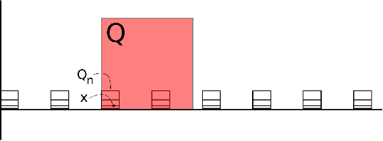
Figure 3. The case rn,0≤ℓ⁡(Q)<rn−1,Nn−1/2r_{n,0}\leq\ell(Q)<r_{n-1,N_{n-1}}/2.

This case is depicted in Figure 3. Since x∈Qx\in Q and ℓ⁡(Q)≥rn,0\ell(Q)\geq r_{n,0}, the square QQ contains the dyadic square of side-length rn,0r_{n,0} containing xx, namely QnQ_{n}. This gives μ⁡(Q)≥μ⁡(Qn)=m\mu(Q)\geq\mu(Q_{n})=m. If q:=card⁡𝒬n​(3​Q)q:=\operatorname{card}\mathcal{Q}_{n}(3Q), then in fact

(3.13) μ⁡(3​Q)≥μ⁡(Q)≳q​m,\mu(3Q)\geq\mu(Q)\gtrsim qm,

which follows easily from the inequality μ⁡(Q)≥m\mu(Q)\geq m, and the fact that the squares in 𝒬n​(3​Q)\mathcal{Q}_{n}(3Q) are horizontal translates of each other. In order to make further progress in estimating the number β2,μ2​(3​Q)\beta_{2,\mu}^{2}(3Q), we need to understand – and set up notation on – how μ\mu looks like inside the squares Q′∈𝒬n​(3​Q)Q^{\prime}\in\mathcal{Q}_{n}(3Q). By definition, μn\mu_{n} restricted to any square Q′∈𝒬n​(3​Q)Q^{\prime}\in\mathcal{Q}_{n}(3Q) has the form

μn|Q′=xQ′+ν⁡((rn,j)j=0Nn,m,ϵ/2n−1)=xQ′+∑j=1Nnϵ2n−1⋅ℋ1|En,j+Θn⋅ℋ1|Hn,\mu_{n}|_{Q^{\prime}}=x_{Q^{\prime}}+\nu((r_{n,j})^{N_{n}}_{j=0},m,\epsilon/2^{n-1})=x_{Q^{\prime}}+\sum_{j=1}^{N_{n}}\frac{\epsilon}{2^{n-1}}\cdot\mathcal{H}^{1}|_{E_{n,j}}+\Theta_{n}\cdot\mathcal{H}^{1}|_{H_{n}},

where xQ′x_{Q^{\prime}} is the lower left corner point of Q′Q^{\prime}, the En,jE_{n,j}’s and HnH_{n} are the line segments of length rn,0r_{n,0} defined in Definition 2.1, and Θn=Θn​(m)\Theta_{n}=\Theta_{n}(m) solves the equation

Nn​(ϵ/2n−1)​rn,0+Θn​rn,0=m.N_{n}(\epsilon/2^{n-1})r_{n,0}+\Theta_{n}r_{n,0}=m.

As pointed out in Lemma 3.6, the support of μ|Q′\mu|_{Q^{\prime}} lies close to the support of μn\mu_{n}: if

E~n,j:=⋃h∈[0,rn+1,0][En,j+(0,h)]\tilde{E}_{n,j}:=\bigcup_{h\in[0,r_{n+1,0}]}[E_{n,j}+(0,h)]

and similarly

H~n:=⋃h∈[0,rn+1,0][Hn+(0,h)],\tilde{H}_{n}:=\bigcup_{h\in[0,r_{n+1,0}]}[H_{n}+(0,h)],

then

spt⁡(μ|Q′)⊂xQ′+⋃j=1NnE~n,j∪H~n\operatorname{spt}(\mu|_{Q^{\prime}})\subset x_{Q^{\prime}}+\bigcup_{j=1}^{N_{n}}\tilde{E}_{n,j}\cup\tilde{H}_{n}

for Q′∈𝒬n​(3​Q)Q^{\prime}\in\mathcal{Q}_{n}(3Q). Recall that the measures μQ′\mu_{Q^{\prime}} with Q′∈𝒬n​(3​Q)Q^{\prime}\in\mathcal{Q}_{n}(3Q) are all horizontal translates of each other: this implies that, for each fixed 1≤j≤Nn1\leq j\leq N_{n}, the segments xQ′+En,jx_{Q^{\prime}}+E_{n,j} are contained on a single line LjL_{j}. Similarly, the segments xQ′+Hnx_{Q^{\prime}}+H_{n} are contained on a single line L=LNn+1L=L_{N_{n}+1}, and this line LL will be used to estimate the number β2,μ2​(3​Q)\beta_{2,\mu}^{2}(3Q). We use the following bounds:

d⁡(y,L)∼rn,j,y∈xQ′+E~n,j,d(y,L)\sim r_{n,j},\qquad y\in x_{Q^{\prime}}+\tilde{E}_{n,j},

and

d⁡(y,L)≤rn+1,0,y∈xQ′+H~n,d(y,L)\leq r_{n+1,0},\qquad y\in x_{Q^{\prime}}+\tilde{H}_{n},

for any Q′∈𝒬n​(3​Q)Q^{\prime}\in\mathcal{Q}_{n}(3Q). Consequently, recalling (3.13),

β2,μ2​(3​Q)\displaystyle\beta_{2,\mu}^{2}(3Q)
≲1q​m​∑Q′∈𝒬n​(3​Q)∫Q′(d⁡(y,L)ℓ⁡(Q))​𝑑μ​(y)\displaystyle\lesssim\frac{1}{qm}\sum_{Q^{\prime}\in\mathcal{Q}_{n}(3Q)}\int_{Q^{\prime}}\left(\frac{d(y,L)}{\ell(Q)}\right)\,d\mu(y)
≲1q​m​∑Q′∈𝒬n​(3​Q)[∫xQ′+H~n(rn+1,0ℓ⁡(Q))2​𝑑μ​(y)+∑j=1Nn∫xQ′+E~n,j(rn,jℓ⁡(Q))2​𝑑μ​(y)].\displaystyle\lesssim\frac{1}{qm}\sum_{Q^{\prime}\in\mathcal{Q}_{n}(3Q)}\left[\int_{x_{Q^{\prime}}+\tilde{H}_{n}}\left(\frac{r_{n+1,0}}{\ell(Q)}\right)^{2}\,d\mu(y)+\sum_{j=1}^{N_{n}}\int_{x_{Q^{\prime}}+\tilde{E}_{n,j}}\left(\frac{r_{n,j}}{\ell(Q)}\right)^{2}\,d\mu(y)\right].

We estimate the integrals separately. First, the trivial bound μ⁡(xQ′+H~n)≤m\mu(x_{Q^{\prime}}+\tilde{H}^{n})\leq m gives

∫xQ′+H~n(rn+1,0ℓ⁡(Q))2​𝑑μ​(y)≤m​(rn+1,0ℓ⁡(Q))2.\int_{x_{Q^{\prime}}+\tilde{H}_{n}}\left(\frac{r_{n+1,0}}{\ell(Q)}\right)^{2}\,d\mu(y)\leq m\left(\frac{r_{n+1,0}}{\ell(Q)}\right)^{2}.

For 1≤j≤Nn1\leq j\leq N_{n} we have μ⁡(xQ′+E~n,j)=μn​(xQ′+En,j)≤ℓ⁡(Q′)=rn,0\mu(x_{Q^{\prime}}+\tilde{E}_{n,j})=\mu_{n}(x_{Q^{\prime}}+E_{n,j})\leq\ell(Q^{\prime})=r_{n,0}, so that

∑j=1Nn∫xQ′+E~jn(rn,jℓ⁡(Q))2​𝑑μ​(y)≤rn,0ℓ​(Q)2​∑j=1Nnrn,j2≲rn,03ℓ​(Q)2.\sum_{j=1}^{N_{n}}\int_{x_{Q^{\prime}}+\tilde{E}_{j}^{n}}\left(\frac{r_{n,j}}{\ell(Q)}\right)^{2}\,d\mu(y)\leq\frac{r_{n,0}}{\ell(Q)^{2}}\sum_{j=1}^{N_{n}}r_{n,j}^{2}\lesssim\frac{r_{n,0}^{3}}{\ell(Q)^{2}}.

Altogether,

β2,μ2​(3​Q)≲(rn+1,0ℓ⁡(Q))2+1m​rn,03ℓ​(Q)2,\beta_{2,\mu}^{2}(3Q)\lesssim\left(\frac{r_{n+1,0}}{\ell(Q)}\right)^{2}+\frac{1}{m}\frac{r_{n,0}^{3}}{\ell(Q)^{2}},

so

∑rn,0≤ℓ⁡(Q)<rn−1,Nn−1/2\displaystyle\sum_{r_{n,0}\leq\ell(Q)<r_{n-1,N_{n-1}}/2} β2,μ2​(3​Q)​ℓ⁡(Q)μ⁡(Q)​1Q​(x)\displaystyle\beta^{2}_{2,\mu}(3Q)\frac{\ell(Q)}{\mu(Q)}1_{Q}(x)
≲∑rn,0≤ℓ⁡(Q)<rn−1,Nn−1/2[rn+1,02m⋅ℓ⁡(Q)+rn,03m2⋅ℓ⁡(Q)]​1Q​(x)\displaystyle\lesssim\sum_{r_{n,0}\leq\ell(Q)<r_{n-1,N_{n-1}}/2}\left[\frac{r_{n+1,0}^{2}}{m\cdot\ell(Q)}+\frac{r_{n,0}^{3}}{m^{2}\cdot\ell(Q)}\right]1_{Q}(x)
≲rn+1,02m⋅rn,0+rn,02m2≤rn+1,02m⁡(n−1)⋅rn,0+rn,02m​(n−1)2.\displaystyle\lesssim\frac{r_{n+1,0}^{2}}{m\cdot r_{n,0}}+\frac{r_{n,0}^{2}}{m^{2}}\leq\frac{r_{n+1,0}^{2}}{m(n-1)\cdot r_{n,0}}+\frac{r_{n,0}^{2}}{m(n-1)^{2}}.

Recalling the size condition (3.4) for rn,0r_{n,0} (the definition of m⁡(n−1)m(n-1) can also be found under (3.4)), the right hand side is certainly ≲ϵ/2n\lesssim\epsilon/2^{n}, as required by (3.11).

The next goal is to prove that

(3.14) ∑rn,Nn/2≤ℓ⁡(Q)<rn,0β2,μ2​(3​Q)​ℓ⁡(Q)μ⁡(Q)​ 1Q​(x)≲ϵ2n.\sum_{r_{n,N_{n}}/2\leq\ell(Q)<r_{n,0}}\beta^{2}_{2,\mu}(3Q)\frac{\ell(Q)}{\mu(Q)}\,1_{Q}(x)\lesssim\frac{\epsilon}{2^{n}}.

In this case, since ℓ⁡(Q)<rn,0\ell(Q)<r_{n,0} and the relevant squares QQ contain the point x∈Qn∈𝒬nx\in Q_{n}\in\mathcal{Q}_{n}, we have in fact Q⊂QnQ\subset Q_{n}, and also 3​Q3Q meets no other squares in 𝒬n\mathcal{Q}_{n} besides QnQ_{n}. To simplify notation, we assume that

Qn=[0,rn,0)2.Q_{n}=[0,r_{n,0})^{2}.

This has the benefit that the generation nn segments Ej=En,jE_{j}=E_{n,j} and H=HnH=H_{n} inside QnQ_{n} have the following simple expressions:

Ej=[0,rn,0]×{rn,j}andH=[0,rn,0]×{0}.E_{j}=[0,r_{n,0}]\times\{r_{n,j}\}\quad\text{and}\quad H=[0,r_{n,0}]\times\{0\}.

With this notation, recall that

μn|Qn=ν⁡((rn,j)j=0Nn,m,ϵ/2n−1)=∑j=1Nnϵ2n−1⋅ℋ1|Ej+Θ⋅ℋ1|H,\mu_{n}|_{Q_{n}}=\nu((r_{n,j})_{j=0}^{N_{n}},m,\epsilon/2^{n-1})=\sum_{j=1}^{N_{n}}\frac{\epsilon}{2^{n-1}}\cdot\mathcal{H}^{1}|_{E_{j}}+\Theta\cdot\mathcal{H}^{1}|_{H},

where Θ=Θn​(m)\Theta=\Theta_{n}(m) solves the equation

Nn​(ϵ/2n−1)​rn,0+Θ​rn,0=m.N_{n}(\epsilon/2^{n-1})r_{n,0}+\Theta r_{n,0}=m.

Recall from (3.3) and (3.2) that the number NnN_{n} satisfies

Nn=2n−2​mϵ​rn,0,N_{n}=\frac{2^{n-2}m}{\epsilon r_{n,0}},

so that

Θ=m2​rn,0∼mrn,0.\Theta=\frac{m}{2r_{n,0}}\sim\frac{m}{r_{n,0}}.

We also re-introduce the notation for the rectangles

E~j:=⋃h∈[0,rn+1,0][Ej+(0,h)]andH~:=⋃h∈[0,rn+1,0][H+(0,h)],\tilde{E}_{j}:=\bigcup_{h\in[0,r_{n+1,0}]}[E_{j}+(0,h)]\quad\text{and}\quad\tilde{H}:=\bigcup_{h\in[0,r_{n+1,0}]}[H+(0,h)],

so that the support of μ|Qn\mu|_{Q_{n}} is contained in the union of these rectangles, and μ⁡(E~j)=μn​(Ej)=(ϵ/2n−1)​rn,0\mu(\tilde{E}_{j})=\mu_{n}(E_{j})=(\epsilon/2^{n-1})r_{n,0} and μ⁡(H~)=μn​(H)=Θ​rn,0\mu(\tilde{H})=\mu_{n}(H)=\Theta r_{n,0}. In particular, the point x∈spt⁡μ∩Qnx\in\operatorname{spt}\mu\cap Q_{n} is contained in one of these rectangles, and the proof splits accordingly.

3.2.1. The case where x∈H~x\in\tilde{H}

In this case, the square Qn+1∋xQ_{n+1}\ni x has the form [v,v+rn+1,0)×[0,rn+1,0)[v,v+r_{n+1,0})\times[0,r_{n+1,0}) for some 0≤v<rn,0−σn0\leq v<r_{n,0}-\sigma_{n}, so x=(t,h)x=(t,h) with t∈[0,rn,0)t\in[0,r_{n,0}) and

h<rn+1,0<rn,Nn/2,h<r_{n+1,0}<r_{n,N_{n}}/2,

assuming (3.4). Now, if QQ is any dyadic square with x∈Qx\in Q and rn,Nn/2≤ℓ⁡(Q)<rn,0r_{n,N_{n}}/2\leq\ell(Q)<r_{n,0}, this implies that the lower edge of QQ is contained on HH. Hence,

(3.15) μn​(3​Q)≥μn​(Q)≥μn​(Q∩H)=Θ⋅ℋ1​(Q∩H)=Θ⋅ℓ⁡(Q)∼m​ℓ​(Q)rn,0.\mu_{n}(3Q)\geq\mu_{n}(Q)\geq\mu_{n}(Q\cap H)=\Theta\cdot\mathcal{H}^{1}(Q\cap H)=\Theta\cdot\ell(Q)\sim\frac{m\ell(Q)}{r_{n,0}}.

The very same estimate holds for μ\mu, because the "spacing" σn\sigma_{n} of the squares in 𝒬n+1\mathcal{Q}_{n+1}, which are contained in H~\tilde{H}, satisfies

σn=Δn1000≤rn,Nn1000≤ℓ⁡(Q)500,\sigma_{n}=\frac{\Delta_{n}}{1000}\leq\frac{r_{n,N_{n}}}{1000}\leq\frac{\ell(Q)}{500},

so many such squares are contained in QQ.

We start proving the estimate (3.14) by summing over the dyadic squares QQ with x∈Qx\in Q and rn,Nn/2≤ℓ⁡(Q)≤c​rn,Nn−1r_{n,N_{n}}/2\leq\ell(Q)\leq cr_{n,N_{n}-1}, where c>0c>0 is so small that 3​Q∩E~i=∅3Q\cap\tilde{E}_{i}=\emptyset for all 1≤i≤N1−11\leq i\leq N_{1}-1. We bound the number β2,μ2​(3​Q)\beta_{2,\mu}^{2}(3Q) from above by testing with the line L=ℝ×{0}L=\mathbb{R}\times\{0\}, and we use the following estimates:

(3.16) d⁡(y,L)∼rn,j,y∈E~jd(y,L)\sim r_{n,j},\qquad y\in\tilde{E}_{j}

and

(3.17) d⁡(y,L)≤rn+1,0,y∈H~.d(y,L)\leq r_{n+1,0},\qquad y\in\tilde{H}.

Finally, we also need to know that μ⁡(3​Q∩E~i)≲(ϵ/2n)​ℓ​(Q)\mu(3Q\cap\tilde{E}_{i})\lesssim(\epsilon/2^{n})\ell(Q) and μ⁡(3​Q∩H~)≲Θ​ℓ​(Q)\mu(3Q\cap\tilde{H})\lesssim\Theta\ell(Q), which follow from the same (trivial) estimates for μn\mu_{n}, and the fact that the "spacing" σn\sigma_{n} is small enough compared to ℓ⁡(Q)\ell(Q). Putting all this information together gives

(3.18) β2,μ2​(3​Q)\displaystyle\beta_{2,\mu}^{2}(3Q) ≲rn,0m​ℓ​(Q)​∫3​Q∩spt⁡μ(d⁡(y,L)ℓ⁡(Q))​𝑑μ​(y)\displaystyle\lesssim\frac{r_{n,0}}{m\ell(Q)}\int_{3Q\cap\operatorname{spt}\mu}\left(\frac{d(y,L)}{\ell(Q)}\right)\,d\mu(y)
≲rn,0m​ℓ​(Q)​[∫3​Q∩H~(rn+1,0ℓ⁡(Q))2​𝑑μ​(y)+∑i=1Nn∫3​Q∩E~i(rn,iℓ⁡(Q))2​𝑑μ​(y)].\displaystyle\lesssim\frac{r_{n,0}}{m\ell(Q)}\left[\int_{3Q\cap\tilde{H}}\left(\frac{r_{n+1,0}}{\ell(Q)}\right)^{2}\,d\mu(y)+\sum_{i=1}^{N_{n}}\int_{3Q\cap\tilde{E}_{i}}\left(\frac{r_{n,i}}{\ell(Q)}\right)^{2}\,d\mu(y)\right].

Since 3​Q∩E~j=∅3Q\cap\tilde{E}_{j}=\emptyset for 1≤j≤Nn−11\leq j\leq N_{n}-1, the estimate further becomes

β2,μ2​(3​Q)≲rn,0m​ℓ​(Q)​[Θ​rn+1,02ℓ⁡(Q)+ϵ2n​rn,Nn2ℓ⁡(Q)],\beta_{2,\mu}^{2}(3Q)\lesssim\frac{r_{n,0}}{m\ell(Q)}\left[\frac{\Theta r_{n+1,0}^{2}}{\ell(Q)}+\frac{\epsilon}{2^{n}}\frac{r_{n,N_{n}}^{2}}{\ell(Q)}\right],

and consequently, recalling that also μ⁡(Q)≳(m/rn,0)​ℓ​(Q)\mu(Q)\gtrsim(m/r_{n,0})\ell(Q),

∑rn,Nn/2≤ℓ⁡(Q)≤c​rn,Nn−1\displaystyle\sum_{r_{n,N_{n}}/2\leq\ell(Q)\leq cr_{n,N_{n}-1}} β2,μ2​(3​Q)​ℓ⁡(Q)μ⁡(Q)​1Q​(x)\displaystyle\beta_{2,\mu}^{2}(3Q)\frac{\ell(Q)}{\mu(Q)}1_{Q}(x)
≲∑rn,Nn/2≤ℓ⁡(Q)≤c​rn,Nn−1rn,02m2​ℓ​(Q)​[Θ​rn+1,02ℓ⁡(Q)+ϵ2n​rn,Nn2ℓ⁡(Q)]​1Q​(x)\displaystyle\lesssim\sum_{r_{n,N_{n}}/2\leq\ell(Q)\leq cr_{n,N_{n}-1}}\frac{r_{n,0}^{2}}{m^{2}\ell(Q)}\left[\frac{\Theta r_{n+1,0}^{2}}{\ell(Q)}+\frac{\epsilon}{2^{n}}\frac{r_{n,N_{n}}^{2}}{\ell(Q)}\right]1_{Q}(x)
≲rn,02m2⋅[Θ​rn+1,02rn,Nn2+(ϵ/2n)].\displaystyle\lesssim\frac{r^{2}_{n,0}}{m^{2}}\cdot\left[\frac{\Theta r_{n+1,0}^{2}}{r_{n,N_{n}}^{2}}+(\epsilon/2^{n})\right].

This expression looks rather complicated, but the rapid decay (3.4) of the sequence (rn,0)n∈ℕ(r_{n,0})_{n\in\mathbb{N}} guarantees that the expression in brackets can be bounded by 11, so that the whole sum is bounded by ≲rn,02/m2\lesssim r_{n,0}^{2}/m^{2}.

Next, we perform a similar estimate for those dyadic squares Q∋xQ\ni x such that c​rn,j≤ℓ⁡(Q)≤c​rn,j−1cr_{n,j}\leq\ell(Q)\leq cr_{n,j-1} for some 1≤j≤Nn−11\leq j\leq N_{n}-1. This is fairly similar to the previous bound: the upper bound ℓ⁡(Q)≤c​rn,j−1\ell(Q)\leq cr_{n,j-1} guarantees that 3​Q∩E~i=∅3Q\cap\tilde{E}_{i}=\emptyset for 1≤i≤j−11\leq i\leq j-1, and hence the sum in the β\beta-number estimate (3.18) only counts the numbers rn,ir_{n,i} with i≥ji\geq j. This yields

β2,μ2​(3​Q)≲rn,0m​ℓ​(Q)​[Θ​rn+1,02ℓ⁡(Q)+ϵ2n​rn,j2ℓ⁡(Q)],\beta_{2,\mu}^{2}(3Q)\lesssim\frac{r_{n,0}}{m\ell(Q)}\left[\frac{\Theta r_{n+1,0}^{2}}{\ell(Q)}+\frac{\epsilon}{2^{n}}\frac{r_{n,j}^{2}}{\ell(Q)}\right],

and consequently

∑c​rn,j≤ℓ⁡(Q)≤c​rn,j−1β2,μ2​(3​Q)​ℓ⁡(Q)μ⁡(Q)​1Q​(x)≲rn,02m2⋅[Θ​rn+1,02rn,j2+(ϵ/2n)].\sum_{cr_{n,j}\leq\ell(Q)\leq cr_{n,j-1}}\beta_{2,\mu}^{2}(3Q)\frac{\ell(Q)}{\mu(Q)}1_{Q}(x)\lesssim\frac{r^{2}_{n,0}}{m^{2}}\cdot\left[\frac{\Theta r_{n+1,0}^{2}}{r_{n,j}^{2}}+(\epsilon/2^{n})\right].

As before, we simply estimate this by ≲rn,02/m2\lesssim r_{n,0}^{2}/m^{2}. Putting the various intervals of ℓ⁡(Q)\ell(Q) together gives

(3.19) ∑rn,Nn/2≤ℓ⁡(Q)≤c​rn,0β2,μ2​(3​Q)​ℓ⁡(Q)μ⁡(Q)​1Q​(x)≲Nn​rn,02m2≤2n−2​rn,0ϵ​m​(n−1)≤ϵ2n\sum_{r_{n,N_{n}}/2\leq\ell(Q)\leq cr_{n,0}}\beta_{2,\mu}^{2}(3Q)\frac{\ell(Q)}{\mu(Q)}1_{Q}(x)\lesssim\frac{N_{n}r_{n,0}^{2}}{m^{2}}\leq\frac{2^{n-2}r_{n,0}}{\epsilon m(n-1)}\leq\frac{\epsilon}{2^{n}}

by the decay asumption (3.4). This nearly completes the case x∈H~x\in\tilde{H}, except for the dyadic squares Q∋xQ\ni x with c​rn,0≤ℓ⁡(Q)<rn,0cr_{n,0}\leq\ell(Q)<r_{n,0}. They satisfy μ⁡(3​Q)≥μ⁡(Q)∼m\mu(3Q)\geq\mu(Q)\sim m, and the β\beta-number β2,μ2​(3​Q)\beta_{2,\mu}^{2}(3Q) satisfies

β2,μ2​(3​Q)≲(rn+1,0rn,0)2+ϵ2n≤1,\beta_{2,\mu}^{2}(3Q)\lesssim\left(\frac{r_{n+1,0}}{r_{n,0}}\right)^{2}+\frac{\epsilon}{2^{n}}\leq 1,

reviewing (3.18) in this case. Consequently,

(3.20) ∑c​rn,0≤ℓ⁡(Q)<rn,0β2,μ2​(3​Q)​ℓ⁡(Q)μ⁡(Q)​ 1Q​(x)≲rn,0m≤ϵ2n,\sum_{cr_{n,0}\leq\ell(Q)<r_{n,0}}\beta_{2,\mu}^{2}(3Q)\frac{\ell(Q)}{\mu(Q)}\,1_{Q}(x)\lesssim\frac{r_{n,0}}{m}\leq\frac{\epsilon}{2^{n}},

as desired. This completes the proof of the case x∈H~x\in\tilde{H}.

3.2.2. The case where x∈E~jx\in\tilde{E}_{j} for some 1≤j≤Nn1\leq j\leq N_{n}

Let QQ be the dyadic square of side-length rn,Nn/2≤ℓ⁡(Q)<rn,0r_{n,N_{n}}/2\leq\ell(Q)<r_{n,0} containing xx. Now the proof of (3.14) splits into three sub-cases: (a) rn,Nn/2≤ℓ⁡(Q)<rn,jr_{n,N_{n}}/2\leq\ell(Q)<r_{n,j}, (b) ℓ⁡(Q)=rn,j\ell(Q)=r_{n,j}, and (c) rn,j<ℓ⁡(Q)<rn,0r_{n,j}<\ell(Q)<r_{n,0}. The estimates needed for (c) are very familiar from the previous case, and we will only sketch them briefly at the end. The cases (a) and (b) present new phenomena, and we start with (a).

In (a), since ℓ⁡(Q)≤rn,j\ell(Q)\leq r_{n,j} and rn,jr_{n,j} is a dyadic number, there are two possibilities: the yy-coordinate of every point in QQ is ≥rn,j\geq r_{n,j}, or the yy-coordinate of every point in QQ is <rn,j<r_{n,j}. But x∈Qx\in Q has yy-coordinate ≥rn,j\geq r_{n,j} (since E~j\tilde{E}_{j} is entirely contained "on top" of the line EjE_{j}), so the former possibility holds. This, and ℓ⁡(Q)≤rn,j/2\ell(Q)\leq r_{n,j}/2, imply that

(3.21) 3​Q∩spt⁡μ⊂E~j.3Q\cap\operatorname{spt}\mu\subset\tilde{E}_{j}.

It follows, heuristically, that the support of μ\mu looks extremely flat in the square 3​Q3Q with ℓ⁡(3​Q)≥rn,Nn≫rn+1,0= width​(E~j)\ell(3Q)\geq r_{n,N_{n}}\gg r_{n+1,0}=\text{ width}(\tilde{E}_{j}).

To be precise, observe first that the lower edge of QQ is contained on EjE_{j}, which follows from x∈Qx\in Q (which forces QQ to lie at distance ∼rn+1,0\sim r_{n+1,0} to EjE_{j}) and ℓ⁡(Q)≥rn,Nn/2\ell(Q)\geq r_{n,N_{n}}/2 (which implies that the side-length of QQ is far larger than d⁡(Q,Ej)d(Q,E_{j}). Since the "spacing" σn≤rn,Nn/1000\sigma_{n}\leq r_{n,N_{n}}/1000 of the squares of 𝒬n+2\mathcal{Q}_{n+2} inside E~j\tilde{E}_{j} is far smaller than ℓ⁡(Q)\ell(Q), this implies that

μ⁡(3​Q)≥μ⁡(Q)∼μn​(Q)=μn​(Q∩Ej)∼ϵ​ℓ​(Q)2n.\mu(3Q)\geq\mu(Q)\sim\mu_{n}(Q)=\mu_{n}(Q\cap E_{j})\sim\frac{\epsilon\ell(Q)}{2^{n}}.

The converse inequality also holds by (3.21). Hence, if LL is the line containing EjE_{j}, we have

β2,μ2​(3​Q)≲2nϵ​ℓ​(Q)​∫E~j∩3​Q(d⁡(y,L)ℓ⁡(3​Q))2​𝑑μ​(y)≲(rn+1,0ℓ⁡(Q))2,\beta_{2,\mu}^{2}(3Q)\lesssim\frac{2^{n}}{\epsilon\ell(Q)}\int_{\tilde{E}_{j}\cap 3Q}\left(\frac{d(y,L)}{\ell(3Q)}\right)^{2}\,d\mu(y)\lesssim\left(\frac{r_{n+1,0}}{\ell(Q)}\right)^{2},

and consequently

∑rn,Nn/2≤ℓ⁡(Q)<rn,jβ2,μ2​(3​Q)​ℓ⁡(Q)μ⁡(Q)​1Q​(x)≲2n​rn+1,02ϵ​∑rn,Nn/2≤ℓ⁡(Q)<rn,j1Q​(x)ℓ​(Q)2≲2n​rn+1,02ϵ​rn,Nn2.\sum_{r_{n,N_{n}}/2\leq\ell(Q)<r_{n,j}}\beta_{2,\mu}^{2}(3Q)\frac{\ell(Q)}{\mu(Q)}1_{Q}(x)\lesssim\frac{2^{n}r_{n+1,0}^{2}}{\epsilon}\sum_{r_{n,N_{n}}/2\leq\ell(Q)<r_{n,j}}\frac{1_{Q}(x)}{\ell(Q)^{2}}\lesssim\frac{2^{n}r_{n+1,0}^{2}}{\epsilon r_{n,N_{n}}^{2}}.

Assuming the rapid decay (3.4), the right hand side is smaller than ϵ/2n\epsilon/2^{n}, and this case is ready.

The next case is (b), namely that x∈Qx\in Q and ℓ⁡(Q)=rn,j\ell(Q)=r_{n,j}. Exactly as in the previous case, these conditions imply that the yy-coordinate of every point in QQ is ≥rn,j\geq r_{n,j}, and the lower edge of QQ is contained on EjE_{j}. The difference to the previous case is now that 3​Q3Q sees HH: since rn,j=ℓ⁡(Q)r_{n,j}=\ell(Q) is a dyadic number, and the lower edge of QQ lies on EjE_{j} we have ℋ1​(3​Q∩H)∼ℓ⁡(Q)\mathcal{H}^{1}(3Q\cap H)\sim\ell(Q). This implies that

μ⁡(3​Q)∼μn​(3​Q)∼μn​(3​Q∩H)∼Θ​ℓ​(Q)∼m​ℓ​(Q)rn,0=m​rn,jrn,0.\mu(3Q)\sim\mu_{n}(3Q)\sim\mu_{n}(3Q\cap H)\sim\Theta\ell(Q)\sim\frac{m\ell(Q)}{r_{n,0}}=\frac{mr_{n,j}}{r_{n,0}}.

The square QQ itself does not meet HH, so we will need to make do with a weaker lower bound for μ⁡(Q)\mu(Q):

μ⁡(Q)∼μn​(Q)≥μn​(Q∩Ej)=ϵ​rn,j2n.\mu(Q)\sim\mu_{n}(Q)\geq\mu_{n}(Q\cap E_{j})=\frac{\epsilon r_{n,j}}{2^{n}}.

To estimate the number β2,μ2​(3​Q)\beta^{2}_{2,\mu}(3Q), we use the line L=ℝ×{0}L=\mathbb{R}\times\{0\}. Observing that 3​Q∩E~i=∅3Q\cap\tilde{E}_{i}=\emptyset for 1≤i≤j−11\leq i\leq j-1, and that μ⁡(3​Q∩E~i)≲(ϵ/2n)​rn,j\mu(3Q\cap\tilde{E}_{i})\lesssim(\epsilon/2^{n})r_{n,j} for j≤i≤Nnj\leq i\leq N_{n}, and recalling the distance estimates (3.16)-(3.17), we have

β2,μ2​(3​Q)\displaystyle\beta_{2,\mu}^{2}(3Q) ≲rn,0m​rn,j​[∫3​Q∩H~(d⁡(y,L)rn,j)2​𝑑μ​(y)+∑i=jNn∫3​Q∩E~i(d⁡(y,L)rn,j)2​𝑑μ​(y)]\displaystyle\lesssim\frac{r_{n,0}}{mr_{n,j}}\left[\int_{3Q\cap\tilde{H}}\left(\frac{d(y,L)}{r_{n,j}}\right)^{2}\,d\mu(y)+\sum_{i=j}^{N_{n}}\int_{3Q\cap\tilde{E}_{i}}\left(\frac{d(y,L)}{r_{n,j}}\right)^{2}\,d\mu(y)\right]
≲rn,0m​rn,j​[m​rn,jrn,0​(rn+1,0rn,j)2+ϵ2n​∑i=jNnrn,i2rn,j]∼(rn+1,0rn,j)2+ϵ​rn,0m​2n.\displaystyle\lesssim\frac{r_{n,0}}{mr_{n,j}}\left[\frac{mr_{n,j}}{r_{n,0}}\left(\frac{r_{n+1,0}}{r_{n,j}}\right)^{2}+\frac{\epsilon}{2^{n}}\sum_{i=j}^{N_{n}}\frac{r_{n,i}^{2}}{r_{n,j}}\right]\sim\left(\frac{r_{n+1,0}}{r_{n,j}}\right)^{2}+\frac{\epsilon r_{n,0}}{m2^{n}}.

Thus,

∑ℓ⁡(Q)=rn,jβ2,μ2​(3​Q)​ℓ⁡(Q)μ⁡(Q)​1Q​(x)≲[(rn+1,0rn,j)2+ϵ​rn,0m⁡(n−1)​2n]⋅2nϵ≤ϵ2n\sum_{\ell(Q)=r_{n,j}}\beta_{2,\mu}^{2}(3Q)\frac{\ell(Q)}{\mu(Q)}1_{Q}(x)\lesssim\left[\left(\frac{r_{n+1,0}}{r_{n,j}}\right)^{2}+\frac{\epsilon r_{n,0}}{m(n-1)2^{n}}\right]\cdot\frac{2^{n}}{\epsilon}\leq\frac{\epsilon}{2^{n}}

by the rapid decay assumption (3.4). This case is complete.

We arrive at case (c), where rn,j<ℓ⁡(Q)<rn,0r_{n,j}<\ell(Q)<r_{n,0}. In particular, ℓ⁡(Q)≥2​rn,j\ell(Q)\geq 2r_{n,j}. Since x∈E~jx\in\tilde{E}_{j}, we have x=(t,h)x=(t,h) with t∈[0,rn,0)t\in[0,r_{n,0})

h≤rn,j+rn+1,0<2​rn,j≤ℓ⁡(Q).h\leq r_{n,j}+r_{n+1,0}<2r_{n,j}\leq\ell(Q).

As x∈Qx\in Q, this forces the lower edge of QQ to lie on HH, and we have the good lower bounds (3.15) for both μ⁡(Q)\mu(Q) and μ⁡(3​Q)\mu(3Q). The rest of case (c) is exactly the same as the proof of the bounds (3.19) and (3.20) in the case x∈H~x\in\tilde{H}, and we do not repeat the details. The proof of the case x∈E~jx\in\tilde{E}_{j} is now complete.

3.2.3. Conclusion of the proof of the β\beta-number estimate

We have now proved the estimate (3.11), valid for all x∈spt⁡μx\in\operatorname{spt}\mu and n≥1n\geq 1. This gives

∑ℓ⁡(Q)≤1/2β2,μ2​(3​Q)​ℓ⁡(Q)μ⁡(Q)​1Q=∑n=1∞∑rn,Nn/2≤ℓ⁡(Q)<rn−1,Nn−1/2β2,μ2​(3​Q)​ℓ⁡(Q)μ⁡(Q)​1Q​(x)≲ϵ.\sum_{\ell(Q)\leq 1/2}\beta_{2,\mu}^{2}(3Q)\frac{\ell(Q)}{\mu(Q)}1_{Q}=\sum_{n=1}^{\infty}\sum_{r_{n,N_{n}}/2\leq\ell(Q)<r_{n-1,N_{n-1}}/2}\beta^{2}_{2,\mu}(3Q)\frac{\ell(Q)}{\mu(Q)}1_{Q}(x)\lesssim\epsilon.

So, it remains to prove the same estimate for QQ with x∈Qx\in Q and ℓ⁡(Q)≥1/2\ell(Q)\geq 1/2, which is straightforward. If x∈Qx\in Q and ℓ⁡(Q)≥1/2\ell(Q)\geq 1/2, then μ⁡(Q)=1=μ⁡(3​Q)\mu(Q)=1=\mu(3Q) (at least if r1,0<1/2r_{1,0}<1/2, which we may assume). We use the line L=ℝ×{0}L=\mathbb{R}\times\{0\} to estimate the β\beta-number. The notation E~j\tilde{E}_{j} and H~\tilde{H} should be self-explanatory by now:

β2,μ2​(3​Q)≤∫H~(r2,0ℓ​(Q)2)2​𝑑μ+∑j=1N1∫E~(r1,jℓ⁡(Q))2​𝑑μ≲(r2,0ℓ⁡(Q))2+(r1,0ℓ⁡(Q))2.\beta_{2,\mu}^{2}(3Q)\leq\int_{\tilde{H}}\left(\frac{r_{2,0}}{\ell(Q)^{2}}\right)^{2}\,d\mu+\sum_{j=1}^{N_{1}}\int_{\tilde{E}}\left(\frac{r_{1,j}}{\ell(Q)}\right)^{2}\,d\mu\lesssim\left(\frac{r_{2,0}}{\ell(Q)}\right)^{2}+\left(\frac{r_{1,0}}{\ell(Q)}\right)^{2}.

Thus,

∑ℓ⁡(Q)>1/2β2,μ2​(3​Q)​ℓ⁡(Q)μ⁡(Q)​1Q​(x)≤∑ℓ⁡(Q)>1/2(r2,02ℓ⁡(Q)+r1,02ℓ⁡(Q))​1Q​(x)∼r2,02+r1,02≤ϵ,\sum_{\ell(Q)>1/2}\beta_{2,\mu}^{2}(3Q)\frac{\ell(Q)}{\mu(Q)}1_{Q}(x)\leq\sum_{\ell(Q)>1/2}\left(\frac{r_{2,0}^{2}}{\ell(Q)}+\frac{r_{1,0}^{2}}{\ell(Q)}\right)1_{Q}(x)\sim r_{2,0}^{2}+r_{1,0}^{2}\leq\epsilon,

if r1,0≤ϵ/2r_{1,0}\leq\epsilon/2, which we may assume. This completes the proof of the β\beta-number estimate (3.10).

4. Proof of the continuous case: Theorem 1.4

In Theorem 1.4, the measure μ\mu is precisely the same as in Theorem 1.3, so we do not repeat the argument for claim (ii). Before starting the proof of (i), we briefly recall how μ\mu looks like:

μ=∑j=1Nϵ′⋅ℋ1|Ej+Θ⋅ℋ1|H,\mu=\sum_{j=1}^{N}\epsilon^{\prime}\cdot\mathcal{H}^{1}|_{E_{j}}+\Theta\cdot\mathcal{H}^{1}|_{H},

where ϵ′=c​ϵ\epsilon^{\prime}=c\epsilon for some small absolute constant c>0c>0, Ej=[0,r0]×{rj}E_{j}=[0,r_{0}]\times\{r_{j}\}, H=[0,r0]×{0}H=[0,r_{0}]\times\{0\},

r0=(ϵ′)3,N=1−ϵ′ϵ′​r0andΘ=ϵ′r0.r_{0}=(\epsilon^{\prime})^{3},\quad N=\frac{1-\epsilon^{\prime}}{\epsilon^{\prime}r_{0}}\quad\text{and}\quad\Theta=\frac{\epsilon^{\prime}}{r_{0}}.

As before, we assume without loss of generality that (1−ϵ′)/(ϵ′​r0)(1-\epsilon^{\prime})/(\epsilon^{\prime}r_{0}) is an integer. For this proof, it is also convenient to define

E0=[0,r0]×{r0}.E_{0}=[0,r_{0}]\times\{r_{0}\}.

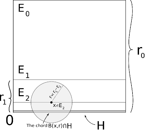
The sequence (rj)j=1N(r_{j})_{j=1}^{N} is assumed to be rapidly decreasing enough, where the rate of decay will depend on ϵ\epsilon. Some aspects of the construction are depicted in Figure 4.

Refer to caption
Figure 4. The measure μ\mu and various related objects.

We will now prove (i), namely that

∫0∞β2,μ2​(B⁡(x,r))​d​rμ⁡(B⁡(x,r))≤ϵfor all ​x∈spt⁡μ.\int_{0}^{\infty}\beta^{2}_{2,\mu}(B(x,r))\frac{dr}{\mu(B(x,r))}\leq\epsilon\quad\text{for all }x\in\operatorname{spt}\mu.

First, suppose x∈Hx\in H and r>0r>0. If r<rNr<r_{N}, we have that β2,μ2​(B⁡(x,r))=0\beta^{2}_{2,\mu}(B(x,r))=0. Another easy case is r≥r0r\geq r_{0}, and we handle it now. Then we have μ⁡(B⁡(x,r))≳1\mu(B(x,r))\gtrsim 1 and, testing with the line L=ℝ×{0}L=\mathbb{R}\times\{0\},

(4.1) β2,μ2​(B⁡(x,r))≤ϵ′​∑j=1N∫B⁡(x,r)∩Ej(rjr)2​d​ℋ1​(y)≲ϵ′​r03r2,\beta^{2}_{2,\mu}(B(x,r))\leq\epsilon^{\prime}\sum_{j=1}^{N}\int_{B(x,r)\cap E_{j}}\Big(\frac{r_{j}}{r}\Big)^{2}d\mathcal{H}^{1}(y)\lesssim\frac{\epsilon^{\prime}r_{0}^{3}}{r^{2}},

so that

∫r0∞β2,μ2​(B⁡(x,r))​d​rμ⁡(B⁡(x,r))≲ϵ′​r03​∫r0∞r−2​𝑑r=ϵ′​r02=(ϵ′)7.\int_{r_{0}}^{\infty}\beta^{2}_{2,\mu}(B(x,r))\frac{dr}{\mu(B(x,r))}\lesssim\epsilon^{\prime}r_{0}^{3}\int_{r_{0}}^{\infty}r^{-2}\,dr=\epsilon^{\prime}r_{0}^{2}=(\epsilon^{\prime})^{7}.

Let now r∈[rN,r0)r\in[r_{N},r_{0}), and specifically r∈[rj+1,rj)r\in[r_{j+1},r_{j}) for some j∈0,…,N−1j\in{0,\ldots,N-1}. We have μ⁡(B⁡(x,r))≳ϵ′​r0−1​r\mu(B(x,r))\gtrsim\epsilon^{\prime}r_{0}^{-1}r and, observing that B⁡(x,r)∩Ej=∅B(x,r)\cap E_{j}=\emptyset,

(4.2) μ(B(x,r))β2,μ2(B(x,r))≤ϵ′∑i=1N∫B⁡(x,r)∩Ei(rir)2dℋ1(y)≲ϵ′r∑i:r≥riri2≲ϵ′rrj+12,\mu(B(x,r))\beta^{2}_{2,\mu}(B(x,r))\leq\epsilon^{\prime}\sum_{i=1}^{N}\int_{B(x,r)\cap E_{i}}\Big(\frac{r_{i}}{r}\Big)^{2}d\mathcal{H}^{1}(y)\lesssim\frac{\epsilon^{\prime}}{r}\sum_{i:\,r\geq r_{i}}r_{i}^{2}\lesssim\frac{\epsilon^{\prime}}{r}r_{j+1}^{2},

so that

∫rj+1rjβ2,μ2​(B⁡(x,r))​d​rμ⁡(B⁡(x,r))≲∫rj+1rjr02(ϵ′​r)2​ϵ′r​rj+12​𝑑r≲r02ϵ′.\int_{r_{j+1}}^{r_{j}}\beta^{2}_{2,\mu}(B(x,r))\frac{dr}{\mu(B(x,r))}\lesssim\int_{r_{j+1}}^{r_{j}}\frac{r_{0}^{2}}{(\epsilon^{\prime}r)^{2}}\frac{\epsilon^{\prime}}{r}r_{j+1}^{2}\,dr\lesssim\frac{r_{0}^{2}}{\epsilon^{\prime}}.

This yields

∫rNr0β2,μ2​(B⁡(x,r))​d​rμ⁡(B⁡(x,r))≲N​r02ϵ′≲r0(ϵ′)2=ϵ′.\int_{r_{N}}^{r_{0}}\beta^{2}_{2,\mu}(B(x,r))\frac{dr}{\mu(B(x,r))}\lesssim N\frac{r_{0}^{2}}{\epsilon^{\prime}}\lesssim\frac{r_{0}}{(\epsilon^{\prime})^{2}}=\epsilon^{\prime}.

Combining the above estimates gives

∫0∞β2,μ2​(B⁡(x,r))​d​rμ⁡(B⁡(x,r))≤ϵ,x∈H,\int_{0}^{\infty}\beta^{2}_{2,\mu}(B(x,r))\frac{dr}{\mu(B(x,r))}\leq\epsilon,\qquad x\in H,

by choosing cc in ϵ′=c​ϵ\epsilon^{\prime}=c\epsilon small enough.

Let then x∈Ej0x\in E_{j_{0}}, j0=1,…,Nj_{0}=1,\ldots,N. We split

∫0∞\displaystyle\int_{0}^{\infty} β2,μ2​(B⁡(x,r))​d​rμ⁡(B⁡(x,r))\displaystyle\beta^{2}_{2,\mu}(B(x,r))\frac{dr}{\mu(B(x,r))}
=(∫0rj0−rj0+1+∫rj0−rj0+1rj0−1−rj0+∫rj0−1−rj0r0−rj0+∫r0−rj0∞)β2,μ2(B(x,r))d​rμ⁡(B⁡(x,r))\displaystyle=\Big(\int_{0}^{r_{j_{0}}-r_{j_{0}+1}}+\int_{r_{j_{0}}-r_{j_{0}+1}}^{r_{j_{0}-1}-r_{j_{0}}}+\int_{r_{j_{0}-1}-r_{j_{0}}}^{r_{0}-r_{j_{0}}}+\int_{r_{0}-r_{j_{0}}}^{\infty}\Big)\beta^{2}_{2,\mu}(B(x,r))\frac{dr}{\mu(B(x,r))}
=I+I​I+I​I​I+I​V,\displaystyle=I+II+III+IV,

and further

I​I​I=∑j=1j0−1∫rj−rj0rj−1−rj0β2,μ2​(B⁡(x,r))​d​rμ⁡(B⁡(x,r))=∑j=1j0−1I​I​Ij.III=\sum_{j=1}^{j_{0}-1}\int_{r_{j}-r_{j_{0}}}^{r_{j-1}-r_{j_{0}}}\beta^{2}_{2,\mu}(B(x,r))\frac{dr}{\mu(B(x,r))}=\sum_{j=1}^{j_{0}-1}III_{j}.

(note that I​I​I=0III=0 trivally if j0=1j_{0}=1, so we may assume that j0≥2j_{0}\geq 2 while treating I​I​IIII). If 0<r<rj0−rj0+10<r<r_{j_{0}}-r_{j_{0}+1}, then B⁡(x,r)B(x,r) intersects only one of the line segments of spt⁡μ\operatorname{spt}\mu, and β2,μ2​(B⁡(x,r))=0\beta_{2,\mu}^{2}(B(x,r))=0. Thus I=0I=0.

Another easy case is, when r≥r0−rj0r\geq r_{0}-r_{j_{0}}, which gives the same result as the case r≥r0r\geq r_{0} above, again using μ⁡(B⁡(x,r))≳1\mu(B(x,r))\gtrsim 1, testing with the line L=ℝ×{0}L=\mathbb{R}\times\{0\}, and repeating the computation from (4.1). We get I​V≲ϵ′​r02=(ϵ′)7IV\lesssim\epsilon^{\prime}r_{0}^{2}=(\epsilon^{\prime})^{7}.

The case I​III is the hardest. So we first deal with I​I​IIII by handling a fixed term I​I​IjIII_{j} for some 1≤j≤j0−11\leq j\leq j_{0}-1, in particular

(4.3) rj−rj0<r<rj−1−rj0.r_{j}-r_{j_{0}}<r<r_{j-1}-r_{j_{0}}.

We will use the following formula for the length of a chord: if S⁡(z,R2)S(z,R_{2}) is any circle of radius R2>0R_{2}>0, and JJ is a chord at distance 0<R1≤R20<R_{1}\leq R_{2} from zz, then

(4.4) ℋ1​(J)=2​R22−R12∼R2​R2−R1.\mathcal{H}^{1}(J)=2\sqrt{R_{2}^{2}-R_{1}^{2}}\sim\sqrt{R_{2}}\sqrt{R_{2}-R_{1}}.

Applying this to the chord B⁡(x,r)∩HB(x,r)\cap H of the circle S⁡(x,r)S(x,r), we obtain

μ⁡(B⁡(x,r))≥μ⁡(B⁡(x,r)∩H)=Θ⋅ℋ1​(B⁡(x,r)∩H)∼ϵ′r0​r​r−rj0∼ϵ′​rr0.\mu(B(x,r))\geq\mu(B(x,r)\cap H)=\Theta\cdot\mathcal{H}^{1}(B(x,r)\cap H)\sim\frac{\epsilon^{\prime}}{r_{0}}\sqrt{r}\sqrt{r-r_{j_{0}}}\sim\frac{\epsilon^{\prime}r}{r_{0}}.

Here the equivalence r−rj0∼rr-r_{j_{0}}\sim r follows from the left hand side of (4.3), which implies that

r−2​rj0≥rj0−1−rj0−2​rj0≥0,r-2r_{j_{0}}\geq r_{j_{0}-1}-r_{j_{0}}-2r_{j_{0}}\geq 0,

or equivalently r−rj0≥r/2r-r_{j_{0}}\geq r/2. Thus,

∫rj−rj0rj−1−rj0β2,μ2​(B⁡(x,r))​d​rμ⁡(B⁡(x,r))≲∫rj/2rj−1−rj0r02(ϵ′​r)2⋅[μ⁡(B⁡(x,r))​β2,μ2​(B⁡(x,r))]​𝑑r,\int_{r_{j}-r_{j_{0}}}^{r_{j-1}-r_{j_{0}}}\beta_{2,\mu}^{2}(B(x,r))\frac{dr}{\mu(B(x,r))}\lesssim\int_{r_{j/2}}^{r_{j-1}-r_{j_{0}}}\frac{r_{0}^{2}}{(\epsilon^{\prime}r)^{2}}\cdot[\mu(B(x,r))\beta_{2,\mu}^{2}(B(x,r))]\,dr,

and whenever 0<r<rj−1−rj00<r<r_{j-1}-r_{j_{0}}, repeating the computation from (4.2) yields

μ⁡(B⁡(x,r))​β2,μ2​(B⁡(x,r))≲ϵ′r​rj2.\mu(B(x,r))\beta^{2}_{2,\mu}(B(x,r))\lesssim\frac{\epsilon^{\prime}}{r}r_{j}^{2}.

Altogether,

I​I​Ij=∫rj−rj0rj−1−rj0β2,μ2​(B⁡(x,r))​d​rμ⁡(B⁡(x,r))≲r02ϵ′,III_{j}=\int_{r_{j}-r_{j_{0}}}^{r_{j-1}-r_{j_{0}}}\beta_{2,\mu}^{2}(B(x,r))\frac{dr}{\mu(B(x,r))}\lesssim\frac{r_{0}^{2}}{\epsilon^{\prime}},

and summing this estimate for 1≤j≤j0−11\leq j\leq j_{0}-1 gives

I​I​I=∑j=1j0−1I​I​Ij≲r0(ϵ′)2=ϵ′.III=\sum_{j=1}^{j_{0}-1}III_{j}\lesssim\frac{r_{0}}{(\epsilon^{\prime})^{2}}=\epsilon^{\prime}.

It remains to handle the case I​III, where

(4.5) rj0−rj0+1<r≤rj0−1−rj0.r_{j_{0}}-r_{j_{0}+1}<r\leq r_{j_{0}-1}-r_{j_{0}}.

We begin with the former task, so fix rr as in (4.5). Observe that

∫rj0−rj0+1rj0−rj0+1+(ϵ′)2​rj0β2,μ2​(B⁡(x,r))​d​rμ⁡(B⁡(x,r))≤∫rj0−rj0+1rj0−rj0+1+(ϵ′)2​rj01⋅d​rϵ′​r≲(ϵ′)2​rj0ϵ′​rj0=ϵ′.\int_{r_{j_{0}}-r_{j_{0}+1}}^{r_{j_{0}}-r_{j_{0}+1}+(\epsilon^{\prime})^{2}r_{j_{0}}}\beta_{2,\mu}^{2}(B(x,r))\frac{dr}{\mu(B(x,r))}\leq\int_{r_{j_{0}}-r_{j_{0}+1}}^{r_{j_{0}}-r_{j_{0}+1}+(\epsilon^{\prime})^{2}r_{j_{0}}}1\cdot\frac{dr}{\epsilon^{\prime}r}\lesssim\frac{(\epsilon^{\prime})^{2}r_{j_{0}}}{\epsilon^{\prime}r_{j_{0}}}=\epsilon^{\prime}.

It remains to handle the integration over the range

rj0−rj0+1+(ϵ′)2​rj0<r<rj0−1−rj0.r_{j_{0}}-r_{j_{0}+1}+(\epsilon^{\prime})^{2}r_{j_{0}}<r<r_{j_{0}-1}-r_{j_{0}}.

Choose rr on this interval, and note that, by requiring the decay of the sequence (ri)(r_{i}) to be so rapid that rj0+1<(ϵ′)2​rj0/2r_{j_{0}+1}<(\epsilon^{\prime})^{2}r_{j_{0}}/2, we have

(4.6) rj0+(ϵ′)2​rj02≤r<rj0−1−rj0.r_{j_{0}}+\frac{(\epsilon^{\prime})^{2}r_{j_{0}}}{2}\leq r<r_{j_{0}-1}-r_{j_{0}}.

We wish to find a lower bound for μ⁡(B⁡(x,r))\mu(B(x,r)), and this is accomplished with the aid of the chord length estimate (4.4). Namely, repeating an earlier estimate,

μ⁡(B⁡(x,r))≥μ⁡(B⁡(x,r)∩H)=Θ⋅ℋ1​(B⁡(x,r)∩H)∼ϵ′r0​r​r−rj0.\mu(B(x,r))\geq\mu(B(x,r)\cap H)=\Theta\cdot\mathcal{H}^{1}(B(x,r)\cap H)\sim\frac{\epsilon^{\prime}}{r_{0}}\sqrt{r}\sqrt{r-r_{j_{0}}}.

Note that the left hand side of (4.6) implies that

r−rj0≳(ϵ′)2​r,r-r_{j_{0}}\gtrsim(\epsilon^{\prime})^{2}r,

because this holds at r=rj0+(ϵ′)2​rj0/2r=r_{j_{0}}+(\epsilon^{\prime})^{2}r_{j_{0}}/2, the left endpoint of our interval, and the derivative of r↦r−rj0−(ϵ′)2​rr\mapsto r-r_{j_{0}}-(\epsilon^{\prime})^{2}r is positive. Hence,

μ⁡(B⁡(x,r))≳(ϵ′)2​rr0.\mu(B(x,r))\gtrsim\frac{(\epsilon^{\prime})^{2}r}{r_{0}}.

Next, we essentially repeat the computation from (4.2), recalling the upper bound r<rj0−1−rj0r<r_{j_{0}-1}-r_{j_{0}}, which means that B⁡(x,r)∩Ej0−1=∅B(x,r)\cap E_{j_{0}-1}=\emptyset:

μ⁡(B⁡(x,r))​β2,μ2​(B⁡(x,r))≤ϵ′​∑i=1N∫B⁡(x,r)∩Ei(rir)2​d​ℋ1​(y)≲ϵ′r​∑i=j0Nri2≲ϵ′r​rj02.\mu(B(x,r))\beta^{2}_{2,\mu}(B(x,r))\leq\epsilon^{\prime}\sum_{i=1}^{N}\int_{B(x,r)\cap E_{i}}\Big(\frac{r_{i}}{r}\Big)^{2}d\mathcal{H}^{1}(y)\lesssim\frac{\epsilon^{\prime}}{r}\sum_{i=j_{0}}^{N}r_{i}^{2}\lesssim\frac{\epsilon^{\prime}}{r}r_{j_{0}}^{2}.

Combining the estimates above leads to

∫rj0−rj0+1+(ϵ′)2​rj0rj0−1−rj0β2,μ2​(B⁡(x,r))​d​rμ⁡(B⁡(x,r))≲r02(ϵ′)3​∫rj0rj0−1−rj0rj02r3​𝑑r≲r02(ϵ′)3.\int_{r_{j_{0}}-r_{j_{0}+1}+(\epsilon^{\prime})^{2}r_{j_{0}}}^{r_{j_{0}-1}-r_{j_{0}}}\beta_{2,\mu}^{2}(B(x,r))\frac{dr}{\mu(B(x,r))}\lesssim\frac{r_{0}^{2}}{(\epsilon^{\prime})^{3}}\int_{r_{j_{0}}}^{r_{j_{0}-1}-r_{j_{0}}}\frac{r_{j_{0}}^{2}}{r^{3}}\,dr\lesssim\frac{r_{0}^{2}}{(\epsilon^{\prime})^{3}}.

Collecting the estimates we get

I​I≲r02(ϵ′)3+ϵ′=(ϵ′)3+ϵ′.II\lesssim\frac{r_{0}^{2}}{(\epsilon^{\prime})^{3}}+\epsilon^{\prime}=(\epsilon^{\prime})^{3}+\epsilon^{\prime}.

Combining the estimates for the terms I,…,I​VI,\ldots,IV we have

∫0∞β2,μ2(B(x,r))d​rμ⁡(B⁡(x,r))≤ϵ,x∈Ej0,j0=1,…,N,\int_{0}^{\infty}\beta^{2}_{2,\mu}(B(x,r))\frac{dr}{\mu(B(x,r))}\leq\epsilon,\qquad x\in E_{j_{0}},\,j_{0}=1,\ldots,N,

by choosing c>0c>0 small enough in ϵ′=c​ϵ\epsilon^{\prime}=c\epsilon. The proof of Theorem 1.4 is complete.

References

  • [1] Azzam, J., Tolsa, X.: Characterization of nn-rectifiability in terms of Jones’ square function: Part II. Geom. Funct. Anal. 25, 1371–1412 (2015)
  • [2] David, G., Semmes, S.: Analysis of and on uniformly rectifiable sets. In: Mathematical Surveys and Monographs 38, Amer. Math. Soc., Providence, RI (1993)
  • [3] David, G., Semmes, S.: Singular integrals and rectifiable sets in 𝐑n{\bf R}^{n}: Beyond Lipschitz graphs. Astérisque 193, 152 pp. (1991)
  • [4] Badger, M., Schul, R.: Multiscale analysis of 11-rectiable measures: necessary conditions. Math. Ann. 361, 1055-1074 (2015)
  • [5] Badger, M., Schul, R.: Two sufficient conditions for rectifable measures. Proc. Amer. Math. Soc. 144, 2445–2454 (2016)
  • [6] Badger, M., Schul, R.: Multiscale analysis of 11-rectifiable measures II: characterizations. Preprint, arXiv:1602.03823, 2016.
  • [7] Jones, P.: Rectifiable sets and the traveling salesman problem. Invent. Math. 102, 1–15 (1990)
  • [8] Lerman, G.: Quantifying curvelike structures of measures by using L2L^{2} Jones quantities. Comm. Pure Appl. Math. 56, 1294–1365 (2003)
  • [9] Tolsa, X.: Characterization of nn-rectifiability in terms of Jones’ square function: Part I. Adv. Calc. Var. 54, 3643–3665 (2015)