Tropical Igusa Invariants
Abstract
Let be a smooth geometrically connected projective curve of genus two over a complete non-archimedean field . For discretely valued , the first main theorem in [Liu93] gives a set of criteria on the Igusa invariants of the curve that determine the minimal skeleton of together with its edge lengths and vertex weights. In this paper we use the theory of Berkovich spaces to give a new proof of this theorem that works for arbitrary complete non-archimedean fields. We furthermore interpret the final result in terms of tropical moduli spaces and tropical Igusa invariants. This reformulation shows that the abstract tropicalization map factors through the tropicalization of a concrete embedding of into a weighted projective space.
1 Introduction
Let be a smooth proper curve of genus two over a complete algebraically closed non-archimedean field . An important invariant of the Berkovich analytification of is its minimal skeleton , which can be described as the set of points in that do not admit an affinoid neighborhood isomorphic to a closed disk. Alternatively, it is the dual graph of the special fiber of a stable model of together with some additional data on its edges and vertices. For curves of genus two, there are seven possible graph-theoretical types for , see Figure 1.

Our goal in this paper is to characterize the minimal skeleton in terms of the Igusa invariants of . To that end, we introduce a set of tropical Igusa invariants, which are the valuations of certain Igusa invariants. We then prove the following.
Theorem 1.1.
Suppose that the characteristic of the residue field of is not two. The tropical Igusa invariants then completely determine the minimal skeleton of a curve of genus two. The conditions that distinguish between the different reduction types are given by half-spaces.
This result is a generalization of [Liu93, Théorème 1], which proves the same result but over a complete discretely valued field. Our proof also simplifies certain aspects of the proof in [Liu93] using the framework of Berkovich spaces. For instance, we do not have to work with local affine -models, since we can use the results in [Hel21a] to deduce the skeleton from the tree of the branch locus of the hyperelliptic map . The main idea after this is as follows. For every reduction type, we write down an analytic universal family. By applying suitable Möbius transformations on the tree of the branch locus, we then find that every curve with this reduction type occurs in this family. We then compute the tropical Igusa invariants for each universal family and after some further calculations using Gröbner bases we find the statement of the theorem.
We also connect this material to the abstract theory of tropical curves of genus two found in [ACP15]. To do this, we embed the coarse moduli space into a weighted projective space using a set of Igusa invariants. The tropicalization of this embedding forms the natural target space for the tropical Igusa invariants. We then use Theorem 1.1 to define a surjective map from this tropicalization to the abstract tropicalization . The final result can be found in Corollary 2.18.
Before we start the main material of the paper, we give a short list of related papers. There is a similar result for elliptic curves using the -invariant, which says that the minimal skeleton has a cycle (of length ) if and only if . Various incarnations of this result can be found in the literature. For instance, on the tropical side this can be found in [KMM09], [BPR16] and [Hel19]. For curves of genus two, there is Liu’s paper [Liu93], which is a precursor to the current paper. Tropically, there is [CM16], which gives explicit faithful tropicalizations in some cases and a part of Theorem 1.1 (using different half-spaces).
1.1 Leitfaden
We start in Section 2.1 by recalling the concept of a skeleton of a marked curve and the action of . We then discuss the Igusa invariants, see Section 2.2. In Section 2.2.1 we tropicalize these invariants and obtain the tropical Igusa invariants. The formulas for the various reduction types and edge lengths of skeleta of curves of genus two can also be found in this section. We end Section 2.2.1 by connecting our embedded tropicalization to the abstract tropicalizations studied in [ACP15]. We then prove Theorem 1.1. This theorem is split up into two parts: 2.11 and 2.15. The first distinguishes between the various reduction types and the second gives the edge lengths for the skeleton of a given reduction type. Their proofs can be found in Sections 2.3 and 2.4 respectively.
2 The main theorem
This paper uses many concepts and results from [Hel21b] and [Hel21a] on coverings of curves; the reader is referred to those papers for more details. These papers in turn heavily rely on [ABBR15], [BPR14] and [BPR16], so we recommend reading these as well. The list below gives a short summary of the notation we use in this paper.
- •
is a complete algebraically closed non-archimedean field with valuation ring , maximal ideal and residue field .
- •
The valuation is denoted by . The absolute value associated to is , where is Euler’s number.
- •
We fix a splitting of the valuation map and write for the corresponding element of valuation , where is the value group of .
- •
We write or for a smooth irreducible proper curve over . We will also simply call this a curve. We write for its Berkovich analytification.
- •
- •
2.1 Skeleta of curves of genus two
Let be a curve over and let . We assume here that the Euler characteristic of the marked curve is negative. The marked curve then admits a unique minimal skeleton by [BPR14, Section 4.16]. By adding the genera of the type- points in , this becomes a weighted topological graph. The skeleton furthermore inherits the skeletal metric from , making it into a weighted metric graph.
Definition 2.1.
[Skeleta] The weighted metric graph associated to the marked curve is the minimal skeleton of .
We are interested in this minimal skeleton for curves of genus two with . The total genus function
| (1) |
is then equal to two. Here is the first Betti number of and is the genus of the curve associated to . This gives seven different reduction types, which can be found in Figure 1. The arrows in this figure will be discussed later.
The material in [Hel21a] characterizes the minimal skeleton of any superelliptic curve in terms of the minimal skeleton of the marked curve , where is the branch locus of the map . Here one assumes . If , then this material thus gives the minimal skeleton for curves of genus two. There are seven different tree types for which can be found in Figure 2. For each of these trees, there is a unique degree- covering ramified over its leaves (see [Hel21b]) and the covering curve has genus . The tree types in Figure 2 now match up with the corresponding reduction types given in Figure 1.

Remark 2.2.
In [RSS14], tropicalizations of various classical moduli spaces are studied. They in particular study the tropicalization of the moduli space of curves of genus two and the moduli space of projective lines with six marked points. There is a minor technical issue involving the base field however in [RSS14, Theorem 5.3]. Namely, they assume in the beginning of the paper that , which is not enough to completely remove the problem of wild ramification for the hyperelliptic covering as we can take fields of residue characteristic two, e.g., . In fact, their result becomes false in this case: the curve has tree type IV with respect to our labeling, but its reduction type is V, see [Liu93, Exemple 2]. In particular, we find that the commutative diagram given in [RSS14, Theorem 5.3.(a)] does not commute. To repair this issue, one can just assume as in this paper.
Remark 2.3.
In [CM16], curves of genus two are studied from a tropical point of view. To find the skeleton of a curve of genus two, they use the notion of a faithful tropicalization. In short, this is an embedding of into a toric variety such that its tropicalization defines an isometry of a skeleton of into the tropicalization of the toric variety. This method does not directly work for two reduction types however, see [CM16, Theorem 1.2]. They also obtain a subversion of our Theorem 1.1, determining conditions on the tropical Igusa invariants for some of the reduction types and giving formulas for the edge lengths in some cases. Our results and proofs do not encounter any of the difficulties above: we can determine the skeleton of any curve and we have a complete description of the skeleta (including the edge lengths) in terms of our tropical Igusa invariants. This method does not give a faithful embedding of the skeleton, but these can be produced abstractly using [BPR16]. Theorem 1.1 does determine the invariants (e.g. the cycle lengths) of a faithful tropicalization of however, since these only rely on the abstract minimal skeleton.
2.1.1 and trees
As before, let be a complete, algebraically closed non-archimedean field. The automorphism group of the projective line is and consequently by GAGA the automorphism group of the Berkovich analytification is also . In projective coordinates, a matrix acts by . We also refer to these as Möbius transformations. Throughout this paper, we will often use the fact that for any three distinct points in , we can find a unique such that , and . This will greatly reduce some of our computations.
Consider the hyperbolic space as in [BPR14, Section 5]. There is a natural skeletal metric on and every automorphism of acts as an isometry by the results in [BPR14, Section 2]. We now add a set of marked points to . If , then the marked curve satisfies and we thus have a unique minimal skeleton . For any automorphism , we then have . Combinatorially, we can just replace every leaf with to find .
Example 2.4.
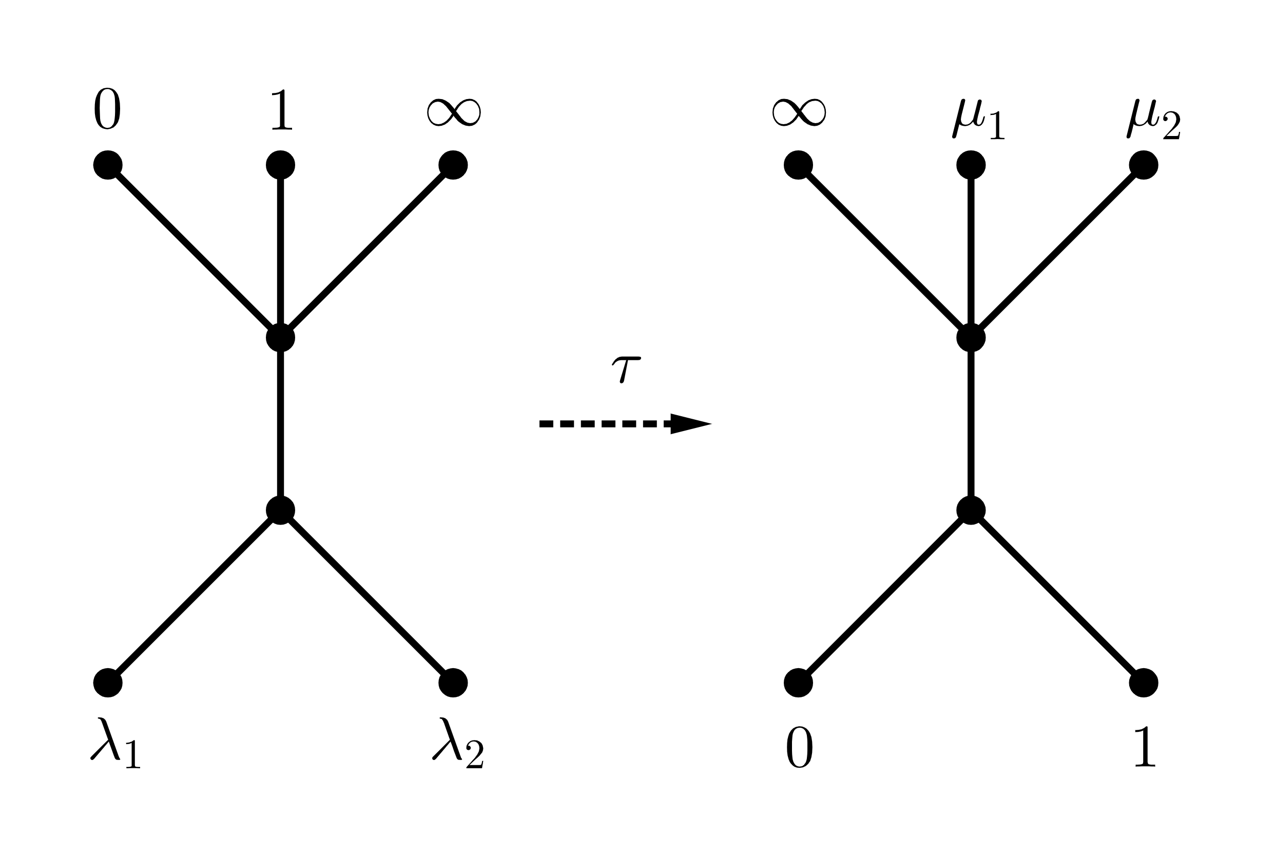
2.2 Igusa invariants
We now recall some concepts and results from [Igu60] and [Liu93] on invariants and moduli of curves of genus two. Let and write for the generic binary form of -degree over an algebraically closed field . We define a degree function on by setting . We also refer to this as the -degree. As before, any matrix in acts on through Möbius transformations. By comparing the entries of and , we then also obtain an action on . An invariant of index is a homogeneous polynomial such that for any matrix , we have . The degree of an invariant is its degree as an element of . In this paper we are interested in invariants of binary forms
of -degree . We moreover restrict ourselves to invariants of even -degree. These invariants form an algebra generated over by elements , , and of degrees , , and respectively. These are used in [Igu60] to define invariants of degree for . We refer to these polynomials as the Igusa invariants. To calculate them, we use the command in the computer algebra package MAGMA.
There is one relation between the , namely . We denote the corresponding graded algebra by 11 1 This ring is isomorphic to . and its projectivization by . We can connect these invariants to the moduli space of genus two curves as follows. Write for the functor that assigns to a scheme the set of isomorphism classes of smooth proper morphisms whose fibers are geometrically connected curves of genus two. We denote the corresponding coarse moduli space by . The Igusa invariants allow us to give this coarse moduli space explicitly: it is the open subscheme , see [Igu60, Theorem 2].
2.2.1 Tropicalizing the Igusa invariants
We now consider the algebra over a complete algebraically closed non-archimedean field . We write for the corresponding scheme. Using the grading , we can view this as a closed subscheme of the weighted projective space . Since weighted projective varieties are toric varieties, we can now define the tropicalization of with respect to this embedding, see [MS15, Chapter 6], [Gub13], [Pay09] or [Rab12]. Unfortunately, this tropicalization does not determine the abstract tropicalization of .
Example 2.5.
Let and consider the three polynomials
where , and . The valuations of the invariants are the same for and , but the lengths of the edges in the minimal skeleta of the curves and are different. The valuations of the Igusa invariants of differ from the other two by the vector . That is, they are equivalent in the corresponding tropical weighted projective space (see Definition 2.6).22 2 We can also calculate the invariants of the polynomial . The valuations of the Igusa invariants of are then the same as the valuations of the Igusa invariants of and . Note that the reduction type for and is III, but the reduction type for is VI. We thus see that the valuations of these Igusa invariants can in general detect neither the edge lengths, nor the reduction type.
To obtain the abstract tropicalization of , we extend our set of Igusa invariants as in [Liu93]. Define
If we remove the redundant factors, this gives an embedding of into . To express this tropicalization more neatly, we introduce the corresponding weighted tropical projective space.
Definition 2.6.
Let and consider the punctured tropical plane . Let be fixed. We define an action of on the punctured tropical plane by
| (2) |
The tropical weighted projective space is the set-theoretic quotient of the tropical punctured plane by this action.
Using this definition with , we arrive at our definition of the tropical Igusa invariants.
Definition 2.7.
[Tropical Igusa Invariants] The valuations of the invariants and are the tropical Igusa invariants. We view these as functions .
Remark 2.8.
If we are not interested in non-archimedean fields of residue characteristic , then we do not need to consider . The corresponding embedding of then lands in and the target space for the tropicalization becomes .
Remark 2.9.
We go back one step and review a similar construction for binary quartics and elliptic curves. As expected, this gives the tropical -invariants studied in [KMM09] and [Hel19]. For simplicity, we assume that here. The invariant ring for binary forms of -degree four admit two natural generators which are usually denoted by and . The discriminant of can then also be expressed in terms of these generators. For instance, in terms of the formulae given in [Sil09] we have . Here we view as a degenerate quartic with one zero at infinity (this is generic enough for our purposes). Consider the scheme , where , and have degrees , and respectively. We view this as a closed subscheme of the weighted projective space . The tropicalization of is and the functions , and are the tropical invariants for the quartic. The tropical -invariant is then the rational function defined on the open subscheme of .
Remark 2.10.
Returning to the Igusa invariants, we now explain where and come from. If we evaluate these invariants at the degenerate sextic , we obtain the and invariants for considered as a quartic, see the paragraph before [Liu93, Définition 1]. We will not explicitly need this fact in our proof of Theorem 1.1.
We now define the subspaces of that determine the various reduction types of genus two curves. These subspaces will be defined by homogeneous linear forms in the tropical Igusa invariants. To give linear forms that work in all residue characteristics, we first define the following:
The linear forms are now given by
Here the first subscript for all but the last three linear forms corresponds to the reduction type. Note that all these functions are tropically homogeneous, so that they give rational functions on open subsets of the tropical weighted projective space . It will follow from the proof of Theorem 2.3 that these are well defined. For instance, for curves of reduction type II, we have that is nonzero, so and we can thus evaluate the . If a given set of Igusa invariants has , then we write , so that the conditions for II in Theorem 2.11 are not satisfied.
Theorem 2.11.
[Main Theorem I] The reduction types for curves of genus two are described by the following conditions on the tropical Igusa invariants.
- I.
The reduction type is I if and only if for every .
- II.
The reduction type is II if and only if for every and .
- III.
The reduction type is III if and only if for every , , and either or .
- IV.
The reduction type is IV if and only if for every .
- V.
The reduction type is V if and only if for and .
- VI.
The reduction type is VI if and only if for , and .
- VII.
The reduction type is VII if and only if for and .
The proof of this theorem will be given in Section 2.3.
Remark 2.12.
We will only prove this when . [Liu93, Théorème 1] states that the same conditions also work for fields of residue characteristic two, but we haven’t verified this ourselves. The definition for when is an artifact of certain anomalous congruences on Igusa invariants, see part (B) of the proof of [Liu93, Théorème 1]. The reader who is not interested in these cases can just assume throughout the rest of the paper.
Remark 2.13.
The discretely valued case proven in [Liu93] can be recovered from the algebraically closed case we prove here. Indeed, if has stable reduction over , then the skeleton is stable under taking the base change to the completion of the algebraic closure.
Remark 2.14.
The tropical Igusa invariants also determine the edge lengths of the minimal skeleton of a curve of genus two. This is the content of the second part of our main theorem.
Theorem 2.15.
[Main Theorem II] The edge lengths of the minimal skeleton of a curve of genus two are given by the following.
- I.
There are no non-trivial edges.
- II.
There is one non-trivial edge of length .
- III.
Let be the lengths of the two non-trivial edges. Then
- IV.
Let be the lengths of the three non-trivial edges. Let , and . Then
- V.
There is one non-trivial edge of length
- VI.
Let be the length of the connecting edge and let the length of the cycle. Then
- VII.
Let be the length of the connecting edge and let be the lengths of the cycles. Then
The proof of this theorem will be given in Section 2.4.
Remark 2.16.
Suppose that is a curve of genus two over a discretely valued complete non-archimedean field . If has stable reduction over , then the formulas above can be used to determine the component group of the Néron model of the Jacobian of , see [Bak08]. We refer the reader to [Liu93] for explicit formulas.
We now discuss how this material connects to the abstract tropicalizations studied in [ACP15]. On the algebraic side, there is the coarse moduli space , see the beginning of Section 2.2. On the tropical side we have , which is the moduli space of tropical curves of genus two. We quickly recall its definition here, see [ACP15] for more details. Let be a weighted stable graph of genus two. We can vary the lengths of the edges in to obtain the local moduli space for tropical curves of type . We write for the closed cone corresponding to . The boundary also has a moduli space interpretation: it corresponds to reduction types obtained by contracting edges or cycles with . For every contraction , we then obtain an inclusion of closed cones . Here we also allow isomorphisms of graphs, which are in a sense degenerate contractions. The tropical moduli space for curves of genus two is then defined as the colimit over all weighted contractions. Locally this limit is quite concrete: the image of in is . Other examples of contraction morphisms for tropical curves of genus two can be found in Figure 1.
Example 2.17.
Let be the graph corresponding to reduction type IV. The corresponding open moduli space is and its image in is . Consider the sublocus of outside the diagonals, i.e., consider with , and distinct. Its image in the quotient can then be uniquely represented by triples with . These kinds of decompositions will also play a role in the proof of Theorem 1.1, see 2.4.4.
We can connect the algebraic approach to the tropical approach by introducing an abstract tropicalization map. We start with a point , which corresponds to a smooth curve of genus . The minimal skeleton of is automatically a tropical curve and the tropicalization map sends to . We now use Theorem 1.1 to relate this abstract tropicalization map to the embedded tropicalization map in 2.7. As mentioned before, the tropical Igusa invariants give us explicit coordinates on the coarse moduli space , which gives an embedding of into . We write for this embedding and for its tropicalization. Theorem 1.1 then gives a stratification of in terms of half-spaces. On the other hand, also has a natural stratification in terms of the reduction types. Our findings in Theorem 1.1 can now be summarized as follows.
Corollary 2.18.
There is a surjective map such that . This map preserves the stratifications on both sides.
Proof.
We define the map as follows. Let be a given set of tropical Igusa invariants obtained from a point in for a non-archimedean field . By Theorem 2.11, this uniquely determines a reduction type. Theorem 2.15 then gives us the edge lengths of the corresponding skeleton, which allows us to reconstruct the corresponding tropical curve. We set to be this tropical curve. This map obviously commutes with the abstract tropicalization map. For the surjectivity, we use -valued points of , where is a complete algebraically closed non-archimedean field with value group . Let be a tropical curve of genus . Using the universal families in the proof of Theorem 2.11 (see Section 2.3), we easily find a curve that tropicalizes to . The image of the corresponding point in then gives the desired set of tropical Igusa invariants. ∎
Remark 2.19.
The map not injective. For instance, the fiber over the locus of good reduction is positive dimensional: for any with , we set and find and (here we assume ).
2.3 Proof of the main theorem
We will assume throughout this section that . The main idea in the proofs of theorems 2.3 and 2.4 is as follows. As we saw earlier, there are exactly seven reduction types for curves of genus two. For every reduction type, we give a (naive) universal family, in the sense that every curve of a given reduction type is isomorphic to a member of this family. We then check the conditions in Theorem 2.11 for the members in this family to obtain the first implication. To obtain the second implication, we show that the conditions are exclusive, in the sense that the conditions for two distinct types cannot hold at the same time. Our proof for Theorem 2.15 is similar: we compare the edge lengths in the universal family to the functions in 2.15 and see that they coincide.
Remark 2.20.
Throughout our computations below, we will additionally assume for simplicity and brevity. The main difference for is that one has to use a new function that is nonzero on the universal families. More specifically, one uses instead of for the last three reduction types. This also changes the weight, so the powers for the other invariants need to be changed as well, see the equations for the half-spaces given earlier. We leave the calculation of the invariants in this case to the reader.
2.3.1 Case I: Good reduction
A curve of genus two has good reduction if and only if the phylogenetic type of the tree of the branch locus of the map is trivial, see [Hel21a, Proposition 3.13]. We now choose three points in and find a Möbius transformation such that , and , see Figure 4.

Throughout our proofs, we will use a red vertex for , a green vertex for and a blue vertex for . Our choice of now implies that the other branch points are mapped to points of valuation zero. We then similarly have and . We thus see that can be represented as
| (3) |
where the satisfy the above conditions. To put this in analytic terms, consider the scheme defined by the ring . The extra tropical conditions on the define an affinoid subdomain of and this is our naive moduli space for curves of good reduction. Using our earlier arguments we now see that every curve of good reduction arises from a type- point of . Conversely, it is not too hard to see that every type- point of this space corresponds to a curve of genus two with good reduction. We now calculate the tropical Igusa invariants for this universal family and find that (note that is just the discriminant of ). This directly shows that the inequalities in Theorem 2.11 are satisfied.
2.3.2 Case II
We choose as in Figure 5 and find a Möbius transformation such that , and .
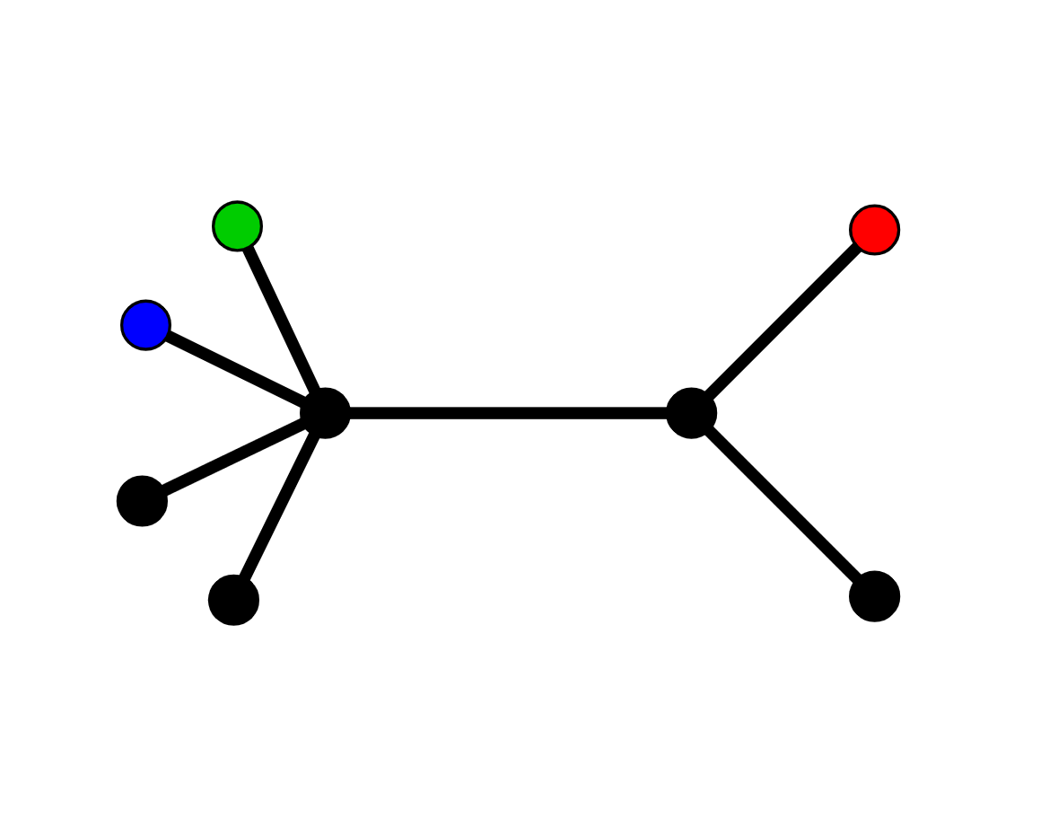
Our universal family is then given by the equation , where
| (4) |
Here we evaluate at for . The equations for the are for every , and for . We now calculate the reduction modulo of the Igusa invariant . This factorizes as
| (5) |
By the assumptions imposed on our , we find that . This directly implies that the conditions in the theorem are satisfied.
2.3.3 Case III
We choose as in Figure 6 and find a Möbius transformation such that , and .

This gives the universal family with
| (6) |
Here and are evaluated at for . We calculate the reduction of modulo and find
| (7) |
which is nonzero by our assumptions. We furthermore have
The ideal generated by and in is trivial, so these two forms cannot simultaneously be zero. This gives the conditions in the theorem.
2.3.4 Case IV
As before, we find a Möbius transformation that sends the points , and in Figure 7 to , and .

This gives the universal family with
and
We then calculate , , , , and . The reduction of modulo is , so . We furthermore find that the reductions of , and modulo are zero. This easily implies the inequalities in the theorem.
2.3.5 Case V
The universal family derived from Figure 8 is given by , where
and

We first calculate the reduction of modulo , which is . For fields with , this form would be zero, so we would have to replace it by . At any rate, we now factorize and obtain
| (8) |
We furthermore have and for and integral. We directly obtain the desired conditions from this.
2.3.6 Case VI
The universal family derived from Figure 9 is given by , where
and

The invariant is divisible by and the reduction of modulo is , which is not zero. We furthermore have and . The desired inequalities follow directly from this.
2.3.7 Case VII
The universal family derived from Figure 10 is given by , where
and

We find that , and . The reduction of modulo is , so it is always nonzero. This gives the desired inequalities.
2.3.8 Conclusion
We now combine the results of the previous sections and prove Theorem 2.11.
Proof.
The previous sections show that the indicated conditions are necessary. For the sufficiency, we show that they define exclusive conditions. We will treat most cases here and leave a few to the reader. Suppose that the conditions for I and II are both satisfied. We can assume that . We then have and consequently . This contradicts , as desired. Suppose that the conditions for I and III are both satisfied. We can assume that . The condition for implies . But then , a contradiction. This also covers the case where I and IV are both satisfied. Suppose that the conditions for II and IV are satisfied. We can suppose that , so that for . This implies by . The inequality then gives . But then either or . This contradicts , as desired. We now show that the conditions for III and IV are mutually exclusive. We suppose that . Then for . But this implies that , a contradiction.
Finally, we show that the conditions for and the conditions for the first four reduction types are mutually exclusive. We will only do this for (so ), the other cases can be checked in a similar fashion. We start with reduction type I. We can suppose again that , so that . Then must be zero, a contradiction. For reduction type II, we suppose that , so that and . But then , a contradiction. For reduction type III, we suppose that . We then have . But then , a contradiction. This also clears reduction type IV. We leave the last three remaining cases to the reader. ∎
2.4 The edge lengths
We now prove Theorem 2.15.
2.4.1 Case I
There are no non-trivial edges in this case.
2.4.2 Case II
In terms of the universal family given in 2.3.2, the edge length in the tree is given by and we have . Since the edge length is doubled, we find that the cycle has length . We moreover have , so the desired formula follows.
2.4.3 Case III
We calculate and for the universal family in 2.3.3. is divisible by and the reduction of modulo is
which is nonzero by our assumptions. The invariant is not divisible by either , but it is zero modulo . Calculating modulo monomials in the of total degree , we find that
| (9) |
We can now switch and using a projective transformation and assume that . If , then and . If , then . This gives the formulae in the theorem.
2.4.4 Case IV
The from the universal family in 2.3.4 can come in different flavors. By applying another Möbius transformation, we can however assume that . There are then four cases:
We first calculate , and . We have , and . Here the reduction of modulo is , which is always nonzero. We now calculate modulo monomials in the of total degree and find
| (10) |
We then similarly calculate modulo the monomial ideal
and find
| (11) |
Note that the monomials in are those whose "valuations" are greater than , or .
In the first of the four cases introduced above, we find that and thus . We then also find . This gives us , so we are able to express the in terms of the tropical Igusa invariants. For the second case, we find that . Using the formula for , we then also recover . In the third case we again have and one recovers from . Finally, if all the are equal, then we can find them using the formula . One now easily verifies that the formulae in the theorem hold.
2.4.5 Case V
Recall from 2.3.5 that and . This directly gives the formula in the theorem.
2.4.6 Case VI
We first calculate . We then recover from as in Section 2.3.6 and from . The formula in the theorem follows directly from this.
2.4.7 Case VII
By applying a Möbius transformation fixing , we can assume that . The reduction of modulo is , so it is nonzero. By our calculations in Section 2.3.7, we then have , so this gives the length of the connecting edge. We now calculate the reduction of modulo the ideal and obtain
| (12) |
If , then we find that and using we then also find . If , then we can use to obtain both and , as before.
References
- [ABBR15] Omid Amini, Matthew Baker, Erwan Brugallé, and Joseph Rabinoff. Lifting harmonic morphisms I: Metrized complexes and Berkovich skeleta. Springer, Research in the Mathematical Sciences, 2(1), June 2015.
- [ACP15] Dan Abramovich, Lucia Caporaso, and Sam Payne. The tropicalization of the moduli space of curves. Annales scientifiques de l’École normale supérieure, 48(4):765–809, 2015.
- [Bak08] Matthew Baker. Specialization of linear systems from curves to graphs. Algebra & Number Theory, 2(6):613–653, October 2008.
- [BPR14] Matthew Baker, Sam Payne, and Joseph Rabinoff. On the structure of nonarchimedean analytic curves. In Tropical and Non-Archimedean Geometry, volume 605, pages pp. 93–121. American Mathematical Society, 2014.
- [BPR16] Matthew Baker, Sam Payne, and Joseph Rabinoff. Nonarchimedean geometry, tropicalization, and metrics on curves. Foundation Compositio Mathematica, 3(1):63–105, jan 2016.
- [CM16] Maria Angelica Cueto and Hannah Markwig. How to repair tropicalizations of plane curves using modifications. Experimental Mathematics, 25(2):130–164, 2016.
- [Gub13] Walter Gubler. A guide to tropicalizations. In Algebraic and Combinatorial Aspects of Tropical Geometry, pages 125–189. American Mathematical Society, May 2013.
- [Hel19] Paul Alexander Helminck. Faithful tropicalizations of elliptic curves using minimal models and inflection points. Arnold Mathematical Journal, 5(4):401–434, 2019.
- [Hel21a] Paul Alexander Helminck. Invariants for trees of non-archimedean polynomials and skeleta of superelliptic curves. arXiv:2101.02918, 2021.
- [Hel21b] Paul Alexander Helminck. Skeletal filtrations of the fundamental group of a non-archimedean curve. arXiv:1808.03541, 2021.
- [Igu60] Jun-Ichi Igusa. Arithmetic variety of moduli for genus two. The Annals of Mathematics, 72(3):612, November 1960.
- [KMM09] Eric Katz, Hannah Markwig, and Thomas Markwig. The tropical j-invariant. LMS Journal of Computation and Mathematics, 12:275–294, 2009.
- [Liu93] Qing Liu. Courbes stables de genre 2 et leur schéma de modules. Mathematische Annalen, 295(2):201–222, 1993.
- [MS15] Diane Maclagan and Bernd Sturmfels. Introduction to Tropical Geometry. Graduate Studies in Mathematics. American Mathematical Society, 2015.
- [Pay09] Sam Payne. Analytification is the limit of all tropicalizations. Mathematical Research Letters, 16(3):543–556, 2009.
- [Rab12] Joseph Rabinoff. Tropical analytic geometry, Newton polygons, and tropical intersections. Advances in Mathematics, 229(6):3192–3255, 2012.
- [RSS14] Qingchun Ren, Steven V. Sam, and Bernd Sturmfels. Tropicalization of classical moduli spaces. Mathematics in Computer Science, 8(2):119–145, 2014.
- [Sil09] Joseph H. Silverman. The Arithmetic of Elliptic Curves. Springer New York, 2009.