Bin \surnameYu \urladdr \subjectprimarymsc201057R32 \subjectsecondarymsc201057M25 \arxivreferencearXiv:1604.03723 \arxivpassword
Affine Hirsch foliations on -manifolds
Abstract
This paper is devoted to discussing affine Hirsch foliations on -manifolds. First, we prove that up to isotopic leaf-conjugacy, every closed orientable -manifold admits , or affine Hirsch foliations. Furthermore, every case is possible.
Then, we analyze the -manifolds admitting two affine Hirsch foliations (abbreviated as Hirsch manifolds). On the one hand, we construct Hirsch manifolds by using exchangeable braided links (abbreviated as DEBL Hirsch manifolds); on the other hand, we show that every Hirsch manifold virtually is a DEBL Hirsch manifold.
Finally, we show that for every , there are only finitely many Hirsch manifolds with strand number . Here the strand number of a Hirsch manifold is a positive integer defined by using strand numbers of braids.
keywords
affine Hirsch foliation, classification, exchangeable braid1 Introduction
In 1975, Hirsch [Hir] constructed an analytic 2-foliation on a closed 3-manifold so that the foliation contains exactly one exceptional minimal set. Let’s briefly recall his construction here.
The foliation is constructed by starting with a solid torus and removing from the interior another solid torus which wraps around the original solid torus twice. This gives us a manifold, foliated by -punctured disks, with two transverse tori as boundary components. We then glue the exterior boundary component to the interior boundary component to obtain a foliated manifold without boundary. Hirsch chose a gluing map carefully so that the -punctured fibration structure induces a foliation and the induced foliation is analytic and contains exactly one exceptional minimal set.
There are many variations of Hirsch’s construction in the literature, for instance, Ghys [Gh], Bis-Hurder-Shive [BHS].
- •
- •
In [BHS], the authors generalize Hirsch’s construction a lot. In the -dimensional case, they generalize Hirsch’s construction by starting with a solid torus and removing from a small solid torus so that can be regarded as a tubular neighborhood of a closed twisted braid in .
Actually, it is natural to generalize these foliations to a more popular case by using braids:
- •
For every -braid whose closure is a knot, starting with a solid torus and removing from the interior a small solid torus which is a small tubular neighborhood of the closure of , we get a compact -manifold, foliated by -punctured disks, with two boundary components transverse to the -punctured disk fibration.
- •
Then we glue the exterior boundary component to the interior boundary component to obtain a foliated manifold induced by the -punctured disk fibration.
To simplify, we still call the new foliations Hirsch foliations, which are the main objects in this paper. Similarly, if the gluing map is ‘affine’ in some sense, we call the Hirsch foliation affine. More precise definitions can be found in Section 2.
There are several kinds of discussions about Hirsch foliations in the literature:
- •
Bis-Hurder-Shive [BHS] generalized Hirsch’s construction to construct analytic foliations of arbitrary codimension with exotic minimal sets.
- •
Alvarez and Lessa [AL] considered the Teichmüller space of a Hirsch foliation.
- •
Shive in his thesis [Sh] considered a conjugacy question: fixing two Hirsch foliations and , a leaf-conjugacy diffeomorphism and an integer , how to find conditions on the foliations and the map which ensure that the map is ?
In this paper, we also would like to discuss a conjugacy question. Different to what Shive did, we hope to understand the leaf-conjugacy classes of Hirsch foliations. We say two foliations and on a closed -manifold are isotopically leaf-conjugate if there exists a homeomorphism which maps every leaf of to a leaf of and is isotopic to the identity map on . We say that and are the same up to isotopic leaf-conjugacy if and are isotopically leaf-conjugate. In this paper, we will restrict ourselves to affine Hirsch foliations. The reasons why we focus on affine Hirsch foliations are the following.
- •
A Hirsch foliation always can be easily rebuilt (see Remark 4.4 ) by modifying the gluing map of an affine Hirsch foliation.
- •
Affine Hirsch foliations are natural objects in dynamical systems: the projection of the stable manifolds of a Smale solenoid attractor on the orbit space of the wandering set (by a Smale solenoid mapping on a solid torus) is an affine Hirsch foliation. A forthcoming paper [Yu] will focus on this topic.
Now we can naturally ask the following question as the main motivation for this paper.
Question 1.1.
Let be a closed -manifold, can we classify all affine Hirsch foliations up to isotopic leaf-conjugacy?
Note that Alvarez and Lessa [AL, Section 1.3] have discussed this question on the -manifolds constructed by Hirsch. As a first step to answer Question 1.1, we have:
Theorem 1.2.
Let be a closed orientable 3-manifold. Then admits , , or affine Hirsch foliations up to isotopic leaf-conjugacy.
Then one naturally would like to know:
Question 1.3.
- 1.
Which -manifolds admit a Hirsch foliation?
- 2.
Which -manifolds admit two non-isotopically leaf-conjugate affine Hirsch foliations and what are the relations between these two foliations?
Actually, to the first item of Question 1.3, on the one hand, these manifolds are very clear, i.e. everyone is precisely decided by a braid and a gluing map; on the other hand, it is not easy to describe all of these manifolds in a familiar and comfortable way. Nevertheless, we would like to give some characterizations about these -manifolds.
Proposition 1.4.
Let be a closed orientable -manifold which admits an (affine) Hirsch foliation, then:
- 1.
is a toroidal -manifold whose JSJ diagram is cyclic;
- 2.
each JSJ piece is either hyperbolic or a type Seifert manifold where and () are coprime.
We are more interested in the second item of Question 1.3. We call a -manifold a Hirsch manifold if admits two non-isotopically leaf-conjugate Hirsch foliations. Notice that the -manifold constructed by Hirsch in [Hir] actually is a Hirsch manifold. Actually, there are a lot of Hirsch manifolds, see subsection 4.2 and Proposition 4.3. The following are the reasons why we are interested in Hirsch manifolds:
- •
a Hirsch manifold has some nice symmetric structures;
- •
Hirsch manifolds and their two affine Hirsch foliations will play a central role in a class of dynamical systems: in [Yu], the author will use Hirsch manifolds and affine Hirsch foliations to discuss a kind of -stable diffeomorphisms on -manifolds whose nonwandering set is the union of a Smale solenoid attractor and a Smale solenoid repeller.
Exchangeably braided links introduced by Morton [Mor] will play a crucial role to describe Hirsch manifolds. An exchangeably braided link is a two-component link in so that each component is braided relative to the other one. More details about exchangeably braided link can be found in Section 2.
Motivated by the second item of Question 1.3, we will give two observations to describe the relationships between exchangeably braided links and Hirsch manifolds. The first observation is that for every exchangeably braided link , one can build a (unique) Hirsch manifold following a series of standard combinatorial surgeries (see Section 4). Such a Hirsch manifold is called a Hirsch manifold derived from exchangeably braided link (abbreviated as a DEBL Hirsch manifold). The second observation is that every Hirsch manifold virtually is a DEBL Hirsch manifold. More precisely,
Theorem 1.5.
Let be a Hirsch manifold. Then there exists a -covering space of , named by , so that is a Hirsch manifold derived from an exchangeably braided link (DEBL Hirsch manifold). Moreover, can be divided by where is the strand number of .
Here, the strand number of a Hirsch manifold (see Definition 4.2) is defined to be the strand number of a braid which can be used to build the Hirsch manifold .
Hirsch manifolds have the following finiteness property.
Proposition 1.6.
For every , there are only finitely many Hirsch manifolds with strand number .
In the final section (Section 5), we will build an example to show:
Proposition 1.7.
There exists a -manifold which admits a Hirsch foliation but is not a Hirsch manifold.
Proposition 1.4, Proposition 4.3, the examples in Section 4 and Proposition 1.7 imply that there exist closed oriented -manifolds , and so that,
- •
doesn’t admit any affine Hirsch foliation;
- •
admits exactly one affine Hirsch foliation;
- •
is a Hirsch manifold, i.e. admits two non-isotopically leaf-conjugate affine Hirsch foliations.
This means that every case in Theorem 1.2 can be realized (in some closed -manifold).
We can see that the results (in particular, Proposition 4.3 and Theorem 1.2) in this paper give a satisfying response to classify all Hirsch foliations. After these results, we can reduce classifying all Hirsch foliations to a classical problem in one dimensional dynamical systems: classifying degree () endomorphisms 11 1 An endomorphism on means a monotonic continuous map on on up to conjugacy. More details can be found in Remark 4.4.
2 Preliminaries
Definition 2.1.
Let be a codimension foliation on a closed oriented -manifold . is called a Hirsch foliation if there exists a torus embedded into so that,
- 1.
the path closure of , , is a compact oriented -manifold with two tori and as the boundary;
- 2.
is an -punctured disk fibration on such that each fiber is transverse to ;
- 3.
every leaf in is orientable.
By Definition 2.1, a Hirsch foliation on a closed oriented -manifold can be constructed as follows (see Figure 1 for an illustration).

- •
Choose an -braid whose closure is a knot, also can be used to represent a diffeomorphism on an -punctured disc .
- •
We denote the mapping torus of by . Notice that provides a natural -punctured disk fibration on , which provides and two -fibration structures and respectively.
- •
We suppose that is oriented. Then naturally induces an orientation on each fiber of and . We also give an orientation on which naturally induces two orientations on and respectively.
- •
Build an orientation-preserving homeomorphism which maps every fiber of to a fiber of and preserves the corresponding orientations22 2 preserves the orientations since the glued manifold should be orientable. preserves the corresponding orientations of the fibers of and since every leaf in the glued foliation should be orientable. Let . Then the -punctured disk fibration on naturally induces a Hirsch foliation on by .
There are some further comments about Hirsch foliations which are useful in the rest of the paper:
- •
also can be obtained by removing a small solid torus from a solid torus where is a small tubular neighborhood of the closure of a braid ;
- •
there is a natural quotient map where is the fiber quotient space of ;
- •
induces a map , which is called the projective holonomy map of relative to the embedded torus .
Definition 2.2.
Let be a Hirsch foliation on a closed -manifold . is called an affine Hirsch foliation if the projective holonomy map of relative to an embedded torus transverse to is topologically conjugate to the map on for some , . Here we can parameterize by .
In 1985, Morton [Mor] introduced exchangeably braided links. An exchangeably braided link is a two-component link which admits a kind of very nice symmetry: each component is braided relatively to the other one, i.e. is a closed braid in the solid torus and is a closed braid in the solid torus . Such a braid is called an exchangeable braid. Automatically, every exchangeably braided link can be regarded as the union of the closure of an exchangeable braid and an axis of the closed braid.
Morton [Mor] showed many nice properties of exchangeably braided links. For instance, he built some necessary and some sufficient conditions for exchangeability. For instance, he showed that the exchangeable braids belong to a family of braids introduced by Stallings [St].
Let’s briefly introduce Stallings’ braids and the relationships between Stallings’ braids and exchangeable braids. Certainly, the closure of an exchangeable braid is a trivial knot. But the converse is not true, i.e. if the closure of a braid is a trivial knot, is not necessarily an exchangeable braid. Actually, Stallings [St] introduced a family of braids so that for every braid in this family satisfies:
- 1.
is a trivial knot;
- 2.
there is a disk spanning which intersects the axis at exactly -points.
Morton called them Stallings braids. The set of Stallings braids is a proper subset of the union of the braids whose closure is a trivial knot. In [Mor], Morton constructed a braid 33 3 Here and below, the notations for braids are standard in braid theory (see, for instance, Birman [Bi]) which is a stalling braid but not an exchangeable braid. Therefore, the union of the exchangeable braids is a proper subset of the union of Stallings braids.
Stallings braids have a very nice characterization 44 4 A careful reader can find the characterization in the beginning of [Mor, Section ]. Under this characterization, it is easy to obtain the following finiteness property.
Proposition 2.3.
For a given , up to conjugacy, there are finitely many Stallings braids with strands number .
The following corollary is an immediate consequence of this proposition (this corollary exactly is [Mor, Corollary 1.2]).
Corollary 2.4.
- 1.
Up to conjugacy, there are finitely many exchangeable braids with strand number .
- 2.
Up to isotopy, there are finitely many exchangeably braided links with linking number .
3 Proof of Theorem 1.2
This section is devoted to proving Theorem 1.2. We will prove an equivalent form of the theorem: if a closed -manifold admits a Hirsch foliation , then up to isotopic leaf-conjugacy, admits at most two affine Hirsch foliations.

First, we give more notations and parameters (see Figure 2 as an illustration).
- •
Assume that and are the associated embedding maps, and are the corresponding induced homomorphisms.
- •
We denote the oriented simple closed curve by and denote the oriented simple closed curves by . Here, the orientations of the simple closed curves are induced by . Sometimes, we also use to represent .
- •
is chosen to be an oriented simple closed curve in which intersects at one point so that endows an orientation which is coherent to the tori of .
- •
is chosen to be the unique (up to isotopy in ) oriented simple closed curve in so that,
- 1.
intersects at one point;
- 2.
endows an orientation which is coherent to the orientation of ;
- 3.
.
- 1.
- •
If there are two oriented simple closed curves and on a torus which intersect at one point, we will use ( and are coprime) to represent an oriented simple closed curve on which wraps times around and times around .
The existence and the uniqueness of can be shown by a short computation on homology, as follows. If we choose a simple closed curve so that intersects at one point and the orientation given by is coherent to the orientation of given by , then for some . Since is nonzero in , then up to isotopy, there is a unique simple closed curve in so that . To simplify, we will use and to represent the corresponding elements in .
We collect some information about as follows, which can be obtained by Alexander duality.
Lemma 3.1.
and is generated by and . Moreover, and .
The following lemma shows that the set of all punctured disk fibrations on is quite limited.
Lemma 3.2.
Let be a -punctured disk fibration on . Assume that is a fiber of whose boundary is the union of a simple closed curve and pairwise parallel and pairwise disjoint simple closed curves in (sometimes we also use to represent ). Assume that () where and are coprime. Then there exists an orientation on which induces an orientation on and an orientation on so that , and .
Proof.
First let us prove that . If we glue a solid torus to by a gluing map so that bounds a disk in , then the glued -manifold is homeomorphic to a solid torus. On the one hand, it is obvious that . On the other hand, . Therefore, .
Secondly, we can endow an orientation which induces two orientations on and respectively so that . These orientations satisfy the requirements in the lemma and will be used in the following of the proof.
In the end, we will prove that and . Since the union of and bound a -punctured disk , . Equivalently, , then, , . We have . Recall that and are coprime, therefore, , and . ∎
Remark 3.3.
Actually, for every , there always exists an associated punctured disk fibration on . One can construct them by a standard surgery in low dimensional topology (for the surgery, see for instance, Jaco [Ja, III.14]).
From now on, , and are oriented as Lemma 3.2.
Lemma 3.4.
Let be a diffeomorphism so that and (). If is isotopic to in , then is isotopic to in and is isotopic to in .
Proof.
Lemma 3.5.
If and are two -punctured disk fibrations on with two fibers and correspondingly so that is the union of and simple closed curves which are pairwise isotopic, then is isotopic to relative to in .
Proof.
Up to isotopy, we can assume that is the union of finitely many pairwise disjoint simple closed curves . Here () is defined to be the interior of . Moreover, we assume that and is minimal up to isotopy relative to .
Firstly, we will show that every () is essential in . Otherwise, some bounds a disk in . Notice that is incompressible in , the union of and , denoted by , is a -sphere embedded in . Since is an irreducible -manifold, then bounds a -ball in . This means that we can do a surgery on in a small neighborhood of the -ball to obtain so that is isotopic to and the number of the connected components of is smaller than . This contradicts the assumption.
Then there exists a nested -punctured disk with boundary for some where is an essential simple closed curve in the interior of . Here the fact that is a nested disk means that the interior of is disjoint from . We cut along to obtain a -manifold which is homeomorphic to . Since and the fact that is a nested -punctured disk, by a simple argument on , one can obtain that also bounds a nested -punctured disk in . We define by which is an incompressible -punctured disk. Since is homeomorphic to , then is isotopic to relative to in . We can push a little into the interior of to so that the intersection number of and is strictly smaller than the intersection number of and . This contradicts the minimality. ∎
Now we deal with the trouble that maybe there are many incompressible tori in a Hirsch manifold. For this purpose, we should read more topological information about .
First, we recall some classical facts about the geometry and topology of surface bundles. Nielsen-Thurston theorem (see, for instance, Fathi-Laudenbach-Poenaru [FLP]) states that a homeomorphism on a compact surface is isotopic to one of the three types according to their dynamics: periodic, reducible and pseudo-Anosov. Thurston geometrization theorem of surface bundles (see Thurston [Th]) implies that Nielsen-Thurston theorem deeply involves the geometric structure of three dimensional manifolds as follows: the mapping torus is an irreducible -manifold, moreover,
- 1.
is hyperbolic if and only if is pseudo-Anosov;
- 2.
is Seifert-fibered if and only if is periodic;
- 3.
contains an essential torus (hence we can perform JSJ decomposition) if and only if is reducible.
In particular, in the third case, there exists a collection of essential simple closed curves in so that the suspension of these curves can be glued up by a map isotopic to to give a collection of essential tori and Klein bottles which are the collection of JSJ tori and Klein bottles. Now we formalize some facts about the geometry and topology of surface bundles as follows which will be very useful.
Lemma 3.6.
Let be a mapping torus where is a compact orientable surface and is an orientation-preserving homeomorphism on . Then,
- 1.
is an irreducible -manifold and every JSJ piece of is either hyperbolic or Seifert;
- 2.
every JSJ torus of is corresponding to an essential simple closed curve in which is periodic up to isotopy under .
Now, we come back to read some topological information about .
Lemma 3.7.
is an irreducible -manifold so that,
- 1.
every JSJ piece of is either hyperbolic or Seifert;
- 2.
the JSJ diagram of is a path;
- 3.
every Seifert piece is homeomorphic to where and () are coprime and represents the Seifert manifold whose base orbifold is a -punctured sphere with a -singularity.
Proof.
Recall that can be defined to be the mapping torus of where is an -punctured compact disk and is a homeomorphism on . Then by item of Lemma 3.6, is an irreducible -manifold so that every JSJ piece is either hyperbolic or Seifert.
By item of Lemma 3.6, every JSJ torus of is corresponding to an essential simple closed curve in which is periodic up to isotopy under . On the one side, notice that every simple closed curve in is separating, then every JSJ torus of is separating. This implies that the JSJ diagram of is a tree. On the other side, is the union of two tori, and . Combing the two sides above, one could immediately obtain that the JSJ diagram of is a path.
Let be a Seifert piece of , then is homeomorphic to a solid torus minus a small open tubular neighborhood of a closed braid . Since is Seifert, should be a periodic braid. Since every periodic homeomorphism on a disk is conjugate to a rotation (see Constantin-Kolev [CK]), up to conjugacy, should be a twisted braid. This implies that is homeomorphic to a Seifert manifold .
∎
Recall that . By Lemma 3.7, the gluing map glues the two JSJ pieces corresponding to the two ends of the JSJ diagram of (notice that the two JSJ pieces maybe are the same) and the two JSJ pieces should belong to one of the following three cases:
- 1.
both of them are hyperbolic;
- 2.
one of them is hyperbolic and the other one is Seifert;
- 3.
both of them are Seifert.
In the first two cases, it is obvious that the glued torus is a JSJ torus in . In the third case, since , one can easily check that up to isotopy, doesn’t map a regular fiber on to a regular fiber on (up to isotopy) induced by the associated Seifert pieces. Therefore, is also a JSJ torus in . Now naturally we have the following corollary.
Corollary 3.8.
Let be a closed orientable -manifold which admits a Hirsch foliation. Then every incompressible torus embedded in is a JSJ torus and the JSJ diagram of is cyclic.
Lemma 3.9.
Let be a closed -manifold which admits an affine Hirsch foliation. We have the following conclusions.
- 1.
is the union of JSJ pieces by the gluing maps and . Here the union of and is the boundary of ().
- 2.
Let be a union of the maximal pairwise disjoint, pairwise non-parallel JSJ tori of and be a Hirsch foliation on . Then, can be isotopically leaf-conjugate to so that every () is transverse to .
Proof.
Item of the lemma is a direct consequence of Corollary 3.8. We only need to prove item of the theorem.
Without loss of generality, we can suppose that () and is transverse to . Let be the union of by the gluing maps . restricted to is an -punctured disk fibration, denoted by . Since admits an -punctured disk fibration , by Corollary 3.8, every incompressible torus in the interior of is a JSJ torus. Moreover, by item of Lemma 3.6, can be isotopic to relative to so that is transverse to . Then by an easy inductive argument, in can be isotopic to relative to respectively so that every is transverse to . Equivalently, we can pertubate in relative to to which is transverse to every . Then naturally induces a foliation in so that,
- •
is isotopically leaf-conjugate to ;
- •
is transverse to every .
∎
Lemma 3.10.
Let be a closed -manifold which admits an affine Hirsch foliation . Let and be two incompressible tori in so that each of them is transverse to . We denote the path closure of by () and denote the restriction of on by which is an -punctured disk fibration on . Then .
Proof.
Without loss of generality, we can suppose that and are disjoint and non-parallel. The path closure of is the union of two compact -manifolds and . Actually, and . we denote restricted to () by which is an -punctured disk fibration on . Notice that every fiber of is the union of one fiber of and fibers of . Therefore, every fiber of is an -punctured disk. Equivalently, . Similarly, . In summary, . ∎
Definition 3.11.
Let be a closed -manifold which admits an affine Hirsch foliation and be an incompressible torus which is transverse to . We denote by the path closure of and denote restricted on by which is an -punctured disk fibration. We call the strand number of .
Remark 3.12.
The following lemma explains that “the affine property” of an affine foliation is independent of the choices of and the foliations which are isotopically leaf-conjugate to the original affine foliation.
Lemma 3.13.
Let be a closed -manifold which admits an affine Hirsch foliation . Let be a Hirsch foliation so that,
- •
is isotopically leaf-conjugate to ;
- •
is transverse to an incompressible torus in and is the path closure of .
Let be the punctured disk fibration on and be the circle fibration of restricting to . Then, the projective holonomy map of relative to an embedded torus transverse to is topologically conjugate to the map on where is the strand number of and .
Claim 3.14.
Let be a closed -manifold which admits an affine Hirsch foliation . Let and be two incompressible tori in . Let () be the path closure of , be the punctured disk fibration on and be the circle fibration of restricting to . Suppose that the projective holonomy map of relative to , , is topologically conjugate to the map on . Then, the projective holonomy map of relative to , , is also topologically conjugate to the map on .
Proof.
By Lemma 3.9, we can suppose that and are disjoint and non-parallel. Let the path closure of be the union of two compact -manifolds and such that,
- 1.
();
- 2.
is the union of and by the gluing maps and ;
- 3.
and are corresponding to and and are corresponding to .
Under these notations, and . We denote by the quotient map of the fiber quotient space of .
We can define an -covering map () as follows. For every , since can be regarded as the quotient space of the circle fibration on , we can regard as a fiber of . Also notice that is embedded into , then the fiber is in some punctured disk fiber of . Therefore, the quotient map naturally induces a map . One can easily check that is an -covering map.
We claim that which is the key observation for the proof. Now let’s check this claim. For every point (), we denote by the fiber of where stays at. Let be a point in and be a point in such that . Then one can easily show that by following the definitions of , and (). Note and . By the equalities above, we have for every .
Since is affine, we can endow a suitable metric on such that and for some (). Since is an -covering map, we also can endow a metric on such that and for every . Moreover, by the fact that , we have . ∎
Proposition 3.15.
Let be an incompressible torus on a closed -manifold . We denote by the path closure of , so that is the union of and . Then up to isotopic leaf-conjugacy, there exists at most one affine Hirsch foliation so that is transverse to and is a punctured disk fibration so that each fiber of intersects at one connected component.
Proof.
We assume that and are two affine Hirsch foliations on which satisfy the conditions in the proposition. Let and be the punctured disk fibrations induced by and on respectively. Suppose is the gluing map so that .
() is a -fibration on . Similarly, is a -fibration on . We denote a fiber of (resp. , , ) by (resp. , , ). Then, up to isotopy, and . By Lemma 3.4, is isotopic to in and is isotopic to in . Then, we can suppose that , denoted by . Here is a circle fibration on .
Since each of and is an affine Hirsch foliation, by Lemma 3.13, the projective holonomy maps of and of relative to are conjugated by an orientation preserving homeomorphism , i.e. .
Recall that is a natural quotient map where is the fiber quotient space of . One can lift to a homeomorphism so that,
- •
is isotopic to the identity map on ;
- •
.
Since is isotopic to the identity map on , we can extend to a homeomorphism which is isotopic to the identity map on . Assume that is also an affine Hirsch foliation on . Let be the punctured disk fibrations induced by on . By and , one can quickly check that the boundaries of and are coherent, i.e. for every fiber , there exists a fiber so that . Then by Lemma 3.5, one can build a homeomorphism so that,
- •
is isotopic to the identity map on relative to ;
- •
.
can automatically induce a homeomorphism on so that,
- •
for every in the interior of ;
- •
is isotopic to the identity map on ;
- •
.
In summary, is a homeomorphism on so that,
- •
is isotopic to the identity map on ;
- •
.
∎
Now we can finish the proof of Theorem 1.2, i.e. up to isotopic leaf-conjugacy, a closed orientable -manifold admits at most two affine Hirsch foliations.
Proof of Theorem 1.2.
Let be an affine Hirsch foliation and be an incompressible torus in . By Lemma 3.9, we can suppose that is transverse to . We denote the path closure of by and the boundary of by the union of and . Then, is a punctured disk fibration on . has the following two possibilities:
- 1.
each leaf of intersects to at one connected component;
- 2.
each leaf of intersects to at one connected component.
In every case, by Proposition 3.15, up to isotopic leaf-conjugacy, there exists at most one affine Hirsch foliation. The conclusion of the theorem follows. ∎
4 Hirsch manifolds and exchangeably braided links
In this section, we will focus on the study of Hirsch manifolds, i.e. the closed -manifolds which admit two non-isotopically leaf-conjugate affine Hirsch foliations. First, we will introduce or recall some notations (see Figure 3 as an illustration55 5 In the case of the figure, . To avoid misunderstanding, we should point it out that generally, we can think but may not be isotopic to .) which are useful below:
- •
: an affine Hirsch foliation transverse to in ;
- •
: , and is the gluing homeomorphism;
- •
: induces oriented simple closed curves in and in which are defined at the beginning of Section 3.
- •
: (), an oriented simple closed curve in ;
- •
: , an oriented simple closed curve in ;
- •
: pairwise disjoint oriented simple closed curves which are parallel to in ;
- •
: an oriented punctured disk in so that is the union of and ;
- •
: an oriented punctured disk fibration on with a fiber ;
- •
: and .
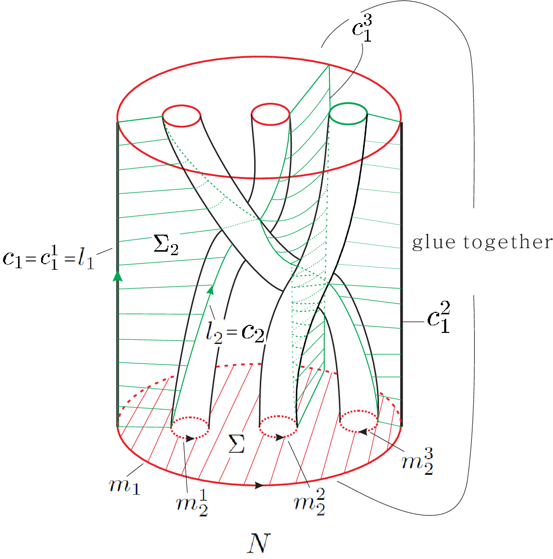
4.1 Homology and Hirsch manifolds
In this subsection, for every two nonzero integers and , we will use to represent their greatest positive common divisor.
Lemma 4.1.
Suppose also induces an affine Hirsch foliation on under . Then, , , , and .
Proof.
Since , in . Equivalently, . Recall that and , then, . Recall that . Then,
| (1) |
By filling a solid torus to along , we obtain a new compact -manifold so that bounds a disk in , then is homeomorphic to a solid torus. Following the gluing surgery, we have
Then we have,
| (2) |
Denote to be the homomorphism induced by . Notice that also induces an affine Hirsch foliation on . Then, on the one hand,
on the other hand,
Therefore,
| (3) |
∎
We can use the strand number of a braid which build a (affine) Hirsch foliation on to be an invariant of . The strand number of is well defined. Let us explain a little bit more. Maybe there are two braids to build the same Hirsch manifold , by Lemma 3.10, Definition 3.11 and Lemma 4.1, the strand numbers of the braids are the same.
Definition 4.2.
Let be a Hirsch manifold. The strand number of a braid which builds a (affine) Hirsch foliation on is called the strand number of .
Proposition 4.3.
Let and be two affine Hirsch foliations defined as above on a Hirsch manifold . Then and are not isotopically leaf-conjugate.
Proof.
Otherwise, we assume that there exists a homeomorphism which maps every leaf of to a leaf of and is isotopic to the identity map on . One can check that every leaf on is homeomorphic to either a sphere minus a Cantor set or a torus minus a Cantor set. We choose a leaf on which is homeomorphic to a sphere minus a Cantor set. We denote by which is a leaf on .
Let be the natural quotient map. By the construction of , without loss of generality, we can assume that is an oriented simple closed curve on . is homotopically nontrivial in because of the compressibility of in . Since is isotopic to the identity map on , is also homotopically nontrivial in . By the construction of , is homotopic to in for some nonzero integer . Here is the simple closed curve on . We choose an oriented closed curve in which is homotopic to in . Then and are homotopic in . This means that there exists an immersion map and an orientation on so that,
- •
and where and are oriented which are coherent to the orientation of ;
- •
is transverse to where is the interior of .
Moreover, under some pertubation of close to if it is necessary, we can assume that there exists a neighborhood of , denoted by , satisfies that . Then, is the union of finitely many, pairwise disjoint oriented simple closed curves where and . Here the orientation of () is coherent to the orientation of in . We can assume that is minimal in the following sense: let be an immersion which satisfies the conditions above, then contains at least connected components. If some is inessential in , then bounds a disk in . This means that is homotopically trivial in . Since and is incompressible in , is homotopically trivial in . Then by some standard surgery, one can build another which satisfies the conditions above and whose intersection circle number is less than . It contradicts the assumption for . Therefore, from now on, we can suppose that each is essential in . Since is an annulus, are pairwise parallel in .
Without loss of generality, we can assume that the union of cuts to open annuli so that,
- •
();
- •
.
Therefore, and are homotopic in for every . We choose a very small tubular neighborhood of in . Then belongs to one of the two sides of in . The two cases for the position of and the relations above induce two kinds of “homotopy chain relation”. We denote by where and . In both cases, we can assume that there exist oriented closed curves in and in so that:
- •
and ();
- •
and are homotopic in ().
In one case, and ; in the other case, and .
We will get contradictions in both cases by using homology theory. For every oriented closed curve in , we will use to represent the corresponding homological element in . Recall that which is generated by and (Lemma 3.1). Moreover, and . These facts will be used several times in the following.
In the first case, on the one hand, since and are homotopic in , in ; on the other hand, since is an oriented closed curve in , then for two integers and . These two sides imply that in . Notice that , then the equality is impossible. Therefore, we obtain a contradiction.
Now we discuss the second case. Since and are homotopic in (), . In particular, . Since is an oriented closed curve in , then for two integers and . We have . Therefore, and . This implies that and are homotopic in . Notice that and , then and are homotopic in . By some similar arguments, we have that and are homotopic in for every . Also notice that , and are pairwise homotopic, then and are homotopic in . This implies that . By Lemma 4.1, . Since is nonzero, then . We obtain a contradiction.
Then, the proposition is followed.
∎
Remark 4.4.
By Definition 2.1 and Definition 2.2, we can see that for a given -manifold ,
- •
on the one hand, every Hirsch foliation can be obtained from a unique affine Hirsch foliation by replacing the projective holonomy map on by another degree endomorphism on ;
- •
on the other hand, for every affine Hirsch foliation and every degree endomorphism on , one can build a Hirsch foliation with the projective holonomy map .
Moreover, by Proposition 4.3 and Theorem 1.2, one can classify all of the affine Hirsch foliations on a given -manifold .
Therefore, our results conclude the question classifying all Hirsch foliations to a classical field on one dimensional dynamical system: classifying degree () endomorphisms on up to conjugacy.
4.2 DEBL Hirsch manifolds
To be more convenient to understand the materials in this subsection, we suggest the reader to look at Figure 4.

Let be an exchangeably braided link in . We choose two disjoint small open tubular neighborhoods and of and respectively. is defined to be . so that and . The linking number of and is defined to be . is a closed -braid relative to and is a closed -braid relative to .
Up to isotopy, there is a unique way to choose a simple closed curve in and simple closed curves in so that,
- •
() bounds a disk in and is isotopic to in ;
- •
and bound an -punctured disk in .
Similarly, up to isotopy, there is a unique way to choose a simple closed curve in and simple closed curves in so that,
- •
() bounds a disk in and is isotopic to in ;
- •
and bound an -punctured disk in .
Moreover, up to isotopy, we can extend () to an -punctured disk fibration on so that,
- •
and which are two -fibrations on and ;
- •
and transversely intersects every where on ;
- •
and transversely intersects every where on .
We can suppose that the intersection number of and is and the intersection number of and (for every ) is . Similar to the beginning of Section 2 and Section 3, we would like to provide some orientations on these objects:
- •
give an orientation;
- •
and are oriented by the orientation of ;
- •
give the leaves of and some orientations continuously so that:
- 1.
every fiber of and () is oriented which is induced by the orientation of and ;
- 2.
the orientation of is coherent to and the orientation of is coherent to .
- 1.
Then, one can build an orientation preserving homeomorphism so that,
- •
and ;
- •
maps every fiber of to a fiber of ;
- •
maps every fiber of to a fiber of ;
- •
and induce two affine Hirsch foliations and on under where .
Notice that to ensure the glued manifold can admit two Hirsch foliations induced by and , up to isotopy, we can suppose that and . This implies that under this restriction, the glued manifold is unique up to homeomorphism. Therefore, we can say that an exchangeably braided link decide a unique Hirsch manifold. Every Hirsch manifold built in this way is called a Hirsch manifold derived from an exchangeably braided link (abbreviated as a DEBL Hirsch manifold).
By the second item of Corollary 2.4, we have the following consequence.
Corollary 4.5.
For every , there are only finitely many DEBL Hirsch manifolds with strand number .
4.3 A virtual property of Hirsch manifolds
Let be a Hirsch manifold. By the definition of Hirsch manifold and Lemma 3.9, there exist two affine Hirsch foliations and on and a JSJ torus in which satisfy the propositions in Lemma 3.9. Let be the path closure of , then
- •
admits two -punctured disk fibrations and and we can parameterize some subsets of as Section 2;
- •
the two Hirsch foliations and can be induced by and and a gluing map respectively.
which is generated by and . We denote the abelization homomorphism from to by and denote the quotient homomorphism from to so that and by . The kernel of , , is a normal subgroup of . Here, the definitions and properties of , () and can be found in the beginning of Section 4 and Lemma 4.1.
As a subgroup of , induces an -covering space of by a covering map . We collect some useful properties as the following. One can prove the proposition by some routine checks. We omit the details here.
Proposition 4.6.
()
- 1.
is an -punctured disk fibration on ;
- 2.
Let be a connected component of , then is a homeomorphism so that ;
- 3.
is a -covering map;
- 4.
Let be a connected component of , then is a homeomorphism so that ;
- 5.
intersects at one point.
Lemma 4.7.
There is a homeomorphism so that,
- 1.
;
- 2.
and ;
Proof.
By Proposition 4.6, () is one point, which can be defined by . We denote by , then .
Then by the classical homotopy lifting theorem, we can build a unique map so that,
- 1.
, ;
- 2.
.
Now one can automatically check that is a homeomorphism. ∎
We denote () by . and are defined to be the corresponding quotient maps.
Lemma 4.8.
There is a unique map so that for every . Furthermore, is a -covering map.
Proof.
For every , can be defined as follows. Since is surjective, there exists so that . Define . The first item of Lemma 4.7 ensures that is well defined. The uniqueness of is because of the fact that has no freedom in where .
Finally, since is a -covering map, is also a -covering map. ∎
Lemma 4.9.
is a Hirsch manifold which admits two affine Hirsch foliations and so that () is induced by under , i.e. maps each leaf of to a leaf of .
Proof.
Assume that and which are two -fibrations on and respectively. Since induces on under the gluing homeomorphism , maps every fiber of to a fiber of .
Suppose and are the lifted fibrations of and on and under the covering map respectively. is the lifted map of , i.e. . Therefore, maps every every fiber of to a fiber of . Then, induces a Hirsch foliation on .
To finish the proof, now we only need to check that is an affine Hirsch foliation. This actually is a consequence of the following facts:
- •
is the lifted map of ;
- •
is an affine Hirsch foliation;
- •
every expanding map on is topologically conjugate to an affine map on with the same degree.
∎
Lemma 4.10.
is a DEBL Hirsch manifold.
Proof.
We glue two solid tori and to along its boundary respectively by the gluing maps and so that, bounds a disk in and bounds a disk in . Then, the glued manifold is homeomorphic to .
Let () be a simple closed curve in so that is a tubular neighborhood of .
Since is a punctured disk fibration structure on and bounds a disk in , the union of and , named by , is also homeomorphic to a solid torus. Obviously, is a closed braid in . Since , automatically, is a closed braid relative to , i.e. is a closed braid in .
Similarly, one can show that is a closed braid relative to . Therefore, is an exchangeably braided link. Now one can automatically build the Hirsch manifold derived from and check that the Hirsch manifold is homeomorphic to . ∎
4.4 Finiteness of Hirsch manifolds with stand number
We will use the following theorem of Wang [Wang].
Theorem 4.11.
Let be a closed irreducible -manifold which is nonorientable or Seifert fibered or has a nontrivial torus decomposition (i.e. there is a JSJ torus). Then covers infinitely many nonhomeomorphic 3-manifolds if and only if M is an orientable Seifert fiber space with nonzero Euler number.
proof of Proposition 1.6.
On the one hand, By Proposition 1.4, an -strand Hirsch manifold is an irreducible orientable closed -manifold with some JSJ tori. By Theorem 4.11, for an given DEBL Hirsch manifold , there are only finitely many Hirsch manifolds with as a finite covering space.
On the other hand, Corollary 2.4 says that for a positive integer , up to isotopy, there are only finitely many exchangeably braided links with strands number . Recall that an exchangeably braided link decide a DEBL Hirsch manifold. Therefore, there are only finitely many DEBL Hirsch manifolds with strand number .
Let be a Hirsch manifold with strand number . Then by Theorem 1.5, a finite covering space of , , is a DEBL Hirsch manifold with strand number . Combing the two sides above, up to homeomorphism, there are only finitely many Hirsch manifolds with strand number . ∎
5 Proof of Proposition 1.7
In this section, we will construct an example to prove Proposition 1.7, i.e. there exists a -manifold which admits an affine Hirsch foliation but is not a Hirsch manifold. We will use the following inequality by Bennequin [Be]:
Lemma 5.1 (Bennequin inequality).
Let be a non-separating link of components, presented by a closed braid with strands and () positive (negative) crossings. Then , the genus of , is bounded as follows:
Proof of Proposition 1.7.
Let be a -strand braid. Now we can follow the beginning of Section 2 to build an affine Hirsch foliation on a closed -manifold . We briefly recall the construction here.
- •
also can be used to represent a diffeomorphism on a -punctured disc and we denote the mapping torus of by .
- •
provides a -punctured disk fibration on , which provides and two -fibration structures and respectively.
- •
After carefully choosing orientations to the objects above, we can build an orientation-preserving homeomorphism which maps every fiber of to a fiber of and preserves the corresponding orientations.
- •
Let . Then naturally induces a Hirsch foliation on by . If we choose suitably, is an affine Hirsch foliation.
Now we assume that is a Hirsch manifold. Following the arguments in subsection 4.3, there exists some integer so that the braid is an exchangeable braid where is a -strand full twist braid. This means that the knot , the closed braid of , is a trivial knot. In the following, we will show that the genus of , , is nonzero. Then isn’t a trivial knot. We obtain a contradiction. Then isn’t a Hirsch manifold.
Acknowledgments
The author would like are grateful to Sébastien Alvarez for useful discussions. The author is supported by the National Natural Science Foundation of China (grant no. 11471248).
References
- [AL] S. Alvarez, P. Lessa, The Teichmüller space of the Hirsch foliation. arXiv:1507.01531v1.
- [Be] D. Bennequin, Entrelacements et èquations de Pfaff. Third Schnepfenried geometry conference, Vol. 1 (Schnepfenried, 1982), 87-161, Astérisque, 107-108, Soc. Math. France, Paris, 1983.
- [BHS] A. Biś, S. Hurder, J. Shive, Hirsch foliations in codimension greater than one. Foliations 2005, 71-108, World Sci. Publ., Hackensack, NJ, 2006.
- [Bi] J. Birman, Braids, links, and mapping class groups. Annals of Mathematics Studies, No. 82. Princeton University Press, Princeton, N.J.; University of Tokyo Press, Tokyo, 1974.
- [CK] A. Constantin, B. Kolev, The theorem of Kerékjártó on periodic homeomorphisms of the disc and the sphere, Enseign. Math. (2) 40 (1994) 193-204.
- [FLP] A. Fathi, F. Laudenbach, V. Poenaru, editors, Travaux de Thurston sur les surfaces. (French) [The works of Thurston on surfaces], Séminaire Orsay. With an English summary. Astérisque, 66-67. Société Mathématique de France, Paris, 1979.
- [Gh] E. Ghys, Topologie des feuilles génériques. (French) [Topology of generic leaves] Ann. of Math. (2) 141 (1995), no. 2, 387-422.
- [Hir] M. Hirsch, A stable analytic foliation with only exceptional minimal sets. in Dynamical Systems, Warwick, 1974, Lect. Notes in Math., 468, Springer-Verlag, 1975, 9¨C10.
- [Ja] W. Jaco, Lectures on three-manifold topology. CBMS Regional Conference Series in Mathematics, 43. American Mathematical Society, Providence, R.I., 1980.
- [Mor] H. R. Morton Exchangeable braids. Low-dimensional topology (Chelwood Gate, 1982), 86-105, London Math. Soc. Lecture Note Ser., 95, Cambridge Univ. Press, Cambridge, 1985.
- [Ro] D. Rolfsen, Knots and Links. Corrected reprint of the 1976 original. Mathematics Lecture Series, 7. Publish or Perish, Inc., Houston, TX, 1990.
- [Sh] J. H. Shive, Conjugation problems for Hirsch foliations. Ph.D thesis, University of Illinois at Chicago, 2005.
- [St] J. H. Stallings, Constructions of fibred knots and links. Algebraic and geometric topology (Proc. Sympos. Pure Math., Stanford Univ., Stanford, Calif., 1976), Part 2, pp. 55-60, Proc. Sympos. Pure Math., XXXII, Amer. Math. Soc., Providence, R.I., 1978.
- [Th] W. P. Thurston, Hyperbolic structures on -manifolds, : Surface groups and -manifolds which fiber over circle. arxiv:math.GT/9801045.
- [Wang] S. Wang, -manifolds which cover only finitely many 3 -manifolds. Quart. J. Math. Oxford Ser. (2) 42 (1991), no. 165, 113-124.
- [Yu] B. Yu, Smale solenoid attractors and affine Hirsch foliations. In preparation.