Robust regression for optimal individualized treatment rules
Abstract: Because different patients may response quite differently to the same drug or treatment, there is increasing interest in discovering individualized treatment rule. In particular, people are eager to find the optimal individualized treatment rules, which if followed by the whole patient population would lead to the “best” outcome. In this paper, we propose new estimators based on robust regression with general loss functions to estimate the optimal individualized treatment rules. The new estimators possess the following nice properties: first, they are robust against skewed, heterogeneous, heavy-tailed errors or outliers; second, they are robust against misspecification of the baseline function; third, under certain situations, the new estimator coupled with pinball loss approximately maximizes the outcome’s conditional quantile instead of conditional mean, which leads to a different optimal individualized treatment rule comparing with traditional Q- and A-learning. Consistency and asymptotic normality of the proposed estimators are established. Their empirical performance is demonstrated via extensive simulation studies and an analysis of an AIDS data.
Key words and phrases: Optimal individualized treatment rules; Personalized medicine; Quantile regression; Robust regression.
1 Introduction
Given the same drug or treatment, different patients may respond quite differently. Factors causing individual variability in drug response are multi-fold and complex. This has raised increasing interests of individualized medicine, where customized medicine or treatment is recommended to each individual according to his/her characteristics, including genetic, physiological, demographic, environmental, and other clinical information. The rule that applied in personalized medicine to match each patient with a target treatment is called individualized treatment rule (ITR), and our goal is to find the “optimal” one, which if followed by the whole patient population would lead to the “best” outcome. For many complex diseases such as cancer and AIDS, the optimal individualized treatment rule or regime is a dynamical treatment process, involving a sequence of treatment decisions made at different time points throughout the disease evolving course.
Q-learning (Watkins and Dayan,, 1992; Murphy,, 2005) and A-learning (Murphy,, 2003; Robins,, 2004) are two main approaches for finding optimal dynamic individualized treatment rules based on clinical trials or observational data. Q-learning is based on posing a regression model to estimate the conditional expectation of the outcome at each time point, and then applying a backward recursive procedure to fit the model. A-learning, on the other hand, only requires modeling the contrast function of the treatments at each time point, is therefore more flexible and robust to a model misspecification. See Schulte et al., (2014) for a complete review and comparison of these two methods under various scenarios, in terms of the parameter estimation accuracy and the estimation of expected outcomes. Q- and A-learning have good performance when model is correctly specified but are sensitive to model misspecification. To overcome this shortcoming, several “direct” methods have been proposed, which maximize value functions directly instead of modeling the conditional mean. See Zhao et al., (2012); Zhang et al., (2013) for example.
All existing methods for optimal individualized treatment rule estimation, including Q-learning and A-learning, belong to mean regression as they estimate the optimal estimator by maximizing expected outcomes. In the case of single decision point, Q-learning is equivalent to the least-squares regression. Least-squares estimates are optimal if the errors are i.i.d. normal random variables. However, skewed, heavy-tailed, heteroscedastic errors or outliers of the response are frequently encountered. In such situations, the efficiency of the least square estimates is impaired. One extreme example is that when the response takes i.i.d. Cauchy errors, neither Q-learning nor A-learning can consistently estimate the optimal ITR. For example, in AIDS Clinical Trials Group Protocol 175 (ACTG175) data (Hammer et al.,, 1996), HIV-infected subjects were randomized to four regimes with equal probabilities, and our objective is to find the optimal ITR for each patient based on their age, weight, race, gender and some other baseline measurements. The response CD4 count of the data follows a skewed, heteroscedastic errors, which weakens the efficiency of classical Q- and A-learning. A method to estimate optimal ITR which is robust against skewed, heavy-tailed, heteroscedastic errors or outliers is highly valuable. One possible solution is to construct the optimal decision rule based on the conditional median or quantiles of response given covariates than based on average effects.
In the following, we present a simple example where a quantile-based decision rule is more preferable than a mean-based decision rules. We use higher value of response to indicate more favorable outcomes. Figure 1 plots the conditional density of under two treatments, and , given a binary covariate which takes the value of male and female. Under the comparison based on conditional means, and are exactly equivalent. However, conditional quantiles provide us more insight. For the male group, the conditional distribution of response given treatment is a log-normal and skewed to the right. Therefore, treatment is less favorable when either 50% or 25% conditional quantile are considered. For the female group, the conditional distribution of response given treatment is a standard normal while a Cauchy distribution given treatment . Therefore, if we make a comparison based on conditional quantile, treatment is more favorable.
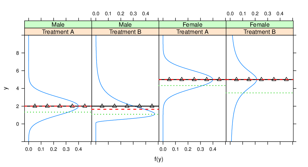
In this paper, we propose a general framework for optimal individualized treatment rule estimation based on robust regression, including quantile regression and the regression based on Huber’s loss and -insensitive loss. The proposed methodology has the following desired features. First, the new decision rule obtained by maximizing the conditional quantile, which is suitable for skewed, heavy-tailed errors or outliers. Second, the proposed estimator requires only modeling the contrast function between two treatments, and is therefore robust against misspecification of the baseline function. This property is shared by A-learning. Third, empirical results from our comprehensive numerical study suggest favorable performance of the new robust regression estimator.
The rest of the paper is organized as follows. In Section 2, we first review the classical Q- and A- learning methods. Then we propose the new procedure and method and discuss its connection with existing methods. In Section 3, we study and prove the asymptotic properties of the proposed method, including consistency and asymptotic normality. In Section 4, a comprehensive numerical study is conducted to assess finite sample performance of the new procedure. In Section 5, we apply the method to ACTG175 data. Concluding remarks are given in Section 6. Throughout the paper, we use upper case letters to denote random variables and lower case letters to denote their values.
2 New Optimal Treatment Estimation Framework: Robust Regression
2.1 Basic Notations and Assumptions
For simplicity, we consider a single stage randomized clinical trial with two treatments. For each patient, the observed data is , where denotes the baseline covariates, denotes the treatment assigned to the patient, and is the real-valued response, which is coded so that higher values indicate more favorable clinical outcomes. An ITR is a function mapping from to .
We first review the potential outcome framework (Neyman,, 1923; Rubin,, 1974; Rubin,, 1986). The potential outcome is the outcome for an arbitrary individual has s/he received treatment . In actuality, at most one of the potential outcomes can be observed for any individual. The optimal ITR under mean regression, which maximizes the expected outcome, is . Define the propensity score . Following Rubin, (1974) and Rubin, (1986), we can compute the expectation of the potential outcome under the following two key assumptions.
- (C1)
Stable Unit Treatment Value Assumption (SUTVA): a patient’s observed outcome is the same as the potential outcome for the treatment that s/he actually received. Based on Rubin, (1986), the SUTVA assumption implies that the value of the potential outcome for a subject does not depend on what treatments other subject receive. Specifically, we can write the SUTVA assumption as
(1) This is also referred as consistency assumption.
- (C2)
Strong Ignorability Assumption: the treatment assignment for an individual is independent of the potential outcomes conditional on the covariates , i.e., . For a randomized clinical trial, this assumption is satisfied automatically. For an observational study, as clinicians make decisions based only on all past available information, this assumption essentially assumes no unmeasured confounders.
For consistent estimation of the optimal treatment rule, we also need to assume
- (C3)
Positivity Assumption: , .
2.2 Existing Learning Methods: Q-learning and A-learning
Define the Q-function . Under assumptions (C1)-(C2), one can show that . This suggests that, in order to find , we only need to estimate the conditional expectation of given . This result serves as the foundation of Q- and A-learning framework. We further define the value function which is simply the marginal mean outcome under the ITR , and .
Define the -th conditional quantile of given as . Then we define the value function based on the -th conditional quantile as , which is an analog to the definition of . The optimal ITR which maximizes the -th conditional quantile is then defined as
| (2) |
and .
Consider the general model , where represents the baseline effect, and denotes the contrast effect as
Therefore, }. In Q-learning, a parametric model is often employed as a working model,
| (3) |
where and are posited parametric models for and respectively. Commonly a linear model is assumed for simplicity and interpretability, i.e., and , where . Given the observation , the Q-learning procedure estimates the parameters by minimizing the squared error loss
| (4) |
Denote the optimized point as . The estimated optimal ITR based on Q-learning is then , which is a consistent estimator of if both and are correctly specified.
A-learning is a semiparametric improvement of Q-learning by modeling only the contrast function rather than the full Q-function. This is reasonable based on the observation that the optimal ITR only depends on . By positing for the contrast function, in A-learning, one can estimate coefficients by solving the following estimating equation
| (5) |
where and are arbitrary functions, and has the same dimension as . Denote the solution to (5) by . If is constant and is correctly specified, the optimal choices of and are and (Robins,, 2004). In practice, one may pose models, say and for and respectively, and take . Under randomized designs, the propensity score is known. Otherwise, a logistic model can be proposed. Under the assumption that is correctly specified, the double robustness property of A-learning states that as long as one of and is correctly specified, is consistent estimator of .
Recently, Lu et al., 2011 (2011) propose a variant of A-learning by a loss-based learning framework. Rewrite
where . Based on the expression above, Lu et al., (2011) propose to estimate by minimizing the following loss function
| (6) |
where , are proposed models for and respectively. Denote the minimizer of (6) as . Lu et al., (2011) show that is a consistent estimator of when the propensity score is known or can be consistently estimated from the data, and is correctly specified. We refer to this method as least square A-learning (lsA-learning).
One main advantage of the lsA-learning, compared to the classical A-learning, is its square loss, making the procedure easy to be coupled with penalized regression to achieve variable selection in high dimensional data. Specifically, Lu et al., (2011) propose to identify important nonzero coefficients in by applying an adaptive LASSO penalty to (6). Under some regularity conditions, both the selection consistency and asymptotic normality of the estimator are established in Lu et al., (2011). The downside of lsA-learning is that one direction of the double robustness property of the classical A-learning is lost, i.e., when is correctly specified, may still not be consistent if the propensity score is not consistently estimated. Finally, it can be shown that lsA-learning and Q-learning are equivalent when is constant and both and take the linear form (with the space of included in the space of ). Similar properties hold for A-learning and Q-learning (Schulte et al.,, 2014).
2.3 New Proposal: Robust Regression
Skewed, heavy-tailed, heteroscedastic errors or outliers of the response are frequently encountered in clinical trials. It is well known that ordinary least square estimation fails to produce a reliable estimator in such situations. The immediate consequence is the efficiency loss in the estimators produced by Q-, A-, and lsA-learning. This motivates us to adopt robust regression techniques in optimal treatment regime estimation.
We consider the following additive model,
| (7) |
where is the baseline function, is the contrast function, is the propensity score, and is the error term which satisfies the conditional independence assumption . We point out that the error term defined in (7) can be very general. For example, we could take for any that allows the error distribution to change with , used to model heterogeneous errors, where are arbitrary positive functions and for all . Throughout the paper, we assume are i.i.d random samples of the population.
We propose to estimate by minimizing
| (8) |
where , and is a convex function with minimum achieved at 0. Denote the minimizer of (17) as , and the estimated ITR is then . In the following, we refer the robust regression with loss function as RR(M)-learning. In this article, we consider the following three types of loss functions, i.e., the pinball loss
| (9) |
where , the Huber loss
| (10) |
for some , and the -insensitive loss
| (11) |
for some . The pinball loss are frequently applied for quantile regression (Koenker,, 2005), and the Huber losses and the -insensitive are robust against heavy tailed errors or outliers. A dramatic difference of pinball loss, Huber loss and -insensitive loss, compared with the square loss, is that they penalize large deviances linearly instead of quadratically. This property makes them more robust when dealing with responses with non-normal type of errors.
3 Asymptotic Properties
3.1 Consistency of Robust Regression: Pinball Loss
Under the conditional independence assumption , we have
where and denote the mean and the -th quantile of conditional on respectively. Therefore, in this situation, we have . In other words, the underlying ITR which maximize the population mean and -th quantile are equivalent. For a good ITR , it is reasonable to require to be a consistent estimator of . This consistency result is first shown for the robust regression with pinball loss, which is given in Theorem 1. We allocate all the proofs into the Appendix A.
Theorem 1.
Remarks:
- 1.
Theorem 1 doesn’t assume the finiteness of . Therefore it can be applied to the cases when follows a Cauchy distribution.
- 2.
After fitting the model, the Assumption (A2), , can be verified by applying conditional independence test with and given , where is the estimated residual and . See Lawrance, (1976); Su and White, (2007); Song, (2009); Huang, (2010); Zhang et al., 2012b () for more discussion of conditional independence hypothesis tests. In particular, we demonstrate the usefulness of the test by applying the Kernel-based conditional independence test (KCI-test, Zhang et al., 2012b ()) in Section 5. KCI-test doesn’t assume functional forms among variables and thus suits our need.
When the conditional independence assumption () does not hold, may no longer be a consistent estimator of . This is intuitively reasonable as contains extra information with respect to . In fact, a general result which can be derived in this case is that, minimizes a weighed mean-square error loss function with specification error (Angrist et al., 2006, 2006; Lee, 2013, 2013).
Instead of assuming response takes an additive error term as in (7), we assume the conditional quantile function , where we redundantly represent the baseline function and contrast function as and respectively. Notice that we use instead of to emphasize that the true may vary with respect to . The proposed model is with correctly specified. Define
| (12) |
where is any fixed point in . Define the QR specification error as . Define the quantile-specific residual as with conditional density function . Then we have the following approximation theorem. The proof of the theorem follows Theorem 1 of Angrist et al., (2006), and is omitted for brevity.
Theorem 2.
Suppose that (i) the conditional density exists a.s.; (ii) and are finite; (iii) uniquely solves (12). Then
| (13) |
where
| (14) |
Remarks:
- 1.
Theorem 2 shows that is a weighted least square approximation to . In other word, is close to . So even though it is not true that holds exactly, the difference between them is small in general . This coupled with the fact that (proved in Theorem 4), leads to the conclusion that approximately ITR maximizes the -th conditional quantile. This observation is justified numerically in Section 4.2.
- 2.
When there exists such that , then we have .
3.2 Consistency of Robust Regression: Other Losses
3.3 Asymptotic Normality: Pinball Loss
Without loss of generality, in this section we assume both the and take the linear form: and , where . Denote and . Denote , , and . Under the following regularity conditions, which is the same as the assumptions assumed in Angrist et al., (2006) and Lee, (2013), we have the asymptotic normality of , which is given in Theorem 4.
- (B1)
are i.i.d random variables;
- (B2)
the conditional density exists, and is bounded and uniformly continuous in y, uniformly in over the support of ;
- (B3)
is positive definite for all , where is uniquely defined in (12);
- (B4)
for some .
Theorem 4.
If regularity conditions (B1)-(B4) are hold, we have
- 1.
(Uniform Consistency) ;
- 2.
(Asymptotic Normality) converge in distribution to a zero mean Gaussian process with covariance function defined as
(15)
The proof is given in Angrist et al., (2006), and the asymptotic covariance matrix of can be estimated by either a bootstrap procedure (Hahn,, 1997) or a nonparametric kernel method (Angrist et al.,, 2006). We adopt the parametric bootstrap approach to estimate the asymptotic covariance matrix in Section 5. Under model (7) the result of Theorem 4 can be further simplified, which is given in Theorem 5.
Theorem 5.
Under the condition of Theorem 4, if further we assume , and , then
- 1.
;
- 2.
, where
Furthermore, we have .
Comparing the asymptotic normality of with yields interesting insights. Assuming that and , the asymptotic normality property of can then be established, which is summarized in Theorem 6. Its proof has been omitted, and readers are referred to Lu et al., (2011).
Theorem 6.
Remarks:
- 1.
When the family of functions cannot well approximate the unknown baseline function , the term in the asymptotic variance of may explode, which makes less efficient than .
- 2.
When , , and , the asymptotic variance of is , which is strictly larger than (the asymptotic variance of ).
4 Numerical Results: Simulation Studies
To demonstrate finite sample performance of the proposed robust regression methods for optimal treatment rule estimation, we conduct two simulation studies: the errors independent with treatments, and the errors interactive with treatments, respectively.
4.1 Simulation Study I: error terms independent with treatment
We consider the following two models with p=3,
- •
Model I:
where are multivariate normal with mean 0, variance 1, and , and .
- •
Model II:
where , and , and are the same as Model I.
We take linear forms for both the baseline and the contrast functions, where and . We assume the propensity scores are known, and we study both the constant case and the non-constant case . In addition, We consider two different functions, i.e., the homogeneous case with , and the heterogenous case with . The simulation results under constant and non-constant propensity scores are similar. Thus, for brevity, we only report the constant case and allocate the result of non-constant case to the Appendix B. The results of Model I and II with constant propensity score are given in Table 1 and 2 respectively.
| Homogeneous Error | ||||||||||
|---|---|---|---|---|---|---|---|---|---|---|
| Normal | Log-Normal | Cauchy | ||||||||
| n | method | mse | PCD | mse | PCD | mse | PCD | |||
| 100 | LS | 1.32 (0.040) | 80.7 | 1.06 | 2.36 (0.081) | 75.7 | 1.57 | 58.4 | 3.75 | |
| P(0.5) | 1.44 (0.042) | 80.1 | 1.13 | 1.73 (0.051) | 78.0 | 1.31 | 2.69 (0.077) | 75.2 | 1.63 | |
| P(0.25) | 1.90 (0.057) | 78.3 | 1.34 | 1.63 (0.051) | 79.0 | 1.29 | 5.29 (0.168) | 70.4 | 2.25 | |
| Huber | 1.15 (0.034) | 81.9 | 0.93 | 1.45 (0.044) | 79.9 | 1.13 | 2.61 (0.072) | 74.9 | 1.66 | |
| 200 | LS | 0.68 (0.021) | 85.6 | 0.59 | 1.10 (0.033) | 82.0 | 0.91 | 58.7 | 3.70 | |
| P(0.5) | 0.73 (0.021) | 85.3 | 0.62 | 0.78 (0.021) | 84.1 | 0.70 | 1.23 (0.037) | 81.3 | 0.99 | |
| P(0.25) | 0.92 (0.028) | 84.0 | 0.75 | 0.70 (0.023) | 86.0 | 0.59 | 2.48 (0.079) | 75.7 | 1.64 | |
| Huber | 0.58 (0.017) | 86.8 | 0.50 | 0.66 (0.018) | 85.5 | 0.58 | 1.24 (0.035) | 80.8 | 1.03 | |
| 400 | LS | 0.33 (0.009) | 90.3 | 0.26 | 0.56 (0.016) | 87.1 | 0.46 | 59.2 | 3.61 | |
| P(0.5) | 0.35 (0.010) | 90.0 | 0.29 | 0.37 (0.010) | 89.0 | 0.34 | 0.56 (0.016) | 87.1 | 0.48 | |
| P(0.25) | 0.43 (0.013) | 89.1 | 0.34 | 0.33 (0.010) | 90.7 | 0.25 | 1.16 (0.037) | 82.9 | 0.86 | |
| Huber | 0.28 (0.008) | 91.1 | 0.22 | 0.31 (0.009) | 90.2 | 0.27 | 0.58 (0.017) | 86.7 | 0.49 | |
| 800 | LS | 0.17 (0.005) | 93.2 | 0.13 | 0.26 (0.008) | 90.9 | 0.23 | 59.4 | 3.59 | |
| P(0.5) | 0.17 (0.005) | 93.1 | 0.13 | 0.19 (0.005) | 92.1 | 0.17 | 0.29 (0.009) | 90.7 | 0.24 | |
| P(0.25) | 0.22 (0.007) | 92.4 | 0.16 | 0.18 (0.006) | 93.6 | 0.12 | 0.59 (0.019) | 87.3 | 0.48 | |
| Huber | 0.14 (0.004) | 93.8 | 0.11 | 0.16 (0.005) | 93.1 | 0.14 | 0.29 (0.008) | 90.5 | 0.25 | |
| Heterogenous Error | ||||||||||
| Normal | Log-Normal | Cauchy | ||||||||
| n | method | mse | PCD | mse | PCD | mse | PCD | |||
| 100 | LS | 3.24 (0.110) | 74.7 | 1.70 | 8.98 (0.561) | 68.6 | 2.44 | 56.2 | 4.05 | |
| P(0.5) | 1.70 (0.060) | 80.5 | 1.08 | 1.80 (0.064) | 80.1 | 1.08 | 3.45 (0.124) | 75.1 | 1.69 | |
| P(0.25) | 2.50 (0.085) | 77.4 | 1.42 | 2.51 (0.079) | 76.8 | 1.46 | 9.13 (0.341) | 67.2 | 2.66 | |
| Huber | 1.70 (0.057) | 80.4 | 1.10 | 1.87 (0.063) | 79.2 | 1.16 | 4.27 (0.155) | 72.8 | 1.93 | |
| 200 | LS | 1.54 (0.050) | 80.6 | 1.06 | 4.71 (0.244) | 73.4 | 1.85 | 55.2 | 4.17 | |
| P(0.5) | 0.78 (0.028) | 86.7 | 0.53 | 0.90 (0.032) | 85.3 | 0.63 | 1.49 (0.052) | 81.9 | 0.95 | |
| P(0.25) | 1.16 (0.039) | 83.5 | 0.81 | 1.23 (0.039) | 82.0 | 0.91 | 3.95 (0.150) | 73.2 | 1.90 | |
| Huber | 0.77 (0.025) | 86.4 | 0.55 | 0.94 (0.032) | 84.5 | 0.69 | 1.94 (0.071) | 79.3 | 1.19 | |
| 400 | LS | 0.80 (0.026) | 86.0 | 0.58 | 2.69 (0.136) | 77.8 | 1.34 | 54.7 | 4.26 | |
| P(0.5) | 0.39 (0.013) | 90.5 | 0.27 | 0.44 (0.017) | 89.6 | 0.32 | 0.71 (0.024) | 86.9 | 0.50 | |
| P(0.25) | 0.56 (0.019) | 88.8 | 0.37 | 0.66 (0.020) | 86.9 | 0.50 | 1.70 (0.055) | 79.6 | 1.17 | |
| Huber | 0.38 (0.012) | 90.4 | 0.27 | 0.48 (0.017) | 88.8 | 0.36 | 0.91 (0.029) | 84.9 | 0.65 | |
| 800 | LS | 0.41 (0.013) | 89.9 | 0.29 | 1.35 (0.150) | 83.1 | 0.82 | 56.5 | 4.00 | |
| P(0.5) | 0.18 (0.006) | 93.6 | 0.12 | 0.20 (0.007) | 92.6 | 0.16 | 0.36 (0.013) | 91.0 | 0.25 | |
| P(0.25) | 0.28 (0.009) | 92.2 | 0.18 | 0.31 (0.010) | 90.8 | 0.24 | 0.89 (0.031) | 85.8 | 0.60 | |
| Huber | 0.19 (0.006) | 93.3 | 0.13 | 0.22 (0.007) | 92.1 | 0.18 | 0.47 (0.017) | 89.2 | 0.34 | |
| Homogeneous Error | ||||||||||
|---|---|---|---|---|---|---|---|---|---|---|
| Normal | Log-Normal | Cauchy | ||||||||
| n | method | mse | PCD | mse | PCD | mse | PCD | |||
| 100 | LS | 0.24 (0.006) | 91.1 | 0.21 | 1.23 (0.061) | 82.4 | 0.87 | 58.6 | 3.73 | |
| P(0.5) | 0.36 (0.010) | 89.0 | 0.32 | 0.39 (0.012) | 88.8 | 0.34 | 0.80 (0.024) | 84.2 | 0.69 | |
| P(0.25) | 0.45 (0.012) | 87.8 | 0.40 | 0.13 (0.004) | 93.4 | 0.12 | 2.37 (0.083) | 76.0 | 1.49 | |
| Huber | 0.25 (0.007) | 90.8 | 0.22 | 0.31 (0.010) | 90.3 | 0.26 | 0.99 (0.029) | 82.4 | 0.84 | |
| 200 | LS | 0.11 (0.003) | 93.7 | 0.10 | 0.52 (0.018) | 87.3 | 0.45 | 58.7 | 3.69 | |
| P(0.5) | 0.17 (0.005) | 92.4 | 0.16 | 0.17 (0.005) | 92.4 | 0.15 | 0.32 (0.009) | 89.5 | 0.30 | |
| P(0.25) | 0.20 (0.005) | 91.8 | 0.18 | 0.06 (0.002) | 95.6 | 0.05 | 1.03 (0.033) | 82.1 | 0.88 | |
| Huber | 0.12 (0.003) | 93.6 | 0.11 | 0.13 (0.003) | 93.5 | 0.12 | 0.43 (0.013) | 87.9 | 0.40 | |
| 400 | LS | 0.05 (0.001) | 95.7 | 0.05 | 0.26 (0.008) | 90.7 | 0.23 | 59.4 | 3.60 | |
| P(0.5) | 0.09 (0.002) | 94.5 | 0.08 | 0.09 (0.002) | 94.5 | 0.08 | 0.15 (0.004) | 92.8 | 0.14 | |
| P(0.25) | 0.10 (0.002) | 94.2 | 0.09 | 0.03 (0.001) | 96.9 | 0.02 | 0.44 (0.012) | 87.9 | 0.39 | |
| Huber | 0.06 (0.001) | 95.5 | 0.05 | 0.06 (0.002) | 95.4 | 0.06 | 0.21 (0.006) | 91.6 | 0.19 | |
| 800 | LS | 0.03 (0.001) | 96.9 | 0.03 | 0.13 (0.004) | 93.5 | 0.11 | 59.4 | 3.58 | |
| P(0.5) | 0.04 (0.001) | 96.1 | 0.04 | 0.04 (0.001) | 96.2 | 0.04 | 0.07 (0.002) | 95.1 | 0.06 | |
| P(0.25) | 0.05 (0.001) | 95.8 | 0.05 | 0.01 (0.000) | 97.9 | 0.01 | 0.20 (0.005) | 91.5 | 0.19 | |
| Huber | 0.03 (0.001) | 96.8 | 0.03 | 0.03 (0.001) | 96.8 | 0.03 | 0.10 (0.002) | 94.2 | 0.09 | |
| Heterogenous Error | ||||||||||
| Normal | Log-Normal | Cauchy | ||||||||
| n | method | mse | PCD | mse | PCD | mse | PCD | |||
| 100 | LS | 1.97 (0.072) | 79.8 | 1.13 | 7.75 (0.514) | 70.4 | 2.22 | 56.4 | 4.02 | |
| P(0.5) | 0.84 (0.029) | 86.1 | 0.55 | 1.21 (0.045) | 84.3 | 0.74 | 1.82 (0.071) | 80.5 | 1.07 | |
| P(0.25) | 1.37 (0.049) | 82.1 | 0.90 | 1.56 (0.051) | 80.5 | 1.04 | 6.20 (0.261) | 69.8 | 2.25 | |
| Huber | 0.84 (0.031) | 85.9 | 0.57 | 1.33 (0.046) | 82.8 | 0.85 | 2.69 (0.106) | 77.0 | 1.42 | |
| 200 | LS | 0.99 (0.035) | 84.7 | 0.66 | 4.16 (0.237) | 75.2 | 1.62 | 55.1 | 4.19 | |
| P(0.5) | 0.41 (0.014) | 90.2 | 0.28 | 0.58 (0.024) | 89.4 | 0.37 | 0.79 (0.030) | 86.7 | 0.52 | |
| P(0.25) | 0.64 (0.021) | 87.4 | 0.45 | 0.74 (0.024) | 86.1 | 0.54 | 2.48 (0.096) | 76.9 | 1.40 | |
| Huber | 0.39 (0.013) | 90.3 | 0.27 | 0.69 (0.027) | 87.7 | 0.45 | 1.17 (0.044) | 83.4 | 0.78 | |
| 400 | LS | 0.51 (0.018) | 89.0 | 0.35 | 2.48 (0.133) | 79.3 | 1.20 | 54.7 | 4.25 | |
| P(0.5) | 0.20 (0.007) | 93.2 | 0.14 | 0.29 (0.011) | 92.6 | 0.17 | 0.32 (0.011) | 91.2 | 0.22 | |
| P(0.25) | 0.30 (0.009) | 91.3 | 0.22 | 0.39 (0.012) | 89.9 | 0.28 | 0.99 (0.030) | 83.0 | 0.78 | |
| Huber | 0.20 (0.007) | 93.2 | 0.14 | 0.34 (0.012) | 91.4 | 0.22 | 0.53 (0.016) | 88.4 | 0.37 | |
| 800 | LS | 0.25 (0.008) | 92.2 | 0.17 | 1.25 (0.159) | 84.2 | 0.73 | 56.4 | 4.00 | |
| P(0.5) | 0.10 (0.004) | 95.3 | 0.07 | 0.14 (0.006) | 94.7 | 0.09 | 0.16 (0.006) | 93.9 | 0.11 | |
| P(0.25) | 0.14 (0.005) | 94.0 | 0.10 | 0.18 (0.006) | 92.9 | 0.14 | 0.49 (0.015) | 88.0 | 0.39 | |
| Huber | 0.09 (0.004) | 95.3 | 0.06 | 0.17 (0.006) | 93.9 | 0.11 | 0.26 (0.009) | 91.8 | 0.19 | |
Comparison is made among four methods. They are: lsA-learning, robust regression with (RR()), robust regression with (RR()), and robust regression with Huber loss (RR(H)). The error terms are taken as standard i.i.d. normal, log-normal or Cauchy distribution, and independent with both and . It is easy to check that the conditional independence assumption is satisfied, and . We consider four different sample sizes 100, 200, 400 and 800. To evaluate the performance of each method, we compare three groups of criteria: (1) the mean squared error (mse), which measures the distance between estimated parameters and the true parameter ; (2) the percentage of making correct decisions (PCD), which are calculated based on a validation set with 10000 observations. Specifically, we take the formula with ; (3) the differences of and between the optimal ITR and the estimated ITR, where and , . and (defined in Section 2.1) are estimated from the validation set as well, and they evaluate the overall performance of an ITR , where the former one focuses on the response’s mean and the latter one focuses on the response’s conditional -th quantile. Under our setting, when they both exists. Thus, only is reported. For each scenario, we take 1000 replications. All numbers in the tables are based on the sample average of all replications. We further report the standard errors of mse to evaluate the variability of the corresponding statistics.
When the propensity score is constant, lsA-learning is equivalent to both Q- and A-learning under our setting. If we compare the performance of the methods under homogeneous and heterogeneous errors, the first thing we find is that lsA-learning works much worse under the heterogeneous errors, while all other methods are generally less affected by the heterogeneity of the errors. When the baseline function is misspecified as in Model I, under the homogeneous normal errors, RR(H) works slightly better than lsA-learning, while works the worst. However, the difference in general is small. For the homogeneous log-normal errors, again RR(H) works the best, while and have similar performance, and lsA-learning works the worst. Under the homogeneous Cauchy errors, works the best and RR(H) has a close performance. The lsA-learning is no longer consistent, and its mse explodes. The actual numbers are too large and thus leave as blank in Table 1 and 2. Furthermore, with the Cauchy errors, the PCD of lsA-learning are less than 60% under all scenarios, while other methods’ PCD can be as high as 90%. When baseline function is correctly specified as in Model II, under homogeneous normal errors, lsA-learning performs the best. However, in this case RR(H) also has a very close performance, and thus makes no difference from a practical point of view to choose between these two methods. The results of Model II under other cases draw similar conclusion as Model I. To sum up, the overall conclusion is that, under the conditional independence assumption, the proposed robust regression method RR(M) is more efficient than Q-, A- and lsA-learning in the circumstances when observations have skewed, heterogeneous or heavy-tailed errors. On the other hand, when the error terms indeed follows i.i.d. normal distribution, the loss of efficiency of RR(M) is not significant. This is especially true when Huber loss is applied.
4.2 Simulation Study II: error terms interactive with treatment
We consider the following model with p=2,
where , , , and are i.i.d. Uniform[-1,1].
Similar as Section 4.1, we take linear forms for both the baseline and the contrast functions, where , and . , 10 or 15. The error terms follows i.i.d. N(0,1) or Gamma(1,1)-1 distribution. The propensity scores are known, and we consider both the constant case and the non-constant case . We report only the result of the constant case (Table 3), and allocate the non-constant case to Appendix B.
| Least Square | Pinball(0.5) | Pinball(0.25) | Huber | |||||||||||
|---|---|---|---|---|---|---|---|---|---|---|---|---|---|---|
| Error | n | |||||||||||||
| Normal | 5 | 100 | 0.16 | 0.16 | 0.31 | 0.16 | 0.16 | 0.27 | 0.25 | 0.25 | 0.17 | 0.14 | 0.14 | 0.26 |
| 200 | 0.09 | 0.09 | 0.24 | 0.10 | 0.10 | 0.19 | 0.18 | 0.18 | 0.09 | 0.08 | 0.08 | 0.19 | ||
| 400 | 0.05 | 0.05 | 0.18 | 0.07 | 0.07 | 0.12 | 0.15 | 0.15 | 0.05 | 0.05 | 0.05 | 0.13 | ||
| 800 | 0.02 | 0.02 | 0.14 | 0.05 | 0.05 | 0.09 | 0.14 | 0.14 | 0.04 | 0.03 | 0.03 | 0.09 | ||
| 10 | 100 | 0.28 | 0.28 | 0.92 | 0.22 | 0.22 | 0.81 | 0.39 | 0.39 | 0.40 | 0.21 | 0.21 | 0.82 | |
| 200 | 0.19 | 0.19 | 0.85 | 0.15 | 0.15 | 0.71 | 0.33 | 0.33 | 0.28 | 0.13 | 0.13 | 0.72 | ||
| 400 | 0.12 | 0.12 | 0.79 | 0.10 | 0.10 | 0.60 | 0.30 | 0.30 | 0.23 | 0.09 | 0.09 | 0.63 | ||
| 800 | 0.06 | 0.06 | 0.73 | 0.07 | 0.07 | 0.50 | 0.27 | 0.27 | 0.22 | 0.06 | 0.06 | 0.54 | ||
| 15 | 100 | 0.35 | 0.35 | 1.55 | 0.25 | 0.25 | 1.40 | 0.47 | 0.47 | 0.62 | 0.26 | 0.26 | 1.43 | |
| 200 | 0.27 | 0.27 | 1.48 | 0.18 | 0.18 | 1.31 | 0.45 | 0.45 | 0.45 | 0.18 | 0.18 | 1.34 | ||
| 400 | 0.19 | 0.19 | 1.47 | 0.13 | 0.13 | 1.17 | 0.44 | 0.44 | 0.37 | 0.12 | 0.12 | 1.23 | ||
| 800 | 0.12 | 0.12 | 1.39 | 0.09 | 0.09 | 1.03 | 0.41 | 0.41 | 0.35 | 0.08 | 0.08 | 1.07 | ||
| Gamma | 5 | 100 | 0.15 | 0.18 | 0.31 | 0.15 | 0.11 | 0.16 | 0.22 | 0.12 | 0.09 | 0.12 | 0.09 | 0.15 |
| 200 | 0.09 | 0.12 | 0.26 | 0.10 | 0.06 | 0.10 | 0.18 | 0.08 | 0.05 | 0.08 | 0.05 | 0.09 | ||
| 400 | 0.05 | 0.07 | 0.21 | 0.08 | 0.03 | 0.07 | 0.16 | 0.06 | 0.04 | 0.06 | 0.02 | 0.07 | ||
| 800 | 0.02 | 0.04 | 0.17 | 0.07 | 0.03 | 0.06 | 0.15 | 0.06 | 0.03 | 0.05 | 0.02 | 0.07 | ||
| 10 | 100 | 0.26 | 0.33 | 0.90 | 0.22 | 0.16 | 0.54 | 0.39 | 0.13 | 0.27 | 0.22 | 0.14 | 0.50 | |
| 200 | 0.19 | 0.29 | 0.88 | 0.17 | 0.08 | 0.44 | 0.37 | 0.10 | 0.22 | 0.17 | 0.07 | 0.41 | ||
| 400 | 0.12 | 0.24 | 0.87 | 0.13 | 0.04 | 0.39 | 0.35 | 0.08 | 0.19 | 0.14 | 0.03 | 0.36 | ||
| 800 | 0.06 | 0.17 | 0.78 | 0.12 | 0.03 | 0.37 | 0.33 | 0.07 | 0.19 | 0.13 | 0.02 | 0.35 | ||
| 15 | 100 | 0.36 | 0.57 | 1.52 | 0.30 | 0.31 | 0.98 | 0.53 | 0.19 | 0.40 | 0.32 | 0.28 | 0.89 | |
| 200 | 0.28 | 0.53 | 1.51 | 0.22 | 0.19 | 0.81 | 0.55 | 0.16 | 0.29 | 0.24 | 0.16 | 0.71 | ||
| 400 | 0.19 | 0.47 | 1.50 | 0.17 | 0.13 | 0.73 | 0.57 | 0.15 | 0.26 | 0.21 | 0.11 | 0.63 | ||
| 800 | 0.11 | 0.43 | 1.50 | 0.15 | 0.11 | 0.71 | 0.58 | 0.15 | 0.24 | 0.18 | 0.09 | 0.62 | ||
We compare the performance of four methods: lsA-learning, robust regression with (), robust regression with () and robust regression with Huber loss (). We consider four different sample sizes 100, 200, 400 and 800. For each scenario, we again simulate 1000 replications. When error terms are interactive with treatment, the true associated with and are different. Specifically, under our model, for , for and for . Thus, the two criteria, mse and PCD used in simulation study I, are no longer meaningful. So we evaluate the performance of methods in this simulation study based on value differences , and .
Based on Theorem 6, we can prove that is consistent which converges to as sample size goes to infinity. This is shown in Table 3 such that the column for the lsA-learning method converges to 0 as sample size increases. We also know under Normal error terms, . Thus, the column for the lsA-learning method also converges to 0. However, all other columns in Table 3 converge to a positive constant instead of 0 as sample size goes to infinity.
Another observation we discover from Table 3 is and perform similarly. One additional observation we have is even though lsA-learning outperform all other methods in when sample size is large. It may be worse than and when sample size is small. This is due to the fact that lsA-learning is inefficient under the heteroscedastic or skewed errors. The last observation we have is overall lsA-learning, and perform best at the columns , and accordingly. The reason is given in the Remark under Theorem 14, which shows that in general approximates the unknown optimal ITR even when the conditional independence assumption does not hold.
5 Application to AIDS study
We illustrate the proposed robust regression method to data from AIDS Clinical Trials Group Protocol 175 (ACTG175), which has been previously studied by various authors (Leon et al., 2003, 2003; Tsiatis et al., 2008, 2008; Zhang et al., 2008, 2008; Lu et al., 2011, 2011). In the study, 2139 HIV-infected subjects were randomized to four different treatment groups in equal proportions, and the treatment groups are zidovudine (ZDV) monotherapy, ZDV + didanosine (ddI), ZDV + zalcitabine, and ddI monotherapy. Following Lu et al., (2011), we choose CD4 count at weeks post-baseline as the primary continuous outcome , and include five continuous covariates and seven binary covariates as our covariates. They are: 1. age (years), 2. weight (kg), 3. karnof=Karnofsky score (scale of 0-100), 4. cd40=CD4 count at baseline, 5. cd80=CD8 count at baseline, 6. hemophilia=hemophilia (0=no, 1=yes), 7. homosexuality=homosexual activity (0=no, 1=yes), 8. drugs=history of intravenous drug use (0=no, 1=yes), 9. race (0=white, 1=non-white), 10. gender (0=female, 1=male), 11. str2= antiretroviral history (0=naive, 1=experienced), and 12. sympton=symptomatic status (0=asymptomatic, 1=symptomatic). For brevity, we only compare the treatment ZDV + didanosine (ddI) and ZDV + zalcitabine , and restrict our samples to subjects receiving these two treatments. Thus, the propensity scores in our restricted samples as the patients are assigned into one of two treatments with equal probability.
In our analysis, we assume linear models for both the baseline and the contrast functions. For interpretability, we keep the response (the CD4 count) at its original scale, which is also consistent with the way clinicians think about the outcome in practice (Tsiatis et al.,, 2008). We plot the scatter plot of response Y against age. It shows some skewness and heterogeneity. With some preliminary analysis (fitting full model with lsA-learning and RR(M)), we find that only covariates age, homosexuality and race may possibly interact with the treatment. So in our final model, only these three covariates are included in the contrast function, while at the same time we still keep all twelve covariates in the baseline function. The estimated coefficients associated with their corresponding standard errors and p-values are given in Table 4, where standard errors are estimated with 1000 bootstrap samples (parametric bootstrap) and p-values are calculated with normal approximation. Only coefficients included in the contrast function are shown.
| Least Square | Pinball(0.5) | Pinball(0.25) | Huber | |||||||||
|---|---|---|---|---|---|---|---|---|---|---|---|---|
| Variable | Est. | SE | PV | Est. | SE | PV | Est. | SE | PV | Est. | SE | PV |
| intercept | -42.61 | 32.93 | 0.196 | -33.45 | 37.32 | 0.370 | -35.77 | 39.17 | 0.361 | -42.76 | 31.40 | 0.173 |
| age | 3.13 | 0.85 | 0.000 | 2.62 | 0.97 | 0.007 | 2.46 | 1.06 | 0.020 | 2.80 | 0.79 | 0.000 |
| homosexuality | -40.66 | 16.73 | 0.015 | -33.18 | 17.68 | 0.061 | -35.38 | 18.28 | 0.053 | -27.33 | 15.19 | 0.072 |
| race | -25.70 | 17.69 | 0.146 | -33.56 | 18.12 | 0.064 | -34.21 | 18.32 | 0.062 | -25.29 | 16.08 | 0.116 |
From Tables 4, we make the following observations. First, lsA-learning (equivalent to Q- and A-learning with this model setting) and robust regression with pinball loss and Huber loss all have estimates with the exact same signs. Second, the estimated coefficients are distinguishable across different methods. Third, the covairiate homosexuality is significant under lsA-learning, but it is not significant under robust regression with either pinball losses or Huber loss, when the significant level is set to 0.05.
We could further estimate the values associated with each method by either the inverse probability weighted estimator (IPWE) (Robins,, 2000) or the augmented inverse probability weighted estimator (AIPWE) (Robins et al.,, 1994), where
, and . Both and are consistent estimator of value , and their asymptotic covariance matrix can also be consistently estimated from the data (Zhang et al., 2012a, ; McKeague and Qian,, 2014). The estimates of and their corresponding 95% confidence interval of four methods based on both IPWE and AIPWE are given in Table 5.
| Estimator | method | Value | SE | CI |
|---|---|---|---|---|
| IPWE | Least Square | 405.05 | 6.72 | (391.88, 418.22) |
| Pinball(0.5) | 406.77 | 6.71 | (393.63, 419.92) | |
| Pinball(0.25) | 406.07 | 6.73 | (392.87, 419.26) | |
| Huber | 407.03 | 6.71 | (393.87, 420.18) | |
| AIPWE | Least Square | 404.39 | 6.12 | (392.40, 416.38) |
| Pinball(0.5) | 405.93 | 6.13 | (393.92, 417.94) | |
| Pinball(0.25) | 403.60 | 6.62 | (390.62, 416.58) | |
| Huber | 406.00 | 6.15 | (393.95, 418.04) |
From Table 5, robust regression with and Huber loss perform slightly better than lsA-learning, while robust regression with performs worse than lsA-learning when the values is estimated based on AIPWE. We conduct KCI-test to check the conditional independence assumption . For , and RR(H), their p-values associated with KCI-test are 0.060, 0.002 and 0.083 respectively. The conditional independence assumption holds at the significance level of 0.05 for and RR(H), so the estimated ITR can be thought to maximize . On the other hand, this assumption doesn’t hold for , and its estimated ITR doesn’t maximize , instead it approximately maximizes . This partly explains the relatively bad performance of RR() in Table 5. Again, as and RR(H) are more robust against heterogeneous, right skewed errors comparing with the least square method, they slightly outperform lsA-learning in term of .
6 Discussion
In this article, we propose a new general loss based robust regression framework for estimating the optimal individualized treatment rules. This new method has the desired property to be robust against skewed, heterogeneous, heavy-tailed errors and outliers. And similar as A-learning, it produces consistent estimates of the optimal ITR even when the baseline function is misspecified. However, the consistency of the proposed method does require the key conditional independence assumption , which is somewhat stronger than the condition needed for the consistency of Q- and A-learning . So there are situations when the classical Q- and A-learning are more appropriate to apply. Furthermore, we also point out in the article that when pinball loss is chosen and the assumption doesn’t hold, the estimated ITR approximately maximize the conditional -th quantile and thus maximize . From a practice point of view, there are situations when maximizing is a much more reasonable approach comparing with maximizing , especially when the conditional distribution of response is highly skewed to one side.
In practice, there are cases when multiple treatment groups need to be compared simultaneously. For brevity, we have limited our discussion to two treatment groups. However, the proposed method can be readily extended to multiple cases by just replacing equation (17) with the following more complex form,
where , -th treatment is the baseline treatment, and denotes the contrast function comparing -th treatment and the baseline treatment. All Theorems can be easily extended to this multiple treatments setting as well.
When the dimension of prognostic variables is high, regularized regression is needed in order to produce parsimonious yet interpretable individualized treatment rules. Essentially this is a variable selection problem in the context of M-estimator, which has been previously studied in Wu and Liu, 2009 (2009); Li et al., 2011 (2011), etc. This is an interesting topic that needs further investigation. Another interesting direction is to extend the current method to the multi-stage setting, where sequential decisions are made along the time line.
Appendix A: Proof of Asymptotic Properties
We consider the following additive model,
where is the baseline function, is the contrast function, is the propensity score, and is the error term. We estimate by minimizing
| (17) |
where , and is a convex function with minimum achieved at 0. We consider the following three types of loss functions, i.e., the pinball loss
where , the Huber loss
for some , and the -insensitive loss
for some . Define . Assume , and is any arbitrary fix point in .
Regularity conditions A:
- (A1)
are i.i.d random variables.
- (A2)
.
- (A3)
.
- (A4)
for all .
- (A5)
.
- (A6)
has unique minimizer , where is the pointwise limit of in probability.
- (A7)
is strictly convex with respect to .
- (A8)
has nonzero density on for almost all .
Lemma 1.
, for all .
Proof.
∎
Lemma 2.
for all .
Proof.
Denote .
- 1.
If , ;
- 2.
If , , ;
- 3.
If , , ;
- 4.
If , ;
- 5.
If , , ;
- 6.
If , , ;
Combining the above 6 cases, Lemma 2 is proved. ∎
Proof of Theorem 1.
Proof.
Recall that the loss function defined in (17) takes the form
By definition,
Define
where
By Lemma 1, A3 and A5, and . Then, by Law of Large Number, , , we have , and , where
Below we show that a) is the minimizer of , b) is the unique minimizer. The consistency then follows from the argmax continuous mapping theorem under Assumption (A7).
Denote , . By Lemma 2,
Since and , applying double expectation rule with , we have . Thus,
| (18) |
It is easy to check and achieves minimal value 0 at point for all . In addition, by A6, we know has unique minimizer . Combining the above two facts, a) is proved.
Combining A4, A8 and (18), we could prove for all and . So b) holds. ∎
Proof of Theorem 3.
Proof.
(a) When , the proof follows similar steps as Theorem 1. The only difference is that takes a different expression now and we need to redo the proof of 1) , , and 2) . By definition, , where
Then, 2) holds immediately. Denote , . We have the following four cases:
- 1.
If then . Thus, ;
- 2.
If then . Thus, ;
- 3.
If and then ;
- 4.
If and then . Thus, .
Combining the above four equalities and inequalities,
Since and , applying double expectation rule with , we have . Thus,
| (19) |
Combining (19), A4 and A8, we can check that 1) holds. Thus, part (a) is proved.
(b) When , similarly . Notice that we have the following three cases:
- 1.
If then ;
- 2.
If then ;
- 3.
If then ;
The rest of the proof follows similar steps as part (a). ∎
Proof of Theorem 5.
Proof.
From Theorem 1, . Plugging this into Theorem 4 and applying double expectation rules, we have
and
Thus, , where and are defined as in Theorem 5. Conditional on , is a binomial random variable with . Then, . Thus, . ∎
Appendix B: Additional Simulation Results
We conducted additional simulations with non-constant propensity scores. Specifically, we considered the following examples.
Examples with error terms independent with treatment
We consider the following two models with p=3,
- •
Model I:
where are multivariate normal with mean 0, variance 1, and , and .
- •
Model II:
where , and , and are the same as Model I.
We take linear forms for both the baseline and the contrast functions, where and . We assume the propensity scores are known, and we study the non-constant case here. In addition, We consider two different functions, i.e., the homogeneous case with , and the heterogenous case with . The simulation results are given in Table 6 and Table 7.
| Homogeneous Error | ||||||||||
|---|---|---|---|---|---|---|---|---|---|---|
| Normal | Log-Normal | Cauchy | ||||||||
| n | method | mse | PCD | mse | PCD | mse | PCD | |||
| 100 | LS | 1.70 (0.061) | 81.9 | 0.91 | 2.90 (0.114) | 77.6 | 1.34 | 59.3 | 3.61 | |
| P(0.5) | 1.90 (0.069) | 80.1 | 1.09 | 2.13 (0.073) | 78.3 | 1.25 | 3.54 (0.128) | 75.7 | 1.57 | |
| P(0.25) | 2.35 (0.080) | 78.2 | 1.33 | 1.95 (0.076) | 80.4 | 1.08 | 8.45 (0.431) | 69.8 | 2.28 | |
| Huber | 1.51 (0.053) | 82.1 | 0.89 | 1.77 (0.065) | 80.6 | 1.02 | 3.67 (0.127) | 75.4 | 1.60 | |
| 200 | LS | 0.77 (0.026) | 86.8 | 0.50 | 1.35 (0.045) | 82.2 | 0.91 | 59.2 | 3.63 | |
| P(0.5) | 0.88 (0.028) | 85.5 | 0.60 | 1.00 (0.029) | 83.0 | 0.79 | 1.54 (0.050) | 81.1 | 1.00 | |
| P(0.25) | 1.06 (0.035) | 84.5 | 0.68 | 0.83 (0.027) | 85.9 | 0.59 | 3.61 (0.143) | 74.7 | 1.70 | |
| Huber | 0.68 (0.022) | 87.3 | 0.46 | 0.81 (0.025) | 85.2 | 0.62 | 1.58 (0.052) | 80.7 | 1.03 | |
| 400 | LS | 0.39 (0.012) | 90.2 | 0.28 | 0.65 (0.020) | 86.9 | 0.48 | 58.0 | 3.79 | |
| P(0.5) | 0.43 (0.013) | 89.3 | 0.32 | 0.47 (0.014) | 88.4 | 0.38 | 0.73 (0.022) | 86.5 | 0.51 | |
| P(0.25) | 0.53 (0.016) | 88.5 | 0.38 | 0.41 (0.013) | 90.5 | 0.27 | 1.50 (0.049) | 81.7 | 0.96 | |
| Huber | 0.34 (0.010) | 90.6 | 0.25 | 0.39 (0.012) | 89.6 | 0.30 | 0.72 (0.022) | 86.3 | 0.53 | |
| 800 | LS | 0.18 (0.006) | 93.3 | 0.13 | 0.32 (0.010) | 90.2 | 0.27 | 58.3 | 3.75 | |
| P(0.5) | 0.21 (0.007) | 92.7 | 0.15 | 0.24 (0.007) | 91.5 | 0.20 | 0.36 (0.011) | 90.3 | 0.27 | |
| P(0.25) | 0.28 (0.009) | 92.4 | 0.17 | 0.21 (0.007) | 93.4 | 0.13 | 0.78 (0.026) | 86.9 | 0.50 | |
| Huber | 0.16 (0.005) | 93.7 | 0.11 | 0.19 (0.006) | 92.6 | 0.15 | 0.37 (0.010) | 89.9 | 0.28 | |
| Heterogenous Error | ||||||||||
| Normal | Log-Normal | Cauchy | ||||||||
| n | method | mse | PCD | mse | PCD | mse | PCD | |||
| 100 | LS | 2.84 (0.111) | 78.2 | 1.33 | 9.96 (0.773) | 72.0 | 2.06 | 55.2 | 4.18 | |
| P(0.5) | 2.01 (0.082) | 80.6 | 1.09 | 2.18 (0.080) | 79.2 | 1.21 | 4.18 (0.189) | 74.1 | 1.81 | |
| P(0.25) | 2.91 (0.110) | 76.7 | 1.52 | 3.22 (0.105) | 74.2 | 1.76 | 10.62 (0.475) | 65.3 | 2.87 | |
| Huber | 1.90 (0.074) | 80.9 | 1.06 | 2.38 (0.090) | 78.1 | 1.32 | 5.06 (0.230) | 71.9 | 2.04 | |
| 200 | LS | 1.46 (0.053) | 83.1 | 0.83 | 4.47 (0.371) | 76.8 | 1.51 | 56.3 | 4.04 | |
| P(0.5) | 0.92 (0.033) | 86.4 | 0.55 | 0.98 (0.035) | 85.3 | 0.64 | 1.69 (0.065) | 81.5 | 0.98 | |
| P(0.25) | 1.35 (0.049) | 83.3 | 0.81 | 1.47 (0.049) | 81.6 | 0.97 | 4.73 (0.241) | 71.9 | 2.05 | |
| Huber | 0.86 (0.030) | 86.6 | 0.52 | 1.02 (0.036) | 84.7 | 0.68 | 2.11 (0.079) | 79.3 | 1.18 | |
| 400 | LS | 0.74 (0.029) | 87.4 | 0.47 | 2.65 (0.402) | 81.4 | 1.04 | 56.2 | 4.06 | |
| P(0.5) | 0.45 (0.016) | 90.2 | 0.29 | 0.44 (0.017) | 89.5 | 0.34 | 0.79 (0.029) | 87.2 | 0.49 | |
| P(0.25) | 0.66 (0.025) | 88.3 | 0.41 | 0.70 (0.023) | 86.9 | 0.50 | 2.12 (0.091) | 79.5 | 1.19 | |
| Huber | 0.43 (0.016) | 90.2 | 0.28 | 0.48 (0.018) | 89.0 | 0.36 | 1.01 (0.036) | 85.0 | 0.65 | |
| 800 | LS | 0.36 (0.013) | 90.8 | 0.25 | 1.09 (0.066) | 85.0 | 0.69 | 56.3 | 4.02 | |
| P(0.5) | 0.21 (0.008) | 93.2 | 0.14 | 0.24 (0.009) | 92.3 | 0.19 | 0.39 (0.014) | 90.5 | 0.27 | |
| P(0.25) | 0.33 (0.013) | 91.7 | 0.21 | 0.36 (0.012) | 90.8 | 0.25 | 1.01 (0.034) | 84.9 | 0.65 | |
| Huber | 0.20 (0.008) | 93.2 | 0.14 | 0.25 (0.009) | 92.1 | 0.19 | 0.49 (0.016) | 89.1 | 0.34 | |
| Homogeneous Error | ||||||||||
|---|---|---|---|---|---|---|---|---|---|---|
| Normal | Log-Normal | Cauchy | ||||||||
| n | method | mse | PCD | mse | PCD | mse | PCD | |||
| 100 | LS | 0.36 (0.011) | 89.8 | 0.29 | 1.65 (0.085) | 80.8 | 1.06 | 58.7 | 3.69 | |
| P(0.5) | 0.57 (0.017) | 86.9 | 0.46 | 0.61 (0.026) | 86.4 | 0.55 | 1.31 (0.045) | 81.7 | 0.93 | |
| P(0.25) | 0.65 (0.020) | 86.2 | 0.52 | 0.22 (0.008) | 91.7 | 0.20 | 4.67 (0.312) | 74.7 | 1.64 | |
| Huber | 0.38 (0.012) | 89.5 | 0.30 | 0.45 (0.018) | 88.3 | 0.40 | 1.70 (0.060) | 79.5 | 1.14 | |
| 200 | LS | 0.16 (0.004) | 92.9 | 0.14 | 0.74 (0.030) | 85.6 | 0.61 | 59.1 | 3.64 | |
| P(0.5) | 0.25 (0.007) | 91.2 | 0.21 | 0.26 (0.008) | 90.7 | 0.24 | 0.52 (0.017) | 87.8 | 0.41 | |
| P(0.25) | 0.30 (0.008) | 90.3 | 0.26 | 0.09 (0.003) | 94.8 | 0.08 | 1.69 (0.074) | 81.3 | 0.92 | |
| Huber | 0.17 (0.005) | 92.8 | 0.14 | 0.19 (0.006) | 92.2 | 0.17 | 0.70 (0.022) | 86.2 | 0.53 | |
| 400 | LS | 0.08 (0.002) | 95.1 | 0.06 | 0.36 (0.013) | 89.7 | 0.30 | 58.0 | 3.79 | |
| P(0.5) | 0.12 (0.003) | 93.8 | 0.10 | 0.12 (0.003) | 93.8 | 0.10 | 0.22 (0.006) | 91.6 | 0.19 | |
| P(0.25) | 0.14 (0.004) | 93.3 | 0.12 | 0.04 (0.001) | 96.5 | 0.03 | 0.63 (0.021) | 86.5 | 0.49 | |
| Huber | 0.08 (0.002) | 95.0 | 0.07 | 0.09 (0.002) | 94.8 | 0.07 | 0.30 (0.009) | 90.3 | 0.26 | |
| 800 | LS | 0.04 (0.001) | 96.5 | 0.03 | 0.18 (0.006) | 92.3 | 0.16 | 58.2 | 3.76 | |
| P(0.5) | 0.06 (0.002) | 95.6 | 0.05 | 0.06 (0.002) | 95.6 | 0.05 | 0.10 (0.003) | 94.4 | 0.09 | |
| P(0.25) | 0.07 (0.002) | 95.3 | 0.06 | 0.02 (0.001) | 97.5 | 0.02 | 0.29 (0.009) | 90.6 | 0.23 | |
| Huber | 0.04 (0.001) | 96.4 | 0.03 | 0.04 (0.001) | 96.3 | 0.04 | 0.14 (0.004) | 93.2 | 0.12 | |
| Heterogenous Error | ||||||||||
| Normal | Log-Normal | Cauchy | ||||||||
| n | method | mse | PCD | mse | PCD | mse | PCD | |||
| 100 | LS | 1.45 (0.059) | 82.9 | 0.85 | 8.53 (0.784) | 72.4 | 2.01 | 54.9 | 4.22 | |
| P(0.5) | 0.94 (0.034) | 85.6 | 0.61 | 1.29 (0.058) | 83.3 | 0.86 | 2.27 (0.132) | 78.9 | 1.24 | |
| P(0.25) | 1.46 (0.051) | 81.5 | 0.96 | 1.78 (0.071) | 78.2 | 1.30 | 7.88 (0.422) | 68.1 | 2.46 | |
| Huber | 0.89 (0.034) | 86.1 | 0.57 | 1.46 (0.067) | 81.7 | 0.99 | 3.28 (0.157) | 75.1 | 1.65 | |
| 200 | LS | 0.84 (0.035) | 86.6 | 0.53 | 3.85 (0.358) | 77.6 | 1.43 | 55.9 | 4.09 | |
| P(0.5) | 0.44 (0.016) | 90.0 | 0.29 | 0.60 (0.024) | 89.0 | 0.39 | 0.87 (0.034) | 86.3 | 0.56 | |
| P(0.25) | 0.69 (0.025) | 87.0 | 0.49 | 0.75 (0.024) | 85.5 | 0.59 | 3.08 (0.179) | 75.3 | 1.58 | |
| Huber | 0.43 (0.016) | 90.3 | 0.28 | 0.66 (0.025) | 87.7 | 0.47 | 1.32 (0.050) | 82.4 | 0.87 | |
| 400 | LS | 0.44 (0.020) | 90.3 | 0.28 | 2.34 (0.393) | 82.4 | 0.95 | 55.9 | 4.09 | |
| P(0.5) | 0.23 (0.009) | 92.9 | 0.16 | 0.28 (0.011) | 92.5 | 0.19 | 0.39 (0.015) | 90.8 | 0.26 | |
| P(0.25) | 0.33 (0.011) | 91.0 | 0.23 | 0.36 (0.012) | 90.1 | 0.27 | 1.25 (0.048) | 82.8 | 0.82 | |
| Huber | 0.22 (0.008) | 93.1 | 0.15 | 0.31 (0.012) | 91.7 | 0.21 | 0.60 (0.022) | 88.0 | 0.43 | |
| 800 | LS | 0.23 (0.009) | 93.0 | 0.15 | 0.90 (0.057) | 86.2 | 0.60 | 56.3 | 4.03 | |
| P(0.5) | 0.11 (0.004) | 95.0 | 0.07 | 0.14 (0.005) | 94.8 | 0.09 | 0.18 (0.006) | 93.6 | 0.12 | |
| P(0.25) | 0.17 (0.006) | 93.7 | 0.12 | 0.18 (0.006) | 93.0 | 0.14 | 0.59 (0.017) | 87.3 | 0.44 | |
| Huber | 0.10 (0.004) | 95.1 | 0.07 | 0.15 (0.006) | 94.2 | 0.11 | 0.29 (0.010) | 91.4 | 0.21 | |
We firstly notice that lsA-learning works much worse under the heterogeneous errors, while all other methods are generally less affected by the heterogeneity of the errors. When the baseline function is misspecified as in Model I, under the homogeneous normal errors, RR(H) works slightly better than lsA-learning, while works the worst. The difference in general is small. For the homogeneous log-normal errors, again RR(H) works the best, while and work slightly worse. Here lsA-learning has the worst performance. Under the homogeneous Cauchy errors, the lsA-learning is no longer consistent and work the worst. Both and RR(H) have good performance under the homogeneous Cauchy errors. When baseline function is correctly specified as in Model II, under homogeneous normal errors, lsA-learning performs the best. However, in this case RR(H) also has a very close performance. Under homogeneous log-normal errors, work the best and lsA-learning work the worst. Under homogeneous Cauchy errors, has the best performance and RR(H) has a close performance. lsA-learning is again not consistent.
Examples with error terms interacted with treatment
We consider the following model with p=2,
where , , , and are i.i.d. Uniform[-1,1]. We take linear forms for both the baseline and the contrast functions, where , and . , 10 or 15. The error terms follows i.i.d. N(0,1) or Gamma(1,1)-1 distribution. The propensity scores are known, and we consider the non-constant case () here. The simulation results are given in Table 8.
| Least Square | Pinball(0.5) | Pinball(0.25) | Huber | |||||||||||
|---|---|---|---|---|---|---|---|---|---|---|---|---|---|---|
| Error | n | |||||||||||||
| Normal | 5 | 100 | 0.19 | 0.19 | 0.36 | 0.20 | 0.20 | 0.34 | 0.30 | 0.30 | 0.23 | 0.17 | 0.17 | 0.33 |
| 200 | 0.11 | 0.11 | 0.28 | 0.13 | 0.13 | 0.25 | 0.21 | 0.21 | 0.12 | 0.11 | 0.11 | 0.23 | ||
| 400 | 0.06 | 0.06 | 0.21 | 0.08 | 0.08 | 0.17 | 0.17 | 0.17 | 0.06 | 0.06 | 0.06 | 0.16 | ||
| 800 | 0.03 | 0.03 | 0.16 | 0.06 | 0.06 | 0.11 | 0.15 | 0.15 | 0.04 | 0.04 | 0.04 | 0.11 | ||
| 10 | 100 | 0.29 | 0.29 | 0.93 | 0.24 | 0.24 | 0.88 | 0.44 | 0.44 | 0.50 | 0.24 | 0.24 | 0.88 | |
| 200 | 0.21 | 0.21 | 0.92 | 0.18 | 0.18 | 0.84 | 0.37 | 0.37 | 0.34 | 0.17 | 0.17 | 0.83 | ||
| 400 | 0.13 | 0.13 | 0.87 | 0.14 | 0.14 | 0.75 | 0.32 | 0.32 | 0.25 | 0.12 | 0.12 | 0.75 | ||
| 800 | 0.08 | 0.08 | 0.80 | 0.11 | 0.11 | 0.64 | 0.28 | 0.28 | 0.21 | 0.08 | 0.08 | 0.64 | ||
| 15 | 100 | 0.35 | 0.35 | 1.58 | 0.27 | 0.27 | 1.51 | 0.53 | 0.53 | 0.72 | 0.26 | 0.26 | 1.51 | |
| 200 | 0.29 | 0.29 | 1.56 | 0.21 | 0.21 | 1.47 | 0.50 | 0.50 | 0.54 | 0.20 | 0.20 | 1.47 | ||
| 400 | 0.21 | 0.21 | 1.58 | 0.17 | 0.17 | 1.37 | 0.48 | 0.48 | 0.39 | 0.15 | 0.15 | 1.38 | ||
| 800 | 0.14 | 0.14 | 1.52 | 0.14 | 0.14 | 1.26 | 0.45 | 0.45 | 0.31 | 0.12 | 0.12 | 1.27 | ||
| Gamma | 5 | 100 | 0.18 | 0.21 | 0.34 | 0.20 | 0.17 | 0.24 | 0.28 | 0.18 | 0.14 | 0.18 | 0.15 | 0.21 |
| 200 | 0.10 | 0.14 | 0.29 | 0.13 | 0.10 | 0.15 | 0.21 | 0.11 | 0.07 | 0.11 | 0.07 | 0.13 | ||
| 400 | 0.06 | 0.09 | 0.23 | 0.10 | 0.05 | 0.10 | 0.18 | 0.07 | 0.04 | 0.07 | 0.03 | 0.08 | ||
| 800 | 0.03 | 0.06 | 0.19 | 0.08 | 0.03 | 0.06 | 0.16 | 0.06 | 0.03 | 0.06 | 0.02 | 0.07 | ||
| 10 | 100 | 0.27 | 0.34 | 0.90 | 0.28 | 0.25 | 0.67 | 0.46 | 0.21 | 0.33 | 0.28 | 0.22 | 0.62 | |
| 200 | 0.20 | 0.32 | 0.94 | 0.21 | 0.16 | 0.57 | 0.43 | 0.14 | 0.24 | 0.21 | 0.13 | 0.49 | ||
| 400 | 0.13 | 0.27 | 0.92 | 0.16 | 0.09 | 0.46 | 0.38 | 0.10 | 0.18 | 0.15 | 0.06 | 0.39 | ||
| 800 | 0.08 | 0.21 | 0.85 | 0.13 | 0.05 | 0.40 | 0.35 | 0.07 | 0.16 | 0.13 | 0.03 | 0.35 | ||
| 15 | 100 | 0.34 | 0.55 | 1.49 | 0.33 | 0.37 | 1.09 | 0.59 | 0.25 | 0.46 | 0.33 | 0.33 | 0.99 | |
| 200 | 0.27 | 0.54 | 1.57 | 0.26 | 0.29 | 1.00 | 0.60 | 0.19 | 0.31 | 0.27 | 0.23 | 0.85 | ||
| 400 | 0.19 | 0.50 | 1.56 | 0.20 | 0.21 | 0.88 | 0.61 | 0.15 | 0.21 | 0.22 | 0.14 | 0.70 | ||
| 800 | 0.12 | 0.47 | 1.58 | 0.17 | 0.14 | 0.76 | 0.62 | 0.15 | 0.18 | 0.19 | 0.09 | 0.63 | ||
Based on Theorem 6 of the main paper, column for the lsA-learning method in Table 8 converges to 0 as sample size increases. Under Normal error terms, we have . Thus, the column for the lsA-learning method under Normal error also converges to 0. All other columns in Table 8 converge to a positive constant instead of 0 as sample size goes to infinity. and perform similarly in Table 8. We also find even though lsA-learning outperform all other methods in when sample size is large. It may be worse than and when sample size is small due to the fact that lsA-learning is inefficient under the heteroscedastic or skewed errors. Last, we find that lsA-learning, and perform best at the columns , and accordingly. The reason is given in the Remark under Theorem 2 of the main paper.
References
- Angrist et al., (2006) Angrist, J., Chernozhukov, V., and Fernández-Val, I. (2006). Quantile regression under misspecification, with an application to the us wage structure. Econometrica, 74(2):539–563.
- Hahn, (1997) Hahn, J. (1997). Bayesian bootstrap of the quantile regression estimator: a large sample study. International Economic Review, pages 795–808.
- Hammer et al., (1996) Hammer, S. M., Katzenstein, D. A., Hughes, M. D., Gundacker, H., Schooley, R. T., Haubrich, R. H., Henry, W. K., Lederman, M. M., Phair, J. P., Niu, M., et al. (1996). A trial comparing nucleoside monotherapy with combination therapy in hiv-infected adults with cd4 cell counts from 200 to 500 per cubic millimeter. New England Journal of Medicine, 335(15):1081–1090.
- Huang, (2010) Huang, T.-M. (2010). Testing conditional independence using maximal nonlinear conditional correlation. The Annals of Statistics, 38(4):2047–2091.
- Koenker, (2005) Koenker, R. (2005). Quantile regression. Number 38. Cambridge university press.
- Lawrance, (1976) Lawrance, A. (1976). On conditional and partial correlation. The American Statistician, 30(3):146–149.
- Lee, (2013) Lee, Y.-Y. (2013). Interpretation and semiparametric efficiency in quantile regression under misspecification.
- Leon et al., (2003) Leon, S., Tsiatis, A. A., and Davidian, M. (2003). Semiparametric estimation of treatment effect in a pretest-posttest study. Biometrics, 59(4):1046–1055.
- Li et al., (2011) Li, G., Peng, H., and Zhu, L. (2011). Nonconcave penalized m-estimation with a diverging number of parameters. Statistica Sinica, 21(1):391.
- Lu et al., (2011) Lu, W., Zhang, H. H., and Zeng, D. (2011). Variable selection for optimal treatment decision. Statistical methods in medical research, 22(5):493–504.
- McKeague and Qian, (2014) McKeague, I. W. and Qian, M. (2014). Estimation of treatment policies based on functional predictors. Statistica Sinica, 24(3):1461.
- Murphy, (2003) Murphy, S. A. (2003). Optimal dynamic treatment regimes. Journal of the Royal Statistical Society: Series B (Statistical Methodology), 65(2):331–355.
- Murphy, (2005) Murphy, S. A. (2005). A generalization error for q-learning. Journal of machine learning research: JMLR, 6:1073.
- Neyman, (1923) Neyman, J. (1923). Sur les applications de la thar des probabilities aux experiences agaricales: Essay des principle. excerpts reprinted (1990) in english. Statistical Science, 5:463–472.
- Robins, (2000) Robins, J. M. (2000). Marginal structural models versus structural nested models as tools for causal inference. In Statistical models in epidemiology, the environment, and clinical trials (Minneapolis, MN, 1997), volume 116 of IMA Vol. Math. Appl., pages 95–133. Springer, New York.
- Robins, (2004) Robins, J. M. (2004). Optimal structural nested models for optimal sequential decisions. In Proceedings of the second seattle Symposium in Biostatistics, pages 189–326. Springer.
- Robins et al., (1994) Robins, J. M., Rotnitzky, A., and Zhao, L. P. (1994). Estimation of regression coefficients when some regressors are not always observed. Journal of the American statistical Association, 89(427):846–866.
- Rubin, (1974) Rubin, D. B. (1974). Estimating causal effects of treatments in randomized and nonrandomized studies. Journal of educational Psychology, 66(5):688.
- Rubin, (1986) Rubin, D. B. (1986). Comment: Which ifs have causal answers. Journal of the American Statistical Association, 81(396):961–962.
- Schulte et al., (2014) Schulte, P. J., Tsiatis, A. A., Laber, E. B., and Davidian, M. (2014). Q-and a-learning methods for estimating optimal dynamic treatment regimes. Statistical science: a review journal of the Institute of Mathematical Statistics, 29(4):640.
- Song, (2009) Song, K. (2009). Testing conditional independence via Rosenblatt transforms. Ann. Statist., 37(6B):4011–4045.
- Su and White, (2007) Su, L. and White, H. (2007). A consistent characteristic function-based test for conditional independence. Journal of Econometrics, 141(2):807–834.
- Tsiatis et al., (2008) Tsiatis, A. A., Davidian, M., Zhang, M., and Lu, X. (2008). Covariate adjustment for two-sample treatment comparisons in randomized clinical trials: A principled yet flexible approach. Statistics in medicine, 27(23):4658–4677.
- Watkins and Dayan, (1992) Watkins, C. J. and Dayan, P. (1992). Q-learning. Machine learning, 8(3-4):279–292.
- Wu and Liu, (2009) Wu, Y. and Liu, Y. (2009). Variable selection in quantile regression. Statistica Sinica, 19(2):801.
- (26) Zhang, B., Tsiatis, A. A., Laber, E. B., and Davidian, M. (2012a). A robust method for estimating optimal treatment regimes. Biometrics, 68(4):1010–1018.
- Zhang et al., (2013) Zhang, B., Tsiatis, A. A., Laber, E. B., and Davidian, M. (2013). Robust estimation of optimal dynamic treatment regimes for sequential treatment decisions. Biometrika, page ast014.
- (28) Zhang, K., Peters, J., Janzing, D., and Schölkopf, B. (2012b). Kernel-based conditional independence test and application in causal discovery. arXiv preprint arXiv:1202.3775.
- Zhang et al., (2008) Zhang, M., Tsiatis, A. A., and Davidian, M. (2008). Improving efficiency of inferences in randomized clinical trials using auxiliary covariates. Biometrics, 64(3):707–715.
- Zhao et al., (2012) Zhao, Y., Zeng, D., Rush, A. J., and Kosorok, M. R. (2012). Estimating individualized treatment rules using outcome weighted learning. Journal of the American Statistical Association, 107(499):1106–1118.