Multi-modal Fusion for Diabetes Mellitus and Impaired Glucose Regulation Detection

The image capture (tongue, face and sublingual) device is shown in Fig. 2. consisting of a SONY 3-CCD video camera placed in the center and two D65 fluorescent tubes situated symmetrically on either sides of the camera in order to produce a uniform illumination. Particularly, the angle between the incident light and emergent light is 45 (shown in Fig. 2(a)), recommended by Commission Internationale de l’Eclairage (CIE). For the tongue and sublingual image capture, patients placed their chin on a chin rest and show their tongue to the camera (shown in Fig. 2(b)), while for the facial image capture, patient placed their chin on a chin rest and show their face to the camera (change the height or position of the chin rest to obtain the tongue, facial and sublingual images). Each image saved in JPEG format with 640$\times$480 size is color corrected [20] to eliminate any variability in color images caused by changes of the illumination and device dependence. Using this correction model, original tongue, facial and sublingual images are corrected, and pixels are transformed in the standard RGB (sRGB) color space.

In our previous work [3], [5], we have proposed a method to extract color, texture and geometry features of the three types of images. In this subsection, we will briefly introduce them. It should be noted that refer to [21], four blocks with 64$\times$64 size strategically located around the face are extracted, which contain the information of the health status of the human. Details of the location of blocks can be found in [30]. Both color and texture extraction for facial images are based on these blocks. Similarly, we also have defined eight blocks with 64$\times$64 size for tongue texture feature extraction. More details can be found in [5]. For the sublingual images, the main domain about the vein is first decomposed and its color and geometry features are then extracted.

Given a set of training samples and a test sample, the main idea of SRC is that the test sample is represented as a linear combination of the training samples, and the representation coefficients are required to be as sparse as possible. In practice, the $l_{1}$-norm minimization is applied to ensure the sparsest linear representation of the test sample over the training samples. Suppose that matrix $\mathbf{D}=[\mathbf{D}_{1},\mathbf{D}_{2},\cdot,\cdot,\cdot,\mathbf{D}_{J}]$ called dictionary is the set of training samples, where $J$ is the number of classes, $\mathbf{D}_{i}\in\mathbb{R}^{m\times n_{i}}$ is the training set of the $i$-$th$ class with $m$ dimension and $n_{i}$ samples. Each column in $\mathbf{D}$ is called atom. A test sample $\mathbf{y}$ can be denoted by

where $\lambda$ is the penalty parameter, $\left\|\cdot\right\|_{F}$ is the Frobenius norm and $\left\|\cdot\right\|_{1}$ is $\l_{1}$ norm. $\hat{\bm{\alpha}}=[\hat{\bm{\alpha}}_{1};\hat{\bm{\alpha}}_{2};\cdot\cdot\cdot;\hat{\bm{\alpha}}_{J}]$ is the sparse coefficient, and $\hat{\bm{\alpha}}_{i}$ is the sparse coefficient corresponding to $\mathbf{D}_{i}$.

If the test sample $\mathbf{y}$ is from class $i$, then it can be well represented by the training samples from $i$-$th$ class. In other words, among its representation coefficients $\hat{\bm{\alpha}}$ over all the training samples, only coefficients in class $i$ will be significant while others will be insignificant. Then the class label of the test sample is determined by the following Eq. (6)

More information about the SRC can be found in [4].

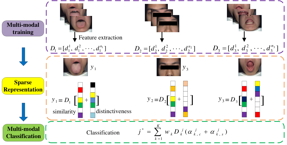
As mentioned above, different modal or feature vectors from a same sample may share some similarity. It is reasonable to assume that representation coefficients coded on their associated dictionaries of different modalities should be similar which would make the representation stable. For example, a test sample, containing tongue modality, facial modality and sublingual modality, is represented as a linear combination of the training samples; since all tasks are belonging to a same sample, they will be well represented by the training samples of their corresponding class, and hence the position and values of significant coefficients are similar. To achieve the above goal, we use [7] the following term to achieve the similarity of different modalities .

where $\bm{\alpha}_{k}$ is the representation coefficient of the $k$-$th$ modality and $\bar{\bm{\alpha}}=\frac{1}{K}\sum_{k=1}^{K}\bm{\alpha}_{k}$ is the mean vector of all $\bm{\alpha}_{k}$ ($K$ is the number of different types of modalities). It is easy to see that Eq. (7) aims to reduce the variance of different representation coefficients $\bm{\alpha}_{k}$, making them similar to each one. However, this assumption is too restrictive since there is also distinctiveness among them. Therefore, it is necessary to not only exploit the similarity among all tasks but also keep the flexibility of each task. In this case, the balance between similarity and distinctiveness among all tasks will represent the original sample more stable and accurate which is beneficial for classification.

To address aforementioned problem, we divide the representation coefficients $\bm{\alpha}_{k}$ into two parts: the similar part and the modal-specific part. Specifically, $\bm{\alpha}_{k}=\bm{\alpha}_{k}^{c}+\bm{\alpha}_{k}^{s}$, where $\bm{\alpha}_{k}^{c}$ denotes the similarity, while $\bm{\alpha}_{k}^{s}$ denotes the distinctiveness. The framework of our proposed method is shown in Fig. 3. The formulation of our model is

where $\mathbf{y}_{k}$ is the test sample, $\mathbf{D}_{k}=[\mathbf{D}_{k}^{1},\mathbf{D}_{k}^{2},\cdot,\cdot,\cdot,\mathbf{D}_{k}^{J}]$ is training samples of the $k$-$th$ task, and $\mathbf{D}_{k}^{i}\in\mathbb{R}^{m_{k}\times n_{k}^{i}}$ is the training set of the $k$-$th$ task of the $i$-$th$ class with $m_{k}$ dimension and $n_{k}^{i}$ samples; $\bar{\bm{\alpha}}^{c}=\frac{1}{K}\sum_{k=1}^{K}\bm{\alpha}_{k}^{c}$ is the mean value of similar sparse representation coefficients of all tasks, and $\tau$ and $\lambda$ are the non-negative penalty constants. From Eq. (8), we can see that our model aims to extract the similar components of each task through $\mathbf{x}_{k}^{c}$, while also keeps individual components of each task through $\mathbf{x}_{k}^{s}$. Note that at the step of exploiting correlation, we do not directly set each $\bm{\alpha}_{k}^{c}$ to be equal, but instead of minimizing the distance between them. This way also makes our approach more flexible. In addition, consider the test sample would be linearly represented by atoms of the dictionary belonging to its own class, we apply $l_{1}$ norm on both $\bm{\alpha}_{k}^{c}$ and $\bm{\alpha}_{k}^{s}$.

We alternatively update the similar coefficients $\bm{\alpha}_{k}^{c}$ and special coefficient $\bm{\alpha}_{k}^{s}$. For example, we update $\bm{\alpha}_{k}^{c}$ by fixing $\bm{\alpha}_{k}^{s}$, and vice versa.

Update $\bm{\alpha}_{k}^{c}$: By fixing $\bm{\alpha}_{k}^{s}$, the optimization solution of Eq. (8) with respect to $\bm{\alpha}_{k}^{c}$ equals to the following problem

we apply Augmented Lagrangian method (ALM) algorithm to modify Eq. (9).

Applying the ALM, the problem of (9) can be modified as follows.

where ${\bm{\alpha}_{k}^{c}}^{\prime}$ is the relaxed variable, $\mathbf{z}_{k}$ is the $k$-$th$ lagrangian multiplier, and $\mu$ is the step value. Then we can optimize $\bm{\alpha}_{k}^{c}$ and ${\bm{\alpha}_{k}^{c}}^{\prime}$ alternatively.

(a) Firstly, we fix ${\bm{\alpha}_{k}^{c}}^{\prime}$ to get ${\bm{\alpha}_{k}^{c}}$

Follow the Ref. [7], a closed-form solution of $\bm{\alpha}_{k}^{c}$ can be derived:

where $\mathbf{P}_{k}=(\mathbf{D}_{k}^{T}\mathbf{D}_{k}+(\tau+\frac{\mu}{2})\mathbf{I})^{-1}$, $\bm{\alpha}_{0,k}^{c}=\mathbf{P}_{k}(\mathbf{D}_{k}^{T}(\mathbf{y}_{k}-\mathbf{D}_{k}\bm{\alpha}_{k}^{s})+\frac{\mu}{2}\bm{\alpha}_{k}^{c^{\prime}}-\frac{\mathbf{z}_{k}}{2})$, and $\mathbf{Q}=(\mathbf{I}-\frac{\tau}{K}\sum_{\eta=1}^{K}\mathbf{P}_{\eta})^{-1}$.

(b) Secondly, after fixing ${\bm{\alpha}_{k}^{c}}$, the optimization solution of Eq. (10) can be reduced to Eq. (13) at the step of updating ${\bm{\alpha}_{k}^{c}}^{\prime}$.

Then ${\bm{\alpha}_{k}^{c}}^{\prime}$ could be derived by operating $\mathrm{Threshold}(\bm{\alpha}_{k}^{c}+\frac{\mathbf{z}_{k}}{\mu},\frac{\lambda}{\mu})$. The operation of soft threshold is shown as follows.

where $\bm{\beta}_{i}$ means the value of the $i$-$th$ component of $\bm{\beta}$. After getting $\bm{\alpha}_{k}^{c}$ and ${\bm{\alpha}_{k}^{c}}^{\prime}$, $\mathbf{z}_{k}$ and $\mu$ can be updated following $\mathbf{z}_{k}=\mathbf{z}_{k}+\mu(\bm{\alpha}_{k}^{c}-{\bm{\alpha}_{k}^{c}}^{\prime})$ and $\mu=1.2\mu$.

Update $\bm{\alpha}_{k}^{s}$: After acquiring ${\bm{\alpha}_{k}^{c}}$, the optimization of Eq. (9) can be reformulated to Eq. (15) at the step of updating $\bm{\alpha}_{k}^{s}$.

In fact, there are many methods to tackle the problem (13). For example, both ALM and Iterative Projection Method (IPM) [9] could deal with it. In this paper, we use IPM to address Eq. (13), as described in Algorithm 1.

The complete algorithm of MMSSL is summarized in Algorithm 2. Note that, since we introduce a new variable $\bm{\alpha}_{k}^{c^{\prime}}$ at the step of updating $\bm{\alpha}_{k}^{c}$, another reasonable way is that we could alternatively update $\bm{\alpha}_{k}^{c^{\prime}}$ and $\bm{\alpha}_{k}^{c}$ until convergence, and then get the solution of $\bm{\alpha}_{k}^{c}$. At this time, the value of $\bm{\alpha}_{k}^{c}$ and $\bm{\alpha}_{k}^{c^{\prime}}$ is similar.

After obtaining the representation coefficients, the decision is ruled in favor of the class with total lowest reconstruction residual over all $K$ tasks.

where $\mathbf{D}_{k,j}$, $\bm{\alpha}_{k,j}^{c}$ and $\bm{\alpha}_{k,j}^{s}$ are the elements of the dictionary $\mathbf{D}_{k}$, the similar coefficient $\bm{\alpha}_{k}^{c}$ and the specific coefficient $\bm{\alpha}_{k}^{j}$ of $j$-$th$ category, respectively; $w_{k}$ is the weight value corresponding to the $k$-$th$ task, which could be obtained by exploiting the method mentioned in [8].

The tongue, facial and sublingual sample database comprises 434 samples split into 192 Healthy samples, 198 DM samples and 114 IGR samples. Each sample has three different modal images including tongue image, facial image and sublingual image, respectively. All images were captured at the Guangdong Provincial TCM Hospital, Guangdong, China, from the early 2014 to the late 2015. Healthy samples were verified through a blood test and other examination. If indicators from these tests fall within a certain range (set by the Guangdong Provincial TCM Hospital), they were regarded as healthy. The FPG test was applied to diagnose whether a sample was suffering from the DM or IGR. When using the FPG test, all the samples had gone at least 12 hours without taking any food. For the DM patients, the blood glucose level was equal or larger than 7.11mmol/L, while the blood glucose level of IGR samples was between 6.1mmol/L and 7.11mmol/L. All these standard indictors are decided by the Guangdong Provincial TCM Hospital.

We first test the performance of our proposed multi-modal classification method in identification of DM for healthy controls, with the tongue, facial and sublingual tasks. We randomly select the number of training samples from 30 to 100, and the rest samples are used for testing. Fig. 4 illustrates the experimental results of our MMSSL approach, compared with the strategies using each individual modality with different classifiers. Note that Fig. 4 only shows the averaged results of 5 independent experiments. It is easy to see that the combined measurements of tongue, facial and sublingual features consistently achieve more accurate discrimination between DM patients and healthy controls. Particularly, compared with single tongue modal feature, our method MMSSL achieves about more than 15% accuracy. The classification accuracies obtained MMSSL are gradually rising with the increasing number of training samples, and they are all higher than 80%. In contrast, the best accuracy on face based modality is only close to 80%.

In addition, Fig. 5 further plots the ROC curves of different classification methods for DM detection when the number of training samples is 70. Note that we only show the ROC curves of SRC and GSRC methods with the single modality to compare with our approach. As the output of SRC and GSRC is reconstruction errors. We use the ratio of different classes to represent the percentage. From Fig. 5, we can see that the area covered by MMSSL based ROC curve is obviously larger than other methods and modalities based curves.

Besides, we also illustrate the maximal and minimal classification rate in 5 independent experiments in Table 1. Note that we only make a comparison between MMSSL and the best performance on the single modality (face modality in this experiment). As we can observe from Table 1, the maximal and minimal rates increase with the increasing number of training samples. Compared with other methods, our proposed methods have a visible improvement both in maximal and minimal accuracies. Specially, when the number of the training samples reaches 100, the discrimination of maximization and minimization obtained by MMSSL achieve 89.01% and 84.29% respectively, while the best values acquired by other approaches are only 83.77% and 75.39%.

Some exemplar results of classification on DM and Healthy are shown in Fig. 6 (the corresponding exemplar results of SRC are shown in Fig. 1). As expected, SVM, SRC and GSRC are capable of discriminating healthy samples using tongue images, but fail to detect DM patients at many times. In contrast, SRC and GSRC have a prominent result on classifying DM using facial images, but fail to detect healthy samples. Different from aforementioned methods using an individual modality, our presented approach get an accurate result of each sample by jointly taking tongue, face and sublingual into account.

In this subsection, we then apply our proposed multi-modal classification method in identification of IGR for healthy controls, with the tongue, facial and sublingual tasks, and make a comparison between MMSSL and other existing methods. Similar with the experiment on DM detection, the number of training samples from 30 to 70 are randomly selected with 5 times, and the rest samples are used for testing. Fig. 7 illustrates the averaged experimental results of our MMSSL approach, compared with the strategies using each individual modality with different classifiers. Our presented multi-modal classification strategy accomplishes a prominent rise in classification accuracy compared with other methods based on tongue, facial or sublingual features. For comparison with SVM, SRC and GSRC on sublingual features, the proposed method also get a slight enhancement in the averaged accuracy. Specially, the rate arrives at 76.68% after combination with tongue, facial and sublingual tasks, while SVM with the sublingual task, which obtains the best result in all individual modalities, only performs 75.87%.

The ROC curves of different classification methods for IGR diagnosis when the number of training samples reaches 70 is plotted in Fig. 8. Similarly, we only show the ROC curves of SRC and GSRC methods with the single modality to compare with our approach. The ROC curves demonstrate that the MMSSL has further performance compared with SRC (tongue), GSRC (tongue) and SRC(sublingual). Additionally, there is a slight improvement acquired by the MMSSL than that of GSRC (sublingual), GSRC (face) and SRC (face).

Table 2 illustrates the maximal and minimal classification rates in 5 independent experiments for IGR diagnosis. Similarly, only a comparison between MMSSL and the best performance on the single modality (sublingual modality in this experiment) is shown. Although at some times SVM have a better result than ours, our method carries out the best values of both maximization and minimization in most conditions. When the number of training samples is 70, the accurate discrimination is 81.44% which is a slightly higher than that of SVM whose value is 79.64%.

References

- [1] World Health Organization, Prevention of blindness from diabetes mellitus,World Health Organization, 2006.
- [2] Wang X, Zhang B, Yang Z, et al, Statistical analysis of tongue images for feature extraction and diagnostics,Image Processing, IEEE Transactions on, 2013, 22(12): 5336-5347.
- [3] Zhang B, Kumar B V K, Zhang D, Noninvasive diabetes mellitus detection using facial block color with a sparse representation classifier, Biomedical Engineering, IEEE Transactions on, 2014, 61(4): 1027-1033.
- [4] Wright J, Yang A Y, Ganesh A, et al, Robust face recognition via sparse representation,Pattern Analysis and Machine Intelligence, IEEE Transactions on, 2009, 31(2): 210-227.
- [5] Zhang B, Kumar B V K, Zhang D, Detecting diabetes mellitus and nonproliferative diabetic retinopathy using tongue color, texture, and geometry features,Biomedical Engineering, IEEE Transactions on, 2014, 61(2): 491-501.
- [6] Lin Z, Chen M, Ma Y, The augmented lagrange multiplier method for exact recovery of corrupted low-rank matrices,arXiv preprint arXiv:1009.5055, 2010.
- [7] Yang M, Zhang L, Zhang D, et al, Relaxed collaborative representation for pattern classification,Computer Vision and Pattern Recognition (CVPR), 2012 IEEE Conference on. IEEE, 2012: 2224-2231.
- [8] Yuan X T, Liu X, Yan S, Visual classification with multitask joint sparse representation,Image Processing, IEEE Transactions on, 2012, 21(10): 4349-4360.
- [9] Rosasco L, Verri A, Santoro M, et al, Iterative projection methods for structured sparsity regularization,2009.
- [10] Shu T, Zhang B, Non-invasive Health Status Detection System Using Gabor Filters Based on Facial Block Texture Features,Journal of medical systems, 2015, 39(4): 1-8.
- [11] Pang B, Zhang D, Li N, et al, Computerized tongue diagnosis based on Bayesian networks,Biomedical Engineering, IEEE Transactions on, 2004, 51(10): 1803-1810.
- [12] Zhang D, Pang B, Li N, et al, Computerized diagnosis from tongue appearance using quantitative feature classification,The American Journal of Chinese Medicine, 2005, 33(06): 859-866.
- [13] Zhang Y, Liang R, Wang Z, et al, Analysis of the color characteristics of tongue digital images from 884 physical examination cases,Journal of Beijing University of Traditional Chinese Medicine, 2005, 28(001): 73-75.
- [14] Su W, Xu Z, Wang Z, et al, Objectified study on tongue images of patients with lung cancer of different syndromes,Chinese Journal of Integrative Medicine, 2011, 17: 272-276.
- [15] Huang B, Wu J, Zhang D, et al, Tongue shape classification by geometric features,Information Sciences, 2010, 180(2): 312-324.
- [16] Li B, Huang Q, Lu Y, et al, A method of classifying tongue colors for traditional chinese medicine diagnosis based on the CIELAB color space,Medical Biometrics. Springer Berlin Heidelberg, 2008: 153-159.
- [17] Li C H, Yuen P C, Tongue image matching using color content,Pattern Recognition,2002, 35(2): 407-419.
- [18] Kim B, Lee S, Cho D, et al, A proposal of heart diseases diagnosis method using analysis of face color,Advanced Language Processing and Web Information Technology, 2008. ALPIT’08. International Conference on. IEEE, 2008: 220-225.
- [19] Liu M, Guo Z, Hepatitis diagnosis using facial color image,Medical Biometrics. Springer Berlin Heidelberg, 2008: 160-167.
- [20] Wang X, Zhang D, An optimized tongue image color correction scheme,Information Technology in Biomedicine, IEEE Transactions on, 2010, 14(6): 1355-1364.
- [21] Maciocia G, The foundations of Chinese medicine,Churchill Livingstone, 1989.
- [22] Zhang H Z, Wang K Q, Jin X S, et al, SVR based color calibration for tongue image,Machine Learning and Cybernetics, 2005. Proceedings of 2005 International Conference on. IEEE, 2005, 8: 5065-5070.
- [23] Zhang B, Wang X, Karray F, et al, Computerized facial diagnosis using both color and texture features,Information Sciences, 2013, 221: 49-59.
- [24] Lin Z, Liu R, Su Z, Linearized alternating direction method with adaptive penalty for low-rank representation,Advances in neural information processing systems. 2011: 612-620.
- [25] Chiu C C, Lan C Y, Chang Y H, Objective assessment of blood stasis using computerized inspection of sublingual veins,Computer methods and programs in biomedicine, 2002, 69(1): 1-12.
- [26] Bengio S, Pereira F, Singer Y, et al, Group sparse coding,Advances in neural information processing systems. 2009: 82-89.
- [27] Hsieh C J, Chang K W, Lin C J, et al, A dual coordinate descent method for large-scale linear SVM,Proceedings of the 25th international conference on Machine learning. ACM, 2008: 408-415.
- [28] Fan R E, Chang K W, Hsieh C J, et al, LIBLINEAR: A library for large linear classification,The Journal of Machine Learning Research, 2008, 9: 1871-1874.
- [29] Cover T M, Hart P E, Nearest neighbor pattern classification,Information Theory, IEEE Transactions on, 1967, 13(1): 21-27.
- [30] Wang X, Zhang B, Guo Z, et al, Facial image medical analysis system using quantitative chromatic feature,Expert Systems with Applications, 2013, 40(9): 3738-3746.