Subparsec-scale dynamics of a dusty gas disk exposed to anisotropic AGN radiation with frequency-dependent radiative transfer

As shown in Fig. 1, we consider a dusty gas disk of radius $\approx 1\;\mathrm{pc}$ around a SMBH of mass $10^{7}\;\mathrm{M_{\odot}}$. We assume that the gas disk is axisymmetric and its symmetric axis is parallel with that of the accretion disk (AD). The inner and outer radii of the disk are assumed to be $0.075\;\mathrm{pc}(\approx R^{\mathrm{iso}}_{\mathrm{sub}})$ and $1\;\mathrm{pc}(\approx 8R^{\mathrm{iso}}_{\mathrm{sub}})$, respectively. We assume that the disk is initially in the hydrostatic equilibrium in the vertical direction (i.e., $z$-direction in Fig. 1) with external gravity due to the SMBH and host galaxy and it rotates with velocities so that the centrifugal force balances with the external gravity. The hydrogen number density at the mid-plane, $n_{\mathrm{mid}}(\mathrm{H})$, is constant over galactic radii and is assumed to be $n_{\mathrm{mid}}(\mathrm{H})=10^{7}\;\mathrm{cm^{-3}}$, which is intermediate between number densities of narrow-line region (NLR) and BLR. Thus, our choice of gas density is reasonable. In this study, we consider the RHD evolution of this gas disk when irradiated by an AGN with bolometric luminosity $L_{\mathrm{bol}}=10^{45}\;\mathrm{erg\;s^{-1}}$. The corresponding Eddington ratio is $\approx 0.77$ and it is higher than typical Eddington ratio of radiative-mode AGNs ($\sim 0.1$). The reason for this choice is because studying AGNs with high accretion rates is more important than those with low accretion rates in terms of AGN feedback.

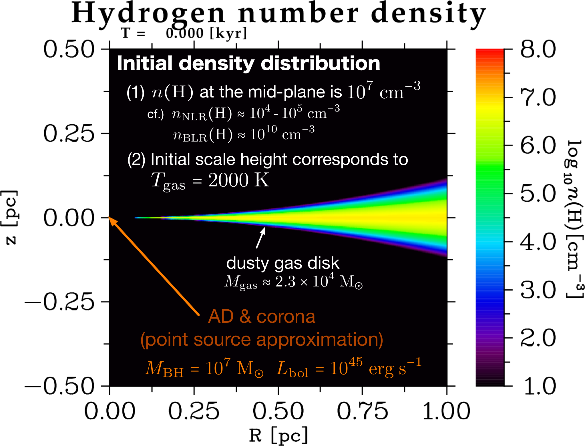
We assume that radiation from AGN is emitted by the AD and the corona (e.g., Kawaguchi et al. 2001), which are located at the origin in Fig. 1. Following previous studies (Netzer 1987; Kawaguchi & Mori 2010; Kawaguchi & Mori 2011; Liu & Zhang 2011), we assume that the AD radiates anisotropically due to the change in the apparent surface area with the line-of-sight (LOS) and the limb darkening effect. In this case, the monochromatic radiation flux of the AD is given by

where $\theta$ is the angle measured from the symmetric axis of the AD, $L^{\mathrm{AD}}_{\nu}$ is the monochromatic luminosity of the AD, and $\tau_{\nu}$ is the optical depth. On the other hand, we assume that the corona emits radiation isotropically and its monochromatic radiation flux is simply given by $F^{\mathrm{corona}}_{\nu}=L^{\mathrm{corona}}_{\nu}\exp(-\tau_{\nu})/(4\pi r^{2})$. The fraction of luminosity of the corona is controlled by the parameter $f_{\mathrm{X}}\equiv L_{\mathrm{corona}}/L_{\mathrm{bol}}$ and the fiducial value in this study is $0.08$. A detailed description of SEDs of both components is given in § 2.2.

We assume that the external gravitational potential consists of a SMBH, a nuclear star cluster (NSC), and a nuclear stellar disk (NSD). All of these are modeled by the Plummer potential $\Phi=-GM/\sqrt{r^{2}+b^{2}}$ (Plummer 1911). The parameters adopted are as follows: $M_{\mathrm{BH}}=10^{7}\;\mathrm{M_{\odot}}$, $b_{\mathrm{BH}}=0.1\;\mathrm{pc}$, $M_{\mathrm{NSC}}=10^{8}\;\mathrm{M_{\odot}}$, $b_{\mathrm{NSC}}=10\;\mathrm{pc}$, $M_{\mathrm{NSD}}=10^{9}\;\mathrm{M_{\odot}}$, and $b_{\mathrm{NSD}}=100\;\mathrm{pc}$. Note that a large value for $b_{\mathrm{BH}}$ is intended to avoid a very small timestep near the origin and hence numerical results near the origin are not reliable.

The numerical simulation is started when the AGN is turned on and we numerically follow the subsequent evolution of the disk. In order to take into account the five important effects described in § 1 (➊-➎), we perform hydrodynamic simulations taking into account (1) photoionization and photodissociation of gas, (2) radiative transfer (RT) of IR photons reemitted by heated dust grains, (3) radiation pressure on gas and dust, and (4) self-gravity of gas. The rates of photoionization, photodissociation, photoelectric heating and so on are evaluated by performing RT calculations of direct radiation from AD and corona. The resultant rates are then used to calculate non-equilibrium chemical reactions of the following chemical species: $\mathrm{e^{-}}$, $\mathrm{H^{+}}$, $\mathrm{H^{0}}$, $\mathrm{H^{-}}$, $\mathrm{H_{2}}$, $\mathrm{H^{+}_{2}}$, $\mathrm{He^{0}}$, $\mathrm{He^{+}}$, $\mathrm{He^{++}}$, and dust. The effects of metal is considered in an approximate way. We take into account Compton heating/cooling in a simplest way as well as standard cooling processes pertaining to hydrogen, helium, and dust (see § 2.3 and § 3.2). As shown later, a dusty outflow is launched from the disk surface heated strongly by X-ray/UV/optical photons emitted by the AD and the corona. We measure this outflow rate. X-ray photons also heat the whole of the disk almost uniformly and determine the gas pressure in the interior of the disk. We investigate how the structures of density and temperature of the disk are determined by X-ray heating and radiation pressure of IR photons. Thus, various physical processes should play roles in shaping the gas structure and the gas flow. In this study, we devote ourself clarifying the effects of each process. To this end, we perform a number of simulations with switching some process(es) on and off and with fixing the parameters that characterize the system such as $M_{\mathrm{BH}}$, $L_{\mathrm{bol}}$, and $n_{\mathrm{mid}}(\mathrm{H})$. The dependency on these parameters will be examined elsewhere.

Table 1 summarize the simulation runs and their names show which physical processes are switched on or off in the simulations. Comparing different runs enables us to clarify the effects of each physical process on the structures of density, temperature, and gas flow and the outflow rate. For instance, we can discriminate the effects of the radiation pressure of IR photons by the comparison between gra01_wo_sca and gra01_wo_sca_noRP-IR. More detail for each run is described when we explain our numerical results (§ 4).

The SED of AD is modeled by the SED model given by Nenkova et al. (2008a) except for models whose name contain the word _S05, for which we use the SED model given by Schartmann et al. (2005) to check the effects of SED shape (for the detail of SED shape, see the original papers or § 2.2 in Namekata et al. 2014).

The SED of corona is modeled by a broken power-law (BPL):

where $\lambda_{\mathrm{b}}=0.144762\;\mathrm{\AA}$, $\lambda_{\mathrm{h}}=30\;\mathrm{\AA}$, and $\Delta\lambda_{\mathrm{co}}=30\;\mathrm{\AA}$. The parameter values are determined so that the the BPL resembles in shape to tableAGN, which is a SED model for AGN implemented in the Cloudy (Ferland et al. 2013). The shapes and properties of the AGN SEDs adopted in this study are shown in Fig. 2 and Table 2, respectively. The range of wavelength considered in this study is $\lambda=0.01\operatorname{-}10^{7}\mathrm{\AA}$, which are denoted by $[\lambda_{\min},\lambda_{\max}]$ (the corresponding frequency range is $[\nu_{\min},\nu_{\max}]$).

We assume that an ISM consists of chemical species of $\mathrm{e^{-}}$, $\mathrm{H^{+}}$, $\mathrm{H^{0}}$, $\mathrm{H^{-}}$, $\mathrm{H_{2}}$, $\mathrm{H^{+}_{2}}$, $\mathrm{He^{0}}$, $\mathrm{He^{+}}$, $\mathrm{He^{++}}$, dust, and metals and assume the tight dynamical coupling between gas and dust. We solve chemical reactions for all the species except for metal, whose effects are taken into account only through a cooling function (described later). The chemical reactions and radiative and thermal processes adopted in this study are taken from previous studies (e.g., Shapiro & Kang 1987; Abel et al. 1997; Glover & Brand 2003; Yoshida et al. 2006; Glover & Abel 2008) and are summarized in Tables 6 and 3, respectively. The reaction coefficients for a few reactions are updated (see Appendix A).

As in Namekata et al. (2014), we compute the internal energy density of gas, $e_{\mathrm{th}}$, by the equation

where $p_{\mathrm{th}}$ is the thermal pressure and $\gamma_{\mathrm{eff}}$ is the effective specific heat ratio of gas, which is defined as

where $X_{k}$ and $\gamma_{k}$ are the number fraction and the specific heat ratio of species $k$, respectively. We assume $\gamma_{k}=5/3$ except for molecular hydrogen for which we use the formula given by Landau & Lifshitz (1980) (see also Yoshida et al. 2006).

We assume that dust consists of graphite whose mass density is $2.26\;\mathrm{g\;cm^{-3}}$ (Laor & Draine 1993), because SED modelings of AGNs suggest the presence of hot graphite dust near the dust sublimation radius (Mor & Netzer 2012). We do not consider size distribution and assume that the grain radius is $a_{\mathrm{gr}}=0.1\;\micron$ for most of our models. The dust-to-gas mass ratio is assumed to be $0.01$. The optical constants such as the absorption efficiency $\mathcal{Q}_{\mathrm{abs}}(\nu,a_{\mathrm{gr}})$ and the scattering efficiency $\mathcal{Q}_{\mathrm{sca}}(\nu,a_{\mathrm{gr}})$ are calculated by the photoionization code Cloudy (version C13.03, last described by Ferland et al. 2013) and are essentially the same as those in Laor & Draine (1993). The temperature of dust grain, $T_{\mathrm{gr}}$, is determined assuming thermal equilibrium:

where $r$ is the distance from AGN, $L_{\nu}(\theta)$ is the monochromatic luminosity of AGN, $\tau_{\nu}$ is the optical depth, $n_{\mathrm{gr}}$ is the number density of grain, $\Omega$ is the solid angle, $I^{\mathrm{IR}}_{\nu}(\Omega)$ is the intensity of IR photons, $B_{\nu}$ is the Planck function, and $\Lambda_{\mathrm{g\operatorname{-}gr}}$ is the rate of energy transfer due to gas-dust collision (Burke & Hollenbach 1983; we assume the average accommodation coefficient $\overline{\alpha}_{T}=0.4$ [see Namekata et al. 2014]). In this study, we assume that the sublimation temperature of dust grain is $T_{\mathrm{sub}}=1800\;\mathrm{K}$. Sublimation and solidification of dust are treated as follows:

• •

  dust grain evaporates instantaneously if $T_{\mathrm{gr}}>T_{\mathrm{sub}}$.

• •

  the vapor of dust grain becomes solidified instantly if (i) $T_{\mathrm{gas}}<T_{\mathrm{sub}}$ and (ii) $T_{\mathrm{gr}}$ is smaller than $T_{\mathrm{sub}}$ after the solidification.

The destruction of dust grains due to thermal sputtering is considered in model gra01_wo_sca_Tts10^6K_SG only.

The effects of metals are taken into account in the form of cooling function, because it is numerically too costly to perform long-term RHD simulations with taking all of important chemical reactions relevant to metals into consideration even for a modern super computer. The cooling function is calculated by the Cloudy assuming the metallicity of ISM is solar. Figure 3 shows the resultant cooling function. We approximate metal cooling, $\Lambda_{\mathrm{metal}}$, by this cooling function, although the simultaneous use of $\Lambda_{\mathrm{metal}}$ and the radiative processes listed in Table 3 results in double counts of some of cooling processes such as $\mathrm{H_{2}}$ cooling. This approximation is justified by the following additional measures:

1. 1.

   The cooling function is applied only for low temperature ($T_{\mathrm{gas}}\lesssim 10^{4}\;\mathrm{K}$) gas where gas density is generally high and the ionization parameter is low (see § 4). In such regions, metal cooling (e.g., [O i]$63\micron$, [C ii]$157\micron$, emission lines from CO and $\mathrm{H_{2}O}$ molecules) is expected to dominate other coolings due to hydrogen and helium. Hence, the above approximation can be acceptable as a zeroth order approximation. To restrict the metal cooling to low temperature gas, $\Lambda_{\mathrm{metal}}$ is computed by

   $$\Lambda_{\mathrm{metal}}(n({\mathrm{H}}),T_{\mathrm{gas}})=\Lambda(n({\mathrm{H}}),T_{\mathrm{gas}})\exp\left[-\left(\dfrac{T_{\mathrm{gas}}}{15000}\right)^{8}\right],$$

   (7)

   where $\Lambda(n({\mathrm{H}}),T_{\mathrm{gas}})$ is the cooling function computed by the Cloudy. As noted above, the use of $\Lambda_{\mathrm{metal}}$ causes the double counts of some cooling processes. This property is, however, useful to place a lower limit on the scale height of gas disk.

2. 2.

   For regions with $T_{\mathrm{gas}}\gtrsim 10^{4}\;\mathrm{K}$, metal cooling is not applied. This is justified because high temperature is realized in the outflow region (see § 4) where the ionization parameter is extremely high and recombination cooling by metal will be suppressed due to overionization⁶⁶ 6 Thoul & Weinberg (1996) have shown that a strong UV background radiation smooths out the peaks of the cooling function at $T_{\mathrm{gas}}=10^{4}\operatorname{-}10^{5}\;\mathrm{K}$, whose origin are recombination coolings due to hydrogen and helium (see their Fig.1). Similarly, it is expected that recombination coolings due to metals disappear in regions with large ionization parameters.. Actually, a photoionization calculation by the Cloudy predicts that the gas temperature in the outflow region is completely determined by the balance between Compton heating and Compton cooling and recombination coolings due to metals are negligible.

For the ISM model described above, we compute the equilibrium temperatures of gas and dust at a distance of $r=0.5\;\mathrm{pc}$ from an AGN with $L_{\mathrm{bol}}=5\times 10^{44}\;\mathrm{erg\;s^{-1}}$ and the result is shown in Fig. 4. It is clear from the figure that ISM can become four-phases: very hot ($T_{\mathrm{gas}}\approx T_{\mathrm{comp}}$), hot ($T_{\mathrm{gas}}\approx(1\operatorname{-}2)\times 10^{4}\;\mathrm{K}$), warm ($10^{3}\;\mathrm{K}<T_{\mathrm{gas}}<10^{4}\;\mathrm{K}$), and cold ($T_{\mathrm{gas}}<10^{3}\;\mathrm{K}$) media.

We solve the hydrodynamic part i of the governing equations using the M-AUSMPW⁺ scheme (Kim & Kim 2005a) and the multidimensional limiting process with fifth order interpolation (MLP5, Kim & Kim 2005b). The M-AUSMPW⁺ scheme, as the name implies, is one of the advection upstream splitting method (AUSM) type schemes (Liou & Steffen 1993) and is more robust and less dissipative in multi-dimensional flows than the previous AUSM type schemes such as AUSM⁺ (Liou 1996) and AUSMPW⁺ (Kim et al. 2001), owing to (i) discontinuity detection using Mach number and pressure and (ii) addition of correction step of the primitive variables at the cell interfaces based on the smoothness of the flow. In this study, we do not employ the modification of the pressure splitting function suggested by Kim & Kim (2005a) (see §2.3.2 in their paper), because it results in negative thermal energy in some cases. Combined with MLP5, the M-AUSMPW⁺ scheme achieves fifth-order accurate in space in smooth regions of the flow. For accurate advection of chemical species, we employ the consistent multifluid advection (CMA) method (Plewa & Müller 1999)⁷⁷ 7 When combining the CMA method with the M-AUSMPW⁺ scheme, we need to calculate $\mn@boldsymbol{Y}_{\mathrm{L[R],superbee}}$ which is the chemical abundances at the left and right sides of a cell interface and are obtained by the Monotonic Upstream-Centered Scheme for Conservation Laws (MUSCL) interpolation with the superbee limiter. In a certain situation, abundance of a particular element or all the elements can become zero and $\rho_{\mathrm{L[R],superbee}}=\sum_{k}\rho^{(k)}_{\mathrm{L[R],superbee}}$ does not hold in this case, where $\rho^{(k)}$ is density of species $k$. This happens for a cell interface separating a fully-ionized region and a fully neutral region, for example. In such cases, we simply use the chemical abundance of the nearest cell center as $\mn@boldsymbol{Y}_{\mathrm{L[R],superbee}}$.. This combination is also adopted and tested in Namekata & Habe (2011).

The gravitational force and its power are treated as source terms of the hydrodynamic equations. The self-gravity is computed by the tree method (Barnes & Hut 1986) with modification to treat an axisymmetric system (see Appendix B). The opening angle criterion, $\theta^{\mathrm{grv}}_{\mathrm{crit}}$, is assumed to be 0.35. We take into account the monopole components only and use a quadtree to construct group interaction lists (Barnes 1990; Makino 1991).

The code is parallelized with the Message Passing Interface (MPI). Time integration is performed by the second order total variation diminishing (TVD) Runge-Kutta method (Shu 1988).

We solve the RT parts (ii,iv) of the governing equations using a hybrid method, in which the RT of direct radiation from AD and corona is solved by the (photon-conservative) long-characteristics method (LCM) while we solve that of IR photons by the finite-volume method (FVM). In the RT calculations, the following assumptions are made:

1. (A1)

   The speed of light is infinity.

2. (A2)

   Gas is assumed to be at the rest. Hence, the Poynting-Robertson effect and special relativistic effects such as the Doppler-shift and the radiation drag are neglected.

3. (A3)

   We assume that direct photons singly-scattered by electrons escape from the system without any interactions. In other words, we do not consider multiple electron (Compton) scattering of direct photons.

4. (A4)

   We ignore dust scattering of direct photons.

5. (A5)

   We also neglect electron (Compton) scattering of IR photons.

6. (A6)

   We assume that dust scattering of IR photons is isotropic.

7. (A7)

   We do not perform an exact RT calculation of cooling photons arisen by the cooling processes described in § 2.3. Instead, we assume that these cooling photons are optically-thin in most of the runs, but, in the runs with ‘LDA1‘, their RT effects are approximately taken into account by using the LDA approximation (see § 2.1 and § 4.2).

8. (A8)

   We employ the so-called on-the-spot (OTS) approximation (Osterbrock & Ferland 2006) for recombination photons of the reactions R2, R31, and R32 (see Table 6).

9. (A9)

   We use an approximate formula for the photodissociation rate of $\mathrm{H_{2}}$ due to the two-step Solomon process (Draine & Bertoldi 1996).

Global timestep $\Delta t$ is determined as follows

where we use $(i,j)$ as an identifier of a fluid cell as in the usual manner, $c_{s,ij}$ is the adiabatic sound speed of cell $(i,j)$, and $\mn@boldsymbol{a}^{\mathrm{tot,eff}}_{ij}$ is the sum of gravitational, centrifugal, and radiative accelerations. In this study, we assume $C_{\mathrm{hyd}}=C_{\mathrm{accl}}=0.15$.

An uniform spatial grid is used to cover a computational box with a radius $1.2\;\mathrm{pc}$ and a height $1.2\;\mathrm{pc}$. In most of models, we use $512^{2}$ grid points (the corresponding spatial resolution is $2.34\times 10^{-3}\;\mathrm{pc}$), but, some models are performed with $1024^{2}$ grid points to check the effects of spatial resolution. As for the discretization of solid angle, we assume $N_{\phi}=N_{\theta}=12$ (see Appendix D).

The initial density distribution of a dusty gas disk is obtained by solving the isothermal hydrostatic equation

where $a^{\mathrm{grv,ext}}_{z}$ is the $z$ component of the acceleration of external gravity, $c_{s}$ is the adiabatic sound speed of gas. The outer edge of the disk $R_{\mathrm{out}}$ is smoothed by multiplying the density at $R>R_{\mathrm{out}}$ by a factor of $\exp\left[-20\frac{R-R_{\mathrm{out}}}{R_{\mathrm{out}}}\right]$, where we assume $R_{\mathrm{out}}=1\;\mathrm{pc}$ as described in § 2.1. We assume that the disk initially consists of a neutral atomic gas ($Y(\mathrm{H^{0}})=0.748125$, $Y(\mathrm{He^{0}})=0.251875$, $Y(k)=0$; where $Y(\cdot)$ is mass abundance and $k$ denotes chemical species other than $\mathrm{H^{0}}$ and $\mathrm{He^{0}}$) and the gas and dust temperatures are uniform in the disk with values of $T_{\mathrm{gas}}=2000\;\mathrm{K}$ and $T_{\mathrm{gr}}=100\;\mathrm{K}$. The initial velocity field is $\mn@boldsymbol{v}=\left(0,\sqrt{R|a^{\mathrm{grv,ext}}_{R}|},0\right)$, where $a^{\mathrm{grv,ext}}_{R}$ is the $R$ component of the acceleration of external gravity.

All the boundary conditions are fixed boundaries. Around the symmetric axis, we set up a boundary zone where deviations of primitive variables from the initial values and pressure fluctuation are artificially damped. This boundary zone is introduced to prevent negative density or negative internal energy at extremely low density regions that are formed near the symmetric axis due to strong radiation pressure from AGN. For details, see Appendix C.

Figures 7 and 8 show the time evolution of density, gas and dust temperatures in the reference models. Immediately after the simulations are started, the surface layer of the initial gas disk is strongly heated by absorption of ionizing photons from AGN and an dusty outflow is launched from the disk surface. Hard X-ray photons from corona quickly rise the gas temperature of the outflowing gas and it eventually settles at Compton temperature ($\approx 10^{7}\;\mathrm{K}$). Thus, the gas temperature is determined by the balance between Compton heating and Compton cooling (readers may have noticed that the gas temperature is large enough that small dust grains are rapidly destroyed by thermal sputtering. The effects of thermal sputtering is examined in § 4.5). Thermal pressure in the outflowing gas also increases and, as a result, the outflowing gas thermally expands in a vertical direction (its sound speed is comparable to circular velocity). At the same time, the outflow is strongly accelerated in the radial direction by dust absorption and electron scattering. This competition determines a scale height of the outflowing gas. The hydrogen number density of the outflow is $n({\mathrm{H}})\approx 10^{2\operatorname{-}3}\;\mathrm{cm^{-3}}$ and the outflow velocity increases from $\sim 100\;\mathrm{km\;s^{-1}}$ directly above the disk surface to $(2\operatorname{-}3)\times 10^{3}\;\mathrm{km\;s^{-1}}$ at the outer layer of the outflow (Fig. 9). The hydrogen column density of the outflow region is $N_{\mathrm{H}}\lesssim 2\times 10^{21}\;\mathrm{cm^{-2}}$ (Fig. 10), and hence, the outflow within $R<1\;\mathrm{pc}$ cannot be regard as an obscuring torus ($N_{\mathrm{H}}>3\times 10^{21}\;\mathrm{cm^{-2}}$ is required to suppress broad UV lines according to Hasinger 2008). The dust temperature in the outflow region is mainly determined by the balance between photoheating and cooling due to thermal emission and is $T_{\mathrm{gr}}\approx 500\operatorname{-}10^{3}\;\mathrm{K}$ (Figs. 7i-l and 8i-l).

In the absence of metal cooling, the system reaches a quasi-steady state by $t=2\;\mathrm{kyr}$, which consists of a nearly neutral, dense ($n({\mathrm{H}})\approx 10^{6\operatorname{-}8}\;\mathrm{cm^{-3}}$), thin ($h/r\approx 0.06$) disk and the dusty wind described above (Fig. 7b-d). X-ray heating determines the thermal state of the neutral thin disk and the gas and dust temperatures are $\approx(1\operatorname{-}3)\times 10^{4}\;\mathrm{K}$ and $\approx 200\;\mathrm{K}$, respectively (Fig. 7f-h). On the other hand, in the presence of metal cooling, the initial disk begins to collapse in a vertical direction at the start of the simulation and a very thin disk forms at $t\approx 6\;\mathrm{kyr}$ (Fig. 8c,d). After that, the system roughly keeps a quasi-steady state. The hydrogen number density in the thin disk is $10^{7\operatorname{-}9}\;\mathrm{cm^{-3}}$. The gas temperature in the thin disk varies from $\approx 10^{4}\;\mathrm{K}$ at the inner part of the disk to $\approx 100\;\mathrm{K}$ at the outer part of the disk (e.g., Fig. 8g,h), where most of hydrogen takes the form of molecular hydrogen. The true scale height of the neutral disk should be intermediate between the scale heights of both models, because we use a overestimated metal cooling function as described in § 2.3. The inner edge ($R\approx 0.38\operatorname{-}0.56\;\mathrm{pc}$) of the neutral thin disk fragments into a clumpy structure and cloudlets are occasionally blown off likely due to ram pressure and radiation pressure (e.g., Fig. 8d). These cloudlets are promptly destroyed by combination of ram pressure stripping and photoevaporation. In addition, chimney-like structures are frequently formed at the disk surface in the model with metal cooling (Fig. 8c). The time evolution of these inhomogeneous features depends on spatial resolution and we come back to this point in § 4.3.

In order to examine the reasons why the neutral disk is geometrically thin and make clear the contribution of IR photons to the vertical support of the neutral disk, we perform additional five simulations (gra01_wo_sca, gra01_w_sca, gra01_wo_sca_noRP-IR, gra01_wo_sca_noRP-drct, and gra01_wo_sca_noRP-all) and compare them each other. We first check if dust scattering of IR photons, which is neglected in the reference models, changes the structure of the neutral disk, by comparing the result of model gra01_wo_sca with that of model gra01_w_sca. Figs 11(a),(b) show the spatial distributions of hydrogen number density at $t=8.75\;\mathrm{kyr}$ in these two models. As is clear from the figure, there is no difference between them, indicating that dust scattering of IR photons does not affect the disk structure. Next, we compare the result of model gra01_wo_sca with that of model gra01_wo_sca_noRP-IR, in which radiation pressure due to IR photons is switched off, to examine the contribution of IR photons to the vertical support of the disk. The density distributions of both models are shown in Figs 11(a),(c). The disk thickness is almost the same in these two models, suggesting that the vertical support due to IR photons is not effective. This is supported by the comparison between models gra01_wo_sca and gra01_wo_sca_noRP-drct, in the latter of which only radiation pressure due to IR photons is taken into account. Fig. 11(d) shows the density distribution of model gra01_wo_sca_noRP-drct when the total gas mass is $\approx 2.2\times 10^{4}\;\mathrm{M_{\odot}}$. The disk thickness is virtually the same as that of model gra01_wo_sca. Thus, the disk thickness does not depend on the presence or the absence of radiation pressure due to IR photons. However, radiation pressure due to IR photons enhances the outflow rate as shown by the comparison between Figs. 11(a) and (e). The total gas mass at $t=8.75\;\mathrm{kyr}$ in model gra01_wo_sca_noRP-drct is smaller than that in model gra01_wo_sca. Finally, we compare the result of model gra01_wo_sca with that of model gra01_wo_sca_noRP-all, in which all of radiation pressure is switched off, and as a result, the disk thickness is determined only by thermal pressure. Fig. 11(f) show the density distribution at $t=8.75\;\mathrm{kyr}$ in model gra01_wo_sca_noRP-all. The disk thickness in this model is much the same as that in model gra01_wo_sca. From these results, we conclude that the neutral disk is mainly supported by gas pressure, rather than radiation pressure of IR photons.

To make it more clear how radiation pressure due to IR photons acts, we plot the spatial distribution of the ratios of various types of radiative accelerations normalized by the acceleration due to the external gravity in Fig. 13. Fig. 13(a) shows that the outflowing gas is partially supported in the vertical direction by radiation pressure of IR photons reemitted by the neutral disk, while the neutral disk is compressed by IR photons reemitted by the outflowing gas. Thus, IR photons is not effective in supporting the neutral disk. One of other reasons why the neutral disk does not expand vertically is that radiation pressure from direct photons and thermal pressure of the outflowing gas compress or confine the neutral thin disk. This can be confirmed by both Fig. 11 and Figs. 13(c),(d). Figs 11(a),(c), and (e) show that the presence of radiation pressure due to direct photons reduces the decreasing rate of gas mass in the system. Figs 13(c),(d) show that radiation pressure due to direct photons near the surface of the neutral disk is as large as $a^{\mathrm{rad,drct}}_{\mathrm{R}}/|a^{\mathrm{grv,ext}}_{\mathrm{R}}|\approx 10$. Another reason is certainly that $T_{\mathrm{gr}}$ in the neutral disk does not become large enough due to both the anisotropic AD radiation and dust absorption of direct photons in the outflow region.

Figure 14 shows the time evolution of gas mass in the computational box for each model. Mass outflow rate can be estimated from the time derivative. In the absence of metal cooling, the outflow rate are $0.05\operatorname{-}0.1\;\mathrm{M_{\odot}}\;\mathrm{yr}^{-1}$ during $t=2\operatorname{-}6\;\mathrm{kyr}$ depending on the X-ray luminosity fraction. These values correspond to $\approx 20\%\operatorname{-}50\%$ of Eddington mass accretion rate $\dot{M}_{\mathrm{Edd}}$, which is given by

References

- Abel et al. (1997) Abel T., Anninos P., Zhang Y., Norman M. L., 1997, New Astronomy, 2, 181
- Aldrovandi & Péquignot (1973) Aldrovandi S., Péquignot D., 1973, A&A, 25, 137
- Allision & Dalgarno (1969) Allision A., Dalgarno A., 1969, Atomic Data, 1, 91
- Antonucci (1993) Antonucci R., 1993, ARA&A, 31, 473
- Auer (2003) Auer L., 2003, in Hubney I., Mihalas D., Werner K., eds, ASP Conference Series Vol. 288, Stellar Atmosphere Modeling. Astronomical Society of the Pacific, San Francisco, pp 3–15
- Balsara (2001) Balsara D., 2001, J. Quant. Spectrosc. Radiative Transfer, 69, 671
- Barlow (1984) Barlow S., 1984, PhD thesis, University of Colorado, Boulder
- Barnes (1990) Barnes J. E., 1990, Journal of Computational Physics, 87, 161
- Barnes & Hut (1986) Barnes J. E., Hut P., 1986, Nature, 324, 446
- Bates & Öpik (1968) Bates D., Öpik U., 1968, Journal of Physics B: Atomic and Molecular Physics, 1, 543
- Begelman & McKee (1990) Begelman M. C., McKee C. F., 1990, ApJ, 358, 375
- Ben Salah et al. (2004) Ben Salah M., Askri F., Slimi K., Ben Nasrallah S., 2004, International Journal of Heat and Mass Transfer, 47, 2501
- Bentz et al. (2009) Bentz M. C., Peterson B. M., Netzer H., Pogge R. W., Vestergaard M., 2009, ApJ, 697, 160
- Bruls et al. (1999) Bruls J., Vollmöller P., Schüssler M., 1999, A&A, 348, 233
- Burgess & Seaton (1960) Burgess A., Seaton M., 1960, MNRAS, 121, 471
- Burke & Hollenbach (1983) Burke J. R., Hollenbach D., 1983, ApJ, 265, 223
- Busche & Hillier (2000) Busche J. R., Hillier D. J., 2000, ApJ, 531, 1071
- Carlson (1963) Carlson B. G., 1963, in Alder B., Fernbach S., Rotenberg M., eds, Statistical physics, Vol. 1, Methods in computational physics : advances in research and applications. Academic Press, New York
- Carlson & Lathrop (1968) Carlson B. G., Lathrop K., 1968, in Greenspan H., Kelber C. N., Okrent D., eds, , Computing Methods in Reactor Physics. Gordon & Breach Science Publishers Ltd., New York, Chapt. 3, pp 171–266
- Cazaux & Spaans (2004) Cazaux S., Spaans M., 2004, ApJ, 611, 40
- Cazaux & Tielens (2004) Cazaux S., Tielens A., 2004, ApJ, 604, 222
- Cazaux & Tielens (2010) Cazaux S., Tielens A., 2010, ApJ, 715, 698
- Cen (1992) Cen R., 1992, ApJS, 78, 341
- Chai et al. (1994) Chai J. C., Lee H. S., Patankar S. V., 1994, Journal of Thermophysics and Heat Transfer, 8, 419
- Chan & Krolik (2015) Chan C.-H., Krolik J. H., 2015, arXiv:1511.00333v1
- Chibisov et al. (1997) Chibisov M., Brouillard F., Chenu J., Cherkani M., Fussen D., Olamba K., Szücs S., 1997, J.Phys.B: At.Mol.Opt.Phys., 30, 991
- Chui et al. (1992) Chui E., Raithby G., Hughes P., 1992, Journal of Thermophysics and Heat Transfer, 6, 605
- Chung et al. (1993) Chung Y., Lee E.-M., Masuoka T., Samson J. A., 1993, J. Chem. Phys., 99, 885
- Coelho (2008) Coelho P., 2008, J. Quant. Spectrosc. Radiative Transfer, 109, 189
- Coelho (2014) Coelho P. J., 2014, J. Quant. Spectrosc. Radiative Transfer, 143, 3
- Croft et al. (1999) Croft H., Dickinson A., Gadéa F., 1999, MNRAS, 304, 327
- Cullen & Dehnen (2010) Cullen L., Dehnen W., 2010, MNRAS, 408, 669
- Czerny & Hryniewicz (2011) Czerny B., Hryniewicz K., 2011, A&A, 525, L8
- Czerny et al. (2009) Czerny B., Chevallier L., Gonçalves A., Różańska A., Dumont A.-M., 2009, A&A, 499, 349
- Czerny et al. (2015) Czerny B., et al., 2015, Advances in Space Research, 55, 1806
- Dalgarno & Lepp (1987) Dalgarno A., Lepp S., 1987, in Vardya M., Tarafdar S., eds, Astrochemistry, Proceedings of the IAU Symposium No.120. D. Reidel Publishing Co. (Dordrecht), held 3-7 December 1985 in Goa, India, pp 109–118
- Dorodnitsyn & Kallman (2012) Dorodnitsyn A., Kallman T., 2012, ApJ, 761, 70
- Dorodnitsyn et al. (2015) Dorodnitsyn A., Kallman T., Proga D., 2015, arXiv:1512.03854v1
- Dove et al. (1987) Dove J., Rusk A., Cribb P., Martin P., 1987, ApJ, 318, 379
- Draine & Bertoldi (1996) Draine B., Bertoldi F., 1996, ApJ, 468, 269
- Draine & Salpeter (1979) Draine B., Salpeter E., 1979, ApJ, 231, 77
- Dujardin et al. (1987) Dujardin G., Besnard M., Hellner L., Malinovitch Y., 1987, Phys. Rev. A, 35, 5012
- Dullemond & Turolla (2000) Dullemond C., Turolla R., 2000, A&A, 360, 1187
- Dullemond & van Bemmel (2005) Dullemond C., van Bemmel I., 2005, A&A, 436, 47
- Dunn (1968) Dunn G. H., 1968, Physical Review, 172, 1
- Evrard (1988) Evrard A. E., 1988, MNRAS, 235, 911
- Feltre et al. (2012) Feltre A., Hatziminaoglou E., Fritz J., Franceschini A., 2012, MNRAS, 426, 120
- Ferland et al. (1992) Ferland G., Peterson B., Horne K., Welsh W., Nahar S., 1992, ApJ, 387, 95
- Ferland et al. (2013) Ferland G., et al., 2013, Revista Mexicana de Astronomía y Astrofísica, 49, 137
- Fukugita & Kawasaki (1994) Fukugita M., Kawasaki M., 1994, MNRAS, 269, 563
- Galli & Palla (1998) Galli D., Palla F., 1998, A&A, 335, 403
- Glass-Maujean (1986) Glass-Maujean M., 1986, J. Chem. Phys., 85, 4830
- Glass-Maujean (1988) Glass-Maujean M., 1988, J. Chem. Phys., 89, 2839
- Glover (2003) Glover S. C., 2003, ApJ, 584, 331
- Glover & Abel (2008) Glover S., Abel T., 2008, MNRAS, 388, 1627
- Glover & Brand (2003) Glover S., Brand P., 2003, MNRAS, 340, 210
- Godoy & DesJardin (2010) Godoy W. F., DesJardin P. F., 2010, Journal of Computational Physics, 229, 3189
- Gonçalves et al. (2007) Gonçalves A., Collin S., Dumont A.-M., Chevallier L., 2007, A&A, 465, 9
- Greenhill et al. (1995) Greenhill L., Jiang D., Moran J., Reid M., 1995, ApJ, 440, 619
- Hasinger (2008) Hasinger G., 2008, A&A, 490, 905
- Hatzminaoglou et al. (2015) Hatzminaoglou E., Hernán-Caballero A., Feltre A., Ferrer N. P., 2015, ApJ, 803, 110
- Hayek et al. (2010) Hayek W., Asplund M., Carlsson M., Trampedach R., Collet R., Gudiksen B., Hansteen V., Leenaarts J., 2010, A&A, 517, A49
- Heckman & Best (2014) Heckman T. M., Best P. N., 2014, ARA&A, 52, 589
- Herrnstein et al. (2005) Herrnstein J., Moran J., Greenhill L., Trotter A. S., 2005, ApJ, 629, 719
- Hirashita & Ferrara (2002) Hirashita H., Ferrara A., 2002, MNRAS, 337, 921
- Hollenbach & McKee (1979) Hollenbach D., McKee C. F., 1979, ApJS, 41, 555
- Hönig et al. (2006) Hönig S., Beckert T., Ohnaka K., Weigelt G., 2006, A&A, 452, 459
- Hönig et al. (2012) Hönig S., Kishimoto M., Antonucci R., Marconi A., Prieto M., Tristram K., Weigelt G., 2012, ApJ, 755, 149
- Hui & Gnedin (1997) Hui L., Gnedin N. Y., 1997, MNRAS, 292, 27
- Huq et al. (1982) Huq M., Doverspike L., R.L.Champion Esaulov V., 1982, J.Phys.B: At.Mol.Phys., 15, 951
- Ishibashi & Courvoisier (2009) Ishibashi W., Courvoisier T.-L., 2009, A&A, 495, 113
- Jaffe et al. (2004) Jaffe W., et al., 2004, Nature, 429, 47
- Janev et al. (1987) Janev R. K., Langer W. D., Evans K. J., Post D. E. J., 1987, Elementary Processes in Hydrogen-Helium Plasmas: Cross Sections and Reaction Rate Coefficients. Springer Series on Atomic, Optical, and Plasma Physics Vol. 4, Springer, Berlin
- Jiang et al. (2014) Jiang Y.-F., Stone J. M., Davis S. W., 2014, ApJS, 213, 7
- John (1988) John T., 1988, A&A, 193, 189
- Karpas et al. (1979) Karpas Z., Anicich V., W.T. Huntress J., 1979, J. Chem. Phys., 70, 2877
- Kawaguchi & Mori (2010) Kawaguchi T., Mori M., 2010, ApJ, 724, L182
- Kawaguchi & Mori (2011) Kawaguchi T., Mori M., 2011, ApJ, 737, 105
- Kawaguchi et al. (2001) Kawaguchi T., Shimura T., Mineshige S., 2001, ApJ, 546, 966
- Kawakatu & Wada (2008) Kawakatu N., Wada K., 2008, ApJ, 681, 73
- Kim (2008) Kim M. Y., 2008, International Journal of Heat and Mass Transfer, 51, 5144
- Kim & Baek (2005) Kim M. Y., Baek S. W., 2005, J. Quant. Spectrosc. Radiative Transfer, 90, 377
- Kim & Kim (2005a) Kim K. H., Kim C., 2005a, Journal of Computational Physics, 208, 527
- Kim & Kim (2005b) Kim K. H., Kim C., 2005b, Journal of Computational Physics, 208, 570
- Kim et al. (2001) Kim K. H., Kim C., Rho O. H., 2001, Journal of Computational Physics, 174, 38
- Kimura et al. (1993) Kimura M., Lane N., Dalgarno A., Dixson R., 1993, ApJ, 405, 801
- Koshida et al. (2014) Koshida S., et al., 2014, ApJ, 788, 159
- Krolik (2007) Krolik J. H., 2007, ApJ, 661, 52
- Krolik et al. (1981) Krolik J. H., McKee C. F., Tarter C. B., 1981, ApJ, 249, 422
- Landau & Lifshitz (1980) Landau L., Lifshitz E., 1980, Statistical Physics. Butterworth-Heinemann
- Laor & Draine (1993) Laor A., Draine B. T., 1993, ApJ, 402, 441
- Launay et al. (1991) Launay J., Dourneuf M. L., Zeippen C., 1991, A&A, 252, 842
- Levermore & Pomraning (1981) Levermore C., Pomraning G., 1981, ApJ, 248, 321
- Liou (1996) Liou M.-S., 1996, Journal of Computational Physics, 129, 364
- Liou & Steffen (1993) Liou M.-S., Steffen C., 1993, Journal of Computational Physics, 107, 23
- Liu & Zhang (2011) Liu Y., Zhang S. N., 2011, ApJ, 728, L44
- Loreau et al. (2014) Loreau J., Ryabchenko S., Vaeck N., 2014, J.Phys.B: At. Mol. Opt. Phys., 47, 135204
- Lutz et al. (2002) Lutz D., Maiolino R., Moorwood A., Netzer H., Wagner S., Sturm E., Genzel R., 2002, A&A, 396, 439
- Lyu et al. (2014) Lyu J., Hao L., Li A., 2014, ApJ, 792, L9
- Machida et al. (2009) Machida M., et al., 2009, PASJ, 61, 411
- Maiolino & Natta (2002) Maiolino R., Natta A., 2002, Ap&SS, 281, 233
- Maiolino et al. (2001a) Maiolino R., Marconi A., Salvati M., Risaliti G., Severgnini P., Oliva E., La Franca F., Vanzi L., 2001a, A&A, 365, 28
- Maiolino et al. (2001b) Maiolino R., Marconi A., Oliva E., 2001b, A&A, 365, 37
- Makino (1991) Makino J., 1991, PASJ, 43, 621
- Martin et al. (1998) Martin P., Keogh W., Mandy M., 1998, ApJ, 499, 793
- McKee & Begelman (1990) McKee C. F., Begelman M. C., 1990, ApJ, 358, 392
- Merloni et al. (2014) Merloni A., et al., 2014, MNRAS, 437, 3550
- Milić (2013) Milić I., 2013, A&A, 555, A130
- Mor & Netzer (2012) Mor R., Netzer H., 2012, MNRAS, 420, 526
- Mott et al. (2000) Mott D. R., Oran E. S., van Leer B., 2000, Journal of Computational Physics, 164, 407
- Murthy & Mathur (1998) Murthy J., Mathur S., 1998, Numerical Heat Transfer, Part B, 33, 397
- Namekata & Habe (2011) Namekata D., Habe A., 2011, ApJ, 731, 57
- Namekata et al. (2014) Namekata D., Umemura M., Hasegawa K., 2014, MNRAS, 443, 2018
- Nenkova et al. (2002) Nenkova M., Ivezić Ž., Elitzur M., 2002, ApJ, 570, L9
- Nenkova et al. (2008a) Nenkova M., Sirocky M. M., Ivezić Ž., Elitzur M., 2008a, ApJ, 685, 147
- Nenkova et al. (2008b) Nenkova M., Sirocky M. M., Nikutta R., Ivezić Ž., Elitzuer M., 2008b, ApJ, 685, 160
- Netzer (1987) Netzer H., 1987, MNRAS, 225, 55
- Netzer (2013) Netzer H., 2013, The Physics and Evolution of Active Galactic Nuclei. Cambridge University Press
- Netzer (2015) Netzer H., 2015, ARA&A, 53, 365
- O’Neil & Reinhardt (1978) O’Neil S. V., Reinhardt W. P., 1978, J. Chem. Phys., 69, 2126
- Ohsuga & Umemura (2001) Ohsuga K., Umemura M., 2001, ApJ, 559, 157
- Olamba et al. (1996) Olamba K., Szücs S., Chenu J., Arbi J. E., Brouillard F., 1996, J.Phys.B: At.Mol.Opt.Phys., 29, 2837
- Osterbrock (1974) Osterbrock D. E., 1974, Astrophysics of Gaseous Nebulae. W. H. Freeman and Company, San Francisco
- Osterbrock & Ferland (2006) Osterbrock D. E., Ferland G. J., 2006, Astrophysics of Gaseous Nebulae and Active Galactic Nuclei, 2 edn. University Science Books
- Palla et al. (1983) Palla F., Salpeter E., Stahler S. W., 1983, ApJ, 271, 632
- Peart & Hayton (1994) Peart B., Hayton D., 1994, J.Phys.B: At. Mol. Opt. Phys., 27, 2551
- Peebles (1993) Peebles P. J. E., 1993, Principles of Physical Cosmology. Princeton Series in Physics, Princeton University Press, New Jersey, USA
- Plewa & Müller (1999) Plewa T., Müller E., 1999, A&A, 342, 179
- Plummer (1911) Plummer H., 1911, MNRAS, 71, 460
- Press et al. (1992) Press W. H., Flannery B. P., Teukolsky S. A., Vetterling W. T., 1992, Numerical Recipes in Fortran 77; the art of scientific computing, second edn. Combridge University Press, p. 708
- Proga & Waters (2015) Proga D., Waters T., 2015, ApJ, 804, 137
- Raithby & Chui (1990) Raithby G., Chui E., 1990, Journal of Heat Transfer, 112, 415
- Ramaker & Peek (1976) Ramaker D. E., Peek J. M., 1976, Phys. Rev. A, 13, 58
- Różańska (1999) Różańska A., 1999, MNRAS, 308, 751
- Sadeghpour & Dalgarno (1993) Sadeghpour H., Dalgarno A., 1993, Phys. Rev. A, 47, R2458
- Samson & Haddad (1994) Samson J. A., Haddad G., 1994, J.Opt.Soc.Am.B, 11, 277
- Savin et al. (2004a) Savin D. W., Krstić P. S., Haiman Z., Stancil P. C., 2004a, ApJ, 606, 167
- Savin et al. (2004b) Savin D. W., Krstić P. S., Haiman Z., Stancil P. C., 2004b, ApJ, 607, 147
- Schartmann et al. (2005) Schartmann M., Meisenheimer K., Camenzind M., Wolf S., Henning T., 2005, A&A, 437, 861
- Schartmann et al. (2014) Schartmann M., Wada K., Prieto M., Burkert A., Tristram K., 2014, MNRAS, 445, 3878
- Schneider et al. (1994) Schneider I., Dulieu O., Giusti-Suzor A., Roueff E., 1994, ApJ, 424, 983
- Schulz & Asundi (1967) Schulz G., Asundi R., 1967, Physical Review, 158, 25
- Shapiro & Kang (1987) Shapiro P. R., Kang H., 1987, ApJ, 318, 32
- Shi & Krolik (2008) Shi J., Krolik J. H., 2008, ApJ, 679, 1018
- Shu (1988) Shu C.-W., 1988, SIAM. J. Sci. Stat. Comput., 9, 1073
- Smith et al. (2010) Smith H. A., et al., 2010, ApJ, 716, 490
- Springel (2005) Springel V., 2005, MNRAS, 364, 1105
- Stalevski et al. (2012) Stalevski M., Fritz J., Baes M., Nakos T., Popović L. C̆., 2012, MNRAS, 420, 2756
- Stancil (1994) Stancil P., 1994, ApJ, 430, 360
- Steinmetz & Müller (1993) Steinmetz M., Müller E., 1993, A&A, 268, 391
- Susa (2006) Susa H., 2006, PASJ, 58, 445
- Thoul & Weinberg (1996) Thoul A. A., Weinberg D. H., 1996, ApJ, 465, 608
- Tian & Chiu (2005) Tian W., Chiu W. K., 2005, Numerical Heat Transfer, Part B, 47, 199
- Toba et al. (2013) Toba Y., et al., 2013, PASJ, 65, 113
- Toba et al. (2014) Toba Y., et al., 2014, ApJ, 788, 45
- Tristram et al. (2007) Tristram K., et al., 2007, A&A, 474, 837
- Tristram et al. (2012) Tristram K., Schartmann M., Burtscher L., Meisenheimer K., Jaffe W., Kishimoto M., Hönig S., Weigelt G., 2012, Journal of Physics:Conference Series, 372, id.012035
- Tristram et al. (2014) Tristram K. R. W., Burtscher L., Jaffe W., Meisenheimer K., Hönig S. F., Kishimoto M., Schartmann M., Weigelt G., 2014, A&A, 563, A82
- Urry & Padovani (1995) Urry C. M., Padovani P., 1995, PASP, 107, 804
- Vögler et al. (2005) Vögler A., Shelyag S., Schüssler M., Cattaneo F., Emonet T., Linde T., 2005, A&A, 429, 335
- Wada (2012) Wada K., 2012, ApJ, 758, 66
- Wada (2015) Wada K., 2015, ApJ, 812, 82
- Wada & Norman (2002) Wada K., Norman C. A., 2002, ApJ, 566, L21
- Walkauskas & Kaufman (1975) Walkauskas L., Kaufman F., 1975, Symp. Int. Combust. Proc., 15, 691
- Whalen & Norman (2006) Whalen D., Norman M. L., 2006, ApJS, 162, 281
- Wilms et al. (2000) Wilms J., Allen A., McCray R., 2000, ApJ, 542, 914
- Wishart (1979) Wishart A., 1979, MNRAS, 187, 59
- Xie et al. (2014) Xie Y., Hao L., Li A., 2014, ApJ, 794, L19
- Yan et al. (1998) Yan M., Sadeghpour H., Dalgarno A., 1998, ApJ, 496, 1044
- Yoshida et al. (2006) Yoshida N., Omukai K., Hernquist L., Abel T., 2006, ApJ, 652, 6
- Zygelman et al. (1989) Zygelman B., Dalgarno A., Kimura M., Lane N., 1989, Phys. Rev. A, 40, 2340
- de la cruz Rodríguez & Piskunov (2013) de la cruz Rodríguez J., Piskunov N., 2013, ApJ, 764, 33
- van Noort et al. (2002) van Noort M., Hubeny I., Lanz T., 2002, ApJ, 568, 1066
Appendix A Notes on reaction rate coefficients
The chemical reactions adopted in this study and their rate coefficients are summarized in Table 6. In the following, we give more detailed descriptions for some of reactions.