Subsubleading soft theorems of gravitons and dilatons in the bosonic string
Paolo
Di Vecchiaa,b,
Raffaele Marottac, Matin Mojazab,
a The Niels Bohr Institute, University of Copenhagen,
Blegdamsvej 17, DK-2100 Copenhagen Ø, Denmark
b NORDITA, KTH Royal Institute of Technology and Stockholm
University,
Roslagstullsbacken 23, SE-10691 Stockholm, Sweden
c Istituto Nazionale di Fisica Nucleare, Sezione di Napoli.
Complesso Universitario di Monte S. Angelo ed. 6, via Cintia, 80126, Napoli, Italy
Starting from the amplitude with an arbitrary number of massless closed states of the bosonic
string, we compute the soft limit when one of the states becomes soft to
subsubleading order in the soft momentum expansion, and we show that when
the soft state is a graviton or a dilaton, the full string amplitude can be
expressed as a soft theorem through subsubleading order. It turns out that
there are string corrections to the field theoretical limit in the case of a
soft graviton, while for a soft dilaton the string corrections vanish.
We then show that the new soft theorems, including the string corrections, can be
simply obtained
from the exchange diagrams where the soft state is attached to the other external states through the three-point string vertex of three massless states. In the soft-limit, the propagator of the exchanged state is divergent, and at tree-level these are the only divergent contributions to the full amplitude. However, they do not form a gauge invariant subset and must be supplemented with extra non-singular terms.
The requirement of gauge invariance then fixes the complete amplitude
through subsubleading order in the soft expansion, reproducing exactly what
one gets from the explicit calculation in string theory. From this it is seen that the string corrections at subsubleading order arise as a consequence of the three-point amplitude having string corrections in the bosonic string.
When specialized to a soft dilaton, it remarkably turns out that the string corrections vanish and that the non-singular piece of the subsubleading term of the dilaton soft theorem is the generator of space-time special conformal transformation.
Introduction and summary of results
Tremendous progress is happening in understanding the soft factorizing
behavior of scattering amplitudes and their relation to underlying, sometimes
hidden, symmetries.
Most remarkable, perhaps, are the suggestions that the soft behavior of
particularly the gravity and Yang-Mills S-matrices are related to asymptotic
symmetries in general relativity and in gauge theories [1].
Also remarkable are the similarities pointed out very recently between the soft
behavior of the gravity/string dilaton and the Ward identities of scale and
special conformal transformations [2, 3].
New uses of soft theorems are also being discovered in the more modern field of amplitudes [4, 5].
Soft theorems, however, have a long history, and go back to the seminal works
in the 1950s on low-energy photon scattering [6] and in the 1960s on
soft-graviton scattering [7], when they were realized to be
important consequences of gauge invariance. Discussions on the generic
subleading behavior of soft gluon and graviton scattering were recently
taken up in [8], and has, since the suggested relations
to asymptotic symmetries [1], received enormous attention, not
only in gravity and Yang-Mills
theory [9, 10, 11], but also
their extensions in supersymmetric theories [12], and in
string theory [13, 14].
Double-soft theorems are also receiving increasing
interest [15], due to their potential to uncover hidden
symmetries of the S-matrix (see e.g. Ref. [16]
for a discussion on Adler’s zeroes and the pion double-soft theorem).
Soft theorems in string theory
were first discussed in the 1970s by
Ademollo et al. [17] and by Shapiro [18]
for tree diagram scattering amplitudes involving massless particles only, and
with particular emphasis on the string-dilaton as the soft-state (see also
Refs. [19] for this study in string field theory).
In a recent work [14], we have revived this line of
studies by computing the soft behavior up to
subsubleading order,
when a soft massless closed string-state is scattering
on external tachyons. It turns out that this amplitude is determined by the
same gauge invariance that also determines the soft-graviton behavior up
to subsubleading order in field theory, derived in Ref. [10].
Furthermore, we computed the leading soft-behavior
of the antisymmetric Kalb-Ramond tensor in the scattering on other
massless closed string states. At the same time we rederived the known
results involving instead a soft graviton or dilaton, and showed by invoking a slight generalization of the analysis done in Ref. [10] that the
leading soft behavior for both of them is again determined by field theory
gauge invariance.
The aim of this work is to extend our previous analysis in the bosonic
string to the subsubleading order for the case of a soft graviton or
dilaton scattering on other closed massless states.
At this order, string corrections to the corresponding field theory soft
theorems are expected to appear for the first time [11], and
indeed this is what we find. Their presence is also expected in heterotic
string and it is due to interaction terms of the type which
appear, to order , in the effective actions of such string
theories [20]. String corrections to the graviton
soft theorem have also been computed in [21] in the
case of four point bosonic string amplitudes. We have extended
this analysis to point amplitudes with a soft dilaton or
graviton and massless hard particles finding that only the
graviton soft operator is modified by -corrections.
The lack of string corrections
in the soft behavior of the dilaton
could be a signal that the dilaton soft theorem is a consequence of
some Ward identity as it occurs for the Nambu-Goldstone boson of
the spontaneously broken conformal invariance [3].
The similarities between these two particles, both called dilaton, indeed
deserve a further study.
Let us summarize our primary results before going through the calculational details.
In Ref. [3] it has been
shown that the field theory amplitude
for a soft graviton
or a soft dilaton of soft momentum , with other hard gravitons and/or dilatons can be written in the following factorized form:
(1.1)
where is related to the gravitational constant in space-time dimension, the superscript of each indicates the order in
of each term, and is the amplitude without the soft particle.
is the polarization of either the graviton or the
dilaton, which is symmetric under the exchange of and .
In Ref. [14], the above soft theorem to subleading order was shown to hold also in the framework of the bosonic string including also the Kalb-Ramond antisymmetric field both in the role of the soft state and as hard states.
In the cases of a soft graviton or dilaton, the first two terms are given
by [14]:
(1.2)
where
(1.3)
(1.4)
while the third term was computed in the field theory limit in
Ref. [3]. The method used is an extension of the one
of Ref. [10] and the soft behavior in Eq. (1.1) is shown to
be a direct consequence of the gauge invariance conditions
(1.5)
In this paper we extend the previous method to include string corrections
and we check the final result by performing a direct calculation of
the subsubleading term in the soft limit in the amplitude of the bosonic string
involving an arbitrary number of massless closed strings. This calculation
is performed by extending the technique
developed in Ref. [14] for the computation of the
subleading term.
As a result we obtain the following subsubleading term:
(1.6)
where
(1.7)
Only the symmetric part contributes in the previous
expression because the polarization tensor
is symmetric in the indices and .
The first two lines of Eq. (1.6) agree with the expression
already presented in
Ref. [3], while the third line gives the string corrections.
By choosing the polarization of the graviton, from
Eqs. (1.2) and (1.6) we get the soft theorem
of a graviton:
(1.8)
while,
by choosing the polarization tensor of the dilaton ,
we get the soft theorem for a dilaton:
(1.9)
where
(1.10)
Remarkably, these operators are nothing but the generators of space-time special conformal transformations acting in momentum space.
As recently shown in Ref. [3], these operators also control the soft behavior of the Nambu-Goldstone bosons of spontaneously broken conformal invariance and an interesting application of this recently appeared in Ref. [5].
It would be interesting to understand the physical reason for why these
generators appear in the soft limit of the string dilaton.
Notice furthermore that the string corrections vanish completely for a soft dilaton.
The paper is organized as follows. In Sect. 2 we write the
amplitude with an arbitrary number of massless states of the closed bosonic string and we
perform the limit in which one of them (a dilaton or a graviton) becomes soft.
In Sect. 3 we derive the explicit form of the soft behavior
for a dilaton and for a graviton and we give a physical interpretation of the
various terms that appear. In Sect. 4 we derive the string
corrections to the soft theorem through gauge invariance from the string corrections of the
three-point amplitude for massless closed string states. Finally, details
of the calculations presented in Sect. 2 are given in two
Appendices.
Amplitude of one soft and massless closed strings
In this section we consider the amplitude with massless closed string
states and we study its behavior in the limit in which one of the massless states
is soft. We start by summarizing the results presented in
Ref. [14], where more details may be found.
The amplitude involving massless closed string states can be written as
(2.11)
where we assume that are Grassmann variables,
and we use the definition
for the polarization tensor. We consider
the soft string to be the one with momentum and polarization
.
After using the contraction and performing the integration over the
Grassmann variables and , the expression
reduces to a form which can formally be written in two parts:
(2.12)
where by a convolution of integrals is understood, and where
(2.13)
is the part describing the soft particle, and
(2.14)
is the amplitude of massless states without the soft particle.
We eventually want to find a soft operator such that through order .
This can be done by expanding for small and keep terms in the integrand up to the order , since higher orders of the integrand cannot yield terms of order after integration.
It is useful then to divide in three parts:
(2.15)
defined by:
(2.16)
(2.17)
(2.18)
These terms provide all contributions to the order .
They can be further split in , a=0,1,2, with the
index labelling the order of expansion in of the integrand modulo the factor , which has to be integrated. The integrals involved are all of the form:
(2.19)
Each of the integrals involved has to be
computed through order , which we denote by . Using this notation, each term can be compactly expressed as:
(2.20a)
(2.20b)
(2.20c)
with c.c. denoting the complex conjugate of the expressions.
Similarly:
(2.21a)
(2.21b)
(2.21c)
where we note that according to Eq. (A.100) the first part of involving does not contribute to the order for any and .
Finally:
(2.22a)
(2.22b)
(2.22c)
where we note that by inspection of Eqs. (A.84)-(A.90) the second part of involving does not contribute to the order for any , and .
As a word of
warning, notice that the definitions of are not the same as
in Ref. [14], but one can identify , , ,
and , with respectively and
of Ref. [14].
In App. A we provide the computational details as well as the explicit results for all the integrals involved. In particular, we show in the appendix
that all the integrals are linear combinations of a subset of six of them.
The coefficients of these linear combinations are complex functions with poles when two Koba-Nielsen variables coincide.
We now report the results.
The first term of , i.e. ,
is the part equivalent to the amplitude of a soft massless string scattering
on tachyons, and this was already computed to the order
in Ref. [14], reading:
(2.23)
where
(2.24)
For the next terms, only the parts up to order were derived
previously. For completeness we express the full result, together with
the new terms of order :
(2.25)
(2.26)
(2.27a)
(2.27b)
(2.27c)
(2.28a)
(2.28b)
(2.28c)
As a nontrivial consistency check, it is possible to show that the full
expression obeys gauge invariance, meaning
that it vanishes identically by the replacement
and . Actually, the identity is stronger, since
the full expression vanishes by replacing only
or , which can be explicitly checked from the above expression. In other words,
(2.29)
where is the stripped soft amplitude with respect to
the polarization of the soft particle.
We want to find a gauge invariant operator that, when acting on reproduces the above results, i.e.
(2.30)
where the superscript of each indicates the order in of each term.
In Ref. [14] we showed that the leading and
subleading terms, symmetric in the polarization indices , are
generated by exactly the same soft-operators that one can infer using just gauge-invariance of the amplitude, which read:
(2.31)
where
(2.32)
(2.33)
The new result here is that the subsubleading terms, symmetric in the
polarization indices , are uniquely generated by the following
soft operator, which can be explicitly checked:
(2.34)
It is thus useful to also define:
(2.35)
Notice that only the symmetric combination survives the contractions
in Eq. (2.34), since the contraction of and is symmetric.
The terms in the first two lines of Eq. (2.34), which are finite in the field theory limit, exactly match the soft theorem derived in Ref. [3] using just on-shell gauge invariance of tree-level gravity amplitudes. The terms in the last line can thus be seen as the string corrections to the field theory soft theorem.
Notice that each parenthesis is independently gauge invariant.
Notice also that in the field theory limit, if the soft particle is a graviton, only the first term is nonzero, since is traceless.
The extra terms in the first line were found already in Ref. [14] for the case, where the external states were tachyons.
In Ref. [14], we also found a soft theorem for the
antisymmetric part at the subleading order, corresponding to a soft
Kalb-Ramond field. At this point, however, it is not clear how the antisymmetric
part of our subsubleading explicit results could also be expressed as a soft
theorem, since at this order dilogarithmic terms appear in Eq. (2.23).
We thus leave the analysis of the antisymmetric part for a possible future study.
In the next section we specify the subsubleading operator to the case of a soft
dilaton and a soft graviton and we give a physical interpretation of the various
terms that appear.
Soft gravitons and dilatons
Specifying our main result Eq. (2.34) to the
cases where the soft particle is either a graviton or a dilaton,
we may first simplify the general expression by imposing the
transversality condition ,
leading to:
(3.36)
Considering the soft particle to be a graviton, tracelessness of its polarization gives:
(3.37)
The first term reproduces the subsubleading soft theorem of gravitons.
The second line are the string corrections to the field theory result. We can reduce the derivatives with respect to and in by acting on the
-point amplitude with the polarization vectors stripped off, i.e.
(3.38)
Then we can express:
(3.39)
where in the second line we decomposed into its symmetric and
antisymmetric parts, as in Eq. (2.24), showing that string
corrections can exist for external states being polarized both symmetrically
(gravitons and dilatons) and antisymmetrically (Kalb-Ramond).
We will comment further on these new string-theory terms in the next section.
Projecting instead the soft leg onto the dilaton, using ,
with and , we get:
(3.40)
where both and
gauge invariance, i.e. and , were used, and
where we introduced the operator:
(3.41)
Remarkably, this is exactly the generator of special conformal transformations acting on momentum space.
The string correction for the dilaton vanishes due to
momentum conservation, since the operator leaves invariant, yielding (correspondingly for the barred term)
(3.42)
In conclusion, we find that the subsubleading dilaton soft operator equals the
field theory counterpart and reads:
(3.43)
The subsubleading dilaton soft theorem contains a finite piece, which can be
fully expressed by the generator of a special conformal transformation
and a singular piece only dependent on polarization derivatives.
We may use the polarization-stripped form of
in Eq. (3.38) to understand the singular terms, which then after some
simplification read (suppressing for brevity the factor ):
(3.44)
The expression evidently separates into a symmetric and an antisymmetric part,
which we can express using , reducing the previous expression to:
(3.45)
where in the second line we also decomposed the polarization vectors
as in Eq. (2.24).
The form of these terms suggest that they are coming from factorizing
exchange diagrams, where the soft dilaton is attached to an external leg
through a three-point vertex, with the indices being the
polarization indices of the internal state.
In the field theory limit there are only two types of such vertices, one
involving two dilatons derivatively coupled to a graviton and two Kalb-Ramond
fields derivatively coupled to one dilaton, giving rise to the three types of
factorizing diagrams shown in Fig. 1.
Indeed, if we project the external leg on each of the three massless
states, the expression above reduces in each case to one nonzero term:
(3.46a)
(3.46b)
(3.46c)
Figure 1: Soft dilaton (dashed line) scattering on other massless states (solid lines), and the only three types of exchange diagrams appearing in field theory, involving i) another external dilaton and an internal graviton (double-wavy line), ii) an external graviton and an internal dilaton, iii) an external and an internal Kalb-Ramond field (wavy line).
It is worth noticing from Fig. 1 that in the cases
where the th particle is either a dilaton or a graviton, there are contributions
to the dilaton soft theorem, where the th particle in the lower point amplitude
is changed to respectively a graviton or a dilaton.
This means that the subsubleading term of the
soft dilaton amplitude separates into two factorized terms when the th state is a dilaton or a graviton. Specifically, for either of the three possible cases we have:
(3.47)
where denotes a dilaton, denotes a graviton, and denotes a Kalb-Ramond field. The non-standard factorizing behavior of the first two cases was also noticed in Ref. [11] in specific examples.
In conclusion, in this section we have provided a physical interpretation
of the subsubleading terms that survive in the field theory limit. In the
next section we extend our analysis to the terms with string
corrections. In particular, we show that they are completely determined
from gauge invariance and from the string correction terms, appearing in
the bosonic string, in the three-point amplitude involving massless particles.
String corrections from gauge invariance
In this section we derive
the string corrections to the soft operator, found in the previous section from explicit calculations,
by considering the string corrections to the three-point amplitude of the bosonic string involving three massless closed string and exploiting on-shell gauge invariance of the amplitude.
Let us
consider the three-point amplitude of three massless bosonic
strings with the given set of momenta and polarizations:
(4.48)
The polarization stripped three-point on-shell amplitude then reads:
(4.49)
Contracting this expression with particular polarization tensors yields the
explicit expression for particular three-point amplitudes of massless strings.
For instance, considering the case where one of the states is a dilaton, and
contracting with the polarization tensor used in Eq. (3.40), we
get the following nonzero three-point amplitudes involving one dilaton:
(4.50)
Notice that the dilaton-graviton-graviton amplitude vanishes in the field theory limit.
From these three-point amplitudes we can immediately write down the contributions from the factorizing exchange diagrams in Fig. 1 to the soft theorem, i.e.
(4.51)
(4.52)
(4.53)
These expressions match through order exactly the singular terms in the dilaton soft theorem, found in the previous section. Specifically, in Eq. (3.46) (where a factor from Eqs. (2.30) and (3.43) was suppressed) one should make the identifications:
(4.54a)
(4.54b)
Notice that the three-point amplitude proportional to , involving
one dilaton and two gravitons, does not contribute to the dilaton soft
theorem, since it is proportional to the fourth power in the soft
momentum, and thus contributes at the order .
Let us now consider the
-correction terms to the graviton soft theorem
appearing at subsubleading order in Eq. (3.37).
Among them there is a term with the propagator-pole
, which should come from a factorizing exchange diagram.
Indeed, expanding the three-point amplitude in terms of , with the
soft-state now being a graviton, the leading string-correction to the three
point amplitude reads:
(4.55)
where we contracted with the polarization vectors of leg .
Comparing with Eqs. (3.37) and (3.39), we see that the singular string correction in Eq. (3.37) is exactly reproduced by the exchange diagram given by , with the singularity coming from the pole of the exchanged state.
We will now show that the remaining factorizing non-singular terms in Eq. (3.36) all follow
from on-shell gauge invariance of the amplitude.
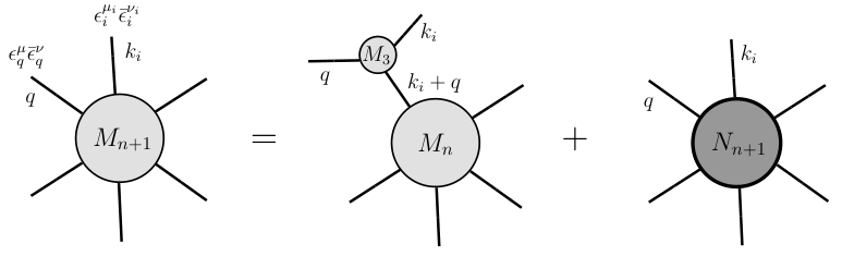
Figure 2: Decomposition of the -point massless closed string amplitude,
, into a factorizing part involving the three-point amplitude ,
where the soft state with momentum directly interacts with the th state,
exchanging a third massless closed state with momentum with
the -point amplitude , and the reminding part of the amplitude,
, which excludes factorization through the former channel.
By using the expression for the three-point amplitude in
Eq. (4.49), specialized to gravitons in the field theory
limit , it has been shown in Ref. [10] that by
decomposing the point amplitude as in Fig. 2,
and imposing gauge invariance, i.e. , one exactly recovers the tree-level
soft graviton theorem to subsubleading order. In the previous sections
we have explicitly shown to subsubleading order and for a finite value
of (see also Ref. [14]) that the same
gauge invariance also applies to amplitudes where the external states
can, as well as gravitons, be dilatons and Kalb-Ramond states.
Based on this, it was shown in Ref. [3] that
in the limit the dilaton soft theorem to subsubleading
order can be found also using just gauge invariance of the on-shell amplitude.
(In Ref. [3] only the cases where the other hard states
are either dilatons or gravitons were considered, however, the extension to
also include the antisymmetric Kalb-Ramond states trivially yields the
expression found in Eq. (3.43).) Now we extend this
line of analysis to also involve the string corrections to the three-point
amplitude.
We first decompose the -point amplitude as
in Fig. 2, reading:
(4.56)
where dependence on all other is implicit. The indices
belong to the soft state with momentum , and we
assume them to be symmetric, i.e. .
We now use the explicit form of the three-point string amplitude, , and
focus here only on the -terms.
We can read off these terms, when is symmetric, from
Eq. (4.55), and as we noticed before, they can be
rewritten as an operator by using Eq. (3.39), when
they are multiplied . Thus we have:
(4.57)
Now, imposing on-shell gauge invariance of the amplitude, we first find from , and Taylor expanding in :
(4.58a)
(4.58b)
Inserting this back into the Taylor-expanded form of Eq. (4.57), and imposing also , we get:
(4.59)
Thus, in total we find:
(4.60)
which demonstrates that, when the soft state is a graviton or a dilaton, on-shell gauge invariance of the string amplitude implies a soft theorem at subsubleading order even when string corrections are taken into account.
Finally we can rewrite this expression as:
(4.61)
This is exactly the expression we found in Eq. (2.34)
from explicit calculations. As we noticed in Eq. (3.43),
this expression vanishes when contracted with the polarization of the dilaton.
For the graviton, we have explained that the term singular in comes
from the exchange diagram where the the soft graviton scatters on an external
massless closed string. When that string is a graviton, respectively, dilaton, the
exchanged states is the opposite, i.e. a dilaton, respectively, graviton, meaning
that the -point amplitude in the soft theorem may involve other external
hard states, than those specified in the -point amplitude.
The non-singular terms on the other hand are, as we have shown, direct
consequences of on-shell gauge invariance.
For the sake of completeness we conclude this section by comparing to the low-energy
effective action that appears in Ref. [20], given by
(4.62)
where, with respect to Eq. (3.1) of Ref. [20], we have chosen a
different overall
normalization and have introduced a canonically normalized dilaton. The
first line corresponds to the field theory limit and from it we can reproduce
the two first couplings in Eq. (4.50) together with the field theoretical
three-graviton amplitude.
The second line shows the string corrections linear in , where we have only written down the terms that gives corrections to the three-point amplitude, while the ellipsis denotes the higher-point operators.
In particular, the last coupling in Eq. (4.50) is reproduced
by taking the lowest term of the Gauss-Bonnet part together with a dilaton coming from
the exponential in front of the Gauss-Bonnet term, while the cubic term
in the metric coming from only the Gauss-Bonnet part reproduces the first
string correction to the three-graviton amplitude in Eq. (4.49),
as already noticed in Ref. [22].
Discussion and Conclusion
In this paper we completed the computation of the amplitude involving massless closed string states in the bosonic string to the subsubleading order in the soft momentum expansion of one of the external states. When the soft state is either a graviton or a dilaton we showed that the result can be expressed as a soft theorem to subsubleading order. The graviton soft theorem has string corrections at the subsubleading order in the bosonic string, while the string corrections for the dilaton all vanish. The leading and subleading terms
were already obtained in Ref. [14].
The calculation involves an extension of the technique developed in
Ref. [14], which is rather involved, but the final result has a very simple explanation:
The basic ingredients to derive the soft-theorems are gauge invariance and the three-point amplitude with massless closed string states that, in the bosonic string, contains also string corrections. The procedure is an extension of the one followed in
Ref. [10], where the total amplitude is written as a sum of two types of terms.
One corresponds to diagrams where the soft leg is attached to each of the
other external legs through the three-point amplitude of the soft state
and two other massless states. These terms trivially factorize and in general have a pole when the momentum of the soft state goes to zero. The other type of terms do not factorize trivially and are finite in the soft limit. The two types of contributions, however, are not separately gauge invariant.
Thus, by imposing on-shell gauge invariance of the full amplitude, one is able to
factorize the soft behavior of the total amplitude up to subsubleading order in
the soft momentum. With respect to the procedure of Ref. [10] for the
case of a soft graviton, there are, however, two important differences.
Gauge invariance
imposed on the amplitude does not only give the soft behavior
for the graviton, when saturated with the graviton polarization
, but also that for the dilaton when saturated with the
polarization of the dilaton . The second difference with
respect to the field theoretical behavior of an amplitude with only gravitons,
is that, in general, the state exchanged in the propagator of the pole term
is not necessarily the same that appears in the corresponding external leg.
This happens in the string correction term in the amplitude with only gravitons
and in the case of a soft dilaton.
We thus arrive to the conclusion that the soft theorems for
the graviton and the dilaton are both consequence of gauge invariance and
that the string corrections appearing at subsubleading order for the graviton are direct consequences of the three-point amplitude with massless closed strings
having string corrections in the bosonic string. Since the three-point amplitude in superstring
has no string corrections, we expect no string corrections in the soft behavior
of a graviton in superstring.
A curious outcome of our results is that the soft theorem of a dilaton contains, at subleading
order, the generator of scale transformation and, at subsubleading order, the
generator of special conformal transformations as is also the case in the
soft theorem of a Nambu-Goldstone boson of spontaneously broken
conformal symmetry [3]. Some discussions of this was given in Ref. [3], but it would be interesting to have a more physical
understanding of why this happens. Finally, it would also be interesting to
extend our considerations to the soft behavior of the Kalb-Ramond
antisymmetric tensor, and furthermore how the results go over to the case of superstrings.
Acknowledgments
We thank Massimo Bianchi, Marco Billò, Marialuisa Frau, Andrea Guerrieri,
Alberto Lerda, Carlo Maccaferri, Josh Nohle, Igor Pesando and Congkao Wen for many useful discussions. We owe special thanks to Josh Nohle for many relevant comments
on our results.
Appendix A Results of integrals
All integrals necessary for the results of this paper can be reduced to the general form:
(A.63)
We are using the convention . The quantity is symmetric in its lower, respectively upper indices and complex conjugation exchanges the lower and upper indices.
These integrals can generically be evaluated after an expansion in by a substitution of the form .
It can be useful to substitute further , such that , enabling use of Cauchy’s integral formula over the unit circle.
To evaluate the integrals one must consider, case by case, when indices of are equal or not. Thus, in the following different labels on indices indicates the case when they are not equal to each other.
We have explicitly computed all integrals to the relevant order in involved in this paper using the mentioned procedure. Through this procedure, in Ref. [14] the integrals and were already computed to the order , with the results:
(A.64)
(A.65)
where is a cutoff that vanishes, when inserted in the appropriate expression.
It is useful to express the symmetrized and antisymmetrized form of latter expressions:
(A.66)
(A.67)
It is a long and tedious exercise to evaluate all other integrals by the above mentioned procedure.
In this appendix we therefore instead present an alternative shorter derivation leading to the same results, by making use of the above two expressions.
By using partial derivatives with respect to the ’s it is possible to directly get the higher-index integrals from the two basic integrals above. The following four integrals for instance are readily derived in this way, and they will be used, together with the previous two integrals, as master integrals as will be explained below:
(A.68)
(A.69)
(A.70)
(A.71)
All the other integrals relevant in the soft limit are related to the six master integrals by simple algebraic relations which follows from a useful rewriting of the holomorphic and anti-holomorphic poles of Eq. (A.63). has poles both in , and in , . It can be written as linear combination of the quantities , , having only two of the above mentioned poles. This follows from the identity:
(A.72)
with a similar relation for the variable. This determines:
(A.73)
By applying Eq. (A.73) iteratively, all the necessary integrals can be computed.
Following such an analysis, we present in the subsequent sections the results of all integrals involved in this work to the necessary order in .
It will be useful to notice from the above decomposition that an integral can yield a term of order only if one of its lower indices is equal to one of the upper ones, since its decomposition may only then contain . This property will be used throughout our derivations.
Integrals of the form
The integrals and were already given above in Eqs. (A.70)-(A.71).
The quantities and have been computed up to the order and therefore we could give up to this order in the soft expansion. However, this integral appears in and multiplied by a factor , therefore, only the terms of order are relevant.
This kind of restriction will be implicit in all the following results.
Then,
(A.75)
(A.76)
(A.77)
(A.78)
As we have already noticed, the expansion of the integrals may start from order only if one of the upper indices is equal to one of the lower ones. Thus the result of Eq. (A.78) could have been readily inferred from this property, without making the intermediate decomposition. This example serves as a demonstration of this property, which we will directly use for the rest of this appendix.
The result of the last integral follows immediately due to non of the upper and lower indices being pairwise equal.
Integrals of the form
Using Eq. (A.73) iteratively, and the identities and , where denotes the complex conjugate, we get
(A.84)
(A.85)
(A.86)
(A.87)
(A.88)
(A.89)
Finally, the integrals , , have either all the upper indices different from the lower ones or more than one lower index equal to an upper one. Thus according to the general property, noticed specifically after Eq. (A.78), we have:
The last result follows since none of the lower indices are equal to the upper ones.
Integrals of the form
For these integrals either two upper indices are equal to some lower indices, or
none are equal. Thus neither of the cases contains in its decomposition and thus in any case,
(A.100)
Appendix B Matching with the subsubleading soft operator
In this appendix we explicitly show how our main result in
Eq. (2.34) reproduces our explicit calculation
of the amplitude of massless closed states in the bosonic
string, presented in Sect. 2 and App. A, when
the soft state is a graviton or a dilaton.
In Eq. (2.34), the subsubleading soft operator is the sum of
four parts which act on the -point amplitude. The result of this action is
given
below and compared with explicit results in Eqs. (2.20)-(2.22).
The action of the first term in Eq. (2.34) on the -point
amplitude is:
(B.101)
We are denoting with , , terms with different powers in the Grassmann variables .
The action of the second operator in Eq. (2.34) gives:
(B.102)
The action of the operators in the second and third line of Eq. (2.34) will be considered in the end.
We restrict our analysis to the case in which the external soft particle
is a graviton or a dilaton, meaning that the expressions above are projected on the symmetric combination of .
All depend on the polarizations and momenta of the hard particles. Their explicit expressions are rather lengthy, but we may express them in more compact terms by using the explicit expressions for the quantities given in App. A, which also allows for an easier identification with the expression in Eqs. (2.20)-(2.22). The first quantity can be expressed as:
(B.103)
with .
This expression is real and thus the terms simply give a factor of two.
Because of this factor , the term with in
Eq. (B.103) cancel the analogous term in
Eq. (B.102).
The remaining term in Eq. (B.103) involving coincides with
the symmetric part of in Eq. (2.20a).
The next term reads:
(B.104)
The first three terms and their complex conjugate cancel the first three
terms in Eq. (B.102) and their complex conjugate,
coming from the second soft operator.
The third line of this expression makes up part of when the soft state is taken to be symmetrically polarized, i.e .
The following terms of then remain to be matched:
(B.105)
The last term in Eq. (B.104) is equal to when the soft state again is a graviton or a dilaton.
Finally, the second line does not match any term in , and , but they will be cancelled by the additional soft operators, discussed in the end, which at the same time will also produce the missing terms in Eq. (B.105).
Next, we consider
(B.106)
For the terms involving we can show that they are matched by part of the first term in , by using the following identities:
(B.107)
The first term of furthermore contains the following term, unmatched by Eq. (B.106):
(B.108)
The terms involving in Eq. (B.106) trivially reproduce the first part of . Finally, the first and the last line in Eq. (B.106) are not present in , and .
Again, we discuss on the missing pieces in the end.
Next, we consider
(B.109)
The first line, the first term of the second line, and the last term are all real, so their complex conjugate simply brings a factor of two. We may use the following identities to show that the first and second line and the first term in the third line match the second part of :
(B.110)
The last term in Eq. (B.109) is trivially matched by and all the remaining terms are matched by the second part of .
Next, consider
(B.111)
It is easily seen that this expression matches the first part of through order , after using the identities
(B.112)
and the property that only contributes at order if either of the indices or equals .
Next, we consider
(B.113)
The terms in the first line match , since and .
For the remaining terms, all the dependence on the variables in the second line is matched by the integrals , while dependence on the variables in the third line, instead, matches the integrals . Finally the last two terms follow respectively from the integrals and . Altogether these remaining terms thus match the second part of .
The last expression to be considered is
(B.114)
The first line can be expressed in terms of the integrals , matching the similar type of terms in . Similarly the other terms can be expressed in terms of the integrals , , and , matching the remaining types of non-vanishing terms in .
Finally, by the same procedures as above, it is easy to check that the remaining terms to be matched in Eqs. (B.105) and (B.108) are obtained by acting on the -point amplitude with the operators defined in the second and third line of Eq. (2.34). These operator simultaneously produce terms, which exactly cancel the unmatched terms in Eqs. (B.104) and (B.106). This proves the uniqueness of the subsubleading soft operator in Eq. (2.34) applicable to the graviton and the dilaton.