Interacting Quintessence in a New Scalar-Torsion Gravity

A mysterious component of our universe is dark energy. It is responsible for current cosmic acceleration and observationally confirmed [1-4]. $\Lambda$CDM model is the simplest theoretical explanation for dark energy in which a cosmological constant $\Lambda$ accounts for dark energy and it is in best agreement with the observational data. Besides its successes, $\Lambda$ suffers from two major problems: the so-called cosmological constant problem and the cosmic coincidence problem [5, 6].
To solve these problems, one needs to introduce further dynamical degrees of freedom, either by modifying the right hand side of the Einstein equations or the left hand side of them. In the first class usually a scalar field such as quintessence [7], phantom [8], tachyon [9] and so on, appears in the source sector while in the second class the Ricci scalar $R$ is replaced by often higher order terms in the gravitational field. The well-known $f(R)$ [10, 11], $f(G)$ [12, 13] and $f(R,G)$ [14-16] models belong to this later class and it is proved that after some transformations and redefinitions these theories can be recast into scalar-tensor theories.
In scalar-tensor theories such as the Brans-Dick theory [17], scalar field non-minimally couples to gravity. The non-minimal coupling of the form $f(\varphi)R$ is motivated by many reasons such as quantum corrections, renormalizability of the scalar field theory in curved space, Klauze-Klein compactification scheme, the low-energy limit of superstring theory etc. The most general non-minimally coupled scalar field theory results in second order field equations, is known as the Horndeski model [18] in which higher order derivatives of the scalar field appear in its Lagrangian.
Furthermore, while dark energy models usually assume the filed to be non-interacting considering an interaction between different components of the universe could provide solutions to a number of cosmological problems such as the coincidence problem via the method of scaling solution [19-22]. In fact, as nothing specific is known about the nature of both dark energy and dark matter, there is no physical reason to exclude the possible interaction between them. In addition, there are some observational evidences for interaction in dark sectors of our universe [23, 24]. These facts motivate us to study a new proposed dark energy model in an interacting scenario.
Moreover, an alternative gravitational theory to general relativity is the teleparallel gravity where gravity is described by using the Weitzenbock connection (for review see [25]). The Lagrangian of this theory is written with the torsion scalar $T$, and not the Ricci scalar $R$ defined with Levi-Civita connection [26-28] as in general relativity.
Recently inspired by the same theories in the framework of general relativity, various generalization of teleparallel gravity including $f(T)$ gravity [29-31], $f(T,T_{G})$ gravity [32] as well as non-minimally coupled scalar-torsion theories [33] have been wildly studied in the literature (see for example [34, 35]).
A non-minimal coupling between derivative of scalar field and curvature in the framework of general relativity is also another interesting issue to explore cosmological implications of such a coupling in details [36-38]. The same non-minimal coupling of the form $T\,g^{\mu\nu}\,\partial_{\mu}\varphi\partial_{\nu}\varphi$ is considered in [39] to obtain black hole solution of the model in teleparallel framework.
A new version of the above mentioned scalar-torsion theory has been proposed in [40, 41] where scalar field through its derivatives couples to vector part of torsion in the form $f(\varphi)\,\partial_{\mu}\varphi\,\mathcal{V}^{\mu}$ with $\mathcal{V}^{\mu}$ as the vector torsion. Recently, Jennen and Pereira have shown in [54] that such a non-minimal coupling of scalar field derivative and vector torsion naturally appears in the context of de Sitter teleparallel gravity which is consistent with local space time kinematics regulated by the de Sitter group SO(1,4). In the present work we study the dynamics of such a model by considering an interaction between dark energy and background matter. We perform a detailed phase-space analysis of the model for the most familiar interaction term extensively considered in the literature. The present paper is organized as follows:
In section 2 we briefly review the teleparallel gravity and then introduce the model. In section 3 by using suitable auxiliary variables we build up a system of autonomous differential equations. In section 4, the critical points of dynamical system are extracted for constant $\alpha$ (it means the coupling function is linear in terms of $\varphi$). Fixed points and their stability properties for a non-constant $\alpha$ have been obtained in section 5. Section 6 is devoted to our conclusion.

Here we briefly review the formulation of teleparallelism. The metric is written as $g_{\mu\nu}=\eta_{ab}\,e_{\mu}^{a}\,e_{\nu}^{b}$ where $\eta_{ab}$ is the Minkowski metric, $e_{a}(x^{\mu})$ are orthonormal tetrad components at points $x^{\mu}$ of the manifold in the tangent space and $e_{a}^{\mu}$ is the tangent vector of the manifold. As we mentioned earlier the Lagrangian density is given by torsion scalar $T$ defined as $T\equiv S_{\rho}\,^{\mu\nu}T^{\rho}\,_{\mu\nu}$, where $T^{\rho}\,_{\mu\nu}\equiv e_{a}^{\rho}\big(\partial_{\mu}e^{a}_{\nu}-\partial_{\nu}e^{a}_{\mu}\big)$ is the torsion tensor and $S_{\rho}\,^{\mu\nu}\equiv\frac{1}{2}\big(K^{\mu\nu}\,_{\rho}+\delta^{\mu}_{\rho}\,T^{\alpha\nu}\,_{\alpha}-\delta^{\nu}_{\rho}\,T^{\alpha\mu}\,_{\alpha}\big)$ with $K^{\mu\nu}\,_{\rho}\equiv-\frac{1}{2}\big(T^{\mu\nu}\,_{\rho}-T^{\nu\mu}\,_{\rho}-T_{\rho}\,^{\mu\nu}\big)$ is the contorsion tensor.
By considering the FRW metric background as

$\displaystyle ds^{2}=dt^{2}-a^{2}(t)(dr^{2}+r^{2}d\Omega^{2}),$

(1)

the metric and tetrad components read $g_{\mu\nu}=diag(1,-a^{2},-a^{2},-a^{2})$ and $e^{a}_{\mu}=(1,a,a,a)$ respectively. In FRW background the torsion scalar is also given by $T=-6H^{2}$. Here, $H=\frac{\dot{a}}{a}$ is the Hubble parameter, $a$ is the scale factor and a dot stands for derivative with respect to the cosmic time $t$.
Furthermore, the torsion scalar can be decomposed into three components namely vector torsion, axial torsion and pure tensor torsion [25] where by vector torsion we mean

$$\mathcal{V}_{\mu}=T_{\,\,\nu\mu}^{\nu}.$$

(2)

The Ricci scalar of the Levi-Civita connection in terms of the Weitzenbock connection can be expressed as

$$R=-T+2\nabla_{\mu}\,\mathcal{V}^{\mu}=-T+\frac{2}{e}\partial_{\mu}\,(e\mathcal{V}^{\mu}),$$

(3)

where $\nabla_{\mu}$ is the Levi-Civita covariant derivative.
Moreover, a non-minimal coupling between a scalar field and the Ricci scalar of the form $\xi R\varphi^{2}$, because of the motivations such as quantum corrections to the scalar field in curved space-time [46-47], renormalization considerations [48] and its appearance in the context of superstring theories [49] is completely reasonable.
Now, if ones try to construct the same theory in the teleparallel framework, they should consider a non-minimal coupling between scalar field and the boundary term (total derivative term in (3) [50, 51]) of the form $C(\varphi)\nabla_{\mu}\,\mathcal{V}^{\mu}$. However, integration by parts from such a coupling leads to the following equivalent coupling $f(\varphi)\,\mathcal{V}^{\mu}\partial_{\mu}\varphi$ where $f(\varphi)=C^{\prime}(\varphi)$ and this is the form of coupling we will consider in the following.
Now let us introduce the model in which scalar field non-minimally couples to the vector torsion through its derivative

$$S=\int d^{4}x\,e\,\left[\frac{T}{2\,\kappa^{2}}-\frac{1}{2}\partial_{\mu}\varphi\partial^{\mu}\varphi-V(\varphi)+\eta\,f(\varphi)\partial_{\mu}\varphi\,\mathcal{V}^{\mu}\right]+S_{m},$$

(4)

where $e\equiv\det(e^{a}_{~\mu})=\sqrt{-g}$, $\kappa^{2}=8\pi G$ and $G$ is a bare gravitational constant (for reviews on teleparallelism see [25]). $S_{m}$ is the matter action, $\eta$ is a dimensionless constant measuring the non-minimal coupling and $f(\varphi)$ is an general function of the scalar field.
The gravitational coupling of fundamental fields in teleparallel gravity is a controversial subject. Since there is no experimental data to help us, we should rely on equivalence between general relativity and teleparallel gravity. According to this formulation, each one of the fundamental fields of nature (scalar, spinor, and electromagnetic) are required to couple to torsion in such a way to preserve the equivalence between teleparallel gravity and general relativity. It is shown in [25] that in the context of teleparallel gravity a scalar field by itself does not feel gravity but its four-derivative (which is a vector field) interacts with the vector part of the torsion. On the other hand, in the framework of teleparallelism, due to the presence of a total derivative in the relation between the curvature scalar and the torsion scalar the essential condition for the torsion scalar $T$ to has its non-minimal coupling to a scalar field in a conformal manner is that a term of the form $f(\varphi)\partial_{\mu}\varphi\,\mathcal{V}^{\mu}$ has to be assumed in the action [52]. Also, it has been shown in Ref [53] that a Lagrangian which is invariant under the space-time coordinate transformations and conformal transformations and leads to teleparallel Lagrangian in the gauge where the scalar field is restricted to assume a constant value, includes a non-minimal coupling of the form $g^{\mu\nu}\,\mathcal{V}_{\nu}\varphi\,(\partial_{\mu}\varphi)$.
The model (4) and teleparallel dark energy model [33] in which scalar field non-minimally coupled to the torsion scalar instead of vector torsion, are mathematically related through a conformal transformation although they are physically different. In what follows we consider a possible interaction between dark energy and dark matter and study the phase-space of the model (4).
Varying action (4) with respect to the tetrad field yields to the field equations. In this procedure the energy momentum tensor associated with the scalar field $\Theta_{a}\vskip 0.28453pt^{\rho}\equiv-\frac{1}{e}\frac{\delta S_{\varphi}}{\delta e^{a}\vskip 0.28453pt_{\rho}}$ is given by

$$\Theta_{a}\vskip 0.28453pt^{\rho}=\eta\big[f(\varphi)(\mathcal{V}^{\rho}\partial_{a}\varphi+\nabla_{a}\partial^{\rho}\varphi-e_{a}\vskip 0.28453pt^{\rho}\nabla_{\mu}\partial^{\mu}\varphi)+f_{,\varphi}(\partial_{a}\varphi\,\partial^{\rho}\varphi-e_{a}\vskip 0.28453pt^{\rho}\partial_{\mu}\varphi\,\partial^{\mu}\varphi)\big]$$

$$-e_{a}\vskip 0.28453pt^{\rho}\big(\frac{1}{2}\partial_{\mu}\varphi\,\partial^{\mu}\varphi-V(\varphi)\big)+\partial_{a}\varphi\,\partial^{\rho}\varphi,$$

(5)

where $\nabla^{\mu}$ is the covariant derivative in the teleparallel connection [25], $f_{,\varphi}=\frac{df(\varphi)}{d\varphi}$ and $V_{,\varphi}=\frac{dV}{d\varphi}$.
By imposing the flat FRW metric in (5), we obtain the Friedmann equations with scalar field energy density and pressure of the form,

$$\rho_{\varphi}=\frac{1}{2}\dot{\varphi}^{2}+V(\varphi)-3\eta f(\varphi)H\dot{\varphi},$$

(6)

and

$$p_{\varphi}=\frac{1}{2}(1+2\,\eta\,f_{,\varphi})\dot{\varphi}^{2}-V(\varphi)+\eta f(\varphi)\ddot{\varphi}.$$

(7)

Additionally, variation of action (4) with respect to the scalar field yields to its evolution equation that in FRW background takes the form

$$\ddot{\varphi}+3\,H\,\dot{\varphi}-3\,\eta\,\left(\dot{H}+3H^{2}\right)\,f(\varphi)+V_{,\varphi}=-\frac{Q}{\dot{\varphi}},$$

(8)

where $Q$ is a general interaction term corresponding to coupling between dark energy and dark matter. In fact equation (8) expresses the continuity relation for the field $\dot{\rho}_{\varphi}+3\,H\left(1+\omega_{\varphi}\right)\rho_{\varphi}=-Q$ with $\omega_{\varphi}=p_{\varphi}/\rho_{\varphi}$ the equation of state of the scalar field while the continuity equation for matter reads $\dot{\rho}_{m}+3H(1+\omega_{m})\rho_{m}=Q$.
Here, we mention that considering an interaction between dark energy and dark matter is a common way for elaboration of the well-known coincidence problem or why are the densities of vacuum energy and dark matter equal today? In dynamical system technique this problem can be alleviated via the method of scaling solutions [19-22] (solution corresponding to accelerating universe and ratio $\frac{\rho_{\varphi}}{\rho_{m}}=c$, with $c$ a non-zero constant).

In order to study the phase-space and stability analysis of the model using the dynamical system method let us introduce the following auxiliary variables:

$$x\equiv\frac{\kappa\,\dot{\varphi}}{\sqrt{6}\,H},\>\>\>\>\>\>y\equiv\frac{\kappa\,\sqrt{V}}{\sqrt{3}\,H},\>\>\>\>\>\>u\equiv\kappa\,f,\>\>\>\>\ \alpha\equiv f_{,\varphi},\>\>\>\>\lambda\equiv-\frac{V_{,\varphi}}{\kappa V}.$$

(9)

In terms of these new variables, the field equations can be rewritten as follows,

$$\frac{dx}{dN}=(3-s)\Big(-x+\frac{\sqrt{6}}{2}\eta u\Big)+\frac{\sqrt{6}}{2}\,\lambda\,y^{2}-\hat{Q},$$

(10)

$$\frac{dy}{dN}=\left(-\frac{\sqrt{6}\,\lambda}{2}\,x\,y+s\right)\,y,$$

(11)

$$\frac{du}{dN}=\sqrt{6}\,\alpha\,x,$$

(12)

$$\frac{d\lambda}{dN}=-\sqrt{6}\,\lambda^{2}\,x\,\left(\Gamma-1\right),$$

(13)

$$\frac{d\alpha}{dN}=\sqrt{6}\,x\,\Pi,$$

(14)

where $N=\ln{a}$, $\hat{Q}=\frac{\kappa\,Q}{\sqrt{6}\,H^{2}\,\dot{\varphi}}$ and the following parameters are defined

$$\Pi=\frac{f_{,\varphi\varphi}}{\kappa},\>\>\>\>\>\>\>\>\>\>\>\Gamma=\frac{V\,V_{,\varphi\varphi}}{V_{,\varphi}^{2}}.$$

(15)

Also, $s$ in our setup reads,

$$s=-\frac{\dot{H}}{H^{2}}=3\,\left(\frac{2}{3}+\eta^{2}u^{2}\right)^{-1}\\ \left[2x^{2}(1+\eta\alpha)+2\sqrt{6}\eta xu+3\eta^{2}u^{2}+\lambda\eta y^{2}u+\gamma(1-x^{2}-y^{2}+\sqrt{6}\eta ux)-\sqrt{\frac{2}{3}}\eta u\hat{Q}\right],$$

(16)

where $\gamma$ is the barotropic index defined by $\gamma=1+\omega_{m}$ such that $1<\gamma<2$.
Using variables (9) the density parameters $\Omega_{i}\equiv(\kappa^{2}\,\rho_{i})/(3\,H^{2})$ for the scalar field and background matter are given by

$$\Omega_{\varphi}=x^{2}+{y}^{2}-\sqrt{6}\,\eta\,u\,x,\>\>\>\>\>\>\>\>\Omega_{m}=1-\Omega_{\varphi}.$$

(17)

Also the equation of state of the field $\omega_{\varphi}$, the effective equation of state and deceleration parameter $q$ can be written as

$$\omega_{\varphi}=\frac{p_{\varphi}}{\rho_{\varphi}}=\frac{(1+2\,\eta\,\alpha)x^{2}-y^{2}+\eta\,u\,\big(-\sqrt{6}x+\eta\,u(3-s)+\lambda\,y^{2}-\sqrt{\frac{2}{3}}\hat{Q}\big)}{x^{2}+{y}^{2}-\sqrt{6}\,\eta\,u\,x},$$

(18)

$$\omega_{eff}=\left(p_{\varphi}+p_{m}\right)/\left(\rho_{\varphi}+\rho_{m}\right)\\ =\left(\gamma-1\right)\big[1-(x^{2}+{y}^{2}-\sqrt{6}\,\eta\,u\,x)\big]+(1+2\,\eta\,\alpha)x^{2}-y^{2}+\eta\,u\,\big(-\sqrt{6}x+\eta\,u(3-s)+\lambda\,y^{2}-\sqrt{\frac{2}{3}}\hat{Q}\big).$$

(19)

and

$$q\equiv-1-\frac{\dot{H}}{H^{2}}=\frac{1}{2}+\frac{3}{2}\omega_{eff}.$$

(20)

In what follows we utilize $\omega_{eff}<-\frac{1}{3}$ to obtain the required conditions for an accelerating universe.
At this point we briefly review the dynamical system method and its autonomous system of equations. An autonomous system in general can be written as $\frac{d\textbf{Y}}{d\ln a}=f(\textbf{Y})$, where the column vector Y is constituted by suitable auxiliary variables and $f(\textbf{Y})$ is the corresponding column vector of the autonomous equations [42-44].
The solutions of the system of differential equations namely the solutions of $f(\textbf{Y})=0$, yield to the fixed (critical) points $\textbf{Y}_{c}$ of the system. In order to study the stability of the equilibrium or critical points we should first expand the system around $\textbf{Y}_{c}$ as $\textbf{Y}=\textbf{Y}_{c}+\textbf{U}$ where the column vector U denotes the perturbation of the variables. For each critical point the 1st order perturbation technique leads to the matrix equation $\textbf{U}^{\prime}=\Sigma.\textbf{U}$ where the matrix $\Sigma$ contains all the coefficients of the perturbation equations. The stability of the critical points can be obtained from the sign of the eigenvalues of $\Sigma$. If the real part of all eigenvalues at a fixed point are negative then the fixed point is a stable point otherwise it is an unstable one or a saddle (in fact if all the eigenvalues have positive real part, then the fixed point is an unstable fixed point and if some eigenvalues have negative real part and remaining eigenvalues have positive real part, then it is a saddle point). A detailed analysis of the stability criteria is given in Refs [42-44]. A critical point is an attractor when it is a stable point and the universe evolves to the attractor solutions regardless of the initial conditions.
In our setup once the parameters $\Gamma$ and $\Pi$ are known, equations (10)-(14) become a system of autonomous differential equations and one can study dynamics of the model in a usual way. Considering an exponential potential of the form $V=V_{0}\,e^{-\lambda\kappa\varphi}$ with constant $\lambda$ leads to $\Gamma=1$ and equation (13) can be eliminated from our system of differential equations. In the other hand, we classify our study in two parts. First, we consider a coupling function of the form $f(\varphi)\propto\varphi$ which yields to a constant $\alpha$. Consequently for an exponential potential and a constant $\alpha$ our system of autonomous equations is reduced to equations (10)-(12). In the second step a dynamically changing $\alpha$ is studied. For this case we mention that $u=\kappa\,f$ is a function of $\varphi$ and one can express $\varphi$ as a function of $u$ using the inverse function i.e $\varphi(u)=f^{-1}\big(\frac{u}{\kappa}\big)$. Thus, $\alpha(\varphi)$ and $\Pi(\varphi)$ can be written in terms of $u$ and the dynamical system described by equations (10)-(12) (for details see [45]).
In the following sections we extract the critical points and their properties for constant and dynamically changing $\alpha$. Also the interaction between dark energy and dark matter is assumed to be of the form $Q=\beta\,\kappa\,\rho_{m}\,\dot{\varphi}$ which leads to the following $\hat{Q}$ in equation (10)

$$\hat{Q}=\sqrt{\frac{3}{2}}\,\beta\,\Omega_{m},$$

(21)

where $\beta$ is a dimensionless constant.

In this section we assume that $\alpha$ in (9) is a no-zero constant. This means that the non-minimal coupling function is proportional to $\varphi$ i.e $f(\varphi)\propto\varphi$. By inserting (21) in (10), the dynamical system (10)-(12) has two critical points $A_{1}$ and $A_{2}$ presented in Table 1. This table also provides the corresponding values of density $(\Omega_{\varphi})$ and equation of state $(\omega_{\varphi})$ parameters of dark energy as well as the effective equation of state $(\omega_{eff})$ at each critical points.
Now substituting the liner perturbations $x\rightarrow x_{c}+\delta x$, $y\rightarrow y_{c}+\delta y$ and $u\rightarrow u_{c}+\delta u$ into the autonomous system (10)-(12) and linearize them give us the components of the perturbation matrix $\Sigma$ (the component of $\Sigma$ have been written in the Appendix). The sign of the real part of the eigenvalues of $\Sigma$ will determine the type and stability of the critical points. The results of stability analysis have been summarized in Table 2. We have also presented the existence and acceleration conditions in Table 2. Let us now discuss the properties of critical points in details.

Critical Point $A_{1}$:
This point corresponds to a completely dark energy dominated solution $(\Omega_{\varphi}=1)$ with equation of state equal to the cosmological constant $(\omega_{\varphi}=1)$. Accelerated expansion occurs at point $A_{1}$ for all values of the model parameters. Three eigen values of matrix $\Sigma$ at this point are as follows:

$$\mu_{12}=\frac{3}{2}\Big(-1\pm\sqrt{1+\frac{24\,\eta\,\alpha}{\lambda^{2}+6}}\Big),\,\,\,\,\,\,\,\,\mu_{3}=-3\gamma.$$

Therefore, $A_{1}$ is a stable point if $\eta\alpha<0$ and thus it can attract the universe at late-times.
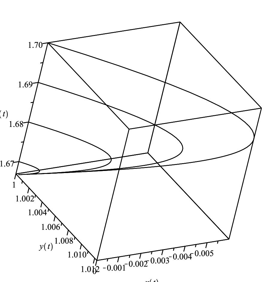
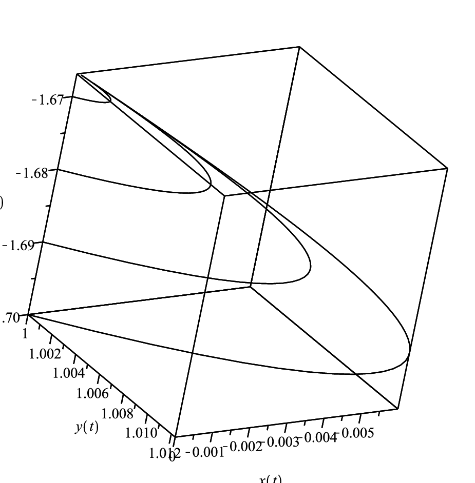
Using numerical computations and phase-space trajectories, we have shown the attractor behavior of point $A_{1}$ for special choices of the model parameters in Figure 1.

Critical Point $A_{2}$:
Point $A_{2}$ corresponds to a matter dominated solution that exists under condition $2\beta^{2}>12(\gamma-1)-3\gamma^{2}+2(\gamma-2)\gamma\,\eta$. The deceleration parameter at this point is given by $q=\frac{3}{2}\gamma-1$. Thus expansion of the universe is non-accelerating. Eigenvalues of linearized perturbation matrix at this point are obtained as,

$$\mu_{1,2}=\frac{3}{2}(\gamma-2)\Big(-1\pm\sqrt{1+\frac{2\,\gamma\,\eta\,(2-\gamma)}{(3\gamma^{2}+2\beta^{2}-12\gamma+12)}}\Big),\,\,\,\,\,\,\,\,\mu_{3}=\frac{3}{2}\gamma.$$

So, $A_{2}$ is an unstable point because one of the eigenvalues $(\mu_{3})$ is positive. It may deserve to be considered as a possible state of the universe at previous stages.

When the non-minimal coupling function is any general function of $\varphi$ other than $f(\varphi)\propto\varphi$ then the parameter $\alpha$ will be a non-constant parameter. As we mentioned in section 3, $\alpha$ can be expressed in terms of $u$ such that at critical point $(x_{c},y_{c},u_{c})$, $\alpha(u)\rightarrow\alpha(u_{c})=0$. Also when $(x,y,u)\rightarrow(x_{c},y_{c},u_{c})$, the field $\varphi$ rolls down toward $\pm\infty$ with $f(\varphi)\propto\frac{1}{\kappa}$ and $u_{c}=1$. Five critical points of dynamical system (10)-(12) together with the corresponding values of $\Omega_{\varphi}$, $\omega_{\varphi}$ and $\omega_{eff}$ are presented in Table 3. The existence conditions, acceleration and stability criteria of these points have been shown in Table 4. Detailed explanation for each point is as follows:

Critical Point $B_{1}$:
Point $B_{1}$ exists for all values of the model parameters. Dark energy density parameter $\Omega_{\varphi}$, equation of state $\omega_{\varphi}$, effective equation of state $\omega_{eff}$ and deceleration parameter $q$ at this point are given respectively by

$$\Omega_{\varphi}=-\frac{1}{6}\frac{(3\gamma\,\eta+2\beta-6\eta)(-6\beta\,\eta^{2}+3\gamma\,\eta-2\beta-6\eta)}{(-\beta\,\eta+\gamma-2)^{2}},$$

(22)

$$\omega_{\varphi}=\frac{-6\beta(\gamma-1)\eta^{2}+(3\gamma^{2}-2\beta^{2}-9\gamma+6)\eta-2\beta}{(-6\beta\,\eta^{2}+(3\gamma-6)\eta-2\beta)},$$

(23)

$$\omega_{eff}=\frac{1}{9}\,\frac{-2\beta^{2}+3(-2\gamma+3)\eta\,\beta+3\gamma(\gamma-3)+6}{(-\beta\,\eta+\gamma-2)},$$

(24)

and

$$q=\frac{1}{2}\,\frac{-2\beta^{2}+2(-3\gamma+4)\eta\,\beta+\gamma(3\gamma-8)+4}{(-\beta\,\eta+\gamma-2)}.$$

(25)

It is not easy to obtain a simple expression for acceleration condition $\omega_{eff}<-\frac{1}{3}$ using equation (24). Thus, we find the acceleration condition only when the matter is non-relativistic $(\gamma=1)$. In this case under the following conditions the expansion of the universe is accelerating

i)   if $(\beta\,\eta+1)>0$ then we need the parameter $\beta$ to be satisfied in

$$\frac{\eta}{2}\Big[1-\sqrt{1-\frac{2}{\eta^{2}}}\Big]<\beta<\frac{\eta}{2}\Big[1+\sqrt{1-\frac{2}{\eta^{2}}}\Big],$$

(26)

and

ii)   if $(\beta\,\eta+1)<0$ then we require

$$\beta>\frac{\eta}{2}\Big[1+\sqrt{1-\frac{2}{\eta^{2}}}\Big],$$

or

$$\beta<\frac{\eta}{2}\Big[1-\sqrt{1-\frac{2}{\eta^{2}}}\Big].$$

(27)

The solution $B_{1}$ can be a scaling solution $(0<\Omega_{\varphi}<1)$ for particular choices of the model parameters and hence give hope to alleviate the cosmological coincidence problem.
Three eigenvalues of the corresponding perturbation matrix $\Sigma$ at point $B_{1}$ read

$$\mu_{1}=\frac{-2\beta^{2}-6(\gamma-2)\eta\,\beta+3(\gamma-2)^{2}}{2(-\beta\,\eta+\gamma-2)},$$

$$\mu_{2}=\frac{\tau_{c}(3\gamma\,\eta+2\beta-6\eta)}{(-\beta\,\eta+\gamma-2)},$$

$$\mu_{3}=\frac{-2\beta^{2}-2\big(3(\gamma-1)\eta+\lambda\big)\beta+3(\gamma-2)(-\eta\,\lambda+\gamma)}{2(-\beta\,\eta+\gamma-2)},$$

(28)

where $\tau_{c}$ in $\mu_{2}$ stands for $\tau_{c}=\frac{d\alpha(u)}{du}|_{u=u_{c}}$. So, $B_{1}$ could be an attractor solution for different values of the model parameters.
Let us consider the simple case $\gamma=1$ and examine the stability conditions. In this case $B_{1}$ is a stable point under the following requirements:

i)   if $(\beta\,\eta+1)>0$ then one of the required conditions is as follows

$$-\frac{\lambda}{2}\Big[1+\sqrt{1+\frac{6(\eta\,\lambda-1)}{\lambda^{2}}}\Big]<\beta<\frac{\lambda}{2}\Big[-1+\sqrt{1+\frac{6(\eta\,\lambda-1)}{\lambda^{2}}}\Big],$$

(29)

and for $\tau_{c}<0$ the additional condition read

$$\frac{3}{2}\eta\Big[1-\sqrt{1+\frac{2}{3\eta^{2}}}\Big]<\beta<\frac{3}{2}\eta,$$

(30)

while for $\tau_{c}>0$ in addition to (29) one needs

$$\frac{3}{2}\eta<\beta<\frac{3}{2}\eta\Big[1+\sqrt{1+\frac{2}{3\eta^{2}}}\Big].$$

(31)

ii)   if $(\beta\,\eta+1)<0$ then for $B_{1}$ to be an stable point one requires

$$\beta>\frac{\lambda}{2}\Big[-1+\sqrt{1+\frac{6(\eta\,\lambda-1)}{\lambda^{2}}}\Big],$$

or

$$\beta<-\frac{\lambda}{2}\Big[1+\sqrt{1+\frac{6(\eta\,\lambda-1)}{\lambda^{2}}}\Big].$$

(32)

Additionally for $\tau_{c}<0$ we should have

$$\beta>\frac{3}{2}\eta\Big[1+\sqrt{1+\frac{2}{3\eta^{2}}}\Big],$$

(33)

and for $\tau_{c}>0$

$$\beta<\frac{3}{2}\eta\Big[1-\sqrt{1+\frac{2}{3\eta^{2}}}\Big].$$

(34)

All in all, point $B_{1}$ could be an attractor scaling solution in which accelerated expansion of the universe occurs. In the left panel Figure 2 we have depicted the phase-space trajectories of the model for special choices of parameters. With these values of parameters, $B_{1}$ is an attractor point as it is clear from the figure.

Critical Point $B_{2}$:
This point is a scalar field dominated solution $(\Omega_{\varphi}=1)$ but without accelerated expansion because $\omega_{eff}=1$. Since the eigenvalues of the corresponding matrix $\Sigma$ at point $B_{2}$ are very complicated, one can not conclude about its stability analytically. Thus, we should look at the phase-space trajectories to find whether this point is stable or not. Our numerical computations show that point $B_{2}$ is a stable point. Because of the disadvantage that the expansion is not accelerating, this point is not a realistic solution at late-times and we leave further explanations about point $B_{2}$.

Critical Point $B_{3}$:
Point $B_{3}$ has the same properties as point $B_{2}$. It exists for all values of model parameters, it is a stable dark energy dominated solution without accelerated expansion. Thus, we don’t pay attention to this point further.

Critical Point $B_{4}$:
The fixed point $B_{4}$ exists for

$$\beta>\frac{\lambda+3\eta(\gamma-1)}{2}\Big[-1+\sqrt{1-\frac{6(2-\gamma)(\gamma-\eta\,\lambda)}{\big(\lambda+3\eta(\gamma-1)\big)^{2}}}\Big],$$

or

$$\beta<-\frac{\lambda+3\eta(\gamma-1)}{2}\Big[1+\sqrt{1-\frac{6(2-\gamma)(\gamma-\eta\,\lambda)}{\big(\lambda+3\eta(\gamma-1)\big)^{2}}}\Big].$$

(35)

The expressions for $\Omega_{\varphi}$, $\omega_{\varphi}$, $\omega_{eff}$ and deceleration parameter $q$ at this point are given by

$$\Omega_{\varphi}=-\frac{1}{2}\frac{3\gamma\,\eta\,\lambda-2\beta^{2}+6\beta\,\eta-2\beta\,\lambda+6\eta\,\lambda-6\gamma}{(\beta+\lambda)^{2}},$$

(36)

$$\omega_{\varphi}=(\gamma-1)+\frac{2\gamma\,\beta\,(\beta+\lambda)}{3\eta\big(2\beta+(\gamma+2)\lambda\big)-2\beta\,(\beta+\lambda)-6\gamma},$$

(37)

$$\omega_{eff}=\frac{\gamma\,\lambda-\beta-\lambda}{\beta+\lambda},$$

(38)

and

$$q=\frac{3\gamma\,\lambda-2\beta-2\lambda}{2(\beta+\lambda)}.$$

(39)

Looking at equation (36), we conclude that point $B_{4}$ is a scaling solution $(0\leq\Omega_{\varphi}<1)$ for particular values of parameters $\eta$, $\lambda$, $\beta$ and $\gamma$. Thus this point can solve the coincidence problem.
Let us now examine the stability properties of this point. One of the eigenvalues of $3\times 3$ matrix $\Sigma$ at point $B_{4}$ is $\mu_{1}=\frac{3\tau_{c}\,\gamma}{\beta+\lambda}$, while two other eigenvalues are too complicated and hence we do not give their explicit expressions here. Numerically we find that if this point exists, it is stable and thus attract the universe at late-times. The conditions for stability of point $B_{4}$ is as follows

$$\tau_{c}>0\,\,\,\,and\,\,\,\,\beta+\lambda<0,$$

or

$$\tau_{c}<0\,\,\,\,and\,\,\,\,\beta+\lambda>0.$$

(40)

In the right panel of Figure 2 we have chosen the parameters such that they satisfy the above conditions. One can clearly see the attractor behavior of point $B_{4}$ in this figure. Another advantage of this point is that acceleration can be occurred under the following conditions

$$\beta<\frac{\lambda(3\gamma-2)}{2}\,\,\,\,and\,\,\,\,\beta+\lambda<0,$$

or

$$\beta>\frac{\lambda(3\gamma-2)}{2}\,\,\,\,and\,\,\,\,\beta+\lambda>0.$$

(41)

Critical Point $B_{5}$:
Similar to points $B_{2}$ and $B_{3}$, point $B_{5}$ is also a completely dark energy dominated solution $(\Omega_{\varphi}=1)$ that exists for

$$\eta\,\lambda<2,$$

and

$$-3\big(\eta+\sqrt{\frac{2}{3}+\eta^{2}}\big)<\lambda<3\big(-\eta+\sqrt{\frac{2}{3}+\eta^{2}}\big).$$

(42)

Dark energy equation of state, effective equation of state and deceleration parameter at point $B_{5}$ are as follows:

$$\omega_{\varphi}=\frac{1}{3}\,\frac{9\eta\,\lambda+2\lambda^{2}-6}{2-\eta\,\lambda},$$

(43)

$$\omega_{eff}=\frac{1}{3}\,\frac{9\eta\,\lambda+2\lambda^{2}-6}{2-\eta\,\lambda},$$

(44)

and

$$q=\frac{4\eta\,\lambda+\lambda^{2}-2}{2-\eta\,\lambda}.$$

(45)

Using equation (44) the required condition for acceleration $(\omega_{eff}<-\frac{1}{3})$ can be obtained as

$$-2\eta\Big[1+\sqrt{1+\frac{1}{2\eta^{2}}}\Big]<\lambda<2\eta\Big[-1+\sqrt{1+\frac{1}{2\eta^{2}}}\Big].$$

(46)

Three eigenvalues of Jacobian matrix $\Sigma$ at point $B_{5}$ read,

$$\mu_{1}=\frac{6\eta\,\lambda+\lambda^{2}-6}{2-\eta\,\lambda},$$

$$\mu_{2}=\frac{2\tau_{c}(3\eta+\lambda)}{2-\eta\,\lambda},$$

$$\mu_{3}=\frac{2(\lambda^{2}-3\gamma)+3(\gamma+2)\eta\,\lambda+2\beta_{1}(\lambda+3\eta)}{2-\eta\,\lambda}.$$

(47)

Thus, this point is an attractor (stable) point if

$$-\frac{1}{4}\big(3\eta(\gamma+2)+2\beta\big)\Big[1+\sqrt{1-\frac{48(\beta\,\eta-\gamma)}{\big(3\eta(\gamma+2)+2\beta\big)^{2}}}\Big]<\lambda<\frac{1}{4}\big(3\eta(\gamma+2)+2\beta\big)\Big[-1+\sqrt{1-\frac{48(\beta\,\eta-\gamma)}{\big(3\eta(\gamma+2)+2\beta\big)^{2}}}\Big].$$

(48)

Phase-space trajectories of the model for different initial conditions, have been plotted in Figure 3 such that the attractor behavior of point $B_{5}$ is transparent. Note however that, although point $B_{5}$ is an attractor solution of the autonomous system, it is not a scaling attractor and this is the disadvantage of point $B_{5}$.
The evolution of density parameters $\Omega_{\varphi}$ and $\Omega_{m}$ have been also depicted in Figure 4. In this figure we have considered $f(\varphi)=\frac{1}{\kappa}\big(1+e^{\kappa\varphi}\big)$ such that $\alpha(u)=-1+u$ and $\tau_{c}=1$. The present epoch $(N=4)$ corresponds to $\Omega_{\varphi}\approx 0.68$ and $\Omega_{m}\approx 0.32$.

Recently Otalora [40] has proposed a new teleparallel dark energy model in which the scalar field, responsible for dark energy, couples to vector torsion through its derivative. The model (4) is similar to the de Sitter teleparallel gravity, a theory consistent with local space-time kinematics regulated by the de Sitter group, proposed in Ref [54]. In such a theory gravitational sector modeled by teleparallel gravity interacts with the cosmological function due to a non-minimal coupling between the trace of the covariant derivative of the vierbein and a non-constant cosmological function $\Lambda$. Because the cosmological function is not restricted to be constant, its value can evolve during the cosmological evolution and thus may be suitable to describe the evolution of the universe from inflation to dark energy. As it is mentioned in [54] a huge cosmological term can drive inflation at the early universe and afterwards, it should decay to a small value to allow the structure formation of the universe. Then its value should somehow increase to account for the late-time accelerated expansion of the universe [60].
Additionally a conformally invariant extension of teleparallel gravity in which derivative of a scalar field non-minimally coupled to the vector torsion can realize a power-law or the de Sitter expansion of the universe and also can give rise to the $\Lambda$CDM model as it was shown in [52]. Later we studied the same model using a non-canonical scalar field (tachyon) instead of quintessence in the action [41]. Here we have generalized the Otalora^,s model by considering an interaction between dark sectors. Our basic goal was to examine whether there exist late-time scaling attractors, corresponding to a accelerated universe or not. Scaling attractors are those solutions that both density parameters of dark energy $(\Omega_{DE})$ and dark matter $(\Omega_{DM})$ are non-vanishing constants over there. Such a solutions can give hope to alleviate the cosmological coincidence problem and if they posses acceleration expansion, basic observational requirements will be satisfied.
Using dynamical system method we have extracted the critical points of the model for both constant and non-constant $\alpha$. When $\alpha$ is constant (it means the coupling function $f(\varphi)\propto\varphi$) we find two critical point $A_{1}$ and $A_{2}$ in Table 1. Neither $A_{1}$ nor $A_{2}$ are scaling attractors. For non-constant $\alpha$ there are five critical points presented in Table 3. In this case point $B_{1}$ and $B_{4}$ are scaling attractors under certain conditions for the free parameters of the model and they have the possibility to explain an accelerated universe. These two points make the main difference between interacting and non-interacting scenario at hand. While there is no scaling attractor in non-interacting scenario, one can switch on the interaction and obtain such solutions. The universe evolves to these attractor solutions for different initial conditions.
Before closing this section we mention some additional points: the post-Newtonian limit of teleparallel gravity with a non-minimally coupled scalar field to the scalar torsion has been investigated in [55, 56] and it is shown that the model is compatible with scalar system tests. Spherically symmetric solutions of such a model were also studied in the literature (see for example [57-59]). In the case of our model for dark energy the action (4) should passes standard solar tests i.e Newton law non-violation and possibility to make spherical solution. So, it would be worthy to study the solar system constraint on the model parameter and also examine the black hole and spherical body solutions to obtain additional information on its novel features. Such projects, although necessary, lie outside the aim of the present paper and are left for future investigations.

References

- [1] A.G. Riess, et. al., Astron. J. 116, 1009 (1998); astron. J. 117, 707 (1999).
- [2] S.Perlmutter et. al., Nature 391, 51 (1998).
- [3] M. Kowalski, et. al., Astrophys. Journal 686, 749 (2008).
- [4] M. Hicken et. al., Astrophys. J. 700, 1097 (2009).
- [5] P. J. E. Peebles and B. Ratra, Rev. Mod. Phys. 75, 559 (2003).
- [6] T. Padmanabhan, Phys. Rept. 380, 235 (2003).
- [7] C. Wetterich, Nucl. Phys. B 302, 668 (1988); B. Ratra and P. J. E. Peebles, Phys. Rev. D 37, 3406 (1988); R. R. Caldwell, R. Dave and P. J. Steinhardt, Phys. Rev. Lett. 80, 1582 (1998).
- [8] S. Alexander, Phys. Rev. D 65, 023507 (2002); A. Mazumdar, S. Panda and A. Perez-Lorenzana, Nucl. Phys. B 614, 101 (2001); G. Gibbons, Phys. Lett. B 537, 1 (2002).
- [9] M.R. Garousi, M. Sami and S. Tsujikawa, Phys. Rev. D 71, 083005 (2005); E.J. Copeland, M.R. Garousi, M. Sami and S. Tsujikawa, Phys. Rev. D 71, 043003 (2005); A. Sen, JHEP 9910, 008 (1999); E. Bergshoeff, M. de Roo, T. de Wit, E. Eyras and S. Panda, JHEP 0005, 009 (2000); J. Kluson, Phys. Rev. D 62, 126003 (2000).
- [10] A. De Felice and S. Tsujikawa, Living Rev. Rel. 13, 3 (2010).
- [11] S. Nojiri and S. D. Odintsov, Phys. Rept. 505, 59 (2011).
- [12] C. Barragan, G. J. Olmo and H. Sanchis-Alepuz, Phys. Rev. D 80, 024016 (2009); T. Saidov and A. Zhuk, Phys. Rev. D 81, 124002 (2010); C. Barragan and G. J. Olmo, Phys. Rev. D 82, 084015 (2010).
- [13] M. Bouhmadi-Lopez, J. Morais and A. B. Henriques, Phys. Rev. D 87, 103528 (2013); G. Leon and A. A. Roque, JCAP 1405, 032 (2014); K. Bamba, A. N. Makarenko, A. N. Myagky, S. Nojiri and S. D. Odintsov, JCAP 1401, 008 (2014).
- [14] S. Nojiri and S. D. Odintsov, Phys. Lett. B 631, 1 (2005).
- [15] A. De Felice and S. Tsujikawa, Phys. Lett. B 675, 1 (2009).
- [16] A. De Felice and S. Tsujikawa, Phys. Rev. D 80, 063516 (2009); A. Jawad, S. Chattopadhyay and A. Pasqua, Eur. Phys. J. Plus 128, 88 (2013).
- [17] C. Brans and R. H. Dicke, Phys. Rev. 124, 925 (1961).
- [18] G. W. Horndeski, Int. J. Theor. Phys. 10, 363 (1974).
- [19] C. Wetterich, Astron. Astrophys. 301, 321 (1995); L. Amendola, Phys. Rev. D 60, 043501 (1999).
- [20] H. Garcia-Compean, G. Garcia-Jimenez, O. Obregon and C. Ramirez, JCAP 0807, 016 (2008); M. Sami, M. Shahalam, M. Skugoreva and A. Toporensky, Phys. Rev. D 86, 103532 (2012).
- [21] R. Curbelo, T. Gonzalez, G. Leon and I. Quiros, Class. Quant. Grav. 23, 1585 (2006); M. Shahalam, S. D. Pathak, M. M. Verma, M. Yu. Khlopov and R. Myrzakulov, Eur. Phys. J. C 75, 395 (2015).
- [22] C. G. B¨ohmer, G. Caldera-Cabral, R. Lazkoz and R. Maartens, Phys. Rev. D 78, 023505 (2008).
- [23] O. Bertolami, F. G. Pedro and M. Le Delliou, Gen. Rel. Grav. 41, 2839 (2009).
- [24] E. Abdalla, L. R. Abramo and J. C. C. de Souza, Phys. Rev. D 82, 023508 (2010).
- [25] R. Aldrovandi and J. G. Pereira, Teleparallel Gravity: An Introduction, 214p. Springer, Dordrecht (2013); H. I. Arcos and J. G. Pereira, Int. J. Mod. Phys. D 13, 2193 (2004); Y. F. Cai, S. Capozziello, M. D. Laurentis and E. N. Saridakis, arXiv:1511.07586 [gr-qc].
- [26] F. W. Hehl, P. Von Der Heyde, G. D. Kerlick and J. M. Nester, Rev. Mod. Phys. 48, 393 (1976).
- [27] K. Hayashi and T. Shirafuji, Phys. Rev. D 19, 3524 (1979).
- [28] E. E. Flanagan and E. Rosenthal, Phys. Rev. D 75, 124016 (2007).
- [29] K. Bamba, C. Q. Geng, C. C. Lee and L. W. Luo, JCAP 1101, 021 (2011).
- [30] K. Bamba, R. Myrzakulov, S. Nojiri and S. D. Odintsov, Phys. Rev. D 85, 104036 (2012).
- [31] K. Bamba, S. Nojiri and S. D. Odintsov, Phys. Lett. B 725, 368 (2013).
- [32] G. Kofinas and E. N. Saridakis, Phys. Rev. D 90, 084044 (2014).
- [33] C. Q. Geng, C. C. Lee, E. N. Saridakis and Y. P. Wu, Phys. Lett. B 704, 384 (2011); A. Banijamali and B. Fazlpour, Astrophys. Space Sci. 342, 229235 (2012).
- [34] H. Wei, Phys. Lett. B 712, 430 (2012); G. Otalora, JCAP 1307, 044 (2013); C. Xu, E. N. Saridakis and G. Leon, arXiv:1202.3781 [gr-qc]; E. Dil and E. Kolay, Adv. High Energy Phys., 608252 (2015).
- [35] H. M. Sadjadi, Phys. Rev. D 87, 6 (2013); C. Q. Geng and Y. P. Wu, JCAP 1304, 033 (2013); Y. Kucukakca, Eur. Phys. J. C 73, 2327 (2013); Y. Kucukakca, Eur. Phys. J. C 74, 3086 (2014).
- [36] L. Amendola, Phys. Lett. B 301, 175 (1993); S. Capozziello and G. Lambiase, Gen. Rel. Grav. 31, 1005 (1999).
- [37] C. Germani and A. Kehagias, Phys. Rev. Lett. 105, 011302 (2010); S. V. Sushkov, Phys. Rev. D 80, 103505 (2009); S. F. Daniel and R. R. Caldwell, Class. Quant. Grav 24, 5573 (2007).
- [38] L. N. Granda and W. Cardona, JCAP 07, 021 (2010); A. Banijamali and B. Fazlpour, JCAP 04, 030 (2015).
- [39] G. Kofinas, Phys. Rev. D 92, 084022 (2015); G. Kofinas, E. Papantonopoulos and E. N. Saridakis, Phys. Rev. D 91, 104034 (2015).
- [40] G. Otalora, Int. J. Mod.Phys. D 25, 2 (2016).
- [41] B. Fazlpour and A. Banijamali, JCAP 04, 030 (2015).
- [42] E. J. Copeland, A. R. Liddle and D. Wands, Phys. Rev. D 57, 4686-4690 (1998).
- [43] D. J. Holden and D. Wands, Phys. Rev. D 61, 043506 (2000).
- [44] S. L. Ross, Differential Equations, 3rd ed. (John Wiley and Sons), 2004.
- [45] Sh. Y. Zhou, Phys. Lett. B 660, 7 (2008); W. Fang, Y. Li, K. Zhang and H. Q. Lu, Class. Quant. Grav. 26, 155005 (2009).
- [46] N. D. Birrell and P. C. W. Davies, Quantum Fields in Curved Space, Cambridge University Press, Cambridge (1984).
- [47] L. H. Ford, Phys. Rev. D 35, 2955 (1987).
- [48] C. G. Callan, S. R. Coleman and R. Jackiw, Annals Phys. 59, 42 (1970).
- [49] K. i. Maeda, Class. Quant. Grav. 3, 233 (1986).
- [50] S. Bahamonde and M. Wright, Phys. Rev. D 92, 8, 084034 (2015).
- [51] M. Zubair and S. Bahamonde, arXiv:1604.02996 [gr-qc].
- [52] K. Bamba, S. D. Odintsov and D. Sáez-Gómez, Phys. Rev. D 88, 084042 (2013).
- [53] J. W. Maluf and F. F. Faria, Phys. Rev. D 85, 027502 (2012).
- [54] H. Jennen and J. G. Pereira, Phys. Dark Univ. 11, 49-53 (2016).
- [55] J. T. Li, Y. P. Wu, and C. Q. Geng, Phys. Rev. D 89, 044040 (2014).
- [56] Z. C. Chen, Y. Wu, and H. Wei, Nucl. Phys. B 894, 422 (2015).
- [57] D. Horvat, S. Ilijic, A. Kirin, and Z. Narancic, Class. Quantum. Grav. 32, 035023 (2015); D. Horvat, S. Ilijic, A. Kirin, and Z. Narancic, Phys. Rev. D 92, 024045 (2015).
- [58] P. A. Gonzalez, J. Saavedra and Y. Vasquez, arXiv:1411.2193 [gr-qc].
- [59] G. Kofinas, E. Papantonopoulos, and E. N. Saridakis, Phys. Rev. D 91, 104034 (2015); G. Kofinas, Phys. Rev. D 92, 084022 (2015).
- [60] A. Araujo, H. Jennen, J. G. Pereira, A. C. Sampson and L. L. Savi, Gen. Rel. Grav. 47, 151 (2015).