Computing with functions in spherical and polar geometries II. The disk

As a mesh-free method, radial basis functions can be used for applications on many types of geometries [13]. Specific studies of global approximations on the disk include [20, 22], where the interpolation points are arranged so that the computational cost of the method reduces from $\mathcal{O}(N^{3})$ to $\mathcal{O}(N\log N)$ operations, where $N$ is the number of function samples taken. Ill-conditioning can cause a loss of 3-5 digits of accuracy in problems of moderate size, but in most applications, this is perfectly acceptable. However, this prevents the construction of approximants that are accurate to machine precision, which is what we require.

Using the inverse of the cosine leminiscate function, a function $f$ on the unit disk can be mapped conformally to the unit square [36, 1]. This mapping avoids introducing a potentially problematic singularity at the origin and allows $f$ to be expressed as a bivariate Chebyshev expansion so that FFT-based transforms are applicable. Unfortunately, the mapping introduces four new artificial singularities corresponding to the corners of the square. Interpolation points unnaturally cluster near these singularities, resulting in excessive oversampling that diminishes the computational efficiency gained from the use of the FFT.  In contrast, our approach enables the use of FFT-based transforms, while employing low rank approximation to avoid overresolving functions near the origin.

A function $f(x,y)$ defined in Cartesian coordinates on the unit disk can be converted to a function in polar coordinates, $f(\theta,\rho)$, through the transformation

This change of variables relates a function on the disk to a function defined on a rectangular domain, where advantageous algorithms can often be employed. Noting that functions on the disk are periodic in the angular variable, $\theta$, a sufficiently smooth function $f$ can be approximated by a Fourier expansion:

where $n$ is an even integer. It is not obvious what expansion should be employed for representing the function $\phi_{k}(\rho)$. Three common choices are:

• •

  Bessel expansions: A natural analogue of the trigonometric and spherical harmonic expansions, Bessel expansions are derived from the eigenfunctions of the Laplace operator in polar coordinates [9]. Here, assuming that $f(\theta,1)=0$ for $\theta\in[-\pi,\pi]$, we write $\phi_{k}(\rho)=\sum_{\ell=0}^{m-1}a_{\ell k}J_{k}(\omega_{k\ell}\rho)$, $\rho\in[0,1]$, where $J_{k}(z)$ is the $k$th order Bessel function, and $\omega_{k\ell}$ is the $\ell$th positive root of $J_{k}(z)$ [30, (10.23)]. The expansion can also be modified to allow for functions that are nonzero at the boundary of the disk. This choice guarantees the expansion is smooth at the origin, but to compute the expansion coefficients, one must approximate integrals involving Bessel functions. While fast algorithms for such computations exist, they are particularly effective only when the parameter $k$ is small [21, 40]. More generalized algorithms typically involve significant precomputational costs [32], and this limits their effectiveness in a regime where functions are resolved on adaptive grids.

• •

  One-sided Jacobi polynomial expansions: Writing $\phi_{k}(\rho)$ as an expansion over the one-sided Jacobi polynomials results in an expansion of $f(\theta,\rho)$ in the Zernike polynomial basis [5, 51]. This set of polynomials is considered theoretically analogous to the Legendre polynomials due to its orthogonality properties [5], and is often the basis of choice for approximation on the disk. More recently, a whole hierarchy of bases related to the one-sided Jacobi polynomials were employed to capture the regularity of vector- and tensor-valued functions on the disk [48]. As before, this choice guarantees the expansion is smooth at the origin, but fast algorithms for computing the expansion coefficients are not efficient in our setting due to precomputational costs [32].

• •

  Chebyshev expansions: Expanding $\phi_{k}(\rho)$ in the Chebyshev basis results in a truncated Chebyshev–Fourier expansion of $f$, i.e.,

  $$f(\theta,\rho)\approx\sum_{k=-n/2}^{n/2-1}\sum_{\ell=0}^{m-1}a_{\ell k}T_{\ell}(2\rho-1)e^{ik\theta},\qquad(\theta,\rho)\in[-\pi,\pi]\times[0,1],$$

  (3)

  where $T_{\ell}$ is the degree $\ell$ Chebyshev polynomial defined on $[-1,1]$. Given samples of $f$ on an $m\times n$ Chebyshev–Fourier tensor product grid over $[-\pi,\pi]\times[0,1]$, the coefficients in (3) can be computed in $\mathcal{O}(mn\log(mn))$ operations via the FFT.  Unfortunately, this grid is artificially clustered near $\rho=0$ [12], and this choice of basis does not naturally impose any regularity at $\rho=0$. Our approach alleviates both of these drawbacks by combining the disk analogue to the DFS (see Section 2.4) with a structure-preserving low rank construction procedure (see Section 3).

The disk analogue of the DFS method proceeds by constructing a Chebyshev–Fourier expansion of a function defined on $[-\pi,\pi]\times[-1,1]$, instead of $[-\pi,\pi]\times[0,1]$. This strategy “doubles” $f$ over the disk in the sense that $f$ is sampled twice, but $\rho=0$ is no longer treated as a boundary. Mathematically, this doubled extension of $f$, which we will call $\tilde{f}$, can be expressed by defining $g(\theta,\rho)$ and $h(\theta,\rho)$ on $[0,\pi]\times[0,1]$, so that $g(\theta,\rho)=f(\theta-\pi,\rho)$ and $h(\theta,\rho)=f(\theta,\rho)$. Then,

This idea is conceptually analogous to the DFS method [29], which is used for approximating functions on the surface of the unit sphere [44].

A useful connection between the DFS method and its disk analogue is the presence of similar structure in the extended functions. We observe in (4) that $\tilde{f}$ possesses block-mirror centrosymmetric (BMC) structure [44], and refer to functions that satisfy (4) as BMC functions.

The BMC structure of $\tilde{f}$ can be intuitively described as

where ${\tt flip}$ refers to the MATLAB command that reverses the order of the rows of a matrix. This is also called a glide reflection in group theory [27, §8.1].

In addition to having BMC structure and being periodic in $\theta$, $\tilde{f}$ must be constant along the line representing the origin of the disk, $\rho=0$. This feature of $\tilde{f}$ is not shared by all BMC functions. For example, the BMC function $\tilde{f}(\theta,\rho)=\sin 2\theta\cos 2\rho$ is not constant along $\tilde{f}(\theta,0)$ for $\theta\in[-\pi,\pi]$, and therefore does not correspond to a continuous function on the disk. To capture this important aspect of BMC functions associated with the disk, we define the following variant:

An analogous variant for computing on the sphere, the BMC-I function, is defined to be constant along two lines corresponding to the north and south poles of the sphere [44].

Figure 1 displays the analogue of the DFS method applied to the Nobel Prize medal and illustrates BMC-II structure. Since every function $f$ on the disk corresponds to a BMC-II function $\tilde{f}$ that is $2\pi$-periodic in $\theta$, we apply our approximation technique and all subsequent algorithms on $\tilde{f}$, with rigid adherence to preserving the BMC-II structure at every step. Calculations performed on $\tilde{f}$ always correspond to a computation on the original function, $f$, and consistently remain associated with the geometry of the disk. For example, smooth functions with BMC-II structure are always continuously differentiable over $\rho=0$. In Section 4, we discuss the differentiation of BMC-II functions in more detail.

The strategy of doubling up interpolation grids on the disk to reduce the redundancy of sampling near $\rho=0$ in spectral collocation methods is well established [12, 45], and several variants have been proposed [19, 11, 38]. These doubling strategies alleviate some, but not all, of the issues associated with oversampling near the origin. Our approach is different in that it combines a doubling strategy with a low rank approximation procedure. Low rank methods provide compressed representations of functions and can therefore further alleviate issues related to the overresolution of functions near the origin of the disk (see Figure 4).

Our software for computing with functions on the unit disk is called Diskfun.¹¹ 1 After our software was developed and posted on GitHub, another software system named “diskfun” was released in the Approxfun software system written in Julia. It is not related to this work. It is implemented within MATLAB as a part of Chebfun [10], and is accessed through the creation of objects called diskfuns. Below, we display the MATLAB code used to represent the function

as a diskfun object:

 Ψ f = diskfun(@(t,r) cos(3*pi*r)+sin(2*r.*sin(t)-.4),’polar’)
 Ψ f =
     diskfun object:
       domain        rank    vertical scale
      unit disk       13           2

The printout provides the numerical rank of the function, discussed in Section 3, and it also displays the vertical scale, an approximation of the absolute maximum value of $f$.

The default setting of Diskfun assumes that functions are supplied in Cartesian coordinates. However, diskfun objects can be constructed from function handles in polar coordinates by adding the flag ‘polar’ to the construction command, as shown above. Once a diskfun is created, users have access to a large number of algorithms tailored to functions defined on the disk via overloaded MATLAB commands (see Section 4). For example, integration of $f$ is performed by the sum command, and differentiation is performed by diff.

Given a matrix $A$ of rank $n$, $K<n$ steps of Gaussian elimination (GE) with complete or rook pivoting can often be used to construct a near-best rank $K$ approximation to $A$, provided that the singular values of $A$ decay to zero sufficiently fast [14]. Methods related to GE, such as pseudoskeleton approximation [17], adaptive cross approximation [2], two-sided interpolative decomposition [18], and Geddes–Newton approximation [8] can be used to find low rank approximations to multivariate functions. In [42], such approximations are constructed using an adaptive, iterative variant of GE with complete pivoting, and we will extend this idea to the approximation of functions in polar geometries.

Given the function $\tilde{f}$, denote the maximum absolute value of $\tilde{f}$ for $(\theta,\rho)\in[-\pi,\pi]\times[-1,1]$ by $\tilde{f}(\theta^{*},\rho^{*})$. This value serves as a pivot. A GE step with complete pivoting proceeds by forming a rank 1 function from this pivot and subtracting it from $\tilde{f}$:

In this scheme, functions of the form $\tilde{f}(\theta^{*},\rho)$ are referred to as “column slices” of $\tilde{f}$. Similarly, functions of the form $\tilde{f}(\theta,\rho^{*})$ are “row slices”. The step in (7) zeros out the row and column slices containing the pivot. Since $\tilde{f}$ may be of infinite rank, the GE procedure is terminated after the absolute maximum of the residual falls below some specified relative tolerance, such as the product of machine epsilon and the (approximate) maximum value of the function. The number of steps required to achieve this is an upper bound on the numerical rank of $\tilde{f}$, which is the minimum rank required to approximate $\tilde{f}$ to machine precision using any bounded function of finite rank [39].

Applying the GE procedure to $\tilde{f}$ for $K$ steps, a rank $K$ approximation is constructed:

Here, $d_{j}$ is a coefficient related to the GE pivots, and $c_{j}(\rho)$ and $r_{j}(\theta)$ are the $j$th column slice and row slice, respectively, constructed during the GE procedure.

Unfortunately, this GE procedure does not preserve BMC-II symmetry and therefore destroys the association between $\tilde{f}$ and a continuous function on the disk. In [44], a variation of GE that preserves symmetry is described for BMC functions related to the sphere. Crucially, this method only depends on the BMC structure of the function, and not on any additional features related to spherical geometries per se. With some modifications, as we now describe, this procedure also applies to BMC-II functions associated with the disk.

The structure-preserving GE algorithm presented in [44] performs a GE step similar to (7), but with the scalar pivot replaced with the following $2\times 2$ pivot matrix:

where $(\theta^{*},\rho^{*})\in[0,\pi]\times[0,1]$ are fixed values selected by the pivoting strategy described in Figure 3. To understand why this is an appropriate choice, note that BMC symmetry is entirely characterized by the following two equalities: $\tilde{f}(\theta^{*}-\pi,\rho)=\tilde{f}(\theta^{*},-\rho)$, $\rho\in[-1,1]$, and $\tilde{f}(\theta,\rho^{*})=\tilde{f}(\theta-\pi,-\rho^{*})$, $\theta\in[-\pi,\pi]$. Figure 2 shows that the location of the entries of $M$ correspond to the intersections of these row and column slices. Letting $\tilde{f}(\theta^{*}-\pi,\rho^{*})=a$ and $\tilde{f}(\theta^{*},\rho^{*})=b$, (9) can be written as the centrosymmetric matrix

Assuming $M^{-1}$ exists, a GE step with the pivot matrix $M$ is given by

We now show that the GE step in (11) preserves BMC symmetry of $\tilde{f}$.

Lemma 2 demonstrates that (11) provides a structure-preserving GE procedure for BMC functions that can be used to construct a low rank approximation to $\tilde{f}$ as in (8).³³ 3 The function $\tilde{s}$ in (11) is rank $2$ and can be split into two rank $1$ BMC functions (see Section 3.3). However, this relies on the fact that $M$ is invertible, which may not always be the case. For example, $M$ is singular for any BMC function that is $\pi$–periodic in $\theta$. For this reason, we must replace $M^{-1}$ in (11) with $M^{\dagger_{\epsilon}}$, the $\epsilon$-pseudoinverse of $M$ [16, Sec. 5.5.2]. The matrix $M^{\dagger_{\epsilon}}$ is associated with the singular values of $M$ and a parameter $\epsilon>0$. We will discuss the choice of $\epsilon$ in Section 3.3, and an explicit formula for $M^{\dagger_{\epsilon}}$ is given in [44]. Using $M^{\dagger_{\epsilon}}$, the amended GE step is expressed by

Lemma 2 also holds for (14) because, like $M^{-1}$, $M^{\dagger_{\epsilon}}$ is centrosymmetric.

The strategy used to select each pivot matrix is important, as it relates to the efficiency and convergence of the GE procedure. The $2\times 2$ analogue of complete pivoting proceeds by choosing $(\theta^{*},\rho^{*})\in[0,\pi]\times[0,1]$ such that $\sigma_{1}(M)$ is maximized over all $M$, where $\sigma_{1}(M)$ is the larger of the two singular values of $M$. Given the simple form of $M$ in (10), it is easy to see that $\sigma_{1}(M)=\max\{|a+b|,|a-b|\}$. In practice, it is much more efficient to choose $(\theta^{*},\rho^{*})$ from a coarse, discrete grid on $[-\pi,\pi]\times[0,1]$. This results in a large, but not necessarily maximal, value of $\sigma_{1}(M)$. Fortunately, GE is robust to these kinds of compromises, as a detailed analysis in [41] shows.

The above GE procedure preserves general BMC structure, but it does not preserve BMC-II structure: Nothing in (14) enforces that each constructed rank $1$ function in (8) is constant along the line $\tilde{f}(\theta,0)$. However, in the case where $\tilde{f}(\theta,0)=0$, each term in (8) constructed through (14) will possess BMC-II structure. This suggests a strategy for the case where $\tilde{f}(\theta,0)\not=0$. Since $\tilde{f}(\theta,0)$ is constant by Definition 1, we deliberately choose the first GE step to zero out $\tilde{f}(\theta,0)$ by subtracting off a rank 1 term that is constant in the $\theta$ direction:

Since the update to $\tilde{f}$ is zero along $\tilde{f}(\theta,0)$ after this modification, each additional rank 1 term constructed through continued applications of (14) possesses BMC-II structure.

A continuous idealization of the BMC-preserving GE process is shown in Figure 3. In practice, the algorithm implemented in Diskfun proceeds in two phases; this process is identical to the method described in [42], except with $2\times 2$ pivots. The result is a low rank approximation to $\tilde{f}$ of the form (8). We represent each of the $r_{j}(\theta)$ and $c_{j}(\rho)$ functions in (8) using Fourier and Chebyshev interpolants, respectively. This process is achieved in $\mathcal{O}(K^{3}+K^{2}(m+n))$ operations [42], where $K$ is the numerical rank of the function, and $m$ and $n$ are the maximum number of Chebyshev and Fourier coefficients required to resolve the functions $c_{j}(\rho)$ and $r_{j}(\theta)$, respectively, to machine precision.

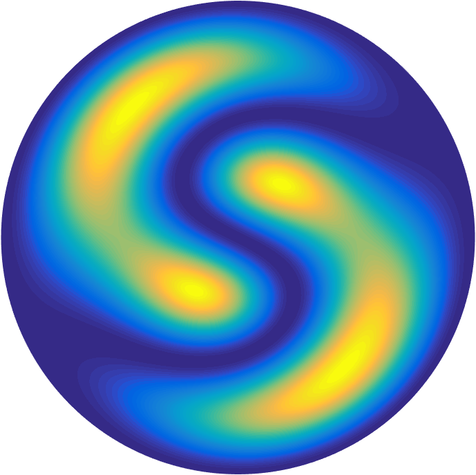
The example in Figure 4 illustrates the form of the final approximant. Each $c_{j}(\rho)$ defines a radial “slice” of the function, and each $r_{j}(\theta)$ defines a circular “slice”. To form these slices, the GE algorithm adaptively samples $\tilde{f}$ along a sparse collection of lines referred to as the skeleton, and constructs a rank $K$ approximant of the form of (8). In this process, only $K^{2}+K(m+n)$ samples are required to approximate $\tilde{f}$ to machine precision, as opposed to the $mn$ samples required for the tensor product. As depicted in Figure 4, the use of low rank methods effectively counters the overresolution issues associated with applying Chebyshev–Fourier tensor product grids on the disk.

For an approximation to a function $f$ on the disk to be continuous and differentiable at $\rho=0$, the following properties must hold for the Fourier expansion of $f$ given in (2):

• (i)

  $k$ is even $\implies\phi_{k}(\rho)$ is an even function,

• (ii)

  $k$ is odd $\implies\phi_{k}(\rho)$ is an odd function,

• (iii)

  $k\not=0$ $\implies\phi_{k}(0)=0$.

In this section we show that these parity properties can be naturally recovered for the BMC-II function $\tilde{f}$, and are preserved by the GE procedure depicted in Figure 3.

Let $\tilde{f}$ be a BMC function defined via functions $g$ and $h$ in (4). Let $f^{\textnormal{{\tiny+}}}=g+h$ and $f^{\textnormal{{\tiny--}}}=g-h$. Then, $\tilde{f}$ can be written as a sum of two BMC functions [44, Section 3.2]:

i.e., $\tilde{f}=\frac{1}{2}(\tilde{f}^{\textnormal{{\tiny+}}}+\tilde{f}^{\textnormal{{\tiny--}}})$. From (16), we can deduce that $\tilde{f}^{\textnormal{{\tiny+}}}$ is an even function in $\rho$ and $\pi$-periodic in $\theta$, whereas $\tilde{f}^{\textnormal{{\tiny--}}}$ is an odd function in $\rho$ and $\pi$-antiperiodic in $\theta$. This is equivalent to the statement of parity properties (i) and (ii), as $\pi$-periodic functions have only even Fourier modes and $\pi$-antiperiodic functions have only odd Fourier modes. While many techniques enforce these parity-based restrictions on the Fourier and Chebyshev coefficients of functions on the disk, relating these properties more generally to BMC-II functions allows one to apply these restrictions directly through the values of a function, without ever using the coefficients. This is the premise our GE procedure operates on.

As shown in Section 3.2 of [44], we can write the GE step (14) as

where $m^{\textnormal{{\tiny+}}}$ and $m^{\textnormal{{\tiny--}}}$ are values⁴⁴ 4 Note that $m^{\textnormal{{\tiny+}}}$ and $m^{\textnormal{{\tiny--}}}$ are not related to $m$ in (3). derived from the spectral decomposition of $M^{\dagger_{\epsilon}}$, and are given by

Here, $0<\alpha<1$ is referred as the coupling parameter for the GE procedure, and $\alpha$ determines $\epsilon$ in $M^{\dagger_{\epsilon}}$: $\alpha=\epsilon/\sigma_{1}(M)=\epsilon/\max\{|a+b|,|a-b|\}$. The decomposition in (17) reveals an alternative interpretation of structure-preserving GE as a coupled process involving two standard GE procedures. If either of the first two cases of (18) is chosen, GE with complete pivoting is performed on only one term in (17), resulting in a rank 1 update. In the third case of (18), $M^{\dagger_{\epsilon}}=M^{-1}$, and a rank $2$ update is achieved. It is desirable to perform as many rank $2$ updates as possible, as this reduces the overall number of pivot searches required by the GE procedure. Too small a value of $\alpha$ may allow the use of $M^{-1}$ when it is ill–conditioned, but choosing $\alpha$ too close to $1$ hampers the efficiency of the procedure. We have experimented with several values for $\alpha$ and find that $\alpha=1/100$ works well in practice. The role of $\alpha$ in the convergence rate of the GE procedure is discussed further in Section 3.4.

Following [44], we can exploit (17) to write the low rank approximation to $\tilde{f}$ as

where $K^{\textnormal{{\tiny+}}}+K^{\textnormal{{\tiny--}}}=K$. Here, the functions ${c}^{\textnormal{{\tiny+}}}_{j}(\rho)$ and ${r}^{\textnormal{{\tiny+}}}_{j}(\theta)$ for $1\leq j\leq K^{\textnormal{{\tiny+}}}$ are even and $\pi$-periodic, respectively, while ${c}^{\textnormal{{\tiny--}}}_{j}(\rho)$ and ${r}^{\textnormal{{\tiny--}}}_{j}(\theta)$ for $1\leq j\leq K^{\textnormal{{\tiny--}}}$ are odd and $\pi$-antiperiodic, respectively. The pivots, $d^{\textnormal{{\tiny+}}}$ and $d^{\textnormal{{\tiny--}}}$, are related to the $2\times 2$ pivot matrix given in (9) [44]. If $f$ is non-zero at the origin, the first step of the GE procedure is given by (15). This chooses ${c}^{\textnormal{{\tiny+}}}_{1}(\rho)=\tilde{f}(\theta^{*},\rho)$, ${r}^{\textnormal{{\tiny+}}}_{1}(\theta)=1$, and $d^{\textnormal{{\tiny+}}}_{1}=1$, so that for $j>1$, $c_{j}(0)=0$. Crucially, this ensures that parity property (iii) is preserved in the decomposition.

Using (19), the parity properties of $\tilde{f}$ are given explicitly, and this can be used to simplify algorithmic procedures. An example is given in Section 4.3 on integration. This expression also clarifies why our approximants are stable for differentiation (see Section 4.4).

In [44], it is shown that BMC structure-preserving GE exactly recovers BMC functions of finite rank. In this section, we prove that for certain analytic functions of infinite rank, structure-preserving GE converges at a geometric rate. Specifically, we will consider a function $\tilde{f}$ that is analytically continuable in at least one variable to a sufficiently large region of the complex plane.We characterize this region formally using the concept of a stadium.

To understand convergence, we will view structure-preserving GE as a coupled procedure involving the functions $\tilde{f^{\textnormal{{\tiny+}}}}$ and $\tilde{f^{\textnormal{{\tiny--}}}}$ defined in Section 3.3. The proof requires an examination of the error produced after applying the GE step (17), and we see in (18) that there are three cases to consider. Bounds on the error are intimately tied to the growth factors of the GE procedures that are applied to $\tilde{f^{\textnormal{{\tiny+}}}}$ and $\tilde{f^{\textnormal{{\tiny--}}}}$. The growth factors quantify the worst possible increase in the absolute maximum of the function after a rank one update. Geometric convergence can be proven if the size of the stadium in which $\tilde{f}$ is analytic is large enough to counteract the potential growth induced by GE.

The connection between the region of analyticity and the GE growth factor is made clear in the proof of Theorem $8.1$ in [43], which shows that iterative GE with complete pivoting as in (7) converges geometrically for functions that are analytic within a sufficiently large stadium. In the first or second case of (18), standard GE with complete pivoting is applied to either $\tilde{f}^{\textnormal{{\tiny+}}}$ or $\tilde{f}^{\textnormal{{\tiny--}}}$, and we may use Theorem $8.1$ directly. In the third case of (18), two GE procedures are performed: a GE step with complete pivoting is applied to whichever of the two functions $\tilde{f}^{\textnormal{{\tiny+}}}$ or $\tilde{f}^{\textnormal{{\tiny--}}}$ has a larger absolute maximum value, and a GE step with a nonstandard pivoting strategy is applied to the other function. If a bound on the growth factor of this nonstandard GE step is known, then as long as $\tilde{f}$ is assumed to be analytic in an appropriately-sized region of the complex plane, we can apply a mild generalization of Theorem 8.1. For this reason, we require the following lemma associated with the third case of (18):

Since bounds on the growth factors are known for each GE procedure applied on $\tilde{f}^{\textnormal{{\tiny+}}}$ and $\tilde{f}^{\textnormal{{\tiny--}}}$, geometric convergence of the BMC structure-preserving GE can now be proven. A theorem analogous to the one below holds with the roles of $\theta$ and $\rho$ exchanged.

The assumptions required on $\tilde{f}$ in Theorem 5 are rather restrictive, as the proof of convergence requires us to consider GE growth rates that account for the worst-case scenario. Empirically, we observe convergence for a much broader class of functions, and at rates that are asymptotically optimal. This is described in the next section.

While Section 3.4 proves that convergence of the GE procedure in Figure 3 is geometric when $f$ is analytic in a sufficiently large region of the complex plane, we observe in practice that the procedure converges at near-optimal rates for functions that are only a few times differentiable.

If $\tilde{f}$ is Lipschitz continuous with respect to both variables for $(\theta,\rho)\in[-\pi,\pi]\times[-1,1]$, then the best rank $K$ approximation to $\tilde{f}$ is given by the Karhunen-Loève expansion, also called the the singular value decomposition (SVD), of $\tilde{f}$:

The non-increasing sequence $\sigma_{1}\geq\sigma_{2}\geq\cdots$ of real, nonnegative numbers are the singular values of $\tilde{f}$. The continuous singular functions $\{u_{j}(\rho)\}$ and $\{v_{j}(\theta)\}$ each form an orthonormal set of functions with respect to the standard $L_{2}$ inner product. A best rank $K$ approximation to $\tilde{f}$, in the sense of the $L_{2}$ norm, is constructed by truncating (24) after $K$ terms [35].

For reasons closely related to those discussed in Section 3.3, the SVD preserves the BMC structure of $\tilde{f}$ [49]. Unfortunately, the high cost of computing the SVD makes this an untenable approach for constructing low rank approximants to $\tilde{f}$ in practice.

Nonetheless, approximants constructed via the SVD are optimal with respect to $\|\cdot\|_{2}$, and this provides a way to check the quality of the low rank approximants constructed by our GE procedure. Figure 5 displays the $L_{2}$ error over $[-\pi,\pi]\times[-1,1]$ for rank $K$ approximations constructed via the SVD and the GE procedure for the following two BMC-II functions:

where $\omega(\theta,\rho)=\left((\rho\cos\theta-.2)^{2}+(\rho\sin\theta-.2)^{2}\right)^{1/2}$ and $\zeta_{\textnormal{{\tiny+}}}=\max\{\zeta,0\}$. The error given by the SVD behaves in accordance with known theoretical results, decaying geometrically for the function $\phi_{1}$ and at an algebraic rate for $\phi_{2}$ [39]. In experiments, it is observed that our GE procedure constructs near-best low rank approximants to smooth BMC functions.

References

- [1] P. Amore, Solving the Helmholtz equation for membranes of arbitrary shape: numerical results, J. of Phys. A: Mathematical and Theoretical, 41 (2008), pp. 265–206.
- [2] M. Bebendorf, Approximation of boundary element matrices, Numer. Math., 86 (2000), pp. 565–589.
- [3] B. Beckermann and A. Townsend, On the singular values of matrices with displacement structure, SIAM J. Matrix Anal. Appl., (2016). To appear.
- [4] P. Benner, R.-C. Li, and N. Truhar, On the ADI method for Sylvester equations, J. Comput. Appl. Math., 233 (2009), pp. 1035–1045.
- [5] A. Bhatia and E. Wolf, On the circle polynomials of Zernike and related orthogonal sets, in Mathematical Proceedings of the Cambridge Philosophical Society, vol. 50, Cambridge Univ Press, 1954, pp. 40–48.
- [6] J. P. Boyd, Chebyshev and Fourier Spectral Methods, Courier Corporation, 2001.
- [7] J. P. Boyd and F. Yu, Comparing seven spectral methods for interpolation and for solving the Poisson equation in a disk: Zernike polynomials, Logan–Shepp ridge polynomials, Chebyshev–Fourier series, cylindrical Robert functions, Bessel–Fourier expansions, square-to-disk conformal mapping and radial basis functions, J. Comput. Phys., 230 (2011), pp. 1408–1438.
- [8] O. A. Carvajal, F. W. Chapman, and K. O. Geddes, Hybrid symbolic-numeric integration in multiple dimensions via tensor-product series, in Proceedings of the 2005 international symposium on symbolic and algebraic computation, ACM, 2005, pp. 84–91.
- [9] R. Churchill, Fourier Series and Boundary Value Problems, McGraw-Hill book Company, Incorporated, 1941.
- [10] T. A. Driscoll, N. Hale, and L. N. Trefethen, eds., Chebfun Guide, Pafnuty Publications, Oxford, 2014.
- [11] H. Eisen, W. Heinrichs, and K. Witsch, Spectral collocation methods and polar coordinate singularities, J. Comput. Phys., 96 (1991), pp. 241–257.
- [12] B. Fornberg, A pseudospectral approach for polar and spherical geometries, SIAM J. Sci. Comp., 16 (1995), pp. 1071–1081.
- [13] B. Fornberg and N. Flyer, A Primer on Radial Basis Functions with Applications to the Geosciences, SIAM, Philadelphia, 2015.
- [14] L. V. Foster and X. Liu, Comparison of rank revealing algorithms applied to matrices with well defined numerical ranks, 2006.
- [15] P. Godon, Numerical modeling of tidal effects in polytropic accretion disks, The Astrophysical Journal, 480 (1997), p. 329.
- [16] G. H. Golub and C. F. Van Loan, Matrix Computations, Johns Hopkins University Press, 2012. 4th edition.
- [17] S. A. Goreinov, E. E. Tyrtyshnikov, and N. L. Zamarashkin, A theory of pseudoskeleton approximations, Linear Algebra and its Applications, 261 (1997), pp. 1–21.
- [18] N. Halko, P.-G. Martinsson, and J. A. Tropp, Finding structure with randomness: Probabilistic algorithms for constructing approximate matrix decompositions, SIAM review, 53 (2011), pp. 217–288.
- [19] W. Heinrichs, Spectral collocation schemes on the unit disc, J. Comput. Phys., 199 (2004), pp. 66–86.
- [20] A. R. H. Heryudono and T. A. Driscoll, Radial basis function interpolation on irregular domains through conformal transplantation, J. Sci. Comput., 44 (2010), pp. 286–300.
- [21] S. Kapurl, An algorithm for the fast Hankel transform, 1995. Yale technical report.
- [22] A. Karageorghis, C. Chen, and Y.-S. Smyrlis, A matrix decomposition RBF algorithm: Approximation of functions and their derivatives, Appl. Numer. Math., 57 (2007), pp. 304–319.
- [23] R. Kerswell, Recent progress in understanding the transition to turbulence in a pipe, Nonlinearity, 18 (2005), p. R17.
- [24] J.-R. Li and J. White, Low rank solution of Lyapunov equations, SIAM J. Matrix Anal. Appl., 24 (2002), pp. 260–280.
- [25] A. Lu and E. L. Wachspress, Solution of Lyapunov equations by alternating direction implicit iteration, Comp. & Math. with Appl., 21 (1991), pp. 43–58.
- [26] V. N. Mahajan and G. Dai, Orthonormal polynomials in wavefront analysis: analytical solution, JOSA A, 24 (2007), pp. 2994–3016.
- [27] G. Martin, Transformation Geometry: An Introduction to Symmetry, Springer, New York, 2012.
- [28] J. C. Mason and D. C. Handscomb, Chebyshev Polynomials, CRC Press, 2002.
- [29] P. E. Merilees, The pseudospectral approximation applied to the shallow water equations on a sphere, Atmosphere, 11 (1973), pp. 13–20.
- [30] F. W. Olver, D. W. Lozier, R. F. Boisver, and C. W. Clark, NIST Handbook of Mathematical Functions, Cambridge University Press, 2010.
- [31] S. Olver and A. Townsend, A fast and well-conditioned spectral method, SIAM Review, 55 (2013), pp. 462–489.
- [32] M. O’Neil, F. Woolfe, and V. Rokhlin, An algorithm for the rapid evaluation of special function transforms, App. Comp. Harm. Analy., 28 (2010), pp. 203–226.
- [33] J. Pringle, Accretion discs in astrophysics, Annual Review of Astronomy and Astrophysics, 19 (1981), pp. 137–162.
- [34] J. Sabino, Solution of large-scale Lyapunov equations via the block modified Smith method, PhD thesis, Rice University, 2006.
- [35] E. Schmidt, Zur Theorie der linearen und nichtlinearen Integralgleichungen. iii. Teil, Mathematische Annalen, 65 (1908), pp. 370–399.
- [36] H. A. Schwarz, Ueber einige Abbildungsaufgaben, Journal für die reine und angewandte Mathematik, 70 (1869), pp. 105–120.
- [37] E. Serre and J. Pulicani, A three-dimensional pseudospectral method for rotating flows in a cylinder, Computers and Fluids, 30 (2001), pp. 491–519.
- [38] J. Shen, A new fast Chebyshev–Fourier algorithm for Poisson-type equations in polar geometries, Appl. Numer. Math., 33 (2000), pp. 183–190.
- [39] A. Townsend, Computing with functions in two dimensions, PhD thesis, University of Oxford, 2014.
- [40] , A fast analysis-based discrete Hankel transform using asymptotic expansions, SIAM J. Numer. Anal., 53 (2015), pp. 1897–1917.
- [41] , Gaussian elimination corrects pivoting mistakes, arXiv preprint arXiv:1602.06602, (2016).
- [42] A. Townsend and L. N. Trefethen, An extension of Chebfun to two dimensions, SIAM J. Sci. Comp., 35 (2013), pp. C495–C518.
- [43] , Continuous analogues of matrix factorizations, in Proc. Royal Soc. A, vol. 471, 2015, pp. 1–21.
- [44] A. Townsend, H. Wilber, and G. B. Wright, Computing with functions in spherical and polar geometries I. The sphere, SIAM J. Sci. Comp., 38-4 (2016), pp. C403–C425.
- [45] L. N. Trefethen, Spectral Methods in MATLAB, SIAM, 2000.
- [46] , Householder triangularization of a quasimatrix, IMA J. Numer. Anal., (2009), p. drp018.
- [47] , Approximation Theory and Approximation Practice, SIAM, 2013.
- [48] G. M. Vasil, K. J. Burns, D. Lecoanet, S. Olver, B. P. Brown, and J. S. Oishi, Tensor calculus in polar coordinates using jacobi polynomials, J. Comput. Phys., 325 (2016), pp. 53–73.
- [49] H. Wilber, Numerical computing with functions on the sphere and disk, Master’s thesis, Boise State University, 2016.
- [50] G. B. Wright, M. Javed, H. Montanelli, and L. N. Trefethen, Extension of Chebfun to periodic functions, SIAM J. Sci. Comp., 37 (2015), pp. C554–C573.
- [51] F. Zernike, Beugungstheorie des schneidenver fahrens und seiner verbesserten form, der phasenkontrastmethode, Physica, 1 (1934), pp. 689–704.