Tautochrone and Brachistochrone Shape Solutions for Rocking Rigid Bodies
Abstract
Rocking rigid bodies appear in several shapes in everyday life: As furniture like rocking chairs and rocking cradles or as toys like rocking horses or tilting dolls. The familiar rocking motion of these objects, a non-linear combination of a rigid rotation and a translation of the center of mass, gives rise to a number of interesting dynamical properties. However, their study has received little attention in the literature.
This work presents a comprehensive introduction to the dynamics of rocking rigid bodies, including a concise derivation of the equations of motion as well as a general inversion procedure to construct rocking rigid body shapes with specified dynamical properties. Moreover, two novel rigid body shapes are derived — the tautochrone shape and the brachistochrone shape — which represent an intriguing generalization of the well-know tautochrone and brachistochrone curves. In particular, tautochrone shapes offer an alternative construction of a tautochrone pendulum, in addition to Huygens’ cycloid pendulum solution.
Key words: rigid body – tautochrone – isochrone – brachistochrone – rocking motion – rolling without slip
1 Introduction
Rocking rigid bodies exhibit a rich dynamic behavior: They rock and roll, slide or tumble over and might deadlock at concave boundary sections. The governing equations of motion are strongly non-linear, such that their study requires numerical studies or semi-analytical techniques. As such, they have been widely studied in the field of earth quake safety analysis [3, 16, 15, 22, 26, 28]. In addition, detailed studies of static equilibria of balanced rigid bodies established close relations to geometrical and topological theorems [8]. The quest for minimizing the number of equilibrium points resulted in the discovery of the Gömböc, a remarkable three-dimensional shape featuring only one stable and one unstable equilibrium [27]. Despite these diverse research approaches there are two classical mechanics problems which have not been applied to rocking rigid bodies yet: the tautochrone11 1 From Ancient Greek, meaning “same time”. “isochrone” is in use as well. problem and the brachistochrone22 2 From Ancient Greek, meaning “shortest time”. problem. The tautochrone problem asks for the path along which a frictionless gliding bead returns in constant time to a fixed reference position, independent of the starting point on that path. Christiaan Huygens already found in 1660 the solution for a bead moving in the homogeneous gravity field of the earth: the inverted cycloid [9]. The brachistochrone problem asks for the path along which a frictionless bead slides from a given starting point to a given end point in minimum time. Though both problems seem to be unrelated, Johann Bernoulli discovered later in 1697 that the brachistochrone curve in an homogeneous gravity field is given by the same inverted cycloid33 3 The coincidence of tautochrone and brachistochrone paths does not apply to all potentials, see [7] for a detailed account.. As the calculation of the brachistochrone path requires the minimization of an integral, it also initiated a whole new field, the calculus of variations, and has seen many generalizations since. Quickest paths of descent have been derived for other potentials, geometries, curved space-time and various frictional forces [12, 17, 19, 20, 24, 25]. The tautochrone problem has seen similar generalizations as well [11, 18, 21].
As none of these generalizations covers rocking rigid bodies, let me begin with a close adaptation of both problems to planar (i.e. slab-like) rocking rigid bodies:
- •
A rocking rigid body is said to have a tautochrone shape if it returns to its equilibrium position in constant time.
- •
A rocking rigid body is said to have a brachistochrone shape if it returns from a given initial orientation to its equilibrium position in minimal time.
Having stated the problems to be solved, the remainder of the paper addresses the derivation of both novel shape solutions. The account starts with an introduction to rocking rigid body dynamics using complex calculus, followed by a generic inversion procedure to derive rigid body shapes from any desired rocking characteristics. Then both shapes solutions are derived, including a brief analysis of the balance of frictional forces at the contact point to explore the actual construction of these shapes.
2 Rocking Rigid Bodies

The study of a rocking rigid body requires an accurate description of the rigid body and its dynamics. It is customary to use two coordinate systems: A body-fixed coordinate system (, in the following) and a space-fixed coordinate system (, in the following). The body rolls along a rigid support plane defined at . Without loss of generality, the body-fixed coordinate system is defined such that it coincides with the space-fixed coordinate system when the rigid body assumes some (preferably stable) equilibrium position. In particular, the origin is chosen such that it coincides with the corresponding equilibrium contact point.
The mass distribution of a rigid body is sufficiently described by its moment of inertia and the position of its center of mass, located at owing to the definition of the body-fixed coordinate system. For the time being, I will assume a rocking motion without slip. In virtue of that assumption, any rotation by an angle (measured in clockwise direction) induces a translation in -direction. is defined as the unrolled curve length of the body contour measured from the origin to the contact point . and are related to the local radius of curvature by
| (1) |
Negative radii correspond to a “hanging” rigid body, that is the rigid body rolls along the underside of the support plane. The contour traced out by all contact points is the shape function of the rigid body, or simply its shape. Fig. 1 summarizes all introduced variables and coordinate systems. The transformation from body-fixed coordinates to space-fixed coordinates is given by
Though only convex rigid bodies are actually capable of rolling along a planar surface, Eq. 2 extends the notion of “rolling” to any shape function where is a continuous function on the curve. Interestingly, this condition does not imply that a shape function needs to be differentiable everywhere. For instance, a figure-3 shaped curve is not differentiable at the join of the two arcs, yet a rolling procedure according to Eq. 2 is still well defined. The rolling motion of a rigid body is a special case of a much more general geometrically operation know as roulette [4]. A roulette is defined as the curve traced out by a reference point attached to a curve which rolls along a second, fixed reference curve.
Having thus established a generalized definition of rolling, it is worth to have a closer look at the parametrization of the rocking motion itself. The orientation of the rigid body might either be parametrized by the rocking angle , the unrolled curve length or the height of the center of mass . However, none of these parameters is guaranteed to uniquely parameterize the rocking motion, as they are generally related by multi-valued functions. Therefore a careful restriction of the parameter domains is required to obtain meaningful results for the problem at hand.
Using Eq. 2 to calculate the center of mass path in space-fixed coordinates gives
As refers exclusively to the contact point in the following, the subscript is dropped from now for brevity. The transformation described by Eqs. 2–2 suggests the introduction of complex coordinates44 4 Another interesting application is to express the rocking angle as a complex number to solve the equations of motion, see [25] for details. , to simplify the center of mass equation to
| (25) | |||||
| (26) | |||||
| (27) |
is the center of mass position measured relative to the contact point. Using the notion introduced above, the center of mass path is the roulette generated by the support plane, the shape function and the center of mass. For a better overview, Table 1 contains a summary of the used variables.
Useful is the relation
| (28) | |||||
| (29) |
which demonstrates that the contact point is the instantaneous center of rotation. By considering the imaginary part only it follows that
| (30) | |||||
| (31) |
which can be rearranged to provide an alternative expression for the local radius of curvature:
| (32) |
Finally, by using the real part of Eq. 29 we obtain a differential equation for the path of the center of mass in space-fixed coordinates:
| (33) |
The general analysis itself presented in this section allows for many interesting applications. As the primary focus of this work is a study of tautochrone and brachistochrone shapes, an illustrative example using conic sections can be found in Appendix A.
| body-fixed | space-fixed | comoving | |
|---|---|---|---|
| Center of mass | |||
| Contact point | 0 |
3 Static Equilibrium
A rocking solid in static equilibrium does not experience a net torque. This requires the center of mass to be vertically aligned with the contact point and holds. For smooth shapes this is equivalent to
| (34) |
Furthermore, following from Eq. 31, equilibrium points are always stationary points of the distance from the center of mass to the contact point. Planar rigid bodies of finite extend have at least one stable and one unstable equilibrium point, which is a direct consequence of the maximum-minimum theorem. Bodies with only one stable equilibrium are called monostatic, while the special case of one stable and one unstable equilibrium is denoted as mono-monostatic. A monostatic body is quite easily constructed, unless its mass distribution is required to be homogeneous. It can be shown that two-dimensional homogeneous monostatic bodies do not exist, which is equivalent to the famous Four-Vertex theorem [27].
Differentiating Eq. 34 with respect to provides further insight into the type of equilibrium. The derivative is
| (35) |
which proves the following physical classification of equilibria:
- •
An equilibrium is stable if the center of mass is located below the local center of curvature
- •
An equilibrium is neutral if the center of mass coincides with the local center of curvature
- •
An equilibrium is unstable if the center of mass is located above the local center of curvature
These conditions apply equally well to negative radii of curvature, though this requires a generalized rocking motion in the sense of Eq. 2.
4 Equations of Motion
The motion of a rocking body combines a translation of the center of mass with a rotational motion in the gravity field of the earth. Thus the Lagrangian (normalized by the mass of the rigid body) reads
| (36) |
where dots indicate the derivative with respect to time. is the normalized moment of inertia (equal to the squared radius of gyration) and is the gravitational acceleration of the earth. In virtue of the no-slip assumption, both and can be considered as functions of only which further simplifies the Lagrangian to:
| (37) |
The Euler-Lagrange equation of motion is:
| (38) |
Before examining the exact solution of Eq. 38, it is useful to consider the small angle approximation
| (39) |
This is the differential equation of an harmonic oscillator with frequency
| (40) |
For later use, it is convenient to introduce the half-length of a pendulum with frequency :
| (41) |
To solve the full equation of motion, I introduce a new auxiliary parameter
| (42) |
which simplifies the Lagrangian and the equation of motion to:
| (43) | |||||
| (44) |
Hence the dynamics of a rocking rigid body is equivalent to a point mass moving in an effective potential . Eq. 44 can be solved by invoking the conservation of energy:
| (45) |
sets the maximal amplitude of the rocking motion.
5 Constraint Force
The weight of the rocking rigid body as well as the dynamic forces due to the rocking motion need to be balanced by the support plane. Therefore the constraint acceleration acting on the contact point is
| (46) |
Applying Eq. 29 twice provides the velocity and acceleration of the center of mass:
| (47) | |||||
| (48) |
Inserting Eq. 38 gives the desired acceleration
| (49) |
6 Inverse Problem
A vital problem in the analysis of rocking rigid bodies is the reconstruction of a valid shape function from a desired effective potential. Solving this inverse problem is not only a major step towards the calculation of tautochrone shapes (see next section), but also a general tool to create rocking rigid bodies with tailor-made dynamical properties.
To begin with, I restate the definition of the effective potential
| (50) |
where the potential is normalized such that holds for convenience. Instead of a result, is now considered as a free function and the shape function (or equivalently or ) is solved for. Applying the inverse potential function and deriving both sides of the equation with respect to yields
| (51) |
is an auxiliary function which maps the effective potential to its corresponding gradient:
| (52) |
In the most general case, is a multi-valued function which requires a separate inversion for each branch and a careful assembly of these solutions into one or multiple global shapes. Therefore I assume a symmetric effective potential with only on minimum at in the following to reduce the calculation down to a single (e.g. ) branch. Eq. 51 is an implicit equation for which can be directly solved for
| (53) |
thus providing the solution parametrized as . Alternatively, depending on , some other parametrization might be more suitable. It remains to calculate the shape function . Rearranging Eq. 25 suggests the Ansatz:
| (54) |
Re-inserting this Ansatz into Eq. 25 provides the required differential equations for and :
| (55) | |||||
| (56) |
Both equations are manifestly invariant under change of parametrization.
7 Tautochrone Shape
To solve the tautochrone shape problem, it is left to apply the inversion procedure from the previous section to an isochronous effective potential . It is tempting to assume that only harmonic potentials are isochrone potentials. But, in fact, the harmonic potential is only one solution among many other isochronous potentials. Only if the solution space is restricted to symmetric potentials it stands out as the sole solution [5]. Therefore I restrict the sought isochronous shapes to symmetric solutions only and continue with the harmonic potential:

| (57) | |||||
| (58) |
needs to be consistent with the small angle approximation. Hence is identical to the frequency defined by Eq. 40. Inserting Eq. 58 into Eq. 53 gives
| (59) |
By construction, the solution of the auxiliary parameter is
| (60) |
The right hand side of Eq. 59 needs to be positive, thus the valid range of is restricted to the interval . Likewise, is bounded by . This motivates to use as the scale length of the problem at hand and to switch to a dimensionless set of parameters [6]:
| (61) | |||||
| (62) | |||||
| (63) |
The tautochrone shape solution is monostatic by construction. Thus it is possible to parametrize the shape function by , though the domain of needs to be restricted to (there is a symmetric branch for ). All previously introduced parameters are readily expressed as dimensionless quantities:
| (64) | |||||
| (65) | |||||
| (66) |
The tilde is a short-hand notation for the normalization by an appropriated power of (e.g. ). Rewriting Eq. 59 using normalized quantities reads
| (67) |
Now all tools are in place for a detailed discussion of the properties of the tautochrone shape solution. It is important to note that some tautochrone shapes actually “roll” along the underside of the support plane, which is true for (i.e. ). For completeness, this special case is discussed in Appendix B.

7.1 Shape Function
The rocking angle is obtained by solving the differential equation 55 with initial condition :
| (68) |
In general, this integral can only be solved by means of elliptic integrals and is not representable by elementary functions. Nonetheless, it is possible to obtain valuable insight into the characteristics of the resulting shape function by examining the local radius of curvature (recall Eq. 32)
| (69) |
is a simple monotonously increasing function assuming infinity at . Thus asymptotically approaches a straight line for . The asymptote is readily obtained by formally expanding at :
| (70) | |||||
| (71) |
An alternative representation of the asymptote is
| (72) |
Fig. 2 illustrates this transition from a circular arc of radius into a straight line running to infinity, which is a characteristic of all tautochrone shapes. is directly related to the winding number defined with respect to the center of mass. Large values result in self-intersecting shape functions. Though these self-intersections do not pose any mathematical problem, they are a key challenge when actually building real solids representing these solutions. It is possible to study some properties of by considering special cases in the parameter space. At , can be expressed by elementary functions:
| (73) |
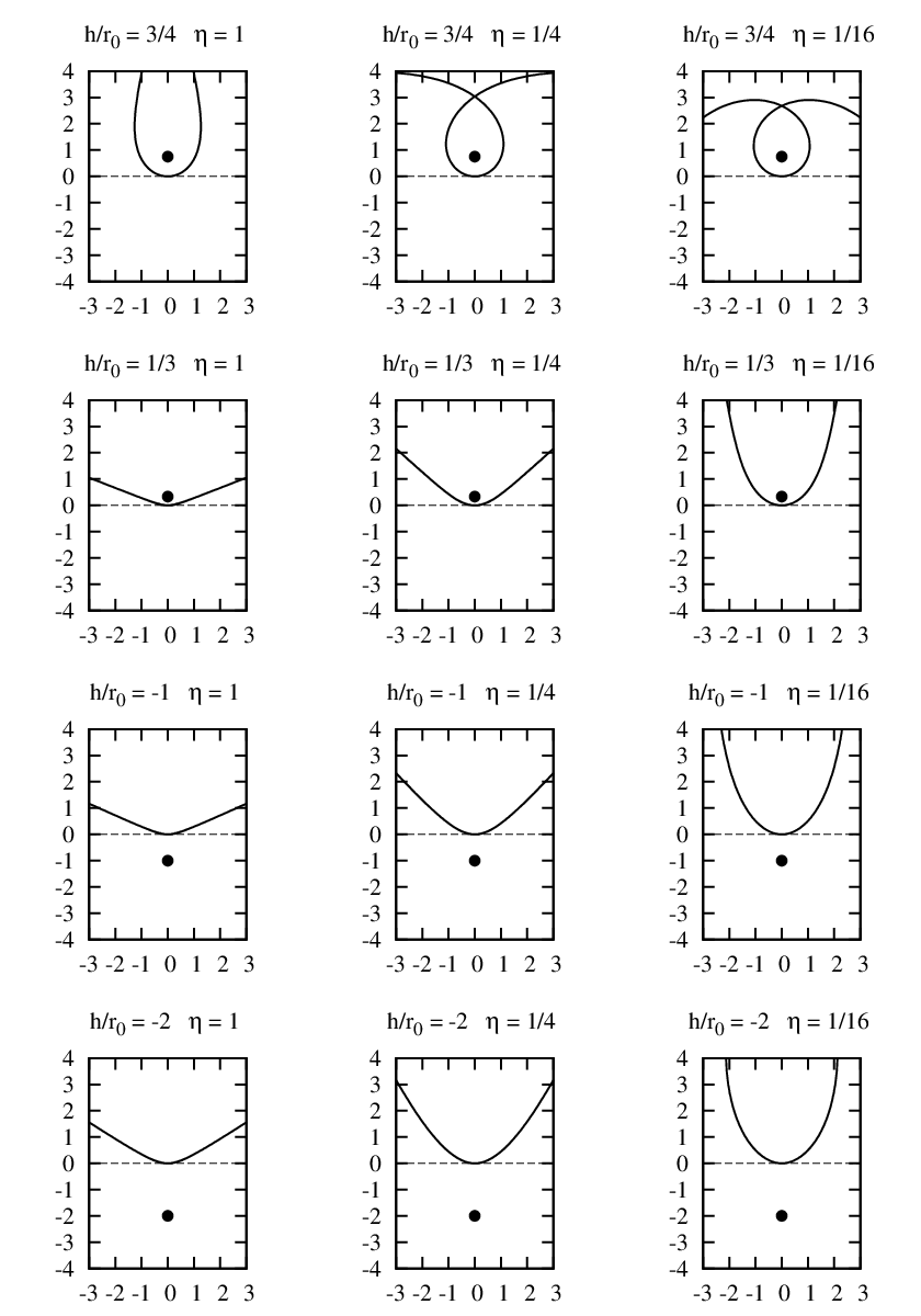
As approaches , the shape function winds ever tighter around the center of mass. On the contrary, this is not true for (i.e. the rocking pendulum limit). The rocking angle is bound by in this case. Small values of permit the approximation
| (74) | |||||
| (75) |
is the complete elliptic integral of the first kind [1]. is an overall good indicator of the winding number of a shape solution. A compilation of solutions in Fig. 4 illustrates the trend towards larger winding numbers as this parameter increases. The two center rows corresponding to further underline this finding. Though the center of mass is located once above and once below the supporting plane, both sets of tautochrone shapes are remarkably similar.
In particular intriguing is the limit . At first, it seems that a well defined limit does not exist, as the rocking angle integral diverges. However, it is possible to introduce as a free parameter to obtain a well defined family of solutions:
| (76) | |||||
| (77) |
Since holds in this limit as well, drops out of Eq. 29 and the center of mass moves independently from on the same path. Fig. 3 illustrates the solution for . Close to the origin the rocking angle varies as which is a general Archimedean spiral with exponent . The next section proves another fascinating property: The center of mass moves along a cylcoid when unrolling this curve.
7.2 Center of Mass
The tautochrone center of mass path is the solution of the differential equation
| (78) |
As for the rocking angle, the most general solution needs to be expressed in terms of elliptic integrals. An inspection of the right hand side provides the bound for all admissible values of . Further insight might be obtained by considering the case of a vanishing moment of inertia , which implies either , or . With all the mass concentrated in a single point, the rocking rigid body is equivalent to a point mass moving along a fixed path and the solution should be identical to the classical tautochrone. Indeed, formally solving Eq. 78 at recovers the well known inverted cycloid:
| (79) | |||||
| (80) | |||||
| (81) | |||||
| (82) |
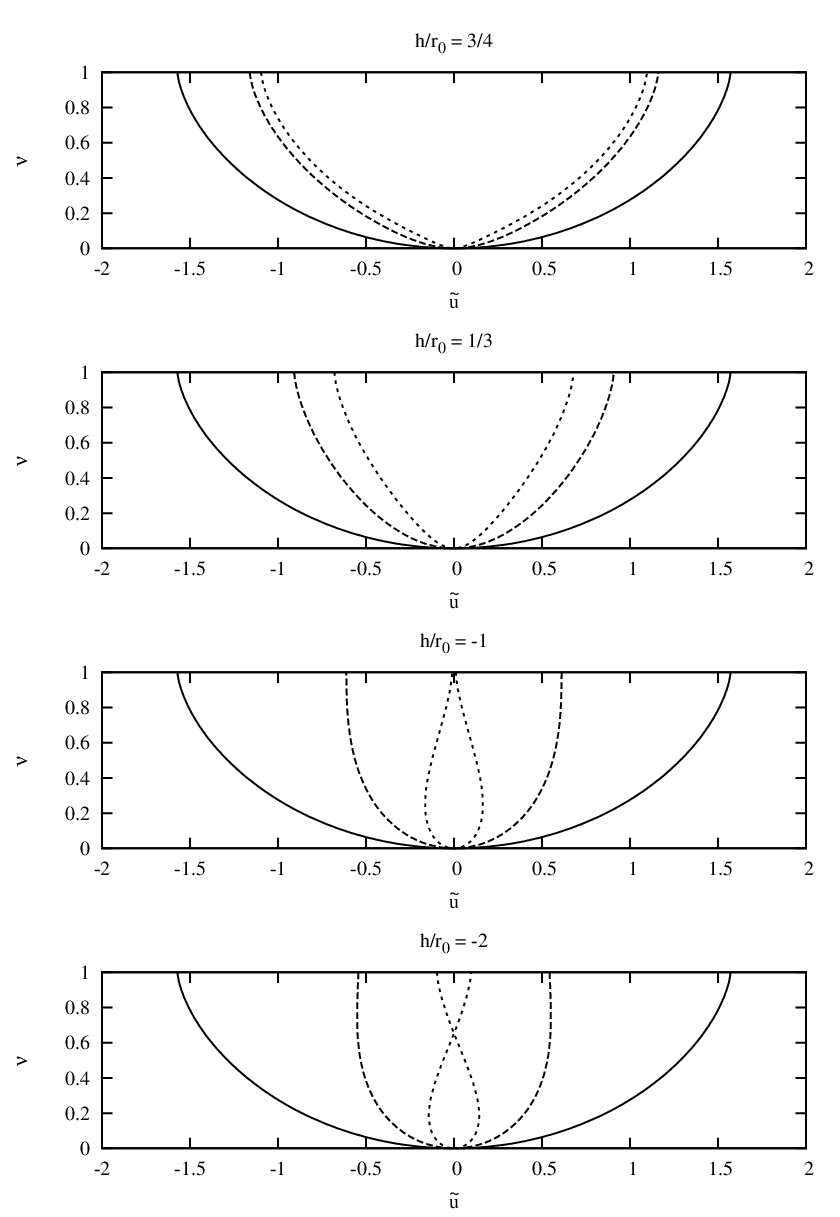
The cycloid parameter has a simple interpretation for maximal rocking amplitude . By considering the corresponding solution of the auxiliary parameter
| (83) |
the cycloid parameter is identified as being proportional to the elapsed time: . Though other parameter values do not allow for an elementary analytical solution, most center of mass paths still resemble a squeezed version of the inverted cycloid, as illustrated by selected center of mass paths in Fig. 5. Whenever the center of mass crosses the support plane, changes its sign and the center of mass pass path bends inwards, eventually leading to a self-intersection (see Fig. 5, lower panels).
8 Slipping
The analysis assumed so far a perfect rolling motion without any slipping. Though this is appropriate for a theoretical study, real bodies might in fact slip or even lift of the support plane [14]. A common physical model is to employ the static friction coefficient to formulate a physical no-slip condition based on the constraint acceleration acting at the contact point:
| (84) |
is the component parallel to the support plane, is the perpendicular component and is the static friction coefficient. In fact, Eq. 84 precludes jumps as well since an upward acceleration implies negative values of . Inserting the tautochrone solution into the expressions obtained in Section 5 gives
| (85) | |||||
| (86) |
By invoking the conversation of energy again, can be expressed as
| (87) |
which simplifies the constraint acceleration to
| (88) | |||||
| (89) |
is always positive, therefore tautochrone shapes are not subjected to jumping for all admissible values of . The constraint acceleration is both a function of and . Thus the no-slip condition needs to be validated for the entire rocking motion . This defines the set of rocking amplitudes which preclude slipping:
| (90) |
The upper bound is of particular interest, as it defines the range of the shape function that is accessible by a physical rocking motion. In general, Eq. 90 does not admit a simple closed-form solution for . However, imposing simplifies Eq. 90 to
| (91) |

This expression can be further reduced to a concise analytical solution
| (92) |
Though this solution is only strictly valid for , the general trend applies to other values of as well: Larger values of the friction coefficient allow the rigid body to explore a larger range of its shape function. However, does not provide an immediate indication as to what range of the shape function is accessible. All tautochrone shapes are well approximated by a circular arc for sufficiently small values of . The practical relevance of the derived tautochrone shapes is therefore characterized best by considering the ratio , which quantifies the maximal deviation from a simple circular shape. Making use of Eq. 69 provides the equation
| (93) |
Neglecting the dependence on , this equation favors small values of and . This trend can be further substantiated by numerically solving Eq. 90 for selected values of . Fig. 6 presents two choices, one being , a value not uncommon for most everyday materials like wood or plastic [23], and a second choice which requires more sticky surfaces like rubber. Results clearly favor large values, though viable regions in the parameter space still exist for .
9 Brachistochrone Shape
A brachistochrone shape minimizes the time required to roll from a given starting position back into its equilibrium position. Using the previously introduced notation is defined as
| (94) | |||||
| (95) |
where sets the initial rocking angle and the integration is performed over the branch. In agreement with the tautochrone problem, both the moment of inertia and the height of the center of mass are considered as fixed parameters. It is beneficial to change to as integration variable by employing Eq. 33:
| (96) |
Eq. 96 also provides a proper definition the ambiguous term “starting position” as the initial position of the center of mass in space-fixed coordinates. The integrand does not depend explicitly on , thus reducing the Euler-Lagrange equation to
| (97) |
where is a free integration constant carrying the same sign as . This equation can be solved for :
| (98) |
The corresponding solution is

| (99) |
The constant is determined by the boundary values of . By using the definition of the center of mass height , it is possible to obtain a more meaningful expression for :
| (100) |
is defined as in Eq. 62 and , in analogy to the tautochrone solution, is defined as
| (101) |
Employing both and simplifies Eq. 99 to
| (102) |
which is almost identical to the corresponding equation of the tautochrone shape (compare Eq. 59). However, the additional factor in Eq. 102 is only negligible in the limit , where the brachistochrone shape converges to the tautochrone shape solution. Finite values of require a much more careful analysis, and, as we will see, the resulting brachistochrone shapes are in remarkable contrast to the simplicity of the tautochrone solution. The first complication arises from the fact that the right hand side of Eq. 102 might become negative, and hence both and are undefined. Though this precludes the existence of a global minimizer of the variational problem, it is possible to join valid branches of the solution to obtain a minimizer on a reduced function space. Returning to the original variational Eq. 96 motivates to replace undefined values by for which the integrand assumes its minimum value. While this implies , this apparently strange result has a simple physical interpretation: The rigid body actually does not rotate at all but performs a free fall at velocity .
Another remarkable property stems from the fact that is singular at , implying that the brachistochrone shape decomposes into two separate parts. The rocking rigid body switches from one branch of the shape solution to another as the center of mass crosses the support plane.
Finally, calculating the local radius of curvature at the presumed equilibrium contact point gives
| (103) |
An inspection of reveals the somewhat disturbing property that the brachistochrone shape solution might violate the stability criterion . All these peculiarities can be consolidated by a detailed analysis of Eq. 102, which is presented in Appendix C for clarity. The result of this analysis is summarized best in the (, ) parameter plane (Fig. 7). The highlighted regions are:
- I)
The brachistochrone shape initially rolls along the support plane, followed by a free-fall down to . Though Eq. 103 technically violates the stability criterion in this case, this is only a mathematical artefact as the shape solution and therefore the local radius of curvature at is not defined.
- II)
The brachistochrone shape initially rolls along the support plane, performs an intermittent free-fall and continues the rolling motion on a second branch of the shape solution.
- III)
The local radius of curvature at is negative, thus indicating a rigid body rolling along the underside of the support plane.
- IV)
The center of mass crosses the support plane and switches over to a second branch of the shape solution.
Some of these regions partly overlap, which generates a rich variety of brachistochrone shape solutions. Sadly, this diversity largely represents extremely difficult-to-construct shape solutions, and only tautochrone-like shapes appear to be viable solutions.
10 Discussion
Rocking rigid bodies constitute an intriguing classical mechanics problem. This work presented a self-contained analysis of their dynamical properties, which can be applied to a broad range of rocking rigid bodies. In particular, this work focused on the derivation of two novel shape solutions: the tautochrone and the brachistochrone shape. Both shapes form a two-parametric family of solutions, parametrized by the center of mass height and the moment of inertia . By construction, tautochrone shapes exhibit a much more regular behavior than their brachistochrone counterparts. Moreover, tautochrone shapes offer a new alternative solution to Huygen’s cycloid approach to build an isochronous pendulum.
Although both the tautochrone and the brachistochrone shape are sufficiently described by this analysis, there remains an interesting challenge: Is it possible to demonstrate their properties by actually building physical representations of these shapes? A first analysis of the no-slip condition does not prohibit their construction, but the available parameter space is narrowed down to shapes with a comparably large moment of inertia (i.e. small values). In addition, both and are coupled through the mass distribution of the rigid body, which calls for an optimal design in terms of simplicity and elegance. This problem is left for future work.
Appendix A Illustrative Examples
An elegant set of rigid body shapes is obtained if the center of mass in comoving coordinates is required to move along a conic section with eccentricity . This Ansatz allows for a complete set of analytic solutions for , , and consequently . Furthermore, the center of mass moves along a conic section with eccentricity in space-fixed coordinates as well. Given and , two different solutions (either hyperbolas or ellipses) are obtained, parametrized by a suitably chosen parameter :
| for | ||
| for | ||
Shape solutions for are a sum of two counter-rotating logarithmic spirals, while shape solutions for are epicycloides and hypocycloids .

Appendix B Tautochrone Shape
All properties discussed in Section 7 apply equally well to tautochrone shape solutions with negative values of . In addition, the corresponding shape functions exhibit cusp-like features similar to epicycloids. This can be seen most easily by considering the tangent vector of the shape solution
| (104) |
The rocking angle is continuous and differentiable at . Hence the tangent vector abruptly inverts its direction at , leading to the cusps seen in Fig. 8 (right panel) and Fig. 9. The local radius of curvature vanishes at
| (105) |
A second interesting feature emerges when the center of mass may cross the support plane, which requires . By approximating at
| (106) | |||||
| (107) |
it is possible to derive an analytical solution for
| (108) | |||||
| (109) |
which is equivalent to the first example presented in Appendix A. In the limit both and tend to zero and the cusp turns into a joining point of two infinite, logarithmic spiral-like curves. However, the divergence is rather slow as the number of spiral revolutions is .

Appendix C Brachistochrone Shape
as defined by Eq. 102 might assume negative values, depending on and . To characterize the values () which lead to negative values, it is sufficient to study the roots of the polynomial
| (110) |
The roots of this quadratic polynomial are
| (111) |
At , evaluates to
| (112) | |||||
| (113) |
which is a positive quantity for all admissible values (). Therefore assumes negative values on the interval if and only if has at least one root in this interval. A necessary condition is that both roots are real, thus requiring
| (114) |
A detailed analysis of both roots provides the intervals
The intersection of both intervals, corresponding to a roll-drop-roll sequence, defines region II in Fig. 7, whereas region I corresponds to a single root and a roll-drop sequence.
References
- [1] M. Abramowitz and I. A. Stegun. Handbook of Mathematical Functions with Formulas, Graphs, and Mathematical Tables. Tenth Printing. New York: Dover, 1972.
- [2] C. Antón and J. L. Brun. Isochronous oscillations: Potentials derived from a parabola by shearing. American Journal of Physics, 76(6):537–540, 2008.
- [3] M. Aslam. Rocking and overturning response of rigid bodies to earthquake motions. Lawrence Berkeley National Laboratory, 2011.
- [4] William Henry Besant. Notes on Roulettes and Glissettes. Deighton, Bell, 1890.
- [5] S. Bolotin and R. S. MacKay. Isochronous potentials. Proceedings of the third conference: Localization and Energy Transfer in Nonlinear Systems, pages 217–224, 2003.
- [6] W. D. Curtis, J. David Logan, and W. A. Parker. Dimensional analysis and the pi theorem. Linear Algebra and its Applications, 47:117–126, 1982.
- [7] Harry H. Denman. Remarks on brachistochrone–tautochrone problems. American Journal of Physics, 53(3):224–227, 1985.
- [8] Gábor Domokos, András Árpád Sipos, and Tímea Szabó. The mechanics of rocking stones: equilibria on separated scales. Mathematical Geosciences, 44(1):71–89, 2012.
- [9] Alan Emmerson. Things are seldom what they seem – Christian Huygens, the pendulum and the cycloid. Horological Sci Newsl, 2005:2–32, 2005.
- [10] Herman Erlichson. Johann bernoulli’s brachistochrone solution using fermat’s principle of least time. European journal of physics, 20(5):299, 1999.
- [11] Eduardo Flores and Thomas J. Osler. The tautochrone under arbitrary potentials using fractional derivatives. American Journal of Physics, 67:718–722, 1999.
- [12] John Gemmer, R. Umble, and M. Nolan. Generalizations of the brachistochrone problem. arXiv preprint math-ph/0612052, 2006.
- [13] R. Gómez, V. Marquina, and S. Gómez-Aíza. An alternative solution to the general tautochrone problem. Revista mexicana de física E, 54(2):212–215, 2008.
- [14] Raul W. Gómez, J. J. Hernandez-Gomez, and Vivianne Marquina. A jumping cylinder on an inclined plane. European Journal of Physics, 33(5):1359, 2012.
- [15] Yuji Ishiyama. Motions of rigid bodies and criteria for overturning by earthquake excitations. Earthquake Engineering and Structural Dynamics, 10(5):635–650, 1982.
- [16] R. N. Iyengar and C. S. Manohar. Rocking response of rectangular rigid blocks under random noise base excitations. International journal of non-linear mechanics, 26(6):885–892, 1991.
- [17] O. Jeremić, S. Šalinić, A. Obradović, and Z. Mitrović. On the brachistochrone of a variable mass particle in general force fields. Mathematical and computer modelling, 54(11):2900–2912, 2011.
- [18] S. G. Kamath. Relativistic tautochrone. Journal of mathematical physics, 33(3):934–940, 1992.
- [19] V. P. Legeza. Brachistochrone for a rolling cylinder. Mechanics of solids, 45(1):27–33, 2010.
- [20] Stephan Mertens and Sebastian Mingramm. Brachistochrones with loose ends. European Journal of Physics, 29(6):1191, 2008.
- [21] R. Munoz and G. Fernández-Anaya. On a tautochrone-related family of paths. Revista mexicana de física E, 56(2):227–233, 2010.
- [22] Keisuke Nozaki, Yoshiaki Terumichi, Kazuhiko Nishimura, and Kiyoshi Sogabe. Study of rocking motion of rigid body with slide contact. Journal of mechanical science and technology, 23(4):1001–1007, 2009.
- [23] P. Onorato, M. Malgieri, P. Mascheretti, and A. De Ambrosis. Librational motion of asymmetric rolling bodies and the role of friction force. arXiv preprint arXiv:1410.6470, 2014.
- [24] A. S. Parnovsky. Some generalisations of brachistochrone problem. Acta Physica Polonica-Series A General Physics, 93:55–64, 1998.
- [25] Francisco Prieto and Paulo B. Lourenço. On the rocking behavior of rigid objects. Meccanica, 40(2):121–133, 2005.
- [26] H. Schau and M. Johannes. Rocking and sliding of unanchored bodies subjected to seismic load according to conventional and nuclear rules. In 4th ECCOMAS Thematic Conference on Computational Methods in Structural Dynamics and Earthquake Engineering (COMPDYN), 2013.
- [27] Péter L. Várkonyi and Gábor Domokos. Static equilibria of rigid bodies: dice, pebbles, and the poincaré-hopf theorem. Journal of Nonlinear Science, 16(3):255–281, 2006.
- [28] Tibor Winkler, Kimiro Meguro, and Fumio Yamazaki. Response of rigid body assemblies to dynamic excitation. Earthquake engineering & structural dynamics, 24(10):1389–1408, 1995.
*