TIT/HEP-653

UTHEP-684

On the mass-coupling relation of multi-scale quantum integrable models

Zoltán Bajnok Affiliation: MTA Lendület Holographic QFT Group, Wigner Research Centre
H-1525 Budapest 114, P.O.B. 49, Hungary Email: bajnok.zoltan@wigner.mta.hu János Balog Affiliation: MTA Lendület Holographic QFT Group, Wigner Research Centre
H-1525 Budapest 114, P.O.B. 49, Hungary Email: balog.janos@wigner.mta.hu Katsushi Ito Affiliation: Department of Physics, Tokyo Institute of Technology
Tokyo 152-8551, Japan Email: ito@th.phys.titech.ac.jp Yuji Satoh Affiliation: Institute of Physics, University of Tsukuba
Ibaraki 305-8571, Japan Email: ysatoh@het.ph.tsukuba.ac.jp and Gábor Zsolt Tóth Affiliation: MTA Lendület Holographic QFT Group, Wigner Research Centre
H-1525 Budapest 114, P.O.B. 49, Hungary Email: toth.gabor.zsolt@wigner.mta.hu

Abstract

We determine exactly the mass-coupling relation for the simplest multi-scale quantum integrable model, the homogenous sine-Gordon model with two independent mass-scales. We first reformulate its perturbed coset CFT description in terms of the perturbation of a projected product of minimal models. This representation enables us to identify conserved tensor currents on the UV side. These UV operators are then mapped via form factor perturbation theory to operators on the IR side, which are characterized by their form factors. The relation between the UV and IR operators is given in terms of the sought-for mass-coupling relation. By generalizing the $\Theta$ sum rule Ward identity we are able to derive differential equations for the mass-coupling relation, which we solve in terms of hypergeometric functions. We check these results against the data obtained by numerically solving the thermodynamic Bethe Ansatz equations, and find a complete agreement.

1 Introduction

There have been an increasing interest and relevant progress in studying $1+1$ dimensional integrable quantum field theories (QFTs), due to the fact that they can be solved exactly. The usual definitions of QFTs are based on a Lagrangian and the main¹¹ 1 Some non-perturbative methods exist especially for supersymmetric QFTs. analytical tool to investigate them is perturbation theory, which provides a systematic expansion of physical quantities around a properly chosen free theory. In general, only a few terms are calculable technically, leading to merely approximate results.

Integrable $1+1$ dimensional QFTs are special in the sense that they offer an exact non-perturbative treatment [1, 2]. Their exact bootstrap solution does not start from any Lagrangian, rather it determines the scattering matrices of the particles from such consistency requirements as unitarity and crossing symmetry assuming maximal analyticity. In contrast to the ultraviolet (UV) description based on the Lagrangian the infrared (IR) formulation relies on the particle masses and the scattering matrices. In the simplest case of the scaling Lee-Yang model there is only one type of particle with a given mass and the scattering matrix is a simple CDD factor without any parameter [3]. The procedure to connect the large scale IR scattering theory to a small scale UV Lagrangian formulation is to put the system in a finite size and calculate an interpolating quantity, such as the ground-state energy, exactly.

The Thermodynamic Bethe Ansatz (TBA) equation [4] describes the ground state energy from the IR side by summing up all the vacuum polarization effects. This is a nonlinear integral equation depending on the scattering matrix and the masses of the particles. Unfortunately the TBA equation does not allow any systematic analytic small volume expansion. Nevertheless, the central charge of the UV limiting theory and the bulk energy constant can be extracted exactly. The central charge basically identifies the UV conformal field theory (CFT), which is perturbed with relevant operators. Demanding the integrability of the perturbation leaves a few choices, from which the one matching with the IR description can be easily singled out. The identification between the UV perturbed CFT (pCFT) Lagrangian and the IR scattering theory boils down to the relation between the mass of the fundamental particle and the strength of the perturbation. This relation is called the mass-coupling relation and is a real challenge to calculate in any integrable model. This relation is of fundamental significance as it also gives the vacuum expectation values of the perturbing operators, which contain all the non-perturbative information which is not captured by the pCFT [5, 6].

In order to calculate the mass-coupling relation one typically embeds the theory into a larger model with extra symmetries. After introducing some type of magnetic field coupled to the extra conserved current the TBA equations can be linearized and expanded systematically. Comparing the result with the analogous perturbative expansion on the Lagrangian side the relation between the masses and the parameters of the Lagrangian can be established. This route was followed for the O(3) [7] and sine-Gordon models [8] and has been extended for many other integrable models [9, 10, 11, 12, 13, 14, 15, 16, 17]. (For a different route, see [18].) None of these models, however, contains integrable perturbations with more than one mass scale. Even though the models have multi-parameters and/or a non-trivial spectrum, the mass ratios are encoded in the S-matrix.

Such integrable models with multiple mass scales are obtained by more general cosets with rank higher than the $su(2)$ cosets of minimal models. The homogeneous sine-Gordon (HSG) models, which are perturbed generalized parafermionic CFTs, provide a simple class [19, 20, 21, 22, 23, 24]. They are also distinct in that they are generically parity asymmetric, possess unstable particles and exhibit cross-over phenomena due to the multi-scales [25, 26, 24].

Moreover, the free energy of the HSG models gives the strong-coupling gluon scattering amplitudes of the four-dimensional maximally supersymmetric Yang-Mills theory ( ${\cal N}=4$ SYM) through their TBA equations [27, 28, 29, 30, 31]. Based on this fact, an analytic expansion of the amplitudes has been investigated around a certain kinematic point corresponding to the UV limit of the HSG models via bulk and boundary pCFT for the free energy and for the Y-functions [32, 33, 34, 35, 36]. In order to make this expansion powerful an explicit connection is needed between the expressions given in terms of the IR/TBA data and those obtained analytically in terms of the UV/pCFT data. This missing link would be provided by the mass-coupling relation.

In this paper, we thus initiate a systematic study of the mass-coupling relation of multi-scale integrable models. Our main focus is on the simplest among such models, which is the perturbed $\frac{su(3)_{2}}{u(1)^{2}}$ theory.

The paper is organized as follows: In Section 2 we describe the homogenous sine-Gordon models as perturbed CFTs. We start by recalling the perturbed coset representation of the theory. We then exploit the fact that it has an alternative coset representation, which can be equivalently rewritten in terms of the projected product of minimal models. We use this minimal model representation to confirm the modular invariant partition function and to identify its integrable perturbations. The latter is done by constructing spin 1 conserved charges and by showing the existence of spin 3 charges. The pCFT description allows us to calculate order by order the ground-state energy, which is an analytical small volume expansion. Section 3 collects the analogous information about the model for large volumes. The model is defined by its particle content and their scattering matrices. These data can be used to derive TBA integral equations for the ground-state energy valid at any finite size. The operators are defined by their form factors. We identify the IR basis of the perturbing fields and the densities of conserved spin 1 charges. We then use in Section 4 form factor perturbation theory to relate the IR basis to the UV basis by the mass-coupling relation. Finally, using a generalization of the $\Theta$ sum rule Ward identities coming from the conservation laws, we derive differential equations for the mass-coupling relations, which we solve explicitly in terms of hypergeometric functions. These analytical mass-coupling relations are compared in Section 5 to the ones which we obtain by numerically solving the TBA equations. As we find complete agreement we use the mass-coupling relation in Section 6 to analyze the vacuum expectation values of the perturbing fields and conclude in Section 7. To make the relatively long paper readable the technical details are relegated to various appendices. Our conventions are summarized in Appendix A. The exact mass-coupling relation presented in Section 4.9 has been announced in [37].

2 Homogeneous sine-Gordon model as a perturbed CFT

In this section we describe the simplest HSG model with multi-coupling deformations, namely the $su(3)_{2}/u(1)^{2}$ HSG model, as a perturbed CFT. We start by introducing the model as integrable perturbations of the coset $su(3)_{2}/u(1)^{2}$ CFT. We then discuss in some detail the representation of the same model in terms of the projected product of minimal models. This second representation is useful as the structure constants and the correlation functions of minimal models are all well-known. We construct the conserved currents, and analyze the ground state energy from the pCFT point of view. The results on conserved currents and the symmetries of the ground state energy will be important later in the discussion of the exact mass-coupling relation in Section 4.

2.1 Coset representation

The homogeneous sine-Gordon models [19, 20, 21, 22, 23, 24] are obtained by integrable deformations of the $g_{k}/u(1)^{r_{g}}$ coset CFTs [38, 39], where $k$ is the level, $g$ is a simple compact Lie algebra and $r_{g}$ is its rank. The deforming term consists of the weight- $0$ primary fields in the adjoint representation of $g$ , which are $r_{g}$ degenerate in the holomorphic sector. Combining them with the antiholomorphic sector, the complete basis can be denoted as $\Phi_{ij}$ $(i,j=1,\dots,r_{g})$ . The actions of the HSG models take the form

S_{\rm HSG}=S_{\rm CFT}-\int d^{2}x\,\mathcal{L}_{\rm pert}\,,\quad\mathcal{L}_{\rm pert}=\sum_{i,j=1}^{r_{g}}\nu_{ij}\Phi_{ij}\,,

(1)

where $S_{\rm CFT}$ is the action of the coset CFT or the gauged Wess–Zumino–Novikov–Witten model. The left/right conformal dimensions of the deforming fields $\Phi_{ij}$ are all the same. Denoting them by $(h,h)$ , those of the couplings $\nu_{ij}$ are $(1-h,1-h)$ . The couplings are factorized as

\nu_{ij}=\lambda_{i}\bar{\lambda}_{j}\,.

(2)

These dimensionful coupling constants are not renormalized in the perturbative CFT scheme and hence are physical themselves [5, 56]. Due to the invariance under a rescaling $(\lambda_{i},\bar{\lambda}_{j})\to(\alpha\lambda_{i},\alpha^{-1}\bar{\lambda}_{j})$ , the number of the independent couplings $(\lambda_{i},\bar{\lambda}_{j})$ is $2r_{g}-1$ . Thus, for $r_{g}>1$ , the HSG models are distinct in that they remain integrable under multi-coupling deformations.

In the UV regime, one can investigate the HSG models by regarding them as perturbed CFTs. A useful fact in this respect is that coset CFTs often have equivalent representations by other cosets. In the case of $g=su(n)$ , which is relevant to our discussion, one has [41, 42]

	$\displaystyle\frac{su(n)_{k}}{u(1)^{n-1}}$	$\displaystyle\cong$	$\displaystyle\frac{su(k)_{1}^{(1)}\times su(k)_{1}^{(2)}\times\dots\times su(k)_{1}^{(n)}}{su(k)_{n}}$		(3)
		$\displaystyle\cong$	$\displaystyle\frac{su(k)_{1}\times su(k)_{1}}{su(k)_{2}}\times\frac{su(k)_{2}\times su(k)_{1}}{su(k)_{3}}\times\dots\times\frac{su(k)_{n-1}\times su(k)_{1}}{su(k)_{n}}\,,$		(3)

up to identifications of the common factors in the denominators and the numerators. The superscripts in $su(k)_{1}^{(p)}$ just express that it is the $p$ -th factor. Since the unitary minimal model with the central charge $c_{m}=1-6/m(m+1)$ is represented by the $su(2)$ diagonal coset as ${\cal M}_{m+2,m+3}=su(2)_{m}\times su(2)_{1}/su(2)_{m+1}$ , the second line in (3) implies for $k=2$ that

\displaystyle\frac{su(n)_{2}}{u(1)^{n-1}}

\displaystyle=

\displaystyle\mathbb{P}\left({\cal M}_{3,4}\times{\cal M}_{4,5}\times\dots\times{\cal M}_{n+1,n+2}\right)\,.

(4)

We have explicitly indicated by $\mathbb{P}$ that the product is the projected one due to the identifications implicit in (3).

In the rest of the present paper we study the case of $n=3$ , which corresponds to the simplest HSG model possessing all the characteristic features mentioned above. The $su(3)_{2}/u(1)^{2}$ coset CFT in this case has nine chiral primary fields. Their conformal dimensions are given by $h=0$ (identity), $1/10,1/2,3/5$ with the multiplicities $1,3,3,2$ , respectively. The fields of dimension $3/5$ form the perturbing fields $\Phi_{ij}$ . In each set of three fields with $h=1/10$ or $1/2$ , they are related to each other by the $\mathbb{Z}_{3}$ symmetry of $su(3)$ . At level $k=2$ , only the diagonal modular invariant may be allowed, which is expressed by the string functions of $su(3)_{2}$ (see Appendix B). Properties of the $su(3)_{2}/u(1)^{2}$ coset theory have been summarized in [43].

According to (4), the $su(3)_{2}/u(1)^{2}$ coset CFT is represented equivalently by a projected product of the Ising ( ${\cal M}_{3,4}$ ) and the tricritical Ising ( ${\cal M}_{4,5}$ ) CFT, and has central charge $c=\frac{6}{5}=\frac{1}{2}+\frac{7}{10}$ , the sum of those of ${\cal M}_{3,4}$ and ${\cal M}_{4,5}$ . In each of the chiral sectors, the spectrum of ${\cal M}_{3,4}$ consists of the fields with $h=0$ , $1/16$ and $1/2$ , respectively, whereas that of ${\cal M}_{4,5}$ consists of the fields with $h=0,3/80,1/10,7/16,3/5$ and $3/2$ . All the multiplicities are 1. The identification of the $su(2)_{2}$ factor implies that only certain combinations of the fields in ${\cal M}_{3,4}\times{\cal M}_{4,5}$ appear in the spectrum of $su(3)_{2}/u(1)^{2}$ . The possible combinations are identified by the character decomposition of the coset CFT in terms of the Virasoro characters and the affine $su(2)$ characters. Denoting the primaries with conformal dimension $h$ by $|h\rangle$ , the result including the multiplicities reads

{\textstyle\bigl(|0\rangle+|\frac{1}{2}\rangle\bigr)_{{\cal M}_{3,4}}\times\bigl(|0\rangle+|\frac{1}{10}\rangle+|\frac{3}{5}\rangle+|\frac{3}{2}\rangle\bigr)_{{\cal M}_{4,5}}+\ 2\times\bigl(|\frac{1}{16}\rangle\bigr)_{{\cal M}_{3,4}}\times\bigl(|\frac{7}{16}\rangle+|\frac{3}{80}\rangle\bigr)_{{\cal M}_{4,5}}\,.}

(5)

Up to the states which can be interpreted as descendants in terms of the larger $su(3)_{2}/u(1)^{2}$ algebra, the above chiral spectrum indeed agrees with that of the $su(3)_{2}/u(1)^{2}$ coset theory.

Moreover, the modular invariant of the $su(3)_{2}/u(1)^{2}$ theory is expressed by the Virasoro characters of ${\cal M}_{3,4}$ and ${\cal M}_{4,5}$ and it has to be compatible with the field content (5). As shown shortly, one can construct this modular invariant by starting directly from the Virasoro characters. For definiteness, we summarize the relations among the $su(2)_{k}$ and the Virasoro characters, and the $su(3)_{2}$ string functions in Appendix B.

2.2 Minimal models product representation

In this subsection we consider the $su(3)_{2}/u(1)^{2}$ homogeneous sine-Gordon model as perturbations of the projected product of minimal models $\mathbb{P}(\mathcal{M}_{3,4}\times\mathcal{M}_{4,5})$ . We first give a description of the chiral algebras and build up the Hilbert space from their highest weight representations by choosing the relevant modular invariant partition function. In this picture we easily identify a multi-parameter family of integrable perturbations by demanding the existence of higher spin conserved charges. In particular, integrability ensures that the perturbing operators themselves are components of conserved currents. Note that the conserved charges correspond to off-critical deformations of some of the elements of the enveloping algebra of the chiral algebra.

2.2.1 The chiral algebra

The chiral algebra of $\mathcal{M}_{3,4}\times\mathcal{M}_{4,5}$ contains two commuting Virasoro algebras

[L_{n}^{(i)},L_{m}^{(i)}]=(n-m)L_{n+m}^{(i)}+\frac{c^{(i)}}{12}(n^{3}-n)\delta_{n+m}\,,\qquad[L_{n}^{(1)},L_{m}^{(2)}]=0\,,

(6)

with central charges $c^{(1)}=\frac{1}{2}$ and $c^{(2)}=\frac{7}{10}$ , such that the total Virasoro generator is

L_{n}=L_{n}^{(1)}+L_{n}^{(2)}\ .

(7)

The Ising part

As the Ising model is the free massless fermion theory, we may introduce the fermion field $\psi(z)=\sum_{n}z^{-n-1/2}\psi_{n}$ , where $n\in\mathbb{Z}+\frac{1}{2}$ for the Neveu-Schwarz (NS) sector and $n\in\mathbb{Z}$ for the Ramond (R) sector. The modes $\psi_{n}$ have anticommutation relations

\{\psi_{n},\psi_{m}\}=\delta_{n+m}\,,

(8)

such that

L^{(1)}(z)=\frac{1}{2}:\partial\psi(z)\psi(z):\ ,

(9)

where $:\ :$ denotes normal ordering. Let $|0\rangle$ denote the vacuum vector, satisfying $\psi_{n}|0\rangle=0$ ( $n>0$ ). The two representations corresponding to the highest weight vectors $|0\rangle$ and $|\frac{1}{2}\rangle=\psi_{-\frac{1}{2}}|0\rangle$ form the vacuum representation of the free fermion algebra. This is the NS representation with half-integer moding. The highest weight representation built on $|\frac{1}{16}\rangle$ is the R representation with integer moding.

The tricritical Ising part

The presence of the field with conformal dimension $h=3/2$ in the tricritical Ising model indicates that it is actually a superconformal model with

[L_{n}^{(2)},G_{m}]=\Bigl(\frac{n}{2}-m\Bigr)G_{n+m}\,,

(10)

\{G_{n},G_{m}\}=2L_{n+m}^{(2)}+\frac{c^{(2)}}{3}\biggl(n^{2}-\frac{1}{4}\biggr)\delta_{n+m}\ .

(11)

The two Virasoro modules built over $|0\rangle$ and $|\frac{3}{2}\rangle=G_{-\frac{3}{2}}|0\rangle$ form the vacuum module of the superconformal algebra, while the one built over $|\frac{1}{10}\rangle$ and $|\frac{3}{5}\rangle=G_{-\frac{1}{2}}|\frac{1}{10}\rangle$ the NS type highest weight representation. The R representations of the superconformal algebra are built on $|\frac{7}{16}\rangle$ and $|\frac{3}{80}\rangle$ .

The chiral algebra of the product picture is generated by the fields $\mathcal{A}=\{\psi,L^{(2)},G\}$ . In particular, it contains three spin 2 chiral fields: $L^{(1)}(z)$ , $L^{(2)}(z)$ , and $L^{(3)}(z)=\psi(z)G(z)$ , which will play a central role in our considerations. Below, we search for the relevant modular invariant partition function on the torus in this picture which accommodates 4 fields with dimensions $(\frac{3}{5},\frac{3}{5})$ required by the homogeneous sine-Gordon models.

2.2.2 The Hilbert space of the product model

To construct the modular invariant, we start from the vacuum module of $\mathcal{A}$ .

(\chi_{00}+\chi_{\frac{1}{2}0}+\chi_{0\frac{3}{2}}+\chi_{\frac{1}{2}\frac{3}{2}})(\bar{\chi}_{00}+\bar{\chi}_{\frac{1}{2}0}+\bar{\chi}_{0\frac{3}{2}}+\bar{\chi}_{\frac{1}{2}\frac{3}{2}})\,,

(12)

where $\chi_{hh^{\prime}}=\chi_{h}^{(1)}\chi_{h^{\prime}}^{(2)}$ denotes the Virasoro character of the product representation. The NS representation of the chiral algebra is given by

(\chi_{0\frac{1}{10}}+\chi_{0\frac{3}{5}}+\chi_{\frac{1}{2}\frac{1}{10}}+\chi_{\frac{1}{2}\frac{3}{5}})(\bar{\chi}_{0\frac{1}{10}}+\bar{\chi}_{0\frac{3}{5}}+\bar{\chi}_{\frac{1}{2}\frac{1}{10}}+\bar{\chi}_{\frac{1}{2}\frac{3}{5}})\,,

(13)

which contains 4 fields with dimensions $(\frac{3}{5},\frac{3}{5})$ as required by the coset correspondence. The sum of the characters of these representation spaces is almost modular invariant. It is invariant with respect to the modular $S$ transformation, but fermionic elements, where the difference of the left and the right dimensions is half integer, pick up a sign for $T$ transformation. The result of this action can be concisely written as

(\chi_{00}-\chi_{\frac{1}{2}0}-\chi_{0\frac{3}{2}}+\chi_{\frac{1}{2}\frac{3}{2}})(\bar{\chi}_{00}-\bar{\chi}_{\frac{1}{2}0}-\bar{\chi}_{0\frac{3}{2}}+\bar{\chi}_{\frac{1}{2}\frac{3}{2}})\,,

(14)

on the vacuum sector and as

(\chi_{0\frac{1}{10}}-\chi_{0\frac{3}{5}}-\chi_{\frac{1}{2}\frac{1}{10}}+\chi_{\frac{1}{2}\frac{3}{5}})(\bar{\chi}_{0\frac{1}{10}}-\bar{\chi}_{0\frac{3}{5}}-\bar{\chi}_{\frac{1}{2}\frac{1}{10}}+\bar{\chi}_{\frac{1}{2}\frac{3}{5}})\,,

(15)

on the NS sector. The modular $S$ transformation acting on these later characters produces the characters of the twisted R sector as

4\chi_{\frac{1}{16}\frac{3}{80}}\bar{\chi}_{\frac{1}{16}\frac{3}{80}}+4\chi_{\frac{1}{16}\frac{7}{16}}\bar{\chi}_{\frac{1}{16}\frac{7}{16}}\,.

(16)

The full modular invariant partition function can be obtained by summing up them all. Actually since every space appears twice, we take its half and get the following modular invariant partition function:

$\displaystyle Z$	$\displaystyle=$	$\displaystyle 2\chi_{\frac{1}{16}\frac{3}{80}}\bar{\chi}_{\frac{1}{16}\frac{3}{80}}+2\chi_{\frac{1}{16}\frac{7}{16}}\bar{\chi}_{\frac{1}{16}\frac{7}{16}}$	(17)
		$\displaystyle+(\chi_{00}+\chi_{\frac{1}{2}\frac{3}{2}})(\bar{\chi}_{00}+\bar{\chi}_{\frac{1}{2}\frac{3}{2}})+(\chi_{\frac{1}{2}0}+\chi_{0\frac{3}{2}})(\bar{\chi}_{\frac{1}{2}0}+\bar{\chi}_{0\frac{3}{2}})$
		$\displaystyle+(\chi_{0\frac{1}{10}}+\chi_{\frac{1}{2}\frac{3}{5}})(\bar{\chi}_{0\frac{1}{10}}+\bar{\chi}_{\frac{1}{2}\frac{3}{5}})+(\chi_{0\frac{3}{5}}+\chi_{\frac{1}{2}\frac{1}{10}})(\bar{\chi}_{0\frac{3}{5}}+\bar{\chi}_{\frac{1}{2}\frac{1}{10}})\,.$

The chiral algebra of the coset conformal field theory is larger than that of the product of minimal models, thus the diagonal modular invariant partition function on the coset side is not diagonal in terms of the Virasoro characters. Rather, it contains off-diagonal terms signaling the presence of the larger chiral current algebra.

From this expression one can easily read off the field content of the model, which additionally to the vacuum sector contains 3 fields with highest weights $\left(\frac{1}{10},\frac{1}{10}\right)$ , 3 fields with highest weights $\left(\frac{1}{2},\frac{1}{2}\right)$ and 4 fields with highest weights $\left(\frac{3}{5},\frac{3}{5}\right)$ required from the coset point of view. This is the model we would like to perturb with the $\left(\frac{3}{5},\frac{3}{5}\right)$ fields, whose corresponding vectors we denote by

{\textstyle|\Phi_{ij}\rangle=\psi_{-\frac{1}{2}}^{(i)}\bar{\psi}_{-\frac{1}{2}}^{(j)}|\Phi\rangle\quad(i,j=1,2)}\,,

(18)

\textstyle|\Phi\rangle=|\frac{1}{10},\frac{1}{10}\rangle\,,\quad\quad\psi^{(1)}=\psi\,,\quad\quad\psi^{(2)}=\sqrt{5}G\,,

(19)

such that they form an orthonormal basis

\langle\Phi_{ij}|\Phi_{kl}\rangle=\delta_{ik}\delta_{jl}\,.

(20)

Finally, we note that the actual chiral algebra is the remnant of the current algebra of the coset theory, which is larger than the one generated by $\psi(z),L^{(2)}(z),G(z)$ . The missing fields are related to the other two fermions with $h=\frac{1}{2}$ which appear in $2\chi_{\frac{1}{16}\frac{7}{16}}\bar{\chi}_{\frac{1}{16}\frac{7}{16}}$ as shown in Section 2.1 and Appendix B.

2.2.3 Perturbation and conserved charges

Given the Hilbert space of the model in the product picture, let us move on to a discussion on the conserved charges. As we are working with a smaller chiral algebra we do not expect to find all conserved charges in this picture. We start from the perturbed action of the form (1), not assuming (2). In the present case $g_{k}$ = $su(3)_{2}$ , $r_{g}=2$ and the left/right dimensions of $\Phi_{ij}$ and $\nu_{ij}$ are $(h,h)=\left(\frac{3}{5},\frac{3}{5}\right)$ and $(1-h,1-h)$ , respectively. It turns out below that the couplings $\nu_{ij}$ must factorize as in (2) to ensure the integrability of the model.

Integrability requires an infinite number of conserved charges. In the conformal field theory, where all couplings vanish, $\nu_{ij}=0$ , any differential normal-ordered polynomial of the generating fields of the chiral algebra corresponds to a conserved charge. Indeed, taking a representative $\Lambda(z)$ , it depends only on $z$ and $\bar{\partial}\Lambda(z)=0$ . After we introduce the perturbation this is no longer true, but we can systematically calculate the corrections

\bar{\partial}\Lambda(z,\bar{z})=\nu_{ij}\Theta_{ij}(z,\bar{z})+\nu_{ij}\nu_{kl}\Theta_{ijkl}(z,\bar{z})+\dots\,.

(21)

What is nice about the perturbed rational unitary conformal field theories is that, due to the discrete and nonnegative set of the allowed scaling weights, the conformal perturbation theory terminates with a finite number of terms only. This can be seen by comparing the dimensions of the two sides of eq. (21). Let us assume that the conformal dimension of $\Lambda$ is $(s,0)$ with $s$ being a positive integer. Associating the dimension $(\Delta,\bar{\Delta})$ to $\Theta_{ij}$ the comparison gives $(s,1)=(1-h+\Delta,1-h+\bar{\Delta})$ at first order, which means that $\Delta=h+s-1$ and $\bar{\Delta}=h$ , i.e. $\Theta_{ij}$ is a level $s-1$ left descendant of the $\Phi_{ij}$ s. Inspecting the second order perturbation we find that $\bar{\Delta}=2h-1=1/5$ . But there are no fields with this dimension, so the second order perturbation vanishes. As there are no fields with negative dimensions either, all higher order terms vanish and we conclude that the first order perturbation is actually exact.

Clearly we cannot introduce a total derivative for $\Lambda$ as its integral vanishes and does not give rise to any conserved charge. Thus the existence of an off-critical conserved current requires that $\Lambda$ is not, but the level $s-1$ descendant is a total derivative:

\bar{\partial}\Lambda(z,\bar{z})=\nu_{ij}\Theta_{ij}(z,\bar{z})=\nu_{ij}\partial A_{ij}(z,\bar{z})\,.

(22)

If we are interested only in the existence of the conserved charge, and not its explicit form, we only have to compare the dimension of the nonderivative operators at level $s$ in the chiral algebra to the dimension of the level $s-1$ derivative descendants of $\Phi_{ij}$ . If the former is larger, then we can construct a conserved charge. The argument based on this is called the counting argument [44, 45]. It is presented in Appendix C.

One can actually do a better job and determine explicitly the linear combinations

\Lambda=\alpha_{1}L^{(1)}+\alpha_{2}L^{(2)}+\alpha_{3}L^{(3)}\ ,

(23)

with some constants $\alpha_{1},\alpha_{2}$ and $\alpha_{3}$ , which remain conserved under the perturbation. Doing the first order perturbative calculation (see the master formula in Appendix A.4)

\bar{\partial}\Lambda(z,\bar{z})=-\pi\nu_{ij}\oint_{z}\frac{dw}{2\pi\mathrm{i}}\left(\Lambda(z)\Phi_{ij}(w,\bar{z})\right)\,,

(24)

we need the OPE

\Lambda(z)\Phi_{ij}(w,\bar{w})=\frac{(\Lambda\Phi_{ij})_{-2}(w,\bar{w})}{(z-w)^{2}}+\frac{(\Lambda\Phi_{ij})_{-1}(w,\bar{w})}{z-w}+\dots\,,

(25)

to obtain

\bar{\partial}\Lambda(z,\bar{z})=-\pi\nu_{ij}\left[\partial((\Lambda\Phi_{ij})_{-2}(z,\bar{z}))-(\Lambda\Phi_{ij})_{-1}(z,\bar{z})\right]\,.

(26)

Writing formally $\Phi_{ij}=\phi_{i}\bar{\phi}_{j}$ the OPEs with the (chiral part of the) perturbing fields are calculated to be

\begin{split}L^{(1)}(z)\phi_{1}(w)&=\frac{1}{2}\frac{\phi_{1}(w)}{(z-w)^{2}}+\frac{\partial\phi_{1}(w)}{z-w}-\frac{\phi_{x}(w)}{z-w}+{\rm O}(1)\\ L^{(1)}(z)\phi_{2}(w)&={\rm O}(1)\\ L^{(2)}(z)\phi_{1}(w)&=\frac{1}{10}\frac{\phi_{1}(w)}{(z-w)^{2}}+\frac{\phi_{x}(w)}{z-w}+{\rm O}(1)\\ L^{(2)}(z)\phi_{2}(w)&=\frac{3}{5}\frac{\phi_{2}(w)}{(z-w)^{2}}+\frac{\partial\phi_{2}(w)}{z-w}+{\rm O}(1)\\ L^{(3)}(z)\phi_{1}(w)&=\frac{1}{\sqrt{5}}\frac{\phi_{2}(w)}{(z-w)^{2}}+\frac{\sqrt{5}}{3}\frac{\partial\phi_{2}(w)}{z-w}+{\rm O}(1)\\ L^{(3)}(z)\phi_{2}(w)&=\frac{1}{\sqrt{5}}\frac{\phi_{1}(w)}{(z-w)^{2}}+\frac{1}{\sqrt{5}}\frac{\partial\phi_{1}(w)}{z-w}+\frac{4}{\sqrt{5}}\frac{\phi_{x}(w)}{z-w}+{\rm O}(1).\end{split}

(27)

Here $\phi_{x}$ is a non-derivative field.

Clearly the total energy and momentum is always conserved:

\bar{\partial}L(z,\bar{z})=\bar{\partial}(L^{(1)}(z,\bar{z})+L^{(2)}(z,\bar{z}))=\frac{2\pi}{5}\partial\left(\nu_{ij}\Phi_{ij}(z,\bar{z})\right)\,\,.

(28)

Combining $L^{(1)}$ and $L^{(3)}$ we demand the vanishing of the non-derivative term, which leads to

\alpha_{1}=\frac{4\alpha_{3}}{\sqrt{5}}\frac{\nu_{21}}{\nu_{11}}=\frac{4\alpha_{3}}{\sqrt{5}}\frac{\nu_{22}}{\nu_{12}}\,.

(29)

The compatibility of these two equations implies $\nu_{12}\nu_{21}=\nu_{11}\nu_{22}$ , which is equivalent to the factorization of the coefficients of the perturbation as in (2). Actually from this factorization it follows that we can search for the conserved charges separately at each chiral half as the other chiral half behaves merely as a spectator.

The conservation law now takes the form

\bar{\partial}\left(\alpha_{1}L^{(1)}(z,\bar{z})+\alpha_{3}L^{(3)}(z,\bar{z})\right)=\partial\left(v_{1}\Psi_{1}(z,\bar{z})+v_{2}\Psi_{2}(z,\bar{z})\right)\,,\quad\Psi_{i}=\bar{\lambda}_{j}\Phi_{ij}\,,

(30)

with a possible normalization

\alpha_{1}=2\,,\quad\alpha_{3}=\frac{\sqrt{5}}{2}\frac{\lambda_{1}}{\lambda_{2}}\,,\quad v_{1}=\pi\lambda_{1}\,,\quad v_{2}=\frac{\pi}{3}\frac{\lambda_{1}^{2}}{\lambda_{2}}\,.

(31)

By the left/right symmetry of the problem we also have a conservation law by replacing each quantity with its bar version:

\partial\left(\bar{\alpha}_{1}\bar{L}^{(1)}(z,\bar{z})+\bar{\alpha}_{3}\bar{L}^{(3)}(z,\bar{z})\right)=\bar{\partial}\left(\bar{v}_{1}\bar{\Psi}_{1}(z,\bar{z})+\bar{v}_{2}\bar{\Psi}_{2}(z,\bar{z})\right)\,,

(32)

where $\bar{\alpha}_{1}=2$ , $\bar{\alpha}_{3}=\sqrt{5}\bar{\lambda}_{1}/(2\bar{\lambda}_{2})$ and $\bar{v}_{1}=\pi\bar{\lambda}_{1}$ , $\bar{v}_{2}=\pi\bar{\lambda}_{1}^{2}/(3\bar{\lambda}_{2})$ . In the following we do not write out explicitly the formulas which can be obtained by the left/right replacements.

The results above on the conserved currents and corresponding charges turn out to be important later. For future extension to the $su(n)_{2}/u(1)^{n-1}$ theory, the projected product of the minimal models (4) is further discussed in Appendix D.

2.3 Ground state energy from perturbed CFT

From the pCFT formulation of the model, we can derive pieces of information on the ground state energy, which are used in the later analyses. We consider the dimensionless ground state energy $F(L)=\frac{L}{2\pi}E_{0}(L)$ , which can be expanded at small cylinder circumference $L$ as

F(L)=-\frac{c}{12}+\sum_{n=1}^{\infty}F_{n}L^{n(2-2h)}\ ,

(33)

where $c=\frac{6}{5}$ is the central charge of the $su(3)_{2}/u(1)^{2}$ coset CFT and $h=\frac{3}{5}$ is the dimension of $\Phi_{ij}$ . The perturbative coefficients are

F_{n}=\frac{-1}{n!}(2\pi)^{1+2n(h-1)}\int\langle 0|\prod_{k=1}^{n}\lambda_{i_{k}}\bar{\lambda}_{j_{k}}\Phi_{i_{k}j_{k}}(z_{k},\bar{z}_{k})|0\rangle_{c}\prod_{k=2}^{n}(z_{k}\bar{z}_{k})^{(h-1)}{\rm d}^{2}z_{k}\,,

(34)

where the subscript in $\langle\cdot\rangle_{c}$ stands for the connected part and $z_{1}=\bar{z}_{1}=1$ .

The operators $\Phi_{ij}$ and the identity $I$ form a closed set under operator product expansion (OPE). Formally, we can choose a basis $\phi_{i}(z),\bar{\phi}_{j}(\bar{z})$ of the fields of dimension $(\frac{3}{5},0)$ and $(0,\frac{3}{5})$ and may write

\Phi_{ij}(z,\bar{z})\equiv\phi_{i}(z)\bar{\phi}_{j}(\bar{z})\,,

(35)

such that the OPE rules read [43]

\displaystyle\phi_{1}\phi_{1}=I-\sqrt{2C}\phi_{2}\ ,

\displaystyle\quad\phi_{1}\phi_{2}=-\sqrt{2C}\phi_{1}\ ,

\displaystyle\quad\phi_{2}\phi_{2}=I+\sqrt{2C}\phi_{2}\ ,

(36)

where

C=\frac{1}{3}\gamma^{\frac{1}{2}}\left(\frac{4}{5}\right)\gamma^{\frac{3}{2}}\left(\frac{2}{5}\right)\ ,

(37)

and $\gamma(x)=\Gamma(x)/\Gamma(1-x)$ . In the above formulas, only the leading terms are shown, and the dependence on spacetime variables is suppressed. These OPEs are invariant under rotations of $\phi_{i}$ by $2\pi/3$ , which form a $\mathbb{Z}_{3}$ group, and under the reflection $\phi_{1}\to-\phi_{1}$ , $\phi_{2}\to\phi_{2}$ . These transformations generate the symmetric group $S_{3}$ , which corresponds to the Weyl reflection group of $su(3)$ . Due to this symmetry of the model, $F_{n}(\lambda_{1},\lambda_{2},\bar{\lambda}_{1},\bar{\lambda}_{2})$ have to be invariant under the $S_{3}$ Weyl symmetry group generated by

1.

$\mathbb{Z}_{3}$ rotations: $\lambda_{i}\to\omega_{ij}\lambda_{j}$ where $\omega_{ij}$ stands for the $2\pi/3$ rotation ,
2.

reflection: $\lambda_{1}\to-\lambda_{1}$ , $\lambda_{2}\to\lambda_{2}$ .

The same applies separately to the variables $\bar{\lambda}_{i}$ . It is useful, therefore, to introduce the invariant polynomials

p_{2}=\lambda_{1}^{2}+\lambda_{2}^{2},\qquad p_{3}=\lambda_{2}^{3}-3\lambda_{2}\lambda_{1}^{2}.

(38)

$p_{2}$ and $p_{3}$ generate all $S_{3}$ -invariant polynomials of $\lambda_{i}$ , and the same applies, of course, to the similarly defined quantities $\bar{p}_{2},\bar{p}_{3},\bar{\lambda}_{i}$ .

In terms of these polynomials, we get for the perturbative coefficients,

F_{2}=C_{2}\,p_{2}\,\bar{p}_{2}\ ,\qquad\quad F_{3}=C_{3}\,p_{3}\,\bar{p}_{3}\ ,

(39)

where $C_{2}$ and $C_{3}$ are constants which are read off from the integrals of the two- and three-point functions of $\phi_{i}$ [46] and from the OPE coefficients in (36):

	$\displaystyle C_{2}$	$\displaystyle=$	$\displaystyle-\frac{1}{4}(2\pi)^{\frac{2}{5}}\gamma\left(-\frac{1}{5}\right)\gamma^{2}\left(\frac{3}{5}\right)$		(40)
	$\displaystyle C_{3}$	$\displaystyle=$	$\displaystyle-\frac{1}{24}\,C\,(2\pi)^{\frac{3}{5}}\gamma^{3}\left(\frac{3}{10}\right)\gamma^{-1}\left(\frac{9}{10}\right)\ .$		(41)

$C_{2}$ is positive since $\gamma(-1/5)<0$ . If $\lambda_{i}$ are parametrized as $\lambda_{1}=\lambda\cos\varphi\ ,\lambda_{2}=\lambda\sin\varphi$ , then $p_{2}$ and $p_{3}$ take the form $p_{2}=\lambda^{2},p_{3}=-\lambda^{3}\sin 3\varphi$ , and it can be seen immediately that

0\leq\frac{F_{3}^{2}}{F_{2}^{3}}\leq\frac{C_{3}^{2}}{C_{2}^{3}}\ .

(42)

In Section 5, the couplings $\lambda_{i}$ are determined through (38) and (39) by the numerical data of $F_{2}$ and $F_{3}$ which are obtained from the TBA equations.

From conformal perturbation theory it follows also that $F_{n}(\lambda_{1},\lambda_{2},\bar{\lambda}_{1},\bar{\lambda}_{2})$ are homogeneous polynomials of order $n$ both in $(\lambda_{1},\lambda_{2})$ and in $(\bar{\lambda}_{1},\bar{\lambda}_{2})$ . Taking into consideration the $S_{3}$ symmetry described above, one finds that $F_{4}$ , $F_{5}$ and $F_{7}$ are determined up to constant factors $C_{n}$ , which are calculable, in principle, in pCFT:

F_{n}=C_{n}\,p_{n}\,\bar{p}_{n}\qquad(n=4,5,7)\,,

(43)

p_{4}=p_{2}^{2},\qquad p_{5}=p_{2}\,p_{3},\qquad p_{7}=p_{2}^{2}\,p_{3}\ .

(44)

These relations imply that

\frac{F_{4}}{F_{2}^{2}}=\frac{C_{4}}{C_{2}^{2}}\ ,\qquad\frac{F_{5}}{F_{2}F_{3}}=\frac{C_{5}}{C_{2}C_{3}}\ ,\qquad\frac{F_{7}}{F_{2}^{2}F_{3}}=\frac{C_{7}}{C_{2}^{2}C_{3}}\ ,

(45)

i.e. $\frac{F_{4}}{F_{2}^{2}}$ , $\frac{F_{5}}{F_{2}F_{3}}$ and $\frac{F_{7}}{F_{2}^{2}F_{3}}$ are constants.

For $F_{6}$ the discrete symmetries give the form

F_{6}=C_{622}\,p_{2}^{3}\,\bar{p}_{2}^{3}+C_{633}\,p_{3}^{2}\,\bar{p}_{3}^{2}+C_{623}\,p_{2}^{3}\,\bar{p}_{3}^{2}+C_{632}\,p_{3}^{2}\,\bar{p}_{2}^{3}\ ,

(46)

where $C_{622}$ , $C_{633}$ , $C_{623}$ and $C_{632}$ are constants, and the symmetry between the holomorphic and antiholomorphic sectors implies $C_{623}=C_{632}$ . These relations are used for checking the precision of the numerical data from the TBA equations.

3 Homogeneous sine-Gordon model as a scattering theory

After the description of the model from the UV side, we now turn to the description from the IR side. In the IR description, the physical masses (and the resonance parameter) are the fundamental variables of the system. To relate these to the perturbation couplings on the UV side is the main subject of this paper. In the following, we first summarize the S-matrix and the TBA equation of the model. We then discuss the form factors. We find the form factors of the four dimension $3/5$ operators, which should be the IR counterpart of the perturbing operators $\Phi_{ij}$ . These results, together with those in the previous section, are used in the next section.

3.1 S-matrix and TBA

The spectrum of the HSG models contains stable solitonic particles associated to the simple roots $\alpha_{a}$ of $g$ . They are labeled by two quantum numbers $(a,p)$ where $a=1,\dots,r_{g}$ and $p=1,\dots,k-1$ , and their masses are parametrized as $m_{a}^{(p)}=m_{a}\sin(\pi p/k)$ . The exact S-matrices describing the scattering among those particles have been proposed in [22]. These depend on further $r_{g}-1$ real parameters $\sigma_{ab}=-\sigma_{ba}$ assigned to each pair of neighboring nodes of the Dynkin diagrams. $m_{a}$ and $\sigma_{ab}$ form a set of $2r_{g}-1$ independent parameters, the number of which agrees with the one for the deformation parameters. When the sum of the simple roots $\alpha_{a}+\alpha_{b}$ is a root, the S-matrix for the scattering of the corresponding particles exhibits a pole where the rapidity variable $\theta$ coincides with $\sigma_{ba}$ . This is a resonance pole, signaling the formation of an unstable particle associated with the root $\alpha_{a}+\alpha_{b}$ . Due to the resonance parameters $\sigma_{ab}$ , the S-matrices are not parity invariant. The existence of the resonance and the parity non-invariance are characteristic of the HSG models. The scattering properties feature their infrared (IR) behaviors.

For the $su(3)_{2}/u(1)^{2}$ HSG model with $r_{g}=2$ , $k=2$ , there are two self-conjugate particles of mass $m_{1}$ and $m_{2}$ , which can take arbitrary values. We omit the superscript $p$ of $m_{a}^{(p)}$ as it can only be 1. There is only one resonance parameter $\sigma_{12}=:\sigma$ . In this case, the two-particle S-matrix is given by [22]

S_{12}(\theta-\sigma)=-S_{21}(\theta+\sigma)=\tanh\left[\frac{1}{2}\left(\theta-\mathrm{i}\frac{\pi}{2}\right)\right]\,,\quad S_{11}(\theta)=S_{22}(\theta)=-1\ .

(47)

The S-matrix elements (47) do not have poles in the physical strip, therefore the two particles do not have bound states.

From this S-matrix we obtain the TBA equations for the ground state at cylinder circumference $L$ , which take the form [23, 24]

\epsilon_{a}(\theta)+\sum_{b=1}^{2}(K_{ab}*L_{b})(\theta)=m_{a}L\cosh(\theta)\,,\quad L_{a}(\theta)=\ln\left(1+\mathrm{e}^{-\epsilon_{a}(\theta)}\right)\ ,

(48)

with $a=1,2$ , where $\epsilon_{a}(\theta)$ is the pseudo-energy function for the $a$ -th particle and the kernels $K_{ab}=-\mathrm{i}\frac{d}{d\theta}\ln S_{ab}(\theta)$ are

K_{12}(\theta-\sigma)=\frac{1}{\cosh(\theta)}=K_{21}(\theta+\sigma)\,,\quad K_{11}(\theta)=K_{22}(\theta)=0\ .

(49)

The convolution here is defined as

(f*g)(\theta)=\int\frac{d\theta^{\prime}}{2\pi}f(\theta-\theta^{\prime})g(\theta^{\prime})\ .

(50)

It is convenient to use the dimensionless ground state energy, which is given by

E_{0}(L)\frac{L}{2\pi}\equiv F(L)=-\frac{L}{4\pi^{2}}\sum_{a=1}^{2}\int_{-\infty}^{\infty}d\theta\,m_{a}\cosh(\theta)\,L_{a}(\theta)+F_{\mathrm{bulk}}L^{2}\ .

(51)

Here we had to add the term containing the bulk energy density $F_{\mathrm{bulk}}=\frac{1}{2\pi}E_{\mathrm{bulk}}$ to compensate the mismatch between the TBA and pCFT normalization of the ground-state energy.

In the following we introduce two real resonance parameters $\sigma_{1}$ and $\sigma_{2}$ ,

\sigma=\sigma_{1}-\sigma_{2}\,,

(52)

and two ‘left’ and ‘right’ masses,

\mu_{a}=\frac{m_{a}\mathrm{e}^{\sigma_{a}}}{2}\,,\qquad\bar{\mu}_{a}=\frac{m_{a}\mathrm{e}^{-\sigma_{a}}}{2}\,,

(53)

with $a=1,2$ , such that the shifted pseudo-energies

\hat{\epsilon}_{a}(\theta)=\epsilon_{a}(\theta-\sigma_{a})

(54)

satisfy the TBA equations

	$\displaystyle\hat{\epsilon}_{1}(\theta)+(K*\hat{L}_{2})(\theta)$	$\displaystyle=$	$\displaystyle L\left(\bar{\mu}_{1}\mathrm{e}^{\theta}+\mu_{1}\mathrm{e}^{-\theta}\right)\,,$		(55)
	$\displaystyle\hat{\epsilon}_{2}(\theta)+(K*\hat{L}_{1})(\theta)$	$\displaystyle=$	$\displaystyle L\left(\bar{\mu}_{2}\mathrm{e}^{\theta}+\mu_{2}\mathrm{e}^{-\theta}\right)\ ,$		(56)

with

K(\theta)=\frac{1}{\cosh(\theta)},\qquad\hat{L}_{a}(\theta)=L_{a}(\theta-\sigma_{a})\ .

(57)

Equation (51), which gives the dimensionless ground state energy, takes the form

F(L)=-\frac{L}{4\pi^{2}}\sum_{a=1}^{2}\int_{-\infty}^{+\infty}d\theta\,\left(\bar{\mu}_{a}\mathrm{e}^{\theta}+\mu_{a}\mathrm{e}^{-\theta}\right)\hat{L}_{a}(\theta)+F_{\mathrm{bulk}}L^{2}\ .

(58)

The ground state energy is invariant under the following transformations:

1.

Dynkin reflection: $\mu_{1}\leftrightarrow\mu_{2}$ , $\bar{\mu}_{1}\leftrightarrow\bar{\mu}_{2}$ ;
2.

parity: $\mu_{1}\leftrightarrow\bar{\mu}_{1}$ , $\mu_{2}\leftrightarrow\bar{\mu}_{2}$ ;
3.

scaling: $\mu_{a}\to\mu_{a}/\alpha$ , $\bar{\mu}_{a}\to\alpha\bar{\mu}_{a}$ , where $\alpha$ is any positive real number.

The coefficient $F_{\mathrm{bulk}}$ can be calculated [33] by following the standard procedure for TBA systems:

F_{\mathrm{bulk}}=\frac{1}{2\pi}(\mu_{1}\bar{\mu}_{2}+\bar{\mu}_{1}\mu_{2})\ .

(59)

Dimensional analysis shows that the coefficients $F_{n}$ , as functions of $\mu_{a}$ and $\bar{\mu}_{a}$ , have the scaling property

F_{n}(\alpha\mu_{1},\alpha\mu_{2},\alpha\bar{\mu}_{1},\alpha\bar{\mu}_{2})=\alpha^{4n/5}F_{n}(\mu_{1},\mu_{2},\bar{\mu}_{1},\bar{\mu}_{2}),\qquad\alpha>0\ .

(60)

3.2 Special cases

In this TBA system, there are a few special cases at $\sigma=0$ in which it is possible to make definite statements about the relation between the pCFT and TBA parameters. These cases provide inputs and checks for the exact mass-coupling relation in the next section.

Single-mass cases ( $\mathbf{m_{1}=0}$ or $\mathbf{m_{2}=0}$ )

In these cases the TBA of the HSG model coincides with the TBA of the (RSOS)₃ scattering theory, i.e., the unitary minimal model perturbed by the primary field of dimension $h=\bar{h}=3/5$ ; $\mathcal{M}_{4,5}+\nu\phi_{1,3}$ , $\nu<0$ . Comparing the conformal perturbation series in this model and in the HSG model, at second order we have

\langle\check{\Phi}\check{\Phi}\rangle=\nu^{2}\langle\phi_{1,3}\phi_{1,3}\rangle_{\mathcal{M}_{4,5}}\ ,

(61)

where $\check{\Phi}=\sum_{i,j}\nu_{ij}\Phi_{ij}$ , which gives

p_{2}\bar{p}_{2}=\nu^{2}\ .

(62)

At third order we have

\langle\check{\Phi}\check{\Phi}\check{\Phi}\rangle=-\nu^{3}\langle\phi_{1,3}\phi_{1,3}\phi_{1,3}\rangle_{\mathcal{M}_{4,5}}\ ,

(63)

which gives

p_{3}\bar{p}_{3}=-\nu^{3}\ .

(64)

The cases $m_{1}=0$ or $m_{2}=0$ thus correspond to $p_{3}\bar{p}_{3}=p_{2}^{3/2}\bar{p}_{2}^{3/2}$ , i.e.

\frac{p_{3}}{p_{2}^{3/2}}=\frac{\bar{p}_{3}}{\bar{p}_{2}^{3/2}}=\pm 1\ .

(65)

The mass-coupling relation of the perturbed minimal models is known [8]. In this case,

\nu=-\kappa_{3}^{\rm RSOS}M^{4/5}\,,

(66)

where $M$ is the mass of the massive particle and

\kappa_{3}^{\rm RSOS}=\frac{1}{2(12\pi)^{1/5}}\gamma^{\frac{1}{2}}\left(\frac{2}{5}\right)\gamma^{\frac{1}{2}}\left(\frac{4}{5}\right)\,.

(67)

Equal-mass case ( $\mathbf{m_{1}=m_{2}}$ )

In the case $m_{1}=m_{2}=M$ the TBA for the ground state coincides with the TBA for the ground state of a non-unitary minimal model perturbed by the primary field of dimension $h=\bar{h}=1/5$ ; $\mathcal{M}_{3,5}+\nu\phi_{1,3}$ . This is equivalent to the perturbed diagonal coset model $su(2)_{1}\times su(2)_{-1/2}/su(2)_{1/2}$ . By comparing the conformal perturbation series in this model and in the HSG model one finds that

\langle\check{\Phi}\check{\Phi}\check{\Phi}\rangle=0

(68)

has to hold in the HSG model. The reason for this is that in the perturbed $\mathcal{M}_{3,5}$ model $2-2h=8/5$ , whereas in the HSG model $2-2h=4/5$ , therefore odd terms in the perturbation series of the HSG model have to vanish. From the OPEs (36) one gets

\displaystyle\langle\check{\Phi}\check{\Phi}\check{\Phi}\rangle

\displaystyle\propto

\displaystyle p_{3}\,\bar{p}_{3}\ ,

(69)

thus (68) implies

p_{3}=\bar{p}_{3}=0\ .

(70)

The mass-coupling relation in this case reads [8, 14]

\nu=\hat{\kappa}M^{8/5}\,,

(71)

with

\hat{\kappa}^{2}=-\frac{1}{(16\pi)^{2/5}}\left(\frac{5}{16}\right)^{2}\gamma\left(\frac{3}{5}\right)\gamma\left(\frac{4}{5}\right)\gamma^{\frac{16}{5}}\left(\frac{1}{4}\right)\,.

(72)

Thus $\hat{\kappa}$ is purely imaginary.

3.3 Form factors of the dimension $3/5$ operators

The form factors are built from the minimal 2-particle form factors $F_{ab}(\theta_{1},\theta_{2})$ and polynomials in the variables $x_{k}^{\pm 1}=\mathrm{e}^{\pm\theta_{k}}$ . The minimal form factors are [47, 48]

	$\displaystyle F_{ab}(\theta_{1},\theta_{2})$	$\displaystyle=$	$\displaystyle f_{ab}(\theta_{1}-\theta_{2}),\qquad\mathrm{if}\quad a\not=b,$		(73)
	$\displaystyle F_{ab}(\theta_{1},\theta_{2})$	$\displaystyle=$	$\displaystyle\frac{-\mathrm{i}f_{aa}(\theta_{1}-\theta_{2})}{2\pi(x_{1}+x_{2})},\qquad\mathrm{if}\quad a=b,$		(74)

where

f_{11}(\theta)=f_{22}(\theta)=-\mathrm{i}\sinh\frac{\theta}{2}

(75)

and

f_{12}(\theta)={\cal G}(\theta-\mathrm{i}\pi),\qquad\quad f_{21}(\theta)={\cal G}(\mathrm{i}\pi-\theta)

(76)

with

{\cal G}(\theta)=2^{-\frac{1}{4}}\exp\left\{\frac{\sigma}{4}-\frac{G}{\pi}+\frac{\theta}{4}-\int_{0}^{\infty}\frac{{\rm d}t}{t}\,\frac{\sin^{2}\frac{(\theta+\sigma)t}{2\pi}}{\sinh t\cosh(t/2)}\right\}.

(77)

Here $G=0.91597\dots$ is the Catalan constant. Note that for many calculations we do not need this explicit integral representation and it is sufficient to use the relation

{\cal G}(\theta){\cal G}(\theta-\mathrm{i}\pi)=\frac{1}{1+\mathrm{i}{\rm e}^{-\sigma-\theta}}.

(78)

A general $n$ -particle form factor corresponding to a local operator $X$ takes the form

{\cal F}^{X}_{a_{1}\dots a_{n}}(\theta_{1},\dots,\theta_{n})=\left[\prod_{i<j}F_{a_{i}a_{j}}(\theta_{i},\theta_{j})\right]\,Q^{X}_{a_{1}\dots a_{n}}(x_{1},\dots,x_{n}).

(79)

For $X=\Theta$ , the trace of the energy-momentum (EM) tensor, the 2-particle solution is characterized by

Q^{\Theta}_{11}=\mathrm{i}m_{1}^{2}(x_{1}+x_{2}),\qquad\quad Q^{\Theta}_{22}=\mathrm{i}m_{2}^{2}(x_{1}+x_{2}),

(80)

and the 4-particle form factor corresponds to

Q^{\Theta}_{1122}(x_{1},x_{2},x_{3},x_{4})=-2\mathrm{e}^{-\sigma}P^{2}x_{3}x_{4},

(81)

where $P^{2}=P^{+}P^{-}$ is the square of the total momentum

P^{\mu}=m_{1}\hat{P}^{\mu}_{(1)}+m_{2}\hat{P}^{\mu}_{(2)}.

(82)

Here for later purposes we introduced the notation $\hat{P}^{\mu}_{(a)}$ , the coefficient of $m_{a}$ in the total momentum, with $\mu=+,-$ ; $a=1,2$ .

It is clear that all form factors of the trace $\Theta$ are proportional to $P^{2}$ and take the form

Q^{\Theta}_{a_{1}\dots a_{n}}=P^{2}\,q_{a_{1}\dots a_{n}}.

(83)

$q_{a_{1}\dots a_{n}}$ itself also satisfies almost all the requirements coming from the form factor axioms, with the exception of the $n=2$ case where it would lead to a singular form factor. This singularity is cancelled by the prefactor $P^{2}$ . This cancellation also happens if we consider various parts of $P^{2}$ separately. This way we can introduce the local operators $A,B,C,D$ , whose form factors (satisfying all the requirements including the cancellation of the above mentioned pole in the 2-particle case) are defined by

$\displaystyle Q^{A}_{a_{1}\dots a_{n}}$	$\displaystyle=$	$\displaystyle\hat{P}^{+}_{(1)}\hat{P}^{-}_{(1)}\,q_{a_{1}\dots a_{n}},$	(84)
$\displaystyle Q^{B}_{a_{1}\dots a_{n}}$	$\displaystyle=$	$\displaystyle\hat{P}^{+}_{(2)}\hat{P}^{-}_{(2)}\,q_{a_{1}\dots a_{n}},$	(85)
$\displaystyle Q^{C}_{a_{1}\dots a_{n}}$	$\displaystyle=$	$\displaystyle(\hat{P}^{+}_{(1)}\hat{P}^{-}_{(2)}+\hat{P}^{+}_{(2)}\hat{P}^{-}_{(1)})\,q_{a_{1}\dots a_{n}},$	(86)
$\displaystyle Q^{D}_{a_{1}\dots a_{n}}$	$\displaystyle=$	$\displaystyle(\hat{P}^{+}_{(1)}\hat{P}^{-}_{(2)}-\hat{P}^{+}_{(2)}\hat{P}^{-}_{(1)})\,q_{a_{1}\dots a_{n}}.$	(87)

It is clear from (83) that

\Theta=m_{1}^{2}A+m_{2}^{2}B+m_{1}m_{2}C.

(88)

In the 4-particle example (see Appendix E, where all higher form factors can be found),

q_{1122}(x_{1},x_{2},x_{3},x_{4})=-2\mathrm{e}^{-\sigma}x_{3}x_{4}.

(89)

For later purposes we now calculate the 1-particle and 2-particle diagonal form factors

{\cal F}_{ab}^{X(s)}(\theta)=\lim_{\epsilon\to 0}{\cal F}_{ab}^{X}(\theta+\mathrm{i}\pi+\epsilon,\theta),\qquad{\cal F}_{abab}^{X(s)}(\theta_{1},\theta_{2})=\lim_{\epsilon\to 0}{\cal F}_{abab}^{X}(\theta_{1}+\mathrm{i}\pi+\epsilon,\theta_{2}+\mathrm{i}\pi+\epsilon,\theta_{1},\theta_{2}).

(90)

Here the superscript $(s)$ refers to the symmetric evaluation. We find

{\cal F}_{11}^{A(s)}(\theta)={\cal F}_{22}^{B(s)}(\theta)=\frac{1}{2\pi}.

(91)

All other 1-particle diagonal form factors vanish.

For the 2-particle case, from the explicit form of $q_{a_{1}...a_{n}}$ calculated in [47, 48], we obtain

{\cal F}_{1212}^{X(s)}(\theta_{1},\theta_{2})=\left.-\frac{\mathrm{i}}{4\pi^{2}}\,\frac{\partial S_{12}}{\partial\theta}(\theta)\{1,1,2\cosh\theta,2\sinh\theta\}\right|_{\theta=\theta_{1}-\theta_{2}}

(92)

for the operators $X=\{A,B,C,D\}$ respectively.

The form factors of $A,B,C,D$ are obtained from those of $\Theta$ by replacing the momenta $P^{\mu}$ with $m_{a}\hat{P}_{(a)}^{\mu}$ . From this similarity, one may expect that these operators have the same dimension $3/5$ as $\Theta\sim\mathcal{L}_{\rm pert}$ . This is checked numerically below.

3.4 Numerical check of the dimension

To find the dimension of the operators $A,B,C,D$ , we consider the two-point functions,

\langle{\cal O}_{i}(r){\cal O}_{j}(0)\rangle=\sum_{k}C_{ij}^{\ \,k}r^{2h_{k}-2h_{i}-2h_{j}}\langle{\cal O}_{k}(0)\rangle+\cdots\,,

(93)

for small $r$ . The constants $C_{ij}^{\ \,k}$ are the three-point couplings. Since the $su(3)_{2}/u(1)^{2}$ HSG model is unitary, the dominant contribution comes from the identity $I={\cal O}_{k=0}$ with $h_{0}=0$ on the right-hand side, and thus $\langle{\cal O}_{i}(r){\cal O}_{i}(0)\rangle\sim r^{-4h_{i}}$ for small $r$ if $C_{ii}^{\ \,0}\neq 0$ . Furthermore, the two-point functions are evaluated by the form factors through the expansion,

\langle{\cal O}(r){\cal O}(0)\rangle=\sum_{n=0}^{\infty}\sum_{a_{1},\dots,a_{n}}\int_{-\infty}^{\infty}\frac{d\theta_{1}\dots d\theta_{n}}{n!}\exp\Bigl(-r\sum_{i=1}^{n}m_{a_{i}}\cosh\theta_{i}\Bigr)\big|{\cal F}^{\cal O}_{a_{1}\dots a_{n}}(\theta_{1},\dots,\theta_{n})\big|^{2}\,.

(94)

We have performed the multi-dimensional integrals for $A$ and $(C+D)/2$ . For simplicity, we have set $m_{1}=m_{2}=:m$ and $\sigma$ (resonance parameter) $=0$ . For the relevant form factors, see Appendix E. Alternatively, in such a case with $m_{1}=m_{2}$ , the explicit forms of the form factors of $\Theta$ are found in [47, 48] up to the 8-particle ones. Similarly to the cases of (91), (92), one can convert these results to the form factors of $A,B,C,D$ via (79) and (83)-(87).

Figure 1 shows plots of $\log(mr)$ versus $\log\langle{\cal O}(r){\cal O}(0)\rangle=:\log G$ for $O=A$ ( $\diamond$ ) and $(C+D)/2$ ( $\times$ ). The contributions of the $n$ -particle form factors are included up to $n=6$ . (For $(C+D)/2$ , the 2-particle contribution vanishes.) We have omitted the constants for $n=0$ , which are irrelevant to small $r$ behavior. These vacuum expectation values are obtained in the next section. For reference, a similar plot for $\Theta$ ( $+$ ), and a plot of $-(12/5)\log(mr)+$ (const.) (solid line) are shown. We observe that all of these data scale approximately as $-(12/5)\log(mr)$ , which is consistent with $h=3/5$ . The results for $B,(C-D)/2$ follow from the symmetry $m_{1}\leftrightarrow m_{2}$ .

Refer to caption — Figure 1: Plots of $\log\langle{\cal O}(r){\cal O}(0)\rangle=:\log G$ for $O=A$ ( $\diamond$ ), $(C+D)/2$ ( $\times$ ) and $\Theta$ ( $+$ ). We have set $m_{1}=m_{2}=:m$ and $\sigma=0$ . The solid line represents $-(12/5)\log(mr)+$ (const.).

Thus, the operators $A,B,C,D$ may form a basis of the IR counterpart of $\Phi_{ij}$ . The way to define these operators via form factors, $P^{\mu}\to m_{a}\hat{P}^{\mu}_{(a)}$ , was simple. Yet, applying a similar replacement to the EM tensor, we can obtain additional conserved currents on the IR side, which will play an important role in the following discussion.

4 Analytical mass-coupling relation

Based on the results from the UV and the IR side in the previous sections, we derive the exact mass-coupling relation in this section. First, using the formulas for the response of the physical masses and the S-matrix under the change of the couplings, we find explicit relation between the UV operators $\Psi_{i}$ in (30) and the IR ones $A,B,C,D$ . This enables us to find the form factors of $\Psi_{i}$ . Expressing the conservation laws in Section 2 by the perturbing operators $\Psi_{i}$ , we then show that the ratio $\mu_{1}/\mu_{2}$ depends only on $\lambda_{i}$ , not on $\bar{\lambda}_{i}$ (‘partial factorization’), which also simplifies the IR expression of $\Psi_{i}$ . As mentioned above, using the partial momenta $P_{(a)}^{\mu}$ we obtain conserved currents in terms of the IR variables. They are identified with the UV currents through the IR expression of $\Psi_{i}$ . By comparing their commutation relations on the UV and the IR side, the perturbing operators $\Phi_{ij}$ are expressed by the IR operators. With the help of the generalized $\Theta$ sum rule for the above conserved current and $\bar{\Psi}_{j}$ , the free energy Ward identity relates the vacuum expectation values (VEV) of $\Phi_{ij}$ and the derivatives of the free energy with respect to the couplings. From this relation, $\mu_{a}$ themselves are found to be functions of $\lambda_{i}$ only (‘complete factorization’). Applying again the generalized $\Theta$ sum rule to $\Phi_{ij}$ , the Ward identity for $\Phi_{ij}$ yields a differential equation for their vacuum expectation values. This is further translated into a differential equation for the mass-coupling relation, which is solved by hypergeometric functions.

To begin with, let us recall the form of the perturbing Lagrangian on the UV side,

\mathcal{L}_{\rm pert}(z,\bar{z})=\lambda_{1}\bar{\lambda}_{1}\Phi_{11}(z,\bar{z})+\lambda_{1}\bar{\lambda}_{2}\Phi_{12}(z,\bar{z})+\lambda_{2}\bar{\lambda}_{1}\Phi_{21}(z,\bar{z})+\lambda_{2}\bar{\lambda}_{2}\Phi_{22}(z,\bar{z}).

(95)

4.1 Exact VEVs and relations from changing the couplings

Here we collect all available pieces of information about the coupling dependence of the problem. First of all we establish that because all perturbing operators are of dimension $(3/5,3/5)$ , the trace of the EM tensor is given by

\Theta=-\frac{4}{5}{\cal L}_{\rm pert}.

(96)

Further, the VEV of the EM tensor must be of the form

\langle T_{\mu\nu}\rangle=\varepsilon\eta_{\mu\nu},

(97)

where $\eta_{\mu\nu}$ is the $1+1$ dimensional Minkowski metric. The bulk energy density is known from TBA as in (59), which we denote by

\varepsilon=\langle T_{00}\rangle=\frac{m_{1}m_{2}}{2}\cosh\sigma.

(98)

Thus

\langle\Theta\rangle=2\varepsilon=m_{1}m_{2}\cosh\sigma.

(99)

We can also calculate the free energy density ${\cal F}$ . First we have to calculate the partition function ${\cal Z}$ in finite 2-volume ${\cal V}$ and then take the limit

{\cal F}=-\lim_{{\cal V}\to\infty}\frac{1}{{\cal V}}\ln{\cal Z}.

(100)

From this definition it is easy to see that a small change of the couplings leads to the relations

\frac{\partial{\cal F}}{\partial\lambda_{i}}=-\langle\Psi_{i}\rangle\,,\qquad\Psi_{i}=\frac{\partial{\cal L}_{\rm pert}}{\partial\lambda_{i}}=\bar{\lambda}_{1}\Phi_{i1}+\bar{\lambda}_{2}\Phi_{i2}\,.

(101)

In the following we refrain from writing out explicitly analogous equations for the bar variables if it is obviously true with the left/right replacement.

Since ${\cal F}$ is of mass dimension 2, from dimensional analysis we get

\sum_{i=1}^{2}\,\lambda_{i}\frac{\partial{\cal F}}{\partial\lambda_{i}}=\frac{5}{2}\,{\cal F}.

(102)

Thus $\frac{5}{2}{\cal F}=\frac{5}{4}\langle\Theta\rangle$ and hence

{\cal F}=\varepsilon=\frac{m_{1}m_{2}}{2}\cosh\sigma,

(103)

as anticipated.

The result of infinitesimal changes of the couplings can be expressed in terms of the matrix elements of the operators $\Psi_{i}$ , $\bar{\Psi}_{j}$ [49]. For example, the change of the particle mass is given by

\frac{\partial m_{a}^{2}}{\partial\lambda_{i}}=-4\pi\langle 0,a|\Psi_{i}(0,0)|0,a\rangle=-4\pi{\cal F}_{aa}^{\Psi_{i}(s)}(0),

(104)

while the change of the scattering matrix is given by the formula

	$\displaystyle 4\pi^{2}\mathrm{i}{\cal F}_{abab}^{\Psi_{i}(s)}(\theta_{1},\theta_{2})$	$\displaystyle=$	$\displaystyle-\left(\frac{1}{2}\frac{\partial m_{a}^{2}}{\partial\lambda_{i}}+\frac{1}{2}\frac{\partial m_{b}^{2}}{\partial\lambda_{i}}+\cosh\theta\frac{\partial(m_{a}m_{b})}{\partial\lambda_{i}}\right)\frac{\partial S_{ab}(\theta)}{\partial\theta}$		(105)
			$\displaystyle+m_{a}m_{b}\sinh\theta\frac{\partial S_{ab}(\theta)}{\partial\lambda_{i}},$		(105)

where $\theta=\theta_{1}-\theta_{2}$ , and similar ones for the bar variables.

4.2 Relations among the local operators

It is very natural to assume that the local operators $\Psi_{i}$ , $\bar{\Psi}_{j}$ related to the pCFT Lagrangian and the operators $A$ , $B$ , $C$ , $D$ defined on the form factor side form the same operator basis. Their relation can be written as

\displaystyle\Psi_{i}

\displaystyle=

\displaystyle X^{A}_{i}A+X^{B}_{i}B+X^{C}_{i}C+X^{D}_{i}D,

(106)

with some coefficients $X^{A}_{i}$ etc. and similarly with $\bar{X}^{A}_{j}$ for $\bar{\Psi}_{j}$ . The coefficients are not all independent since they have to satisfy the relations which follow from (88) and (96),

\sum_{i=1}^{2}\lambda_{i}X^{A}_{i}=-\frac{5}{4}m_{1}^{2},\quad\sum_{i=1}^{2}\lambda_{i}X^{B}_{i}=-\frac{5}{4}m_{2}^{2},\quad\sum_{i=1}^{2}\lambda_{i}X^{C}_{i}=-\frac{5}{4}m_{1}m_{2},\quad\sum_{i=1}^{2}\lambda_{i}X^{D}_{i}=0\,.

(107)

Taking into consideration these relations, from the mass dependence of the VEV of $\Theta$ (99) we have

\langle A\rangle=\langle B\rangle=0,\qquad\quad\langle C\rangle=\cosh\sigma,

(108)

and this leads to

-\frac{\partial{\cal F}}{\partial\lambda_{i}}=X^{C}_{i}\cosh\sigma+X^{D}_{i}\langle D\rangle.

(109)

From the mass relation (104) and the form factors (91) we obtain

X^{A}_{i}=-\frac{1}{2}\frac{\partial m_{1}^{2}}{\partial\lambda_{i}},\qquad X^{B}_{i}=-\frac{1}{2}\frac{\partial m_{2}^{2}}{\partial\lambda_{i}}.

(110)

Finally, from the S-matrix formula (105) and the form factors (92) we can read off

\displaystyle X^{C}_{i}=-\frac{1}{2}\frac{\partial(m_{1}m_{2})}{\partial\lambda_{i}}\ ,\qquad\quad X^{D}_{i}=\frac{1}{2}m_{1}m_{2}\frac{\partial\sigma}{\partial\lambda_{i}}.

(111)

Comparing to (109) with $\mathcal{F}$ in (103) we see that they are consistent if

\langle D\rangle=-\sinh\sigma.

(112)

Having found the coefficients we can now write down the complete expression for the perturbing operators $\Psi_{i},\bar{\Psi}_{j}$ in terms of the bootstrap ones.

4.3 Relations from conserved spin 1 charges: factorization of mass ratios

Given the IR expression of the perturbing operators, we can derive non-trivial relations from the conserved currents. To see this, we first recall that the form factors $\mathcal{F}^{\Psi_{i}}$ take the form (79). Substituting (84)-(87) and factoring out the minimal 2-particle form factors and $q_{a_{1}...q_{n}}$ , we are left with the proportionality coefficient

\begin{split}&-(\partial_{i}\ln m_{1})P^{+}_{(1)}P^{-}_{(1)}-(\partial_{i}\ln m_{2})P^{+}_{(2)}P^{-}_{(2)}\\ &-\frac{1}{2}(\partial_{i}\ln m_{1}+\partial_{i}\ln m_{2}+\partial_{i}\sigma)P^{+}_{(2)}P^{-}_{(1)}-\frac{1}{2}(\partial_{i}\ln m_{1}+\partial_{i}\ln m_{2}-\partial_{i}\sigma)P^{+}_{(1)}P^{-}_{(2)},\end{split}

(113)

where $\partial_{i}=\partial/\partial\lambda_{i}$ . There is an analogous formula for $\bar{\Psi}_{j}$ . Note that this formula is written in terms of $P^{\mu}_{(1,2)}$ , the $1,2$ parts of the full momentum:

P^{\mu}_{(a)}=m_{a}\hat{P}^{\mu}_{(a)}\ ,\qquad\quad P^{\mu}=P^{\mu}_{(1)}+P^{\mu}_{(2)}\ .

(114)

For our purposes we now write the conservation laws (28) and (30) in the form

\partial\Psi_{i}=\bar{\partial}\tau_{i}\ ,

(115)

where the local operators $\tau_{i}$ are some linear combinations of the $L^{(i)}$ s. The Minkowski version of these spin-1 conservation laws in the language of form factors imply that the form factors of $\Psi_{i}$ are proportional to the ⁺ light-cone component of the total momentum:

{\cal F}^{\Psi_{i}}=P^{+}\,f_{i}\ ,\qquad\quad{\cal F}^{\tau_{i}}=P^{-}\,f_{i}\ .

(116)

The requirement that (113) is proportional to $P^{+}$ , though rather obvious from the UV point of view, leads to the two equivalent relations

\displaystyle 2\partial_{i}\ln m_{1}

\displaystyle=

\displaystyle\partial_{i}\ln m_{1}+\partial_{i}\ln m_{2}+\partial_{i}\sigma,

(117)

implying

\partial_{i}\ln\left(\frac{m_{1}}{m_{2}}{\rm e}^{-\sigma}\right)=\partial_{i}\ln\left(\frac{\bar{\mu}_{1}}{\bar{\mu}_{2}}\right)=0.

(118)

Thus the chiral mass ratio $\mu_{1}/\mu_{2}$ only depends on $\lambda_{i}$ and similarly $\bar{\mu}_{1}/\bar{\mu}_{2}$ only depends on $\bar{\lambda}_{i}$ , showing the ‘partial factorization’. With this simplification the proportionality coefficients are also simplified, to give

\mathcal{F}^{\Psi_{i}}\propto-(\partial_{i}\ln m_{1})P^{+}P^{-}_{(1)}-(\partial_{i}\ln m_{2})P^{+}P^{-}_{(2)}

(119)

for $\Psi_{i}$ , and there is an analogous relation for $\bar{\Psi}_{j}$ .

To prove the full factorization we have to study further properties of the conserved currents.

4.4 Relations from conserved tensor currents

Next, we consider conserved tensor currents. Using the “scalarized” form factors of $\Theta$ , we can define, via their form factors, the tensor operators $X^{\mu\nu}_{(a)(b)}$ . The corresponding form factors are

Q^{X^{\mu\nu}_{(a)(b)}}_{a_{1}\dots a_{n}}=P^{\mu}_{(a)}P^{\nu}_{(b)}q_{a_{1}\dots a_{n}},

(120)

and they are local operators since the two momentum factors cancel the unwanted double pole from the 2-particle form factors. Since all operators we consider here are proportional to the “scalarized” form factors $q_{a_{1}\dots a_{n}}$ , we will use the simplified notation²² 2 $X^{+-}_{(a)(b)}$ are denoted by $X_{ab}$ in [37].

X^{\mu\nu}_{(a)(b)}\sim P^{\mu}_{(a)}P^{\nu}_{(b)},\qquad\quad\Theta\sim P^{2}.

(121)

The scalar operators we introduced earlier are given in this new notation as

m_{1}^{2}A=X^{+-}_{(1)(1)},\qquad\quad m_{2}^{2}B=X^{+-}_{(2)(2)},

(122)

and

m_{1}m_{2}C=X^{+-}_{(1)(2)}+X^{+-}_{(2)(1)},\qquad\quad m_{1}m_{2}D=X^{+-}_{(1)(2)}-X^{+-}_{(2)(1)}.

(123)

For later use we list here the vacuum expectation values in the new notation

\langle X^{+-}_{(1)(1)}\rangle=\langle X^{+-}_{(2)(2)}\rangle=0,\qquad\quad

(124)

\langle X^{+-}_{(1)(2)}\rangle=\frac{1}{2}m_{1}m_{2}{\rm e}^{-\sigma}=2\mu_{2}\bar{\mu}_{1},\qquad\quad\langle X^{+-}_{(2)(1)}\rangle=\frac{1}{2}m_{1}m_{2}{\rm e}^{\sigma}=2\mu_{1}\bar{\mu}_{2}.

(125)

We also introduce

Y^{\mu\nu}_{(a)}=\sum_{b}X^{\mu\nu}_{(b)(a)}\sim P^{\mu}P^{\nu}_{(a)},

(126)

where

P^{\mu}=\sum_{a}P^{\mu}_{(a)}

(127)

is the total momentum, and

Z^{\mu\nu}=\sum_{a}Y^{\mu\nu}_{(a)}\sim P^{\mu}P^{\nu}.

(128)

The energy-momentum tensor in this notation is

T^{\mu\nu}=-\epsilon^{\mu\alpha}\epsilon^{\nu\beta}Z_{\alpha\beta}\sim-\epsilon^{\mu\alpha}\epsilon^{\nu\beta}P_{\alpha}P_{\beta}.

(129)

Its conservation is obvious in this representation. We can now define further conserved tensor currents by

I^{\mu[\nu]}_{(a)}=-\epsilon^{\mu\alpha}\epsilon^{\nu\beta}Y_{\alpha\beta(a)}\sim-\epsilon^{\mu\alpha}\epsilon^{\nu\beta}P_{\alpha}P_{\beta(a)}.

(130)

These are also obviously conserved in their first indices:

\partial_{\mu}I^{\mu[\nu]}_{(a)}=0.

(131)

We put the second tensor index to square brackets to indicate that it is part of the “name” of the conserved current (together with the particle subscript $(a)$ ). There are altogether four conserved currents, but two combinations of them are not new, because of the relation

\sum_{a}I^{\mu[\nu]}_{(a)}=T^{\mu\nu}.

(132)

The corresponding conserved charges are given by

Q^{[\nu]}_{(a)}=\int{\rm d}xI^{\,\,\,[\nu]}_{0(a)}(x,t).

(133)

These act diagonally on multi-particle states

Q^{[\nu]}_{(a)}|\theta_{1},a_{1};\dots;\theta_{n},a_{n}\rangle=P^{\nu}_{(a)}|\theta_{1},a_{1};\dots;\theta_{n},a_{n}\rangle.

(134)

The above eigenvalues can be obtained by first considering one-particle states, where the eigenvalues can be calculated directly from the two-particle form factors, and then using additivity for multi-particle states. The latter property of the conserved charges follows from the fact that they are given as space integrals of local currents. The physical meaning of the conserved charges is thus rather trivial: they just express the separate conservation of the two parts of the total momentum corresponding to each particle type. These parts are trivially conserved since the particle momenta are not changed in a scattering process since the scattering is diagonal.

The algebra of the conserved charges is Abelian, but we can obtain useful information by considering the action of the charges on the local current components. We find

[Q^{[\nu]}_{(a)},I^{\mu[\rho]}_{(b)}]\sim P^{\nu}_{(a)}\epsilon^{\mu\alpha}\epsilon^{\rho\beta}P_{\alpha}P_{\beta(b)}\sim\mathrm{i}\epsilon^{\mu\alpha}\partial_{\alpha}\epsilon^{\rho\beta}X^{\nu}_{(a)(b)\beta}.

(135)

Here we used the fact that the form factors of the derivative of a local operator are proportional to the original form factor multiplied by the total momentum. The commutator formula becomes more transparent if we specify some of the tensor indices:

[Q^{[+]}_{(a)},I^{\mu[-]}_{(b)}]=-\mathrm{i}\epsilon^{\mu\alpha}\partial_{\alpha}X^{+-}_{(a)(b)},

(136)

[Q^{[-]}_{(b)},I^{\mu[+]}_{(a)}]=\mathrm{i}\epsilon^{\mu\alpha}\partial_{\alpha}X^{+-}_{(a)(b)}.

(137)

Now we identify the conserved currents and charges on the pCFT side. We already established in (30) that (after Wick-rotating the pCFT formulas to Minkowski space)

\partial_{+}J^{+}+\partial_{-}J^{-}=0,

(138)

where

J^{-}=-2L^{(1)}-2\kappa L^{(3)},\quad\kappa=\frac{\sqrt{5}}{4}\frac{\lambda_{1}}{\lambda_{2}},\quad J^{+}=v_{i}\Psi_{i},\quad v_{1}=\pi\lambda_{1},\quad v_{2}=\frac{\pi}{3}\frac{\lambda_{1}^{2}}{\lambda_{2}}.

(139)

We will denote the corresponding charge by $Q$ . Since we already expressed the scalar operators $\Psi_{i}$ in terms of the $X^{+-}_{(a)(b)}$ basis on the IR side, we can write

J^{+}=-v_{i}(\partial_{i}\ln m_{a})I^{+[-]}_{(a)}.

(140)

Because of Lorentz covariance, the same linear combination has to appear for the other tensor component as well and we can write:

J^{\mu}=-v_{i}(\partial_{i}\ln m_{a})I^{\mu[-]}_{(a)}.

(141)

Analogous formulas exist for the bar variables, so we can summarize the relation between the current components in the UV and IR bases as

J^{\mu}=-k_{a}I^{\mu[-]}_{(a)},\qquad\quad k_{a}=v_{i}(\partial_{i}\ln m_{a}),

(142)

\bar{J}^{\mu}=-\bar{k}_{a}I^{\mu[+]}_{(a)},\qquad\quad\bar{k}_{a}=\bar{v}_{j}(\bar{\partial}_{j}\ln m_{a}).

(143)

Using this identification and the commutation relations (136) and (137) we get

[Q,\bar{J}^{\mu}]=-[\bar{Q},J^{\mu}]=\mathrm{i}\epsilon^{\mu\alpha}\partial_{\alpha}\Omega,

(144)

where

\Omega=\bar{k}_{a}k_{b}X^{+-}_{(a)(b)}.

(145)

These are used to express the perturbing operators $\Phi_{ij}$ in the IR basis.

4.5 Relation between the UV and IR bases

So far we are able to give the UV scalars $\Psi_{i}$ and $\bar{\Psi}_{j}$ in terms of the IR scalars $X^{+-}_{(a)(b)}$ . Only three linear combinations are independent, because of the relation $\lambda_{i}\Psi_{i}=\bar{\lambda}_{j}\bar{\Psi}_{j}$ . Here we will determine the remaining coefficients ${\cal N}^{ab}_{ij}$ in the relation

\Phi_{ij}=\phi_{i}\bar{\phi}_{j}={\cal N}^{ab}_{ij}X^{+-}_{(a)(b)}.

(146)

We start from

[Q,\bar{J}^{-}]=-2\mathrm{i}\partial_{+}\Omega=-2\partial\Omega.

(147)

(Here the last equality comes from continuing back the formula to pCFT conventions.) At the leading order we have

[Q,\bar{J}^{-}]=-\pi\oint\frac{{\rm d}w}{2\pi\mathrm{i}}\left\{J^{-}(w)\bar{v}_{j}\bar{\Psi}_{j}(z,\bar{z})\right\}=\partial\left(\frac{5}{2}v_{i}\bar{v}_{j}\phi_{i}\bar{\phi}_{j}\right),

(148)

where the short distance expansion formulas summarized in Section 2.2 were used. By dimensional analysis explained in Section 2, we can convince ourselves that this leading order formula is actually exact in conform perturbation theory. Comparing this to (147) and (145),

\Omega=-\frac{5}{4}v_{i}\bar{v}_{j}\phi_{i}\bar{\phi}_{j}=-\frac{5}{4}v_{i}\bar{v}_{j}\Phi_{ij},

(149)

in terms of UV fields, and

v_{i}(\partial_{i}\ln m_{b})\bar{v}_{j}(\bar{\partial}_{j}\ln m_{a})=-\frac{5}{4}v_{i}\bar{v}_{j}{\cal N}^{ab}_{ij}.

(150)

Using also the relations we found earlier,

\bar{\Psi}_{j}=\lambda_{i}{\cal N}^{ab}_{ij}X^{+-}_{(a)(b)}=-(\bar{\partial}_{j}\ln m_{a})Y^{-+}_{(a)}=-\sum_{b}(\bar{\partial}_{j}\ln m_{a})X^{+-}_{(a)(b)}

(151)

we have

\lambda_{i}{\cal N}^{ab}_{ij}=-\bar{\partial}_{j}\ln m_{a}.

(152)

Similarly we have

{\cal N}^{ab}_{ij}\bar{\lambda}_{j}=-\partial_{i}\ln m_{b}.

(153)

These two relations, together with (150) imply

{\cal N}^{ab}_{ij}=-\frac{4}{5}(\partial_{i}\ln m_{b})(\bar{\partial}_{j}\ln m_{a}).

(154)

Thus we completely identified the four UV scalars $\Phi_{ij}$ in terms of the IR scalars $X^{+-}_{(a)(b)}$ .

4.6 Free energy Ward identity

From the IR expression of $\Phi_{ij}$ , we can prove the full factorization. For this purpose, we also need the free energy Ward identity, which is discussed below.

Using the vacuum expectation values (124), (125) and (154) we can calculate the vacuum expectation values of $\Phi_{ij}$ :

\langle\Phi_{ij}\rangle=-\frac{2}{5}\mu_{1}\bar{\mu}_{2}(\partial_{i}\ln\mu_{1}\bar{\mu}_{1})(\bar{\partial}_{j}\ln\mu_{2}\bar{\mu}_{2})-\frac{2}{5}\mu_{2}\bar{\mu}_{1}(\partial_{i}\ln\mu_{2}\bar{\mu}_{2})(\bar{\partial}_{j}\ln\mu_{1}\bar{\mu}_{1}).

(155)

Here we used the chiral mass parameters defined in (53). The free energy density can be similarly written as a sum of two chirally factorized terms:

{\cal F}=\mu_{1}\bar{\mu}_{2}+\mu_{2}\bar{\mu}_{1}.

(156)

Using (101) and taking a second derivative with respect to the couplings we can derive the following Ward identity:

\partial_{i}\bar{\partial}_{j}{\cal F}=-\langle\Phi_{ij}\rangle-\int{\rm d}^{2}x\langle\Psi_{i}(x)\bar{\Psi}_{j}(0)\rangle_{c}.

(157)

Here the subscript _c means, as before, connected correlation function.

We can calculate the integral of the two-point correlation functions by using the generalized $\Theta$ sum rule, which is derived in Appendix F. First we calculate

\int{\rm d}^{2}x\langle J^{+}(x)\bar{\Psi}_{j}(0)\rangle_{c}=v_{i}\int{\rm d}^{2}x\langle\Psi_{i}(x)\bar{\Psi}_{j}(0)\rangle_{c},

(158)

for which we need the short distance expansion

\begin{split}&J^{-}(z,\bar{z})\bar{\Psi}_{j}(0,0)\approx-\frac{3}{2\pi z^{2}}v_{i}\phi_{i}(0)\bar{\phi}_{j}(0).\end{split}

(159)

Using this in the generalized $\Theta$ sum rule we obtain

v_{i}\int{\rm d}^{2}x\langle\Psi_{i}(x)\bar{\Psi}_{j}(0)\rangle_{c}=\frac{3}{2}v_{i}\langle\Phi_{ij}\rangle.

(160)

In our case the original $\Theta$ sum rule, where $v_{i}$ are replaced by $\lambda_{i}$ , gives

\lambda_{i}\int{\rm d}^{2}x\langle\Psi_{i}(x)\bar{\Psi}_{j}(0)\rangle_{c}=-\frac{5}{4}\int{\rm d}^{2}x\langle\Theta(x)\bar{\Psi}_{j}(0)\rangle_{c}=\frac{3}{2}\lambda_{i}\langle\Phi_{ij}\rangle.

(161)

The last two relations together imply

\int{\rm d}^{2}x\langle\Psi_{i}(x)\bar{\Psi}_{j}(0)\rangle_{c}=\frac{3}{2}\langle\Phi_{ij}\rangle\,,

(162)

and putting this result into the free energy sum rule leads to the simple relation

\partial_{i}\bar{\partial}_{j}{\cal F}=-\frac{5}{2}\langle\Phi_{ij}\rangle.

(163)

4.7 Proof of complete factorization

The partial factorization we already established in subsection 4.3 allows the following parametrization:

\mu_{1}=\mu,\qquad\bar{\mu}_{1}=\bar{\mu},\qquad\mu_{2}=\alpha(\lambda_{1},\lambda_{2})\mu,\qquad\bar{\mu}_{2}=\alpha(\bar{\lambda}_{1},\bar{\lambda}_{2})\bar{\mu}.

(164)

We now use this parametrization and substitute (155) and (156) into (163). We find that the $\alpha$ factors cancel and we get

\beta\partial_{i}\bar{\partial}_{j}\beta=\partial_{i}\beta\bar{\partial}_{j}\beta,

(165)

where

\beta=\mu\bar{\mu}=\frac{m_{1}^{2}}{4}.

(166)

This can be rewritten as

\partial_{i}\bar{\partial}_{j}\ln\beta=\frac{\partial_{i}\bar{\partial}_{j}\beta}{\beta}-\frac{\partial_{i}\beta\bar{\partial}_{j}\beta}{\beta^{2}}=0,

(167)

which means that $\ln\beta$ must be the sum of two chiral terms,

\ln\beta=b(\lambda_{1},\lambda_{2})+b(\bar{\lambda}_{1},\bar{\lambda}_{2}),

(168)

and $\beta=\mu\bar{\mu}$ is chirally factorized. Thus we must have complete factorization:

\mu=\mu(\lambda_{1},\lambda_{2}),\qquad\quad\bar{\mu}=\mu(\bar{\lambda}_{1},\bar{\lambda}_{2}).

(169)

4.8 Mass-coupling relation

Similarly, with the help of the generalized $\Theta$ sum rule, a Ward identity for the perturbing operators $\Phi_{ij}$ gives a differential equation, from which the exact mass-coupling relation is derived.

We will make use of the short distance expansion

J^{-}(z)\phi_{i}(w)=-\frac{M_{ij}\phi_{j}(w)}{(z-w)^{2}}+{\rm O}\left(\frac{1}{z-w}\right),

(170)

where

M_{11}=1,\quad M_{12}=M_{21}=\frac{\eta}{2},\quad M_{22}=0,\qquad\eta=\frac{\lambda_{1}}{\lambda_{2}}.

(171)

It is easy to see that

\lambda_{i}M_{ij}=\frac{3}{2\pi}v_{j}.

(172)

For later use we calculate

Q_{i}=\pi v_{k}M_{ki}+v_{k}\partial_{k}v_{i}=\pi\left(2-\frac{\eta^{2}}{3}\right)v_{i}+\frac{\pi^{2}\eta^{2}}{2}\lambda_{i}.

(173)

The generalized $\Theta$ sum rule corresponding to (170) is

\int{\rm d}^{2}x\langle J^{+}(x)\Phi_{ij}(0)\rangle_{c}=\pi M_{ik}\langle\Phi_{kj}\rangle,\qquad\quad J^{+}=v_{i}\Psi_{i}.

(174)

Let us consider the Ward identity

\partial_{i}\langle\Phi_{kj}\rangle=\int{\rm d}^{2}x\langle\Psi_{i}(x)\Phi_{kj}(0)\rangle_{c}.

(175)

If we multiply this identity with $\lambda_{i}$ , we get the original $\Theta$ sum rule. To obtain something new, we have to multiply with $v_{i}$ . We then get

v_{i}\partial_{i}(\langle\Phi_{kj}\rangle)=\int{\rm d}^{2}x\langle J^{+}(x)\Phi_{kj}(0)\rangle_{c}=\pi M_{ki}\langle\Phi_{ij}\rangle.

(176)

Here we substitute into $\Phi_{ij}$ the known relation between the UV and IR fields (146) and (154). Factoring out $\bar{\partial}_{j}\ln m_{a}$ depending only on $\bar{\lambda}_{j}$ from both sides,

v_{i}\partial_{i}\left((\partial_{k}\ln m_{b})\langle X^{+-}_{(a)(b)}\rangle\right)=\pi M_{ki}(\partial_{i}\ln m_{b})\langle X^{+-}_{(a)(b)}\rangle.

(177)

Now we use the VEVs of $X^{+-}_{(a)(b)}$ in (124), (125) and find

\tilde{v}_{i}\partial_{i}(\partial_{j}\ln m_{x})+2\tilde{k}_{x}(\partial_{j}\ln m_{x})=M_{ji}(\partial_{i}\ln m_{x}),

(178)

where there is no summation over the index _x, which can be either $1$ or $2$ , and we have introduced

\tilde{k}_{x}=\tilde{v}_{i}\partial_{i}\ln m_{x}\,,\qquad v_{i}=\pi\tilde{v}_{i}.

(179)

Multiplying this with $\lambda_{j}$ gives nothing new (the identity $-\tilde{k}_{x}+(5/2)\tilde{k}_{x}=(3/2)\tilde{k}_{x}$ ). Multiplying with $\tilde{v}_{j}$ gives

\tilde{v}_{i}\partial_{i}\tilde{k}_{x}+2\tilde{k}_{x}^{2}=(\tilde{v}_{j}\partial_{j}\tilde{v}_{i}+\tilde{v}_{j}M_{ji})\partial_{i}\ln m_{x}=\left(2-\frac{\eta^{2}}{3}\right)\tilde{k}_{x}+\frac{5}{8}\eta^{2}.

(180)

Let us introduce the differential operator $D=\tilde{v}_{i}\partial_{i}$ which acts on functions of $\eta$ as

Df(\eta)\equiv\tilde{v}_{i}\partial_{i}f(\eta)=\left(\eta-\frac{\eta^{3}}{3}\right)f^{\prime}(\eta).

(181)

Using dimensional analysis we can parametrize the chiral masses (in the fundamental domain defined in (198) below) as

2\mu_{x}=\lambda_{1}^{5/2}q_{x}(\eta).

(182)

In this parametrization,

2\tilde{k}_{x}=D\ln\mu_{x}=\frac{5}{2}+\frac{Dq_{x}}{q_{x}}\,,

(183)

and the differential equation (180) translates into

D^{2}q_{x}+\left(3+\frac{\eta^{2}}{3}\right)Dq_{x}+\frac{5}{4}\left(1-\frac{\eta^{2}}{3}\right)q_{x}=0,

(184)

which can be simplified to

\eta^{2}\left(1-\frac{\eta^{2}}{3}\right)q^{\prime\prime}_{x}+\eta\left(4-\frac{2\eta^{2}}{3}\right)q^{\prime}_{x}+\frac{5}{4}q_{x}=0.

(185)

This is a differential equation of hypergeometric type. Its solutions can be expressed in terms of hypergeometric functions.

4.9 Solution of the differential equation

The differential equation (185) has three regular singular points at $\eta=0,\pm\sqrt{3}$ . The exponents at the critical points are $-1/2,-5/2$ (at $0$ ) and $0,2$ (at $\pm\sqrt{3}$ ). One solution of (185) is

\left(\frac{\eta}{\sqrt{3}+\eta}\right)^{-1/2}{}_{2}F_{1}\left(-\frac{1}{2},\frac{3}{2};3;\frac{2\eta}{\sqrt{3}+\eta}\right).

(186)

This behaves like $\eta^{-1/2}$ for $\eta\to 0$ . The other, more singular solution goes like $\eta^{-5/2}$ for $\eta\to 0$ . Naively it would be given by

\left(\frac{\eta}{\sqrt{3}+\eta}\right)^{-5/2}{}_{2}F_{1}\left(-\frac{5}{2},-\frac{1}{2};-1;\frac{2\eta}{\sqrt{3}+\eta}\right),

(187)

but this is ill-defined and the other solution must be given differently. Luckily, the solution we need can also be expressed with the hypergeometric function appearing in the first solution, at a different argument. We will write, for short,

F(z)={}_{2}F_{1}\left(-\frac{1}{2},\frac{3}{2};3;z\right).

(188)

For later use we note that

F(1)=\frac{32}{15\pi},\qquad\quad F(1/2)=\frac{32\sqrt{\pi}}{5}\frac{1}{\Gamma^{2}(1/4)}.

(189)

We now look for solutions which satisfy boundary conditions coming from the special cases discussed in Section 3.2, and are symmetric under the reflections and $\mathbb{Z}_{3}$ rotations ( $S_{3}$ Weyl symmetry) shown in Section 2.3. The latter conditions are

\mu_{a}(\lambda_{1},\lambda_{2})=\mu_{a}(-\lambda_{1},\lambda_{2}),

(190)

and

\mu_{a}(\lambda_{1},\lambda_{2})=\mu_{a}\left(\frac{\sqrt{3}}{2}\lambda_{2}-\frac{1}{2}\lambda_{1},-\frac{1}{2}\lambda_{2}-\frac{\sqrt{3}}{2}\lambda_{1}\right).

(191)

The special case we need is the left-right symmetric point with couplings $\lambda_{1}=\bar{\lambda}_{1}=0$ , $\lambda_{2}=\bar{\lambda}_{2}=\lambda$ . This model is (up to identification of fields, as discussed in Section 2)

{\rm Ising\ (unperturbed)\ }\otimes\ {\rm perturbed\ tricritical\ Ising},

(192)

where the perturbation is given in the tricritical Ising part by $\nu\phi_{1,3}$ where $\nu=\lambda^{2}$ . In this model one of the masses vanishes. By convention, we call this $m_{1}$ . The mass-coupling relation between $\lambda$ and the other, non-vanishing, mass $m_{2}$ is known as in (66). Thus at this special point

m_{1}(0,\lambda|0,\lambda)=0,\qquad\quad m_{2}(0,\lambda|0,\lambda)=K\lambda^{5/2},

(193)

where

K=(\kappa_{3}^{\rm RSOS})^{-5/4}\,,

(194)

with $\kappa_{3}^{\rm RSOS}$ given in (67).

The point $(0,-\lambda|0,-\lambda)$ in coupling space is obviously the same model, but here we have two possibilities. Either (case $a$ )

m_{1}(0,-\lambda|0,-\lambda)=0,\qquad\quad m_{2}(0,-\lambda|0,-\lambda)=K\lambda^{5/2},

(195)

or (case $b$ )

m_{2}(0,-\lambda|0,-\lambda)=0,\qquad\quad m_{1}(0,-\lambda|0,-\lambda)=K\lambda^{5/2}.

(196)

For $\mu_{1}$ , the solution satisfying the boundary condition (193) is based on (186):

\mu_{1}(\lambda_{1},\lambda_{2})=B\lambda_{1}^{2}\lambda_{2}^{1/2}(\sqrt{3}+\eta)^{1/2}F\left(\frac{2\eta}{\sqrt{3}+\eta}\right),

(197)

where $B$ is some constant. This solution is valid in the fundamental domain

\lambda_{2}\geq\frac{\lambda_{1}}{\sqrt{3}}\geq 0.

(198)

Later we will also use the anti-fundamental domain defined by

\lambda_{2}\leq-\frac{\lambda_{1}}{\sqrt{3}}\leq 0.

(199)

Using the $\mathbb{Z}_{3}$ symmetry, we now calculate

\mu_{1}(0,-\lambda)=\mu_{1}\left(\frac{\sqrt{3}}{2}\lambda,\frac{1}{2}\lambda\right)=\frac{8}{5\pi}3^{1/4}B\lambda^{5/2}\not=0.

(200)

This excludes case $a$ and we are left with

2\mu_{1}(0,-\lambda)=K\lambda^{5/2},

(201)

which can be used to fix the constant $B$ as

B=\frac{5\pi}{16}3^{-1/4}K.

(202)

Since we are left with case $b$ , we can write down $\mu_{2}$ immediately using the boundary condition and the differential equation. In the anti-fundamental domain it takes the form

\mu_{2}(\lambda_{1},\lambda_{2})=\tilde{B}\lambda_{1}^{2}(-\lambda_{2})^{1/2}(\sqrt{3}-\eta)^{1/2}F\left(\frac{-2\eta}{\sqrt{3}-\eta}\right).

(203)

This solution is based on the observation that $q^{\rm refl}_{a}(\eta)=q_{a}(-\eta)$ satisfies the same differential equation. Using the $\mathbb{Z}_{3}$ symmetry, we can rotate this solution to the fundamental domain, where it takes the form

\mu_{2}(\lambda_{1},\lambda_{2})=\frac{\tilde{B}}{4}(\sqrt{3}\lambda_{2}-\lambda_{1})^{2}(\sqrt{3}\lambda_{2}+\lambda_{1})^{1/2}F\left(\frac{\sqrt{3}\lambda_{2}-\lambda_{1}}{\sqrt{3}\lambda_{2}+\lambda_{1}}\right).

(204)

The boundary condition

2\mu_{2}(0,\lambda)=K\lambda^{5/2}

(205)

tells us that $\tilde{B}=B$ . Incidentally, from (204) we can read off the other, more singular solution of the differential equation:

q_{2}(\eta)=\frac{B}{2}\eta^{-5/2}(\sqrt{3}-\eta)^{2}(\sqrt{3}+\eta)^{1/2}F\left(\frac{\sqrt{3}-\eta}{\sqrt{3}+\eta}\right).

(206)

To summarize, the mass-coupling relation (in the fundamental region) is

\begin{split}\mu_{1}(\lambda_{1},\lambda_{2})&=B\lambda_{1}^{2}(\lambda_{1}+\sqrt{3}\lambda_{2})^{1/2}F\left(\frac{2\lambda_{1}}{\lambda_{1}+\sqrt{3}\lambda_{2}}\right),\\ \mu_{2}(\lambda_{1},\lambda_{2})&=\frac{B}{4}(\sqrt{3}\lambda_{2}-\lambda_{1})^{2}(\lambda_{1}+\sqrt{3}\lambda_{2})^{1/2}F\left(\frac{\sqrt{3}\lambda_{2}-\lambda_{1}}{\lambda_{1}+\sqrt{3}\lambda_{2}}\right),\end{split}

(207)

where the constant $B$ is given by (202). These expressions are extended outside the fundamental domain by the $S_{3}$ Weyl symmetry. This is the main result in this paper. Figure 2 is a plot of $\mu_{a}(\lambda_{i})$ . In Appendix G, we summarize the symmetry of $\mu_{a}(\lambda_{i})$ and their parametrization invariant under the symmetry.

Having found the solution, we can now study the other special case. It is easy to see that

\mu_{1}\left(\frac{1}{2}\lambda,\frac{\sqrt{3}}{2}\lambda\right)=\mu_{2}\left(\frac{1}{2}\lambda,\frac{\sqrt{3}}{2}\lambda\right)=\frac{B}{2\sqrt{2}}F(1/2)\lambda^{5/2}.

(208)

The point $(\lambda/2,\sqrt{3}\lambda/2)$ in coupling space can be transformed to $(\lambda,0)$ by a reflection followed by a $120$ degree rotation. Thus

2\mu_{1}(\lambda,0)=2\mu_{2}(\lambda,0)=\tilde{K}\lambda^{5/2},

(209)

with

\tilde{K}=\frac{B}{\sqrt{2}}F(1/2).

(210)

We can calculate the ratio $\tilde{K}/K$ analytically. We find

\frac{\tilde{K}}{K}=3^{-1/4}\frac{\pi\sqrt{2\pi}}{\Gamma^{2}(1/4)}.

(211)

One can check that this is the same as found in [33] representing this special case as perturbation of the non-unitary minimal model ${\cal M}_{3,5}$ . The constant $\tilde{K}$ is related to $\hat{\kappa}$ in (72) as $\tilde{K}^{-16/5}=(\hat{\kappa}/\pi)^{2}\gamma(9/5)\gamma^{3}(2/5)$ .

5 Numerical mass-coupling relation

We have found the exact mass-coupling relation $\mu_{a}=\mu_{a}(\lambda_{i})$ in (207). In this section, we summarize our numerical investigations of the TBA system and the mass-coupling relation, providing numerical checks of our analytic findings so far. We then discuss the inverse mass-coupling relation $\lambda_{i}=\lambda_{i}(\mu_{a})$ with the help of numerics, which is necessary to express the pCFT results in terms of $\lambda_{i}$ by the IR variables. We also make a comment on an earlier work on the mass-coupling relation.

5.1 UV expansion coefficients of the ground state energy from TBA

First, we present the outcome of our numerical investigations of the TBA equations. By solving the TBA equations (55) and (56) numerically and using (58) one can determine $F(L)$ at different values of $L$ , and then extract from these results $c$ and the first few coefficients $F_{n}$ appearing in (33).

The pCFT formulation of the model implies $c=6/5$ and $F_{1}=0$ , and the numerical values that can be obtained from the TBA agree with these exact values with high accuracy.

Equation (39) and the chiral factorization derived in Section 4.7 imply that $F_{2}$ and $F_{3}$ have the following factorization properties:

	$\displaystyle F_{2}(\mu_{1},\mu_{2},\bar{\mu}_{1},\bar{\mu}_{2})$	$\displaystyle=$	$\displaystyle\phantom{-}G_{2}(\mu_{1},\mu_{2})G_{2}(\bar{\mu}_{1},\bar{\mu}_{2})\ ,$		(212)
	$\displaystyle F_{3}(\mu_{1},\mu_{2},\bar{\mu}_{1},\bar{\mu}_{2})$	$\displaystyle=$	$\displaystyle-G_{3}(\mu_{1},\mu_{2})G_{3}(\bar{\mu}_{1},\bar{\mu}_{2})\ ,$		(213)

where $G_{2}$ and $G_{3}$ are real. These properties can also be confirmed numerically.

Regarding $F_{4}$ , $F_{5}$ and $F_{7}$ , we found that $F_{4}/F_{2}^{2}$ , $F_{5}/(F_{2}F_{3})$ and $F_{7}/(F_{2}^{2}F_{3})$ are constant (i.e. they do not depend on $\mu_{i}$ , $\bar{\mu}_{i}$ ), again in agreement with the pCFT results in Section 2.3. The numerical values of $F_{4}/F_{2}^{2}$ , $F_{5}/(F_{2}F_{3})$ and $F_{7}/(F_{2}^{2}F_{3})$ are

\frac{F_{4}}{F_{2}^{2}}=B_{4}\approx 0.33913,\qquad\frac{F_{5}}{F_{2}F_{3}}=B_{5}\approx-1.1295,\qquad\frac{F_{7}}{F_{2}^{2}F_{3}}=B_{7}\approx 1.685\ .

(214)

In order to compare these values with (45) it would be necessary to calculate the latter constants in pCFT. These results together with (212), (213) imply that $F_{4},F_{5},F_{7}$ are also factorized,

$\displaystyle F_{4}(\mu_{1},\mu_{2},\bar{\mu}_{1},\bar{\mu}_{2})$	$\displaystyle=$	$\displaystyle\phantom{-}G_{4}(\mu_{1},\mu_{2})G_{4}(\bar{\mu}_{1},\bar{\mu}_{2})\ ,$	(215)
$\displaystyle F_{5}(\mu_{1},\mu_{2},\bar{\mu}_{1},\bar{\mu}_{2})$	$\displaystyle=$	$\displaystyle\phantom{-}G_{5}(\mu_{1},\mu_{2})G_{5}(\bar{\mu}_{1},\bar{\mu}_{2})\ ,$	(216)
$\displaystyle F_{7}(\mu_{1},\mu_{2},\bar{\mu}_{1},\bar{\mu}_{2})$	$\displaystyle=$	$\displaystyle-G_{7}(\mu_{1},\mu_{2})G_{7}(\bar{\mu}_{1},\bar{\mu}_{2})\ ,$	(217)

and $G_{4}/G_{2}^{2}$ , $G_{5}/(G_{2}G_{3})$ , $G_{7}/(G_{2}^{2}G_{3})$ are constant.

$F_{6}$ is not factorized, but instead it is found numerically to satisfy the more complicated relation

$\displaystyle F_{6}(\mu_{1},\mu_{2},\bar{\mu}_{1},\bar{\mu}_{2})$	$\displaystyle=$	$\displaystyle B_{622}F_{2}(\mu_{1},\mu_{2},\bar{\mu}_{1},\bar{\mu}_{2})^{3}+B_{633}F_{3}(\mu_{1},\mu_{2},\bar{\mu}_{1},\bar{\mu}_{2})^{2}$	(218)
		$\displaystyle+B_{623}G_{2}(\mu_{1},\mu_{2})^{3}G_{3}(\bar{\mu}_{1},\bar{\mu}_{2})^{2}$
		$\displaystyle+B_{632}G_{3}(\mu_{1},\mu_{2})^{2}G_{2}(\bar{\mu}_{1},\bar{\mu}_{2})^{3},$

where

B_{622}\approx-0.0745,\qquad B_{633}\approx 0.2221,\qquad B_{623}=B_{632}\approx 0.2704\ .

(219)

Clearly, the structure of (218) is similar to that of (46). Taking into consideration the previous results, it can be seen that (218) follows from (46) if

B_{622}=\frac{C_{622}}{C_{2}^{3}},\qquad B_{633}=\frac{C_{633}}{C_{3}^{2}},\qquad B_{623}=-\frac{C_{623}}{C_{3}C_{2}^{3/2}}\ .

(220)

In addition to the symmetries listed below (58), we found numerically that

	$\displaystyle F_{2}(\mu_{1},\mu_{2},\bar{\mu}_{1},\bar{\mu}_{2})$	$\displaystyle=$	$\displaystyle\phantom{-}F_{2}(\mu_{2},\mu_{1},\bar{\mu}_{1},\bar{\mu}_{2})\ ,$		(221)
	$\displaystyle F_{3}(\mu_{1},\mu_{2},\bar{\mu}_{1},\bar{\mu}_{2})$	$\displaystyle=$	$\displaystyle-F_{3}(\mu_{2},\mu_{1},\bar{\mu}_{1},\bar{\mu}_{2})\ .$		(222)

These are indeed derived on the pCFT side in the next subsection. Due to the Dynkin reflection symmetry the same transformation rules apply under $\bar{\mu}_{1}\leftrightarrow\bar{\mu}_{2}$ . For $G_{2}$ and $G_{3}$ these properties imply

	$\displaystyle G_{2}(\mu_{1},\mu_{2})$	$\displaystyle=$	$\displaystyle\phantom{-}G_{2}(\mu_{2},\mu_{1})\ ,$		(223)
	$\displaystyle G_{3}(\mu_{1},\mu_{2})$	$\displaystyle=$	$\displaystyle-G_{3}(\mu_{2},\mu_{1})\ .$		(224)

From the relations between $F_{2}$ , $F_{3}$ and $F_{4}$ , $F_{5}$ , $F_{6}$ , $F_{7}$ described above it follows then that

F_{n}(\mu_{1},\mu_{2},\bar{\mu}_{1},\bar{\mu}_{2})=(-1)^{n}F_{n}(\mu_{2},\mu_{1},\bar{\mu}_{1},\bar{\mu}_{2}),\qquad n=4,\dots,7\ ,

(225)

	$\displaystyle G_{n}(\mu_{1},\mu_{2})\,=\,\phantom{-}G_{n}(\mu_{2},\mu_{1}),\qquad n=2,4\ ,$		(226)
	$\displaystyle G_{n}(\mu_{1},\mu_{2})\,=\,-G_{n}(\mu_{2},\mu_{1}),\qquad n=3,5,7\ .$		(227)

Finally, in the case when $\mu_{i}=\bar{\mu}_{i}$ we found that $F_{3}^{2}/F_{2}^{3}$ grows monotonically from $0$ to $\sim\frac{C_{3}^{2}}{C_{2}^{3}}=5.26554\dots$ as $m_{1}/m_{2}$ goes from $1$ to $0$ . This result is consistent with (42).

5.2 Numerical mass-coupling relation

Let us move on to the numerical investigation of the mass-coupling relation. Given the numerical coefficients $F_{n}$ as in the previous subsection, the equations (38) and (39) determine the couplings $\lambda_{i},\bar{\lambda}_{i}$ . By the factorization (169), they are functions of $\mu_{a}$ and $\bar{\mu}_{a}$ , respectively. Setting $\mu_{a}=\bar{\mu}_{a}$ for simplicity, one obtains twelve sets of the solutions $(\lambda_{1},\lambda_{2})$ , which are indeed real. Due to the $S_{3}$ Weyl symmetry, without loss of generality $(\lambda_{1},\lambda_{2})$ are set to be in the fundamental domain $\lambda_{2}\geq\frac{\lambda_{1}}{\sqrt{3}}\geq 0$ , or the fundamental Weyl chamber of the $su(3)$ weight space. The resultant two sets in this domain are regarded as a pair related by the Dynkin reflection $(\mu_{1},\bar{\mu}_{1})\leftrightarrow(\mu_{2},\bar{\mu}_{2})$ .

Figure 3 is a plot of $\lambda_{i}$ obtained in this way, where $(\mu_{2})^{2/5}=2$ and $\mu_{1}$ is varied. The points represent $\lambda_{i}(\mu_{a})$ from the TBA equations. The dot-dashed lines represent $\lambda_{2}=\tan((2k+1)\pi/6)\lambda_{1}$ $(k=0,1,2)$ , whose intersections with the trajectories of the points correspond to the single-mass cases $\mu_{1}=0$ or $\mu_{2}=0$ . The dotted lines represents $\lambda_{2}=\tan(k\pi/3)\lambda_{1}$ $(k=0,1,2)$ , whose intersections at the cusps correspond to the equal-mass cases $\mu_{1}=\mu_{2}$ . The twelve sets of the solutions form the twelve branches starting from the single-mass points (mid points of each edge of the hexagon).

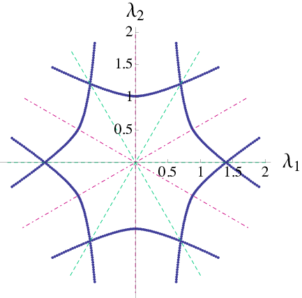
These are compared with the analytic ones. Figure 4 (a) is a plot of $(\mu_{1},\mu_{2})$ versus $(\lambda_{1},\lambda_{2})$ in the fundamental domain. The red and blue surfaces represent $\mu_{a}(\lambda_{i})$ $(a=1,2)$ in (207), respectively, whereas the red and blue points represent the numerical data $\lambda_{i}(\mu_{a})$ for given $\mu_{a}(=\bar{\mu}_{a})$ . Each horizontal sequence from the bottom to the top corresponds to $(\mu_{2})^{2/5}=1/2,1,3/2,2$ , with $\mu_{1}$ varied, while each vertical sequence from the left to the right corresponds to $(\mu_{1})^{2/5}=1/2,1,3/2,2$ , with $\mu_{2}$ varied. In Figure 4 (b), the diamonds ( $\diamond$ ) represent the projections of the points in (a) to the $(\lambda_{1},\lambda_{2})$ -plane. The horizontal solid lines are the contours of $\bigl(\mu_{2}(\lambda_{i})\bigr)^{2/5}=1/2,1,3/2,2$ from (207), while the vertical solid lines are the contours of $\bigl(\mu_{1}(\lambda_{i})\bigr)^{2/5}=1/2,1,3/2,2$ . We find good agreement between the analytic results and the numerical ones.

5.3 Inverse relation

The analytic mass-coupling relation (207) expresses the mass parameters $\mu_{a}$ as functions of the couplings $\lambda_{i}$ , whereas what one obtains numerically from the TBA equations is $\lambda_{i}$ as functions of $\mu_{a}$ , i.e., the inverse relation of (207). On dimensional grounds, a useful parametrization in the fundamental domain is

\displaystyle(\lambda_{1},\lambda_{2})=\mu_{1}^{2/5}\rho_{1}(\xi)\cdot w_{1}+\mu_{2}^{2/5}\rho_{2}(\xi)\cdot w_{2}\,,

(228)

(and similarly for $\bar{\lambda}_{i}(\bar{\mu}_{a})$ ), where $\rho_{a}\geq 0$ , $w_{i}$ are the fundamental weighs of $su(3)$ ; $w_{1}=(\sqrt{3},1)/\sqrt{6}$ , $w_{2}=(0,2)/\sqrt{6}$ ; and

\xi=\frac{\mu_{1}}{\mu_{2}}\ .\qquad

(229)

This parametrization generalizes, up to the power of $\mu_{a}$ , a classical one in [24]. (207) implies that $\xi$ is a function of $\eta=\lambda_{1}/\lambda_{2}$ . In Appendix H, we show that $\xi(\eta)$ is a monotonically increasing function in the fundamental domain, and its inverse $\eta(\xi)$ is well-defined. From the symmetry of the analytic relation under the chiral Dynkin transformation, $\mu_{1}\leftrightarrow\mu_{2}$ with $\bar{\mu}_{a}$ fixed, which is shown in Appendix G, it follows that

\rho_{2}(1/\xi)=\rho_{1}(\xi).

(230)

The inverse mass-coupling relations thus can be expressed in terms of a single function of one variable. Substituting (228) into (38), one also finds $(p_{2},p_{3})\to(p_{2},-p_{3})$ under the chiral Dynkin transformation, proving the relations (221) and (222) on the pCFT side. If $\rho_{a}$ were unity, (228) would give $\mu_{1}\sim\lambda_{1}^{5/2}$ , $\mu_{2}\sim(\sqrt{3}\lambda_{2}-\lambda_{1})^{5/2}$ . The relations (207) are generalizing these. From (228) and (207), one finds that $\rho_{a}$ take a simple form $x_{a}^{-1/2}F[x_{a}]$ with $x_{a}(\lambda_{j})$ being simple functions of $\lambda_{j}$ .

The differential equations for $\lambda_{i}$ or $\rho_{a}$ are derived by inverting the Jacobian matrix $\partial\mu_{a}/\partial\lambda_{i}$ , giving $\partial\lambda_{i}/\partial\mu_{a}$ . It is, however, difficult to solve them generally. Instead, let us first consider the asymptotic forms for $\mu_{1}\approx 0$ and $\mu_{2}\approx 0$ , corresponding to $\lambda_{1}\approx 0$ and $\sqrt{3}\lambda_{2}\approx\lambda_{1}$ , respectively. From (207) it follows that $F(1)\xi\approx(2\eta/\sqrt{3})^{2}$ , and hence

\rho_{1}(\xi)\approx c_{1}\xi^{1/10}+{\cal O}(\xi^{3/5})\,,\qquad\rho_{2}(\xi)\approx c_{2}(1-c_{3}\xi^{1/2})+o(\xi)\,,

(231)

for $\xi\ll 1$ . Here, the constants $c_{a}$ are

	$\displaystyle c_{1}=2^{3/10}B^{-2/5}\bigl[F(1)\bigr]^{1/10}\,,\qquad c_{2}=c_{1}\cdot\bigl[F(1)\bigr]^{-1/2}\,,$
	$\displaystyle c_{3}=\frac{2}{5}\bigl[F(1)\bigr]^{-1/2}\left(\frac{1}{2}F(1)-F^{\prime}(1)\right)\,.$		(232)

Similarly, one has $F(1)\xi^{-1}\approx\bigl((\sqrt{3}-\eta)/2\eta\bigr)^{2}$ and

\rho_{1}(\xi)\approx c_{2}(1-c_{3}\xi^{-1/2})+o(\xi^{-1})\,,\qquad\rho_{2}(\xi)\approx c_{1}\xi^{-1/10}+{\cal O}(\xi^{-3/5})\,,

(233)

for $\xi\gg 1$ .³³ 3 $F(x)$ has a branch point at $x=1$ , but $F^{\prime}(x)$ exists for $x\leq 1$ and Taylor’s theorem with Peano’s form of the remainder can be applied. The asymptotic behaviors are well approximated by functions of the form $\xi^{\pm 1/10}\sum c_{k}\xi^{\pm k/2}$ or $\sum c_{k}\xi^{\pm k/2}$ . From these, the special values of $\rho_{a}$ are read off,

$\displaystyle\rho_{1}(0)$	$\displaystyle=$	$\displaystyle\rho_{2}(\infty)=0\,,$
$\displaystyle\rho_{1}(\infty)$	$\displaystyle=$	$\displaystyle\rho_{2}(0)=c_{2}\approx 0.62317\,,$	(234)
$\displaystyle\rho_{1}(1)$	$\displaystyle=$	$\displaystyle\rho_{2}(1)=2^{1/10}\bigl[BF(1/2)\bigr]^{-2/5}\approx 0.49291\,.$

For reference, we have added the values at $\xi=1$ , corresponding to $\lambda_{2}=\sqrt{3}\lambda_{1}$ .

Generally, one can invert the relations (207) numerically. It is confirmed that the relation (230) indeed holds. Figure 5 is a plot of $\rho_{a}(\xi)$ obtained in this way. The blue points in the increasing sequence represent $\rho_{1}(\xi)$ , whereas the red points in the decreasing sequence represent $\rho_{2}(\xi)$ . The dashed lines indicate the special values in (234).

5.4 Comment on earlier work

Finally, we comment on an earlier work [33], where the mass-coupling relation of the $su(3)_{2}/u(1)^{2}$ HSG model was studied in order to evaluate the strong-coupling amplitudes of ${\cal N}=4$ SYM. Assuming that $\lambda_{i}$ are polynomials of $\mu_{a}^{2/5}$ , the couplings were parametrized as $\lambda_{i}=\sum_{a}\mu_{a}^{2/5}\hat{\lambda}_{ai}$ . The constants $\hat{\lambda}_{ai}$ were determined by matching the perturbative expression of $F_{2}$ in (39) and those in the perturbed minimal models corresponding to the single-mass and equal-mass cases in Section 3.2. The results were used for analytic expansions of the ground state energy and the Y-functions around the UV limit. It was observed that they appeared to be consistent with numerical data from the TBA equations within the numerical precision.

For the amplitudes, only the result of $F_{2}$ was used. The chiral factor $p_{2}$ of $F_{2}$ in (39) reads there

p_{2}^{HISS}=\frac{2}{3}\mu_{2}^{4/5}[r_{1}(1+\xi^{4/5})+r_{2}\xi^{2/5}]\,,

(235)

where

r_{1}=\rho_{2}^{2}(0)\,,\qquad r_{2}=3\rho^{2}_{2}(1)-2r_{1}\,.

(236)

With these constants, $p_{2}^{HISS}$ indeed matches the expression from (228),

p_{2}=\frac{2}{3}\mu_{2}^{4/5}[\rho_{2}^{2}+\rho_{1}\rho_{2}\xi^{2/5}+\rho_{1}^{2}\xi^{4/5}]\,,

(237)

at $\xi=0,1$ . Figure 6 is a plot of the relative deviation of the two expressions,

\delta_{p2}=\frac{p_{2}^{HISS}}{p_{2}}-1\,.

(238)

For simplicity, $\delta_{p2}$ is shown as a function of $\eta$ in the range $0\leq\eta=\lambda_{1}/\lambda_{2}\leq 1/\sqrt{3}$ , corresponding to $0\leq\xi\leq 1$ . The case with $\xi>1$ is covered by the Dynkin symmetry. One finds that the deviation is less than 1 per cent. It is still an open problem why a simple assumption in [33] works so well effectively. Other part of the analyses in [33] does not depend on the exact form of $F_{2}$ and hence need not be corrected. Similar remarks may apply to the analyses in [35] for the $su(3)_{4}/u(1)^{2}$ HSG model.

6 Vacuum expectation values from the mass-coupling relation

Given the mass-coupling relation, one can obtain the vacuum expectation values of the perturbing operators, which are the derivatives of the partition function with respect to the couplings. Indeed, in the course of the derivation of the analytic mass-coupling relation, a number of formulas have been found from the UV as well as the IR side: (99), (101), (108), (112) and (163).

To be concrete, $\langle\Phi_{ij}\rangle$ are for example given in terms of the couplings $\lambda_{i},\bar{\lambda}_{j}$ by (163), while those in terms of $\mu_{a},\bar{\mu}_{b}$ are obtained through the inverse relation (228). On the other hand, $\langle\Theta\rangle$ is simply given by the mass parameters as in (99), which is expressed by $\lambda_{i},\bar{\lambda}_{j}$ through the mass-coupling relation, e.g., (207) in the fundamental domain. In Figure 7 (a) and (b), we show plots of the vacuum expectation values as functions of the couplings, for examples of $\langle\Theta\rangle$ and $\langle\Phi_{11}\rangle$ . For simplicity, we have set $\lambda_{j}=\bar{\lambda}_{j}$ .

7 Conclusions

In this paper, we studied the mass-coupling relation of multi-scale quantum integrable models, focusing on the $su(3)_{2}/u(1)^{2}$ HSG model as their simplest example. Our basic strategy is to compare the conservation laws and the Ward identities of the integrable model both from the UV and IR points of view, which provides a novel method to analyze integrable models.

For this purpose, we first identified the relevant conserved currents on the UV side, and the dimension 3/5 operators on the IR side, which are the counterpart of the UV perturbing operators and characterized by their form factors. The representation of the coset in terms of the projected product of the minimal models provided an efficient calculational basis. It is notable that the products of minimal models allow multi-parameter integrable perturbations. Using the formulas for the response of the masses and S-matrix under the variation of the couplings, the perturbing operators $\Psi_{i}$ were expressed by the IR operators. This enabled us to express the conserved currents in terms of the IR operators. Comparing the conservation laws on the UV and the IR sides, the perturbing operators $\Phi_{ij}$ were also expressed by the IR operators. From the generalized $\Theta$ sum rule and the free energy Ward identity, the factorization of the mass-coupling relation (169) was shown.

The Ward identity for $\Phi_{ij}$ gave a differential equation of their one-point function. Together with the IR expression of $\Phi_{ij}$ , it was translated into a differential equation for the mass-coupling relation, which led to our main result (207). In the course of the derivation, we also obtained the vacuum expectation values of the perturbing operators. The resultant mass-coupling relation reproduced the known exact results in the single-mass cases, and agreed with the data obtained by solving the TBA equations numerically. Via the gauge-string duality, the relation provides the missing link to develop an analytic expansion of ten-particle strong-coupling scattering amplitudes of $\mathcal{N}=4$ SYM around the ${\mathbb{Z}}_{10}$ -symmetric (regular-polygonal) kinematic point.

Though we concentrated on the $su(3)_{2}/u(1)^{2}$ HSG model, our discussion in this paper is conceptually more general and can be applied to other multi-scale integrable models. Once a set of relevant form factors are given, the analysis of the mass-coupling relation would be straightforward. Our derivation also implies that one can obtain the differential equation for the one-point functions of the perturbing operators only through the UV conserved currents. Recalling the importance of differential equations in determining the correlations functions at the critical point, it would be an interesting future problem how powerful this Ward identity/differential equation is in determining the non-perturbative off-critical one-point functions.

Acknowledgements.

We would like to thank J. Luis Miramontes for useful conversations and László Fehér for a discussion on the Weyl reflection group. This work was supported by Japan-Hungary Research Cooperative Program. Z. B., J. B. and G. Zs. T. were supported by a Lendület Grant and by OTKA K116505, whereas K. I. and Y. S. were supported by JSPS Grant-in-Aid for Scientific Research, 15K05043 and 24540248 from Japan Society for the Promotion of Science (JSPS).

Appendix A Conventions

In this appendix, we summarize our conventions.

A.1 Space-time coordinates

We use the Minkowski space coordinates

x\sim(x^{0},x^{1})=(t,x),\qquad\quad x^{\pm}=t\pm x,

(239)

and for any 2-vector $W^{\mu}$ we define

W^{\pm}=W^{0}\pm W^{1},\qquad\quad W_{\pm}=\frac{1}{2}W^{\mp}.

(240)

The scalar product is

V\cdot W=V^{+}W_{+}+V^{-}W_{-}=\frac{1}{2}(V^{+}W^{-}+V^{-}W^{+}),\qquad\quad x^{2}=x^{+}x^{-}.

(241)

The derivatives are given as

\partial_{0}=\frac{\partial}{\partial t},\qquad\partial_{1}=\frac{\partial}{\partial x},\qquad\partial_{\pm}=\frac{1}{2}(\partial_{0}\pm\partial_{1}).

(242)

The Minkowski metric and antisymmetric tensor components are

\eta_{00}=-\eta_{11}=\epsilon_{01}=-\epsilon_{10}=1,\qquad\quad\eta_{01}=\eta_{10}=\epsilon_{00}=\epsilon_{11}=0,

(243)

and in light-cone coordinates

\eta^{++}=\eta^{--}=\epsilon^{++}=\epsilon^{--}=0,\qquad\quad\eta^{+-}=\eta^{-+}=\epsilon^{+-}=-\epsilon^{-+}=2.

(244)

In Euclidean space we use the coordinates $(x^{1},x^{2})$ , where $x^{2}=-\mathrm{i}x_{0}$ and the complex coordinates $z$ , $\bar{z}$ defined by

x^{+}=\mathrm{i}(x^{2}-\mathrm{i}x^{1})=\mathrm{i}z,\qquad\quad x^{-}=\mathrm{i}(x^{2}+\mathrm{i}x^{1})=\mathrm{i}\bar{z}.

(245)

So we have

-x^{2}=r^{2}=(x^{1})^{2}+(x^{2})^{2}=z\bar{z},\qquad\quad\partial=\frac{\partial}{\partial z}=\mathrm{i}\partial_{+},\qquad\quad\bar{\partial}=\frac{\partial}{\partial\bar{z}}=\mathrm{i}\partial_{-}.

(246)

A.2 Energy-momentum tensor

In the IR part of the paper we use the canonical energy-momentum tensor $T^{\mu\nu}$ , which is symmetric and conserved:

\partial_{-}T^{--}+\partial_{+}T^{+-}=0,\qquad\quad\partial_{+}T^{++}+\partial_{-}T^{-+}=0.

(247)

Its trace is denoted by

\Theta=T^{\mu}_{\,\,\mu}=T^{+-}.

(248)

The normalization of the canonical EM tensor is fixed by requiring that the total momentum operator

P_{\mu}=\int{\rm d}x\,T_{0\mu}(x,t)

(249)

acts on any local field $\Phi(x,t)$ according to

[P_{\mu},\Phi(x,t)]=-\mathrm{i}\partial_{\mu}\Phi(x,t).

(250)

In the UV part we use the CFT normalized Virasoro densities $L(z)$ , $\bar{L}(\bar{z})$ with the usual short distance expansion

L(z)L(w)\approx\frac{c}{2}\frac{1}{(z-w)^{4}}+\frac{2L(w)}{(z-w)^{2}}+\frac{\partial L(w)}{z-w},

(251)

where $c$ is the Virasoro central charge. For any chiral primary field $\Phi(z)$ with conformal weight $\Delta$ ,

L(z)\Phi(w)\approx\frac{\Delta\Phi(w)}{(z-w)^{2}}+\frac{\partial\Phi(w)}{z-w}.

(252)

There are analogous formulas for antichiral fields.

The identification of UV and IR fields is given by

L=\frac{\pi}{2}\,T^{--}=2\pi T_{++}.

(253)

Similarly

\bar{L}=\frac{\pi}{2}\,T^{++}=2\pi T_{--},\qquad\quad\tau=\frac{\pi}{2}\,T^{+-}=\frac{\pi}{2}\,\Theta,

(254)

where $\tau$ is the trace of the EM tensor in CFT normalization.

A.3 Equal time commutators in CFT

Equal time commutators are given in the CFT limit by the formulas

[P^{-},\Phi(z,\bar{z})]=-\pi\oint\frac{{\rm d}w}{2\pi\mathrm{i}}T^{--}(w)\Phi(z,\bar{z}),

(255)

[P^{+},\Phi(z,\bar{z})]=-\pi\oint\frac{{\rm d}\bar{w}}{2\pi\mathrm{i}}T^{++}(\bar{w})\Phi(z,\bar{z}).

(256)

Analogous formulas hold for any chiral conserved currents and charges.

A.4 Master formula

The master formula for the first order conformal perturbation is

\bar{\partial}L_{s}(z,\bar{z})=-\pi\oint\frac{{\rm d}w}{2\pi\mathrm{i}}{\cal L}_{\rm pert}(w,\bar{z})L_{s}(z)

(257)

for any chiral field $L_{s}(z)$ (in the CFT limit). Applying this to $L(z)$ we obtain, for a perturbation by a primary field with conformal weight $\Delta$ ,

	$\displaystyle\bar{\partial}L(z,\bar{z})$	$\displaystyle=$	$\displaystyle-\pi\oint\frac{{\rm d}w}{2\pi\mathrm{i}}{\cal L}_{\rm pert}(w,\bar{z})L(z)=-\pi\oint\frac{{\rm d}w}{2\pi\mathrm{i}}\left[\frac{\Delta{\cal L}_{\rm pert}(w,\bar{z})}{(z-w)^{2}}+\frac{\partial_{w}{\cal L}_{\rm pert}(w,\bar{z})}{z-w}\right]$		(258)
		$\displaystyle=$	$\displaystyle\pi(1-\Delta)\partial{\cal L}_{\rm pert}(z,\bar{z})=-\partial\tau.$		(258)

Thus we conclude that the CFT normalized trace is

\tau=-\pi(1-\Delta){\cal L}_{\rm pert},

(259)

whereas the trace of the canonical EM tensor is

\Theta=-2(1-\Delta){\cal L}_{\rm pert}.

(260)

Appendix B Characters

In this appendix, we summarize the relations among the $su(2)_{k}$ and the Virasoro characters, and the $su(3)_{2}$ string functions, which are used to confirm the relations among the coset theories and the minimal models in (3) and (4).

B.1 $su(2)_{k}$ and Virasoro characters

A unitary highest weight representation of $su(2)_{k}$ $(k\in{\mathbb{Z}}_{>0})$ has spin $l=0,1/2,\dots,k/2$ , and the central charge of the corresponding CFT is $c(su(2)_{k})=3k/(k+2)$ . We denote the character of the representation with spin $l$ by

{\rm ch}_{k,l}(\tau,\theta):=\mathrm{tr}\bigl(q^{L_{0}-c/24}\mathrm{e}^{\mathrm{i}\theta J_{0}^{3}}\bigr)\,,

(261)

where $q=\mathrm{e}^{2\pi\mathrm{i}\tau}$ , $c=c(su(2)_{k})$ , and $L_{0}$ and $J^{3}_{0}$ are the zero-modes of the Virasoro generators and one of the affine $su(2)$ currents.

The unitary minimal model ${\cal M}_{m,m+1}$ has the central charge $c({\cal M}_{m,m+1})=1-\frac{6}{m(m+1)}=:c_{m}$ . The spectrum consists of the primary fields $\phi^{(m)}_{r,s}$ with dimensions

h_{r,s}^{(m)}=\frac{[(m+1)r-ms]^{2}-1}{4m(m+1)}\,,

(262)

where $r=1,\dots,m-1$ ; $s=1,\dots,r$ . By the invariance under $r\to m-r$ and $s\to m+1-s$ , the range of $s$ may be extended to $s=1,\dots,m$ . The character of the representation with $(c_{m},h_{r,s}^{(m)})$ is given by

\chi^{(m)}_{h_{r,s}}(\tau):=\mathrm{tr}\bigl(q^{L_{0}-c_{m}/24}\bigr)=\eta^{-1}(\tau)\Bigl[\vartheta_{r(m+1)-sm,m(m+1)}(\tau)-\vartheta_{r(m+1)+sm,m(m+1)}(\tau)\Bigr]\,,

(263)

where

\eta(\tau)=q^{\frac{1}{24}}\prod_{n=1}^{\infty}(1-q^{n})\,,\qquad\vartheta_{m,k}(\tau)=\sum_{n\in{\mathbb{Z}}}q^{k\bigl(n+\frac{m}{2k}\bigr)^{2}}\,.

(264)

The superscript of $h^{(m)}_{r,s}$ has been omitted.

In terms of these characters, the coset representation of the minimal models $su(2)_{m-2}\times su(2)_{1}/su(2)_{m-1}={\cal M}_{m,m+1}$ implies [50]

{\rm ch}_{m-2,l}(\tau,\theta)\,{\rm ch}_{1,\epsilon}(\tau,\theta)=\sum_{s}{\rm ch}_{m-1,(s-1)/2}(\tau,\theta)\chi^{(m)}_{h_{r,s}}(\tau)\,,

(265)

where $\epsilon=0,1/2$ ; $r=2l+1$ ; $1\leq r\leq m-1$ ; $1\leq s\leq m$ ; and $r-s$ is even if $\epsilon=0$ and odd if $\epsilon=1/2$ . For $n=3$ the relation (4) reads

\frac{su(3)_{2}}{u(1)^{2}}\cong\frac{su(2)_{1}\times su(2)_{1}}{su(2)_{2}}\times\frac{su(2)_{2}\times su(2)_{1}}{su(2)_{3}}\,,

(266)

with the two factors $su(2)_{2}$ being identified. By this identification, the coset partition function consists of the terms of the form $\chi^{(3)}_{h}\chi^{(4)}_{h^{\prime}}$ where the two Virasoro characters share the common $su(2)_{2}$ in the decompositions, ${\rm ch}_{1,l}\,{\rm ch}_{1,\epsilon}=\sum_{s}{\rm ch}_{2,(s-1)/2}\chi^{(3)}_{h}$ and ${\rm ch}_{2,l}\,{\rm ch}_{1,\epsilon}=\sum_{s}{\rm ch}_{3,(s-1)/2}\chi^{(4)}_{h}$ . For example, one has $\chi^{(3)}_{h_{r,1}}$ $(r=1,2)$ with ${\rm ch}_{2,0}$ on the right side of the first decomposition, and $\chi^{(4)}_{h_{1,s}}$ $(s=1,\dots,4)$ with ${\rm ch}_{2,0}$ on the left side of the second decomposition. This gives $\phi_{r,1}^{(3)}\times\phi_{1,s}^{(4)}$ $(r=1,2;s=1,...,4)$ in the spectrum, which have the form of the projected products $\phi_{r,p}^{(m)}\phi_{p,s}^{(m+1)}$ [40]. Taking into account $\phi_{r,s}^{(m)}=\phi_{m-r,m+1-s}^{(m)}$ , and reducing the multiplicities by a factor two so that the identity appears only once, one finds the spectrum of $su(3)_{2}/u(1)^{2}$ in terms of the primaries of ${\cal M}_{3,4}$ and ${\cal M}_{4,5}$ as in (5).

B.2 $su(3)_{2}$ string functions and Virasoro characters in ${\cal M}_{3,4},{\cal M}_{4,5}$

Chiral fields in the $g_{k}/u(1)^{r_{g}}$ coset (generalized parafermion) theory are labeled by the highest weight $\Lambda$ and the weight $\lambda$ of $g_{k}$ as $\Phi^{\Lambda}_{\lambda}$ . The parafermionic character for $\Phi^{\Lambda}_{\lambda}$ is written as ${\rm ch}^{\Lambda}_{\lambda}(\tau):=\mathrm{tr}(q^{L_{0}-c/24})=\eta(\tau)^{r_{g}}c^{\Lambda}_{\lambda}(\tau)$ , where $c$ is the central charge, $r_{g}$ is the rank of $g$ and $c^{\Lambda}_{\lambda}$ is the string function.

For $su(3)_{2}$ , there are four independent string functions. Using the Dynkin labels, they read [51]

$\displaystyle c^{110}_{110}(\tau)$	$\displaystyle=$	$\displaystyle\eta(\tau)^{-4}\eta(2\tau)q^{1/20}\prod_{n\in{\mathbb{Z}}_{>0},n\neq\pm 1({\rm mod\,5})}(1-q^{2n})\,,$
$\displaystyle c^{200}_{011}(\tau)$	$\displaystyle=$	$\displaystyle\eta(\tau)^{-4}\eta(2\tau)q^{9/20}\prod_{n\in{\mathbb{Z}}_{>0},n\neq\pm 2({\rm mod\,5})}(1-q^{2n})\,,$
$\displaystyle c^{200}_{200}(\tau)-c^{200}_{011}(\tau)$	$\displaystyle=$	$\displaystyle\eta(\tau)^{-4}\eta(\tau/2)q^{1/80}\prod_{n\in{\mathbb{Z}}_{>0},n\neq\pm 1({\rm mod\,5})}(1-q^{n/2})\,,$	(267)
$\displaystyle c^{110}_{110}(\tau)-c^{110}_{002}(\tau)$	$\displaystyle=$	$\displaystyle\eta(\tau)^{-4}\eta(\tau/2)q^{9/80}\prod_{n\in{\mathbb{Z}}_{>0},n\neq\pm 2({\rm mod\,5})}(1-q^{n/2})\,.$

These are related to the products of the Virasoro characters in ${\cal M}_{3,4}\times{\cal M}_{4,5}$ as [52]

$\displaystyle\eta(\tau)^{2}c^{110}_{110}(\tau)$	$\displaystyle=$	$\displaystyle\chi_{\frac{1}{16}\frac{3}{80}}(\tau)=q^{-\frac{c}{24}+\frac{1}{10}}+\cdots\,,$
$\displaystyle\eta(\tau)^{2}c^{200}_{011}(\tau)$	$\displaystyle=$	$\displaystyle\chi_{\frac{1}{16}\frac{7}{16}}(\tau)=q^{-\frac{c}{24}+\frac{1}{2}}+\cdots\,,$
$\displaystyle\eta(\tau)^{2}c^{200}_{200}(\tau)$	$\displaystyle=$	$\displaystyle\chi_{00}(\tau)+\chi_{\frac{1}{2}\frac{3}{2}}(\tau)=q^{-\frac{c}{24}+0}+\cdots\,,$	(268)
$\displaystyle\eta(\tau)^{2}c^{110}_{002}(\tau)$	$\displaystyle=$	$\displaystyle\chi_{0\frac{3}{5}}(\tau)+\chi_{\frac{1}{2}\frac{1}{10}}(\tau)=2q^{-\frac{c}{24}+\frac{3}{5}}+\cdots\,,$

where $c=c_{3}+c_{4}=6/5$ and

\chi_{hh^{\prime}}(\tau):=\chi^{(3)}_{h}(\tau)\times\chi^{(4)}_{h^{\prime}}(\tau)\,.

(269)

In the main text, we have denoted $\chi_{h}^{(m)}$ $(m=3,4)$ by $\chi_{h}^{(i)}$ $(i=1,2)$ . Furthermore, with (263) one can check that

\chi_{\frac{1}{16}\frac{3}{80}}(\tau)=\chi_{0\frac{1}{10}}(\tau)+\chi_{\frac{1}{2}\frac{3}{5}}(\tau)\,,\qquad\chi_{\frac{1}{16}\frac{7}{16}}(\tau)=\chi_{\frac{1}{2}0}(\tau)+\chi_{0\frac{3}{2}}(\tau)\,.

(270)

Since the modular invariant for $su(3)_{2}$ is unique and diagonal [53], so is the modular invariant for $su(3)_{2}/u(1)^{2}$ :

	$\displaystyle Z\bigl(su(3)_{2}/u(1)^{2}\bigr)=\sum\bigl\|{\rm ch}^{\Lambda}_{\lambda}(\tau)\bigr\|^{2}$				(271)
			$\displaystyle\hskip-142.26378pt=\bigl\|\eta(\tau)\bigr\|^{4}\Bigl(\bigl\|c^{200}_{200}(\tau)\bigr\|^{2}+3\bigl\|c^{200}_{011}(\tau)\bigr\|^{2}+3\bigl\|c^{110}_{110}(\tau)\bigr\|^{2}+\bigl\|c^{110}_{002}(\tau)\bigr\|^{2}\Bigr)\,.$		(271)

From the relations among the string functions and the Virasoro characters given above, one finds that this modular invariant agrees with the one in (17). Given the multiplicities which are read off from the rightmost expressions in (268), one confirms the chiral field content: 1 identity, 3 fields with $h=1/2$ , 3 fields with $h=1/10$ and 2 fields with $h=3/5$ .

Appendix C Conserved charges from the counting argument

In this appendix we analyze conserved charges in the product picture in Section 2.2.

Spin 1 charges

Let us see how the counting argument works for the spin $s=2$ currents. We focus on the left chiral dependence as the right chiral part behaves as a spectator. We have 3 candidates to remain conserved after the perturbation, which correspond to the vectors⁴⁴ 4 Using the state-operator correspondence we often represent field operators by their corresponding vectors.:

|L_{-2}^{(1)}\rangle=\frac{1}{2}|\psi_{-\frac{3}{2}}\psi_{-\frac{1}{2}}\rangle\,,\qquad|L_{-2}^{(2)}\rangle\,,\qquad|L_{-2}^{(3)}\rangle=|\psi_{-\frac{1}{2}}G_{-\frac{3}{2}}\rangle\,.

(272)

These are the holomorphic stress tensor components in each theory $L^{(i)}(z)$ and the product $L^{(3)}(z)=\psi(z)G(z)$ . Clearly none is a total derivative. After the perturbation the level 1 subspace contains 3 vectors: $\psi_{-\frac{3}{2}}|{\scriptstyle\frac{1}{10}}\rangle$ , $L_{-1}G_{-\frac{1}{2}}|{\scriptstyle\frac{1}{10}}\rangle$ and $L_{-1}\psi_{-\frac{1}{2}}|{\scriptstyle\frac{1}{10}}\rangle$ , out of which only 1 is not a total derivative. The two total derivatives are the descendants of $\psi_{-\frac{1}{2}}|{\scriptstyle\frac{1}{10}}\rangle\sim|\Phi_{1j}\rangle$ and $G_{-\frac{1}{2}}|{\scriptstyle\frac{1}{10}}\rangle\sim|\Phi_{2j}\rangle$ as we are focusing only on the left chiral dependence. Comparing the dimensions we can conclude that two appropriate linear combinations of the $L^{(i)}$ have to be conserved. Clearly one of them corresponds to the energy $L(z)=L^{(1)}(z)+L^{(2)}(z)$ . The existence of the other conserved charge is consistent with the finding from the IR side (see Section 4) and can be obtained from short distance OPEs.

We calculate the relevant terms one by one:

L_{0}^{(1)}|\Phi_{1j}\rangle=\frac{1}{2}|\Phi_{1j}\rangle\,,\qquad L_{-1}^{(1)}|\Phi_{1j}\rangle=L_{-1}|\Phi_{1j}\rangle-\psi_{-\frac{1}{2}}\bar{\psi}_{-\frac{1}{2}}^{(j)}L_{-1}|\Phi\rangle\,,

(273)

\qquad L_{n}^{(1)}|\Phi_{2j}\rangle=0\quad(n=0,-1)\,.

(274)

The action of $L^{(2)}$ is

L_{0}^{(2)}|\Phi_{1j}\rangle=\frac{1}{10}|\Phi_{1j}\rangle\,,\quad L_{0}^{(2)}|\Phi_{2j}\rangle=\frac{3}{5}|\Phi_{2j}\rangle\,,\quad L_{-1}^{(2)}|\Phi_{ij}\rangle=\psi_{-\frac{1}{2}}^{(i)}\bar{\psi}_{-\frac{1}{2}}^{(j)}L_{-1}|\Phi\rangle\,.

(275)

Finally the action of $L_{0}^{(3)}=\dots\psi_{-\frac{1}{2}}G_{\frac{1}{2}}+\psi_{\frac{1}{2}}G_{-\frac{1}{2}}+\dots$ and $L_{-1}^{(3)}=\dots\psi_{-\frac{3}{2}}G_{\frac{1}{2}}+\psi_{-\frac{1}{2}}G_{-\frac{1}{2}}+\psi_{\frac{1}{2}}G_{-\frac{3}{2}}+\dots$ turns out to be

L_{0}^{(3)}|\Phi_{1j}\rangle=\frac{1}{\sqrt{5}}|\Phi_{2j}\rangle\,,\qquad L_{-1}^{(3)}|\Phi_{1j}\rangle=\frac{\sqrt{5}}{3}L_{-1}|\Phi_{2j}\rangle\,,

(276)

L_{0}^{(3)}|\Phi_{2j}\rangle=\frac{1}{\sqrt{5}}|\Phi_{1j}\rangle\,,\qquad L_{-1}^{(3)}|\Phi_{2j}\rangle=\frac{1}{\sqrt{5}}L_{-1}|\Phi_{1j}\rangle+\frac{4}{\sqrt{5}}\psi_{-\frac{1}{2}}^{(1)}\bar{\psi}_{-\frac{1}{2}}^{(j)}L_{-1}|\Phi\rangle\,,

(277)

where we used the super null vector $G_{-\frac{3}{2}}|\Phi\rangle=\frac{5}{3}G_{-\frac{1}{2}}L_{-1}^{(2)}|\Phi\rangle$ of the superconformal algebra. These formulas are used to calculate explicitly the second spin $1$ charge in Subsection 2.2.3.

Spin $2$ charges

In order to prove the factorization of the scattering matrix we need at least one higher spin charge. In [20] the authors used the coset chiral algebra and showed the existence of spin 2 conserved charges. As we are working with a smaller chiral algebra the counting argument does not guarantee any conserved charge at this level. Indeed, the possible candidates at the third level are

|\psi_{-\frac{5}{2}}\psi_{-\frac{1}{2}}\rangle\,,\quad|L_{-3}^{(2)}\rangle\,,\quad|G_{-\frac{5}{2}}\psi_{-\frac{1}{2}}\rangle\,,\quad|G_{-\frac{3}{2}}\psi_{-\frac{3}{2}}\rangle\,,

(278)

out of which only one is not a total derivative. On the other hand after the perturbation the level $2$ descendant space is

L_{-2}^{(2)}G_{-\frac{1}{2}}|{\scriptstyle\frac{1}{10}}\rangle\,,\quad(L_{-1}^{(2)})^{2}G_{-\frac{1}{2}}|{\scriptstyle\frac{1}{10}}\rangle\,,\quad(L_{-1}^{(2)})^{2}\psi_{-\frac{1}{2}}|{\scriptstyle\frac{1}{10}}\rangle\,,\quad G_{-\frac{1}{2}}\psi_{-\frac{3}{2}}\psi_{-\frac{1}{2}}|{\scriptstyle\frac{1}{10}}\rangle\,,

(279)

L_{-1}^{(2)}\psi_{-\frac{3}{2}}|{\scriptstyle\frac{1}{10}}\rangle\ ,\qquad\psi_{-\frac{5}{2}}|{\scriptstyle\frac{1}{10}}\rangle\,,

(280)

which contains three non-derivative operators and does not guarantee the existence of any conserved charge at this level. The reason why we could not find the spin 2 conserved charges is that we did not include in our chiral space (278) the contributions of the other two fermions of the representation spaces $2\chi_{\frac{1}{16}\frac{7}{16}}\bar{\chi}_{\frac{1}{16}\frac{7}{16}}$ .

Spin $3$ charges and integrability

Contrary to the spin 2 case our chiral algebra will be sufficient to find conserved charges at spin 3. In this case, we first analyze the operators of the chiral algebra $\mathcal{A}$ at level 4. We list the corresponding vectors:

|\psi_{-\frac{7}{2}}\psi_{-\frac{1}{2}}\rangle\,,\quad|\psi_{-\frac{5}{2}}\psi_{-\frac{3}{2}}\rangle\,,\quad|L_{-2}^{(2)}\psi_{-\frac{3}{2}}\psi_{-\frac{1}{2}}\rangle\,,\quad|L_{-2}^{(2)}L_{-2}^{(2)}\rangle\ ,\quad|L_{-4}^{(2)}\rangle\ ,

(281)

|L_{-2}^{(2)}G_{-\frac{3}{2}}\psi_{-\frac{1}{2}}\rangle\,,\quad|G_{-\frac{7}{2}}\psi_{-\frac{1}{2}}\rangle\,,\quad|G_{-\frac{5}{2}}\psi_{-\frac{3}{2}}\rangle\,,\quad|G_{-\frac{3}{2}}\psi_{-\frac{5}{2}}\rangle\,.

(282)

To see how many of them is not a total derivative we compare them to the states at the third level (278) and conclude that we have 5 non-derivative operators. As for the subspace after the perturbation, at the level 3 it contains the operators,

(L_{-1}^{(2)})^{3}\psi_{-\frac{1}{2}}|{\scriptstyle\frac{1}{10}}\rangle\,,\quad L_{-1}^{(2)}L_{-2}^{(2)}\psi_{-\frac{1}{2}}|{\scriptstyle\frac{1}{10}}\rangle\,,\quad L_{-1}^{(2)}L_{-2}^{(2)}G_{-\frac{1}{2}}|{\scriptstyle\frac{1}{10}}\rangle\,,\quad(L_{-1}^{(2)})^{3}G_{-\frac{1}{2}}|{\scriptstyle\frac{1}{10}}\rangle\,,

(283)

(L_{-1}^{(2)})^{2}\psi_{-\frac{3}{2}}|{\scriptstyle\frac{1}{10}}\rangle\,,\quad L_{-1}^{(2)}G_{-\frac{1}{2}}\psi_{-\frac{3}{2}}\psi_{-\frac{1}{2}}|{\scriptstyle\frac{1}{10}}\rangle\,,\quad L_{-1}^{(2)}\psi_{-\frac{5}{2}}|{\scriptstyle\frac{1}{10}}\rangle\,,\quad G_{-\frac{1}{2}}\psi_{-\frac{5}{2}}\psi_{-\frac{1}{2}}|{\scriptstyle\frac{1}{10}}\rangle\,,\quad\psi_{-\frac{7}{2}}|{\scriptstyle\frac{1}{10}}\rangle\,,

(284)

Again to see how many of them is not a total derivative we recall the states at one level higher (279), (280). Thus we have three non-derivative operators. This means that we can make two spin 3 conserved charges. This assures the quantum integrability of this model, as shown in [20]. Clearly the compatibility of the perturbations $\Phi_{i1}$ and $\Phi_{i2}$ again forces the coupling constant to factorize $\nu_{12}\nu_{21}=\nu_{11}\nu_{22}$ .

Appendix D Projected tensor product of minimal models

With extension to general cases in mind, in this appendix we discuss the identification between the $su(n)_{2}/u(1)^{n-1}$ coset CFT and the projected tensor product of the minimal models

\displaystyle{su(n)_{2}\over u(1)^{n-1}}=\mathbb{P}({\cal M}_{3,4}\times\cdots\times{\cal M}_{n+1,n+2}).

(285)

In the coset model $su(n)_{2}/u(1)^{n-1}$ , there are $n-1$ weight zero primary fields in the adjoint representation of $su(n)$ , whose conformal dimension is ${n\over n+2}$ , and which are used as the perturbation operators. In the projected tensor product the corresponding operators are represented as

\displaystyle\prod_{m=3}^{n+1}\phi^{(m)}_{k_{m},k_{m+1}},

(286)

where $k_{m}=1,3$ with $k_{m}\leq k_{m+1}$ , $k_{n+1}=3$ [54]. Here, the degenerate primary fields $\phi^{(m)}_{r,s}$ have conformal dimension $h_{r,s}^{(m)}$ as in (262). Since $k_{m}$ change only once, the products are of the form $1\times\cdots 1\times\phi_{1,3}^{(p)}\times\phi_{3,3}^{(p+1)}\times\cdots\phi_{3,3}^{(n+1)}$ ( $3\leq p\leq n+1$ ). Their conformal dimension is shown to be

\displaystyle\sum_{m=3}^{n+1}h^{(m)}_{k_{m},k_{m+1}}=\frac{p-1}{p+1}+\sum_{m=p+1}^{n+1}\frac{2}{m(m+1)}={n\over n+2}.

(287)

For example, in the $su(3)_{2}/u(1)^{2}$ model, one has the primary fields $\phi^{(3)}_{1,1}\phi^{(4)}_{1,3}$ and $\phi^{(3)}_{1,3}\phi^{(4)}_{3,3}$ in the projected product ${\mathbb{P}}({\cal M}_{3,4}\times{\cal M}_{4,5})$ as explained in Section 2.

In order to show the integrability of the HSG model, it is necessary to construct the conserved currents with integer spins. The quantum conserved currents with spin two and three have been constructed in [20]. In the projected product of minimal models, candidates of spin two conserved currents consist of the energy-momentum currents $L^{(m)}(z)$ for each minimal model ${\cal M}_{m,m+1}$ , and spin two operators $\phi^{(m)}_{1,3}\phi^{(m+1)}_{3,1}$ . They thus take the form

\displaystyle\Lambda=\sum_{l=3}^{n+1}\alpha_{l}L^{(l)}+\sum_{m=1}^{n}\beta_{m}\phi^{(m)}_{1,3}\phi^{(m+1)}_{3,1}

(288)

with some coefficients $\alpha_{l}$ and $\beta_{m}$ .

For the $su(3)_{2}/u(1)^{2}$ model, the primary field $\phi^{(3)}_{1,3}\phi^{(4)}_{3,1}$ is identified with the $L^{(i=3)}$ in the notation in Section 2 and Appendix C. Focusing on each chiral sector, the projected product can be reorganized into an ordinary tensor product in this special case [40], where the Virasoro characters $\chi_{h}^{(m)}$ $(m=3,4)$ are linearly combined into the chiral characters of the free fermion and the ${\cal N}=1$ super minimal model, respectively.

Appendix E Form factors

In this appendix we give all higher form factors corresponding to our tensor operators. We adapted the results of [47, 48] to our form factor conventions and field normalizations.

The $n$ -particle form factors of a local field operator $X$ are defined by the matrix elements

{\cal F}^{X}_{a_{1}\dots a_{n}}(\theta_{1},\dots,\theta_{n})=\langle 0|X(0)|\theta_{1},a_{1};\dots;\theta_{n},a_{n}\rangle,

(289)

where particle states are normalized according to

\langle\theta^{\prime},a^{\prime}|\theta,a\rangle=\delta_{a,a^{\prime}}\delta(\theta-\theta^{\prime}).

(290)

Below we give the “scalarized” form factors for our tensor operators for the case of $\ell=2s$ type-1 particles ( $s\geq 1$ ) and $m=2t$ type-2 particles ( $t\geq 1$ ). The total particle number is $n=\ell+m$ . The form factor polynomial can be written

q_{a_{1}\dots a_{n}}(x_{1},\dots,x_{n})=\widetilde{H}^{\ell,m}\,\widetilde{Q}^{\ell,m}_{a_{1}\dots a_{n}}(x_{1},\dots,x_{n}),

(291)

where the normalization constant $\widetilde{H}^{\ell,m}$ is given by

\widetilde{H}^{\ell,m}=\frac{(4\pi\mathrm{i})^{s(\ell-1)}}{(2\pi)^{s}}\,\widetilde{H}^{0,m}.

(292)

The lowest constants $\widetilde{H}^{0,m}$ still must be fixed from some further considerations. For example, from the normalization of the 2-particle form factors we can determine

\widetilde{H}^{0,2}=\mathrm{i}.

(293)

The polynomials are given as

\widetilde{Q}^{\ell,m}=(-1)^{(s+1)t}{\rm e}^{-t\sigma}\left(\Sigma^{(1)}\right)^{s-t}\left(\Sigma^{(2)}\right)^{t}\,{\cal D}^{s,t},

(294)

where

\Sigma^{(a)}=\prod_{a_{i}=a}x_{i}

(295)

and ${\cal D}^{s,t}$ is the determinant of an $(s+t-2)\times(s+t-2)$ matrix,

{\cal D}^{1,1}=1,\qquad\quad{\cal D}^{s,t}=\det({\cal M}^{s,t}),

(296)

whose matrix elements are symmetric polynomials,

\left({\cal M}^{s,t}\right)_{ij}=\left\{\begin{split}\sigma^{(1)}_{2j-2i+1}\qquad\qquad\quad&1\leq i<t,\\ (-1)^{j-i+t}\hat{\sigma}^{(2)}_{2j-2i+2t-1}\qquad&t\leq i\leq s+t-2.\end{split}\right.

(297)

The symmetric polynomials are defined by

\prod_{a_{i}=1}(z+x_{i})=\sum_{k=-\infty}^{\infty}z^{\ell-k}\sigma^{(1)}_{k},\qquad\quad\prod_{a_{i}=2}(z+x_{i}{\rm e}^{-\sigma})=\sum_{k=-\infty}^{\infty}z^{m-k}\hat{\sigma}^{(2)}_{k}.

(298)

Special cases are

\sigma^{(1)}_{1}=\hat{P}_{(1)}^{+},\qquad\hat{\sigma}^{(2)}_{1}={\rm e}^{-\sigma}\hat{P}_{(2)}^{+},\qquad\sigma^{(1)}_{\ell}=\Sigma^{(1)},\qquad\hat{\sigma}^{(2)}_{m}={\rm e}^{-m\sigma}\Sigma^{(2)}.

(299)

Appendix F Generalized $\Theta$ sum rule

In this appendix we describe a generalization of the well-known $\Theta$ sum rule [55], which is used in Section 4. Let us consider a conserved spin-2 current $Y^{\mu\nu}$ :

\partial_{\mu}Y^{\mu\nu}=0.

(300)

We do not assume that $Y^{\mu\nu}$ is symmetric and it need not be conserved in its second tensor index. Moreover, we do not assume that the theory is parity invariant.

Let us consider the Euclidean 2-point correlation function

C^{\mu\nu}(x)=\langle Y^{\mu\nu}(x)\Psi(0)\rangle_{c},

(301)

where $\Psi$ is some scalar field. From Euclidean (Lorentz) covariance it must be of the form

C^{\mu\nu}(x)=-x^{\mu}x^{\nu}\frac{F(r^{2})}{r^{4}}+\eta^{\mu\nu}\frac{A(r^{2})}{r^{2}}+\epsilon^{\mu\nu}\frac{B(r^{2})}{r^{2}},

(302)

and its components are

C^{+-}=\frac{F(r^{2})+2A(r^{2})+2B(r^{2})}{r^{2}}=\frac{G(r^{2})}{r^{2}},\qquad\quad C^{--}=\frac{\bar{z}^{2}F(r^{2})}{r^{4}}=\frac{F(r^{2})}{z^{2}}.

(303)

The conservation equation

\partial C^{+-}+\bar{\partial}C^{--}=0

(304)

is equivalent to

\frac{G}{r^{2}}=(F+G)^{\prime},

(305)

where ^′ here means derivative with respect to the argument $r^{2}$ . From here we have

\int{\rm d}^{2}x\langle Y^{+-}(x)\Psi(0)\rangle_{c}=\pi\int_{0}^{\infty}{\rm d}r^{2}\frac{G(r^{2})}{r^{2}}=\pi(F+G)|_{0}^{\infty}.

(306)

We assume that the theory is massive and therefore

F(\infty)=G(\infty)=0.

(307)

We also assume that the relevant conformal weights are $\Delta<1$ and so

G(0)=0.

(308)

We conclude that the integral of the scalar component is completely determined by the short distance asymptotics of the tensor component:

\int{\rm d}^{2}x\langle Y^{+-}(x)\Psi(0)\rangle_{c}=-\pi F(0),

(309)

where

\langle Y^{--}(x)\Psi(0)\rangle\approx\frac{F(0)}{z^{2}}.

(310)

If we apply these formulas to the EM tensor $T^{\mu\nu}$ and $\Psi$ is a scalar field with conformal weight $\Delta$ , we have

F(0)=\frac{2\Delta\langle\Psi\rangle}{\pi}

(311)

and

\int{\rm d}^{2}x\langle\Theta(x)\Psi(0)\rangle_{c}=-2\Delta\langle\Psi\rangle.

(312)

For the CFT normalized trace we have

\int{\rm d}^{2}x\langle\tau(x)\Psi(0)\rangle_{c}=-\pi\Delta\langle\Psi\rangle.

(313)

This is the $\Theta$ sum rule in its original form [55].

Appendix G Symmetries of the mass-coupling relation

In this appendix, we describe symmetries of the mass functions $\mu_{a}(\lambda_{1},\lambda_{2})$ , and their parametrization invariant under the symmetries.

G.1 $S_{3}$ Weyl symmetry

Our $\mu_{a}(\lambda_{1},\lambda_{2})$ functions ( $a=1,2$ ) satisfy the differential equation (185), as well as the scaling equation,

{\cal L}\mu_{a}=\frac{5}{2}\mu_{a}\,,\qquad{\cal L}=\lambda_{1}\partial_{1}+\lambda_{2}\partial_{2}\,.

(314)

The transformation rules for $\mu_{a}$ under the $S_{3}$ Weyl symmetry are

\hat{\mu}_{a}(\lambda_{1},\lambda_{2})=\mu_{a}(-\lambda_{1},\lambda_{2})\,,\qquad\check{\mu}_{a}(\lambda_{1},\lambda_{2})=\mu_{a}(\check{\lambda}_{1},\check{\lambda}_{2})\,,

(315)

where

\check{\lambda}_{1}=-\frac{1}{2}\lambda_{1}+\frac{\sqrt{3}}{2}\lambda_{2}\,,\qquad\check{\lambda}_{2}=-\frac{\sqrt{3}}{2}\lambda_{1}-\frac{1}{2}\lambda_{2}\,,

(316)

corresponding to a clockwise rotation by 120 degrees. Our differential equations are consistent with these discrete symmetries, since we can show that $\hat{\mu}_{a}$ and $\check{\mu}_{a}$ satisfy the same equations as $\mu_{a}$ . Using these one can extend the solution (207) outside the fundamental domain.

G.2 $\mu_{1}\Leftrightarrow\mu_{2}$ chiral Dynkin reflection

Next, let us consider the transformation,

\tilde{\lambda}_{1}=-\frac{1}{2}\lambda_{1}+\frac{\sqrt{3}}{2}\lambda_{2}\,,\qquad\tilde{\lambda}_{2}=\frac{\sqrt{3}}{2}\lambda_{1}+\frac{1}{2}\lambda_{2}\,,

(317)

which is the reflection with respect to the axis $\lambda_{2}=\sqrt{3}\lambda_{1}$ ( $\eta=1/\sqrt{3}$ ). Using the explicit solution in Subsection 4.9, we can show that

\mu_{1}(\tilde{\lambda}_{1},\tilde{\lambda}_{2})=\mu_{2}(\lambda_{1},\lambda_{2})\,.

(318)

From this symmetry it is sufficient to consider half of the fundamental domain, given by $0\leq\eta\leq 1/\sqrt{3}$ . The other half $1/\sqrt{3}\leq\eta\leq\sqrt{3}$ is mapped to the first half by this $\mu_{1}\Leftrightarrow\mu_{2}$ symmetry.

G.3 $S_{3}$ -invariant parametrization

To find the expression of $\mu_{a}(\lambda_{i})$ in the entire $(\lambda_{1},\lambda_{2})$ -plane, it is useful to adopt a $S_{3}$ -invariant parametrization,

2\mu_{a}=(p_{2})^{5/4}f_{a}(y)\,,

(319)

where $y=p_{3}^{2}/p_{2}^{3}$ and $p_{2}=\lambda_{1}^{2}+\lambda_{2}^{2}$ , $p_{3}=\lambda_{2}(\lambda_{2}^{2}-3\lambda_{1}^{2})$ as in (38). We note $0\leq y\leq 1$ for real $\lambda_{i}$ . The differential equation (185) then becomes

144y(1-y)f^{\prime\prime}_{a}(y)+72(1-y)f^{\prime}_{a}(y)-5f_{a}(y)=0\,,

(320)

whose general solutions are

f_{a}(y)=C_{a1}\cdot{}_{2}F_{1}\Bigl(-\frac{5}{12},-\frac{1}{12};\frac{1}{2};y\Bigr)+C_{a2}\cdot\sqrt{y}\,{}_{2}F_{1}\Bigl(\frac{1}{12},\frac{5}{12};\frac{3}{2};y\Bigr)\,.

(321)

The constants $C_{ak}$ $(a,k=1,2)$ are determined so as to match the mass-coupling relations in the equal- and single-mass cases discussed in Section 3.2, as done in [33]. The results are

C_{11}=C_{21}=\tilde{K}\,,\qquad C_{22}=-C_{12}=2\tilde{K}\frac{\Gamma(\frac{13}{12})\Gamma(\frac{17}{12})}{\Gamma(\frac{7}{12})\Gamma(\frac{11}{12})}\,,

(322)

where $\tilde{K}$ is given in (210). A useful identity in deriving these is

2=\frac{3^{1/4}}{\sqrt{2}\pi^{2}}\Gamma\Bigl(\frac{1}{4}\Bigr)^{2}\Gamma\Bigl(\frac{7}{12}\Bigr)\Gamma\Bigl(\frac{11}{12}\Bigr)\,.

(323)

In this expression, $f_{1}(y)\leq f_{2}(y)$ ( $0\leq y\leq 1$ ). Thus, smooth functions $\mu_{a}(\lambda_{i})$ are obtained by continuing $f_{1}$ and $f_{2}$ along the locus of $f_{1}(y)=f_{2}(y)$ , where $y=0$ , and $\lambda_{2}=\pm\sqrt{3}\lambda_{1}$ or $\lambda_{2}=0$ .

Appendix H $\xi$ - $\eta$ relation

In this appendix, we describe the relation between the ratios of the chiral masses $\mu_{a}$ and the couplings $\lambda_{i}$ . The result is used in Section 5.

For numerical studies we need the $\xi$ - $\eta$ relation, where

\xi=\frac{\mu_{1}}{\mu_{2}}=\frac{q_{1}(\eta)}{q_{2}(\eta)}\,,\qquad\eta=\frac{\lambda_{1}}{\lambda_{2}}\,,

(324)

and $q_{a}$ is defined in (182). The derivative of the $\xi(\eta)$ function is

\frac{d\xi}{d\eta}=\frac{W}{q_{2}^{2}}\,,

(325)

where $W$ is the Wronskian of the differential equation:

W=q^{\prime}_{1}q_{2}-q_{1}q^{\prime}_{2}\,.

(326)

It satisfies the differential equation,

\frac{W^{\prime}}{W}=\frac{12-2\eta^{2}}{\eta(\eta^{2}-3)}\,.

(327)

This can be used to determine $W$ explicitly. We find

W(\eta)=\frac{2\sqrt{3}B^{2}F(1)}{\eta^{4}}(3-\eta^{2})\,,

(328)

and

\frac{d\xi}{d\eta}=\frac{8\sqrt{3}F(1)\eta}{(\sqrt{3}-\eta)^{3}F^{2}\Bigl(\frac{\sqrt{3}-\eta}{\sqrt{3}+\eta}\Bigr)}\,,

(329)

with $F(z)$ defined in (188). From this expression we see that the derivative is positive. This means that $\xi(\eta)$ is monotonically increasing and its inverse is well-defined. In the fundamental domain, $0\leq\eta\leq\sqrt{3}$ , it is sufficient to determine this inverse function $\eta(\xi)$ for $0\leq\xi\leq 1$ ( $0\leq\eta\leq 1/\sqrt{3}$ ). For $\xi\geq 1$ ( $1/\sqrt{3}\leq\eta\leq\sqrt{3}$ ), it can be obtained using the formula

\eta(\xi)=\bar{\eta}(1/\xi)\,,

(330)

where

\bar{\eta}=\frac{\sqrt{3}-\eta}{1+\sqrt{3}\eta}\,.

(331)

References

(1) Giuseppe Mussardo, “Off critical statistical models: Factorized scattering theories and bootstrap program,” Phys. Rept. 218 (1992) 215.
(2) P. Dorey, “Exact S matrices”, In Conformal field theories and integrable models. Proceedings, Eotvos Graduate Course, Budapest, Hungary, August 13-18, 1996, (1996) 85. [hep-th/9810026]
(3) John L. Cardy and G. Mussardo, “S Matrix of the Yang-Lee Edge Singularity in Two-Dimensions,” Phys. Lett., B225 (1989) 275.
(4) A. B. Zamolodchikov, “Thermodynamic Bethe Ansatz in Relativistic Models. Scaling Three State Potts and Lee-yang Models,” Nucl. Phys. B 342 (1990) 695.
(5) A. B. Zamolodchikov, “Two point correlation function in scaling Lee-Yang model,” Nucl. Phys. B 348 (1991) 619.
(6) S. L. Lukyanov and A. B. Zamolodchikov, “Exact expectation values of local fields in quantum sine-Gordon model,” Nucl. Phys. B 493 (1997) 571 [hep-th/9611238].
(7) P. Hasenfratz, M. Maggiore and F. Niedermayer, “The Exact mass gap of the O(3) and O(4) nonlinear sigma models in d = 2,” Phys. Lett. B 245 (1990) 522.
(8) A. B. Zamolodchikov, “Mass scale in the sine-Gordon model and its reductions,” Int. J. Mod. Phys. A 10 (1995) 1125.
(9) P. Hasenfratz and F. Niedermayer, “The Exact mass gap of the O(N) sigma model for arbitrary $N>=3$ in d = 2,” Phys. Lett. B 245 (1990) 529.
(10) P. Forgacs, F. Niedermayer and P. Weisz, “The Exact mass gap of the Gross-Neveu model. 1. The Thermodynamic Bethe ansatz,” Nucl. Phys. B 367 (1991) 123.
(11) P. Forgacs, S. Naik and F. Niedermayer, “The Exact mass gap of the chiral Gross-Neveu model,” Phys. Lett. B 283 (1992) 282.
(12) J. Balog, S. Naik, F. Niedermayer and P. Weisz, “Exact mass gap of the chiral SU(n) x SU(n) model,” Phys. Rev. Lett. 69 (1992) 873.
(13) V. A. Fateev, E. Onofri and A. B. Zamolodchikov, “The Sausage model (integrable deformations of O(3) sigma model),” Nucl. Phys. B 406, 521 (1993).
(14) V. A. Fateev, “The Exact relations between the coupling constants and the masses of particles for the integrable perturbed conformal field theories,” Phys. Lett. B 324 (1994) 45.
(15) T. J. Hollowood, “The Exact mass gaps of the principal chiral models,” Phys. Lett. B 329 (1994) 450 [hep-th/9402084].
(16) J. M. Evans and T. J. Hollowood, “The Exact mass gap of the supersymmetric o(N) sigma model,” Phys. Lett. B 343 (1995) 189 [hep-th/9409141].
(17) J. M. Evans and T. J. Hollowood, “The Exact mass gap of the supersymmetric cp**(n-1) sigma model,” Phys. Lett. B 343 (1995) 198. [hep-th/9409142].
(18) V. A. Fateev and A. B. Zamolodchikov, “Integrable perturbations of Z(N) parafermion models and O(3) sigma model,” Phys. Lett. B 271 (1991) 91.
(19) C. R. Fernandez-Pousa, M. V. Gallas, T. J. Hollowood and J. L. Miramontes, “The symmetric space and homogeneous sine-Gordon theories,” Nucl. Phys. B 484 (1997) 609 [hep-th/9606032].
(20) C. R. Fernandez-Pousa, M. V. Gallas, T. J. Hollowood and J. L. Miramontes, “Solitonic integrable perturbations of parafermionic theories,” Nucl. Phys. B 499 (1997) 673 [hep-th/9701109].
(21) C. R. Fernandez-Pousa and J. L. Miramontes, “Semiclassical spectrum of the homogeneous sine-Gordon theories,” Nucl. Phys. B 518 (1998) 745 [hep-th/9706203].
(22) J. L. Miramontes and C. R. Fernandez-Pousa, “Integrable quantum field theories with unstable particles,” Phys. Lett. B 472 (2000) 392 [hep-th/9910218].
(23) O. A. Castro-Alvaredo, A. Fring, C. Korff and J. L. Miramontes, “Thermodynamic Bethe ansatz of the homogeneous Sine-Gordon models,” Nucl. Phys. B 575 (2000) 535 [hep-th/9912196].
(24) P. Dorey and J. L. Miramontes, “Mass scales and crossover phenomena in the homogeneous sine-Gordon models,” Nucl. Phys. B 697 (2004) 405 [hep-th/0405275].
(25) O. A. Castro-Alvaredo and A. Fring, “Renormalization group flow with unstable particles,” Phys. Rev. D 63 (2001) 021701 [hep-th/0008208].
(26) O. A. Castro-Alvaredo and A. Fring, “Decoupling the SU(n)(2) homogeneous Sine-Gordon model,” Phys. Rev. D 64 (2001) 085007 [hep-th/0010262].
(27) L. F. Alday and J. M. Maldacena, “Gluon scattering amplitudes at strong coupling,” JHEP 0706 (2007) 064 [arXiv:0705.0303 [hep-th]].
(28) L. F. Alday and J. Maldacena, “Null polygonal Wilson loops and minimal surfaces in Anti-de-Sitter space,” JHEP 0911 (2009) 082 [arXiv:0904.0663 [hep-th]].
(29) L. F. Alday, D. Gaiotto and J. Maldacena, “Thermodynamic Bubble Ansatz,” JHEP 1109 (2011) 032 [arXiv:0911.4708 [hep-th]].
(30) L. F. Alday, J. Maldacena, A. Sever and P. Vieira, “Y-system for Scattering Amplitudes,” J. Phys. A 43 (2010) 485401 [arXiv:1002.2459 [hep-th]].
(31) Y. Hatsuda, K. Ito, K. Sakai and Y. Satoh, “Thermodynamic Bethe Ansatz Equations for Minimal Surfaces in $AdS_{3}$ ,” JHEP 1004 (2010) 108 [arXiv:1002.2941 [hep-th]].
(32) Y. Hatsuda, K. Ito, K. Sakai and Y. Satoh, “Six-point gluon scattering amplitudes from $Z_{4}$ -symmetric integrable model,” JHEP 1009 (2010) 064 [arXiv:1005.4487 [hep-th]].
(33) Y. Hatsuda, K. Ito, K. Sakai and Y. Satoh, “g-functions and gluon scattering amplitudes at strong coupling,” JHEP 1104 (2011) 100 [arXiv:1102.2477 [hep-th]].
(34) Y. Hatsuda, K. Ito and Y. Satoh, “T-functions and multi-gluon scattering amplitudes,” JHEP 1202 (2012) 003 [arXiv:1109.5564 [hep-th]].
(35) Y. Hatsuda, K. Ito and Y. Satoh, “Null-polygonal minimal surfaces in $AdS_{4}$ from perturbed W minimal models,” JHEP 1302 (2013) 067 [arXiv:1211.6225 [hep-th]].
(36) Y. Hatsuda, K. Ito, Y. Satoh and J. Suzuki, “Quantum Wronskian approach to six-point gluon scattering amplitudes at strong coupling,” JHEP 1408 (2014) 162 [arXiv:1406.5904 [hep-th]].
(37) Z. Bajnok, J. Balog, K. Ito, Y. Satoh and G. Z. Tóth, “Exact mass-coupling relation for the homogeneous sine-Gordon model,” Phys. Rev. Lett. 116 (2016) 181601 [arXiv:1512.04673 [hep-th]].
(38) V. A. Fateev and A. B. Zamolodchikov, “Parafermionic Currents in the Two-Dimensional Conformal Quantum Field Theory and Selfdual Critical Points in Z(n) Invariant Statistical Systems,” Sov. Phys. JETP 62 (1985) 215 [Zh. Eksp. Teor. Fiz. 89 (1985) 380].
(39) D. Gepner and Z. -a. Qiu, “Modular Invariant Partition Functions for Parafermionic Field Theories,” Nucl. Phys. B 285 (1987) 423.
(40) C. Crnkovic, R. Paunov, G. M. Sotkov and M. Stanishkov, “Fusions of Conformal Models,” Nucl. Phys. B 336 (1990) 637.
(41) J. Bagger and D. Nemeschansky, “Coset Construction Of Chiral Algebras,” HUTP-88/A059.
(42) P. Bouwknegt and K. Schoutens, “W symmetry in conformal field theory,” Phys. Rept. 223 (1993) 183 [hep-th/9210010].
(43) E. Ardonne and K. Schoutens, “Wavefunctions for topological quantum registers,” Annals Phys. 322 (2007) 201 [cond-mat/0606217].
(44) A. B. Zamolodchikov, “Integrals of Motion in Scaling Three State Potts Model Field Theory,” Int. J. Mod. Phys. A 3 (1988) 743.
(45) A. B. Zamolodchikov, “Integrable field theory from conformal field theory,” Adv. Stud. Pure Math. 19 (1989) 641.
(46) Al. B. Zamolodchikov, “Thermodynamic Bethe ansatz for RSOS scattering theories,” Nucl. Phys. B 358 (1991) 497.
(47) O. A. Castro-Alvaredo, A. Fring and C. Korff, “Form-factors of the homogeneous Sine-Gordon models,” Phys. Lett. B 484 (2000) 167 [hep-th/0004089].
(48) O. A. Castro-Alvaredo and A. Fring, “Identifying the operator content, the homogeneous sine-Gordon models,” Nucl. Phys. B 604 (2001) 367 [hep-th/0008044].
(49) G. Delfino, G. Mussardo and P. Simonetti, “Nonintegrable quantum field theories as perturbations of certain integrable models,” Nucl. Phys. B 473 (1996) 469 [hep-th/9603011].
(50) P. Goddard, A. Kent and D. I. Olive, “Unitary Representations of the Virasoro and Supervirasoro Algebras,” Commun. Math. Phys. 103 (1986) 105.
(51) V. G. Kac and D. H. Peterson, “Infinite dimensional Lie algebras, theta functions and modular forms,” Adv. Math. 53 (1984) 125.
(52) M. Ninomiya and K. Yamagishi, “Nonlocal Su(3) Current Algebra,” Phys. Lett. B 183 (1987) 323.
(53) T. Gannon, “The Classification of affine SU(3) modular invariant partition functions,” Commun. Math. Phys. 161 (1994) 233 [hep-th/9212060].
(54) V. G. Kac and M. Wakimoto, “Modular and conformal invariance constraints in representation theory of affine algebras,” Adv. Math. 70 (1988) 156.
(55) G. Delfino, P. Simonetti and J. L. Cardy, “Asymptotic factorization of form-factors in two-dimensional quantum field theory,” Phys. Lett. B 387 (1996) 327 [hep-th/9607046].
(56) F. Constantinescu and R. Flume, “The convergence of strongly relevant perturbations of $D=2$ conformal field theories,” Phys. Lett. B 326 (1994) 101.

On the mass-coupling relation of multi-scale quantum integrable models

Abstract

1 Introduction

2 Homogeneous sine-Gordon model as a perturbed CFT

2.1 Coset representation

2.2 Minimal models product representation

2.2.1 The chiral algebra

The Ising part

The tricritical Ising part

2.2.2 The Hilbert space of the product model

2.2.3 Perturbation and conserved charges

2.3 Ground state energy from perturbed CFT

3 Homogeneous sine-Gordon model as a scattering theory

3.1 S-matrix and TBA

3.2 Special cases

Single-mass cases (𝐦𝟏=𝟎\mathbf{m_{1}=0} or 𝐦𝟐=𝟎\mathbf{m_{2}=0})

Equal-mass case (𝐦𝟏=𝐦𝟐\mathbf{m_{1}=m_{2}})

3.3 Form factors of the dimension 3/53/5 operators

3.4 Numerical check of the dimension

4 Analytical mass-coupling relation

4.1 Exact VEVs and relations from changing the couplings

4.2 Relations among the local operators

4.3 Relations from conserved spin 1 charges: factorization of mass ratios

4.4 Relations from conserved tensor currents

4.5 Relation between the UV and IR bases

4.6 Free energy Ward identity

4.7 Proof of complete factorization

4.8 Mass-coupling relation

4.9 Solution of the differential equation

5 Numerical mass-coupling relation

5.1 UV expansion coefficients of the ground state energy from TBA

5.2 Numerical mass-coupling relation

5.3 Inverse relation

5.4 Comment on earlier work

6 Vacuum expectation values from the mass-coupling relation

7 Conclusions

Acknowledgements.

Appendix A Conventions

A.1 Space-time coordinates

A.2 Energy-momentum tensor

A.3 Equal time commutators in CFT

A.4 Master formula

Appendix B Characters

B.1 s​u​(2)ksu(2)_{k} and Virasoro characters

B.2 s​u​(3)2su(3)_{2} string functions and Virasoro characters in ℳ3,4,ℳ4,5{\cal M}_{3,4},{\cal M}_{4,5}

Appendix C Conserved charges from the counting argument

Spin 1 charges

Spin 22 charges

Spin 33 charges and integrability

Appendix D Projected tensor product of minimal models

Appendix E Form factors

Appendix F Generalized Θ\Theta sum rule

Appendix G Symmetries of the mass-coupling relation

G.1 S3S_{3} Weyl symmetry

G.2 μ1⇔μ2\mu_{1}\Leftrightarrow\mu_{2} chiral Dynkin reflection

G.3 S3S_{3}-invariant parametrization

Appendix H ξ\xi-η\eta relation

References

Single-mass cases ( $\mathbf{m_{1}=0}$ or $\mathbf{m_{2}=0}$ )

Equal-mass case ( $\mathbf{m_{1}=m_{2}}$ )

3.3 Form factors of the dimension $3/5$ operators

B.1 $su(2)_{k}$ and Virasoro characters

B.2 $su(3)_{2}$ string functions and Virasoro characters in ${\cal M}_{3,4},{\cal M}_{4,5}$

Spin $2$ charges

Spin $3$ charges and integrability

Appendix F Generalized $\Theta$ sum rule

G.1 $S_{3}$ Weyl symmetry

G.2 $\mu_{1}\Leftrightarrow\mu_{2}$ chiral Dynkin reflection

G.3 $S_{3}$ -invariant parametrization

Appendix H $\xi$ - $\eta$ relation