Explicit symplectic algorithms based on generating functions for charged particle dynamics

The dynamics of a charged particle with the Lorentz force in the canonical coordinates $(\mathbf{x},\mathbf{p})$ is a canonical Hamiltonian system,

where $\mathbf{Z}=(\mathbf{x}^{T},\mathbf{p}^{T})^{T}$ is a 6-dimensional vector,

is the canonical symplectic matrix and

is the Hamiltonian function. For canonical Hamiltonian system

it is well known that symplectic algorithms conserve the symplectic structure exactly and globally bound the energy error by a small number [1, 2, 3, 4, 5, 6, 7, 8, 9, 10, 11, 12, 13, 14]. They have become the de facto standard for numerical integration of Hamiltonian systems with important applications in nonlinear dynamics, astrophysics, plasma physics, accelerator physics, and quantum physics. Recently, symplectic and geometric algorithms have been developed for non-canonical particle dynamics [15, 16, 17, 18, 19, 20, 21, 22, 23, 24, 25, 26, 27, 28] and the infinite dimensional particle-field systems [29, 30, 31, 32, 33, 34, 35, 36, 37, 38, 39, 40, 41, 42, 43] in plasma physics and accelerator physics. To improve the efficiency and accuracy of long-term simulations for systems with a large number, e.g., $10^{9}$, of degrees of freedom, explicit symplectic algorithms are desired. Strictly speaking, in order for implicit symplectic algorithms to be symplectic, the implicit iteration relations need to be solved exactly, which is impossible in general. The best one can expect is to solve the implicit iteration relations to machine precision at an extreme cost. This is the main reason to search for explicit symplectic method. Splitting method has been proven to be an effective tool in constructing explicit symplectic algorithms [44, 45, 46, 47, 48, 24, 22, 38, 39]. The basic procedure is to decompose original system into solvable subsystems possessing the same geometric structure, then compose the geometric sub-algorithms together to obtain the desired algorithms [44, 49, 13]. It is well known that for a Hamiltonian whose $\mathrm{\mathbf{p}}$-dependence and $\mathbf{q}$-dependence can be separated as sumands in a summation as follows

the splitting method can generate explicit symplectic algorithms of any orders [7, 5]. The familiar leapfrog algorithm is an example of this method. We will call the form in Eq. (4) sum-separable and refer to this well-known splitting method as sum-split method. It is generally believed that if a Hamiltonian is not sum-separable as in Eq. (4), general explicit symplectic algorithms do not exist [11, 44, 47, 50, 14, 51, 13]. For dynamics of charged particle, sum-split method loses efficacy and can not be applied directly to construct explicit symplectic algorithms, because the Hamiltonian Eq. (2) is not sum-separable. An explicit non-canonical symplectic algorithm has been developed by He et al. using sum-split method for charged particle dynamics in the non-canonical coordinates [25, 40, 37]. However, it requires numerical integration of the magnetic field along given paths, which can be non-trivial for certain complicated magnetic fields. In this paper, different from He’s splitting algorithm, we combine the familiar sum-split method with a generating function method to construct explicit symplectic algorithms for dynamics of charged particles, which do not require numerical integration of the magnetic field.

The generating function method has been well developed to construct symplectic methods for a Hamiltonian system Eq. (3) [4, 13, 14]. There are three types generating functions utilized to construct different types of symplectic algorithms. The symplectic Euler method and mid-point method are included in this family. Generally speaking, symplectic methods based on all three types of generating functions are usually implicit. However, for product-separable Hamiltonians in the form of

or

explicit symplectic algorithms with accuracy of order 2 and 3 can be constructed by applying the first type generating function and the second type generating function respectively. Here, product-separable means that the $\mathbf{q}$-dependency and $\mathbf{p}$-dependency can be separated as factors in a production. For dynamics of charged particle governed by Eq. (1), we sum-split the Hamiltonian Eq. (2) into five parts, two of which can be solved exactly. The other three parts are in the form of Eq. (5), and admit explicit symplectic algorithms based on the generating functions. Then combining the exact solution flows and explicit symplectic sub-algorithms in various manners, explicit symplectic algorithms of different orders can be constructed.

The paper is organized as follows. In Sec. II, symplectic algorithms based on generating functions are introduced, and for the Hamiltonian systems with the forms of Eqs. (5) and (6), explicit symplectic algorithms are given. In Sec. III, we construct explicit symplectic algorithms of order 2 and 3 for charged particle dynamics based on generating functions. Numerical experiments are provided, and the superiority of the explicit symplectic algorithms relative to non-symplectic Runge-Kutta methods and implicit symplectic methods is demonstrated in Sec. IV.

For a Hamiltonian system Eq. (3), we introduce symplectic methods based on the first and second type of generating functions. The symplectic methods based on generating functions of the first type can be written as

with the generating function

where

Utilizing the truncated series,

we obtain a symplectic method of order $r$ [4, 13, 14]. The symplectic methods based on generating functions of the second type can be constructed similarly. Both types are usually implicit for general Hamiltonian systems. However, for product-separable Hamiltonian with the form of Eq. (5) or Eq. (6), second and third order symplectic algorithms based on generating functions can be constructed explicitly. Let’s take Hamiltonian Eq. (5) as an example to demonstrate the explicit symplectic methods based on the generating functions. The corresponding second order generating function of type one is

Then the explicit symplectic method of order 2 based on the generating function is

For the product-separable Hamiltonian in the form of Eq. (6), explicit symplectic algorithms can be constructed similarly utilizing generating functions of the second type.

In this section, we will use the methods given in Sec. II to construct explicit symplectic algorithms for charged particle dynamics determined by Eq. (1). It was commonly believed that this system does not admit any explicit symplectic algorithm, because the Hamiltonian given by Eq. (2) is not sum-separable. Now, we show how to construct explicit symplectic algorithms for it using the generating-function method and the familiar sum-split method. We sum-split the Hamiltonian function into five parts as

where

The corresponding sub-systems generated by these sub-Hamiltonians are

For subsystems $S_{1}$ and $S_{2}$, exact solutions can be computed explicitly as

The sub-Hamiltonians of remaining three subsystems $S_{3}$, $S_{4}$ and $S_{5}$ are all product-separable as in Eq. (5). Let’s take the sub-system $S_{3}$ associated with the sub-Hamiltonian $H_{3}(\mathbf{p},\mathbf{x})=-\dfrac{q}{m}p_{1}\mathbf{A}_{1}(\mathbf{x})$ as an example to demonstrate our method. In terms of Cartesian components, the sub-system $S_{3}$ is

The symplectic method of order 2 based on generating function can be obtained,

where the truncated generating function of order 2 is

Thus, the second-order symplectic methods for $S_{3}$ is

which is an explicit method, but not symmetric. For sub-systems $S_{4},$ and $S_{5}$, second order explicit symplectic methods $\psi_{4}^{\Delta t}$ and $\psi_{5}^{\Delta t}$ are constructed similarly. Composing the exact solutions and the symplectic numerical flows of the five subsystems, we obtain the following explicit symplectic method for charged particle dynamics with the accuracy of order 1,

If the sub-numerical solution $\psi_{3}^{\Delta t}$, $\psi_{4}^{\Delta t}$, and $\psi_{5}^{\Delta t}$ were symmetric, the symplectic method obtained by symmetric composition

would be symmetric and of order 2. Because $\psi_{3}^{\Delta t}$, $\psi_{4}^{\Delta t}$, and $\psi_{5}^{\Delta t}$ are not symmetric, neither is $\Psi_{\Delta t}^{2}$. However, we can prove that $\Psi_{\Delta t}^{2}$ is of second order. The proof is given in the Appendix. Since all the sub-algorithms preserve the canonical symplectic structure, $\Psi_{\Delta t}^{1}$ and $\Psi_{\Delta t}^{2}$ preserve the canonical symplectic structure naturally. Of course, it is possible to increase the accuracy of the numerical methods by various compositions [44, 13]. For example, a third order algorithm can be obtained by the following composition method using $\Psi_{\Delta t}^{2}$,

where $a=\dfrac{1}{2-2^{1/3}}$ and $b=1-2a$. To numerically verify the orders of $\Psi_{\Delta t}^{2}$ and $\Psi_{\Delta t}^{3}$, we now apply $\Psi_{\Delta t}^{2}$, $\Psi_{\Delta t}^{3}$, the second order implicit mid-point method and a 4th-order implicit symplectic method to simulate the dynamics of charged particle in the magnetic field of a tokamak (see next section). Here, the 4th-order implicit symplectic method is generated by symmetric composition of the second order implicit mid-point method. The relative errors of Hamiltonian as functions of time step $\Delta t$ for these methods are plotted in Fig. 1, which verifies that $\Psi_{\Delta t}^{2}$ is indeed a second order method and $\Psi_{\Delta t}^{3}$ is a third order method.

To numerically test the explicit symplectic algorithms developed, we simulate the dynamics of a $3.5$MeV $\alpha-$particle, which is a product of D-T fusion, in the magnetic field of a tokamak. We will compare the second order explicit symplectic (ES2) method $\Psi_{\Delta t}^{2}$ developed with the second order implicit symplectic mid-point (IS2) method and the third order non-symplectic Runge-Kutta (RK3) method. Numerical results will demonstrate the superb properties of explicit symplectic methods in terms of accuracy, efficiency and preserving energy over long-term simulations.

The axisymmetric tokamak geometry is illustrated in Fig. 2. A model vector potential of the magnetic field is

where $R=\sqrt{x^{2}+y^{2}}$ is the major radius coordinate, $R_{0}$ is the major radius, $B_{0}$ is the magnetic field on axis, the constant $q$ is the safety factor, and $\zeta=arctan\left(\frac{x}{y}\right)$ is the toroidal coordinate of the torus. In this example, we take $R_{0}=3m$ and $B_{0}=1T$ with $q=2$.

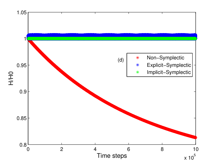
The initial position and velocity of the $\alpha-$particle are $\mathbf{x}_{0}=(3.15,0,0)m$ and $\mathbf{v}_{0}=(0.016,0.04,0)c$, where $c$ is the speed of light, and the simulation time-step is set to be $\text{$\Delta$}t=0.1\times 10^{-8}s$. Displayed in Fig. 3 is the comparison of transit orbits calculated by the non-symplectic third order Runge-Kutta (RK3) method, second order implicit symplectic mid-point (IS2) method and the explicit second symplectic (ES2) algorithm $\Psi_{\Delta t}^{2}$. It is expected that the orbit consists of a fast, small scale gyro-motion due to Lorentz force, and a slow, large scale transit motion induced by the inhomogeneity of the magnetic field. In Fig. 3, the small circles of a few centimeters are the fast gyro-motion, and the large circles about half meter in size in the $RZ-$ plane is the large scale transit dynamics. Figure. 3(a) shows that the orbit obtained by the non-symplectic RK3 method after $9.8\times 10^{5}$ time steps is not accurate any more, while the orbits calculated by the IS2 method in Fig. 3(b) and ES2 algorithm $\Psi_{\Delta t}^{2}$ in Fig. 3(c) are accurate for all time steps and form closed transit orbits. The long-term energy by non-symplectic method gradually decreases without bound due to numerical errors. On the contrary, for the symplectic integrators, the energy errors are bounded by a small number for all time. This fact is clearly demonstrated in Fig. 3(d), where normalized energy for the three algorithms are plotted.

To illustrate the efficiency of the explicit symplectic algorithms developed, the CPU time used by the three methods for calculating the charged particle dynamics is listed in Table. 1. The numerical calculation consists of $10^{6}$ time-steps, and is carried using on a Inter Core $i5-4200U$ CPU. It’s clear that the ES2 algorithm $\Psi_{\Delta t}^{2}$ is much more efficient than the IS2 algorithm.

In this paper, we have constructed explicit symplectic algorithms for dynamics of charged particle by combining the familiar sum-split method with a specially designed generating function method. The newly developed algorithms are expected to significantly extend the applicability of symplectic algorithms to physics problems which contain a large number of degrees of freedom and require accuracy, fidelity and efficiency of long-term dynamics, such as the classical particle-field system described by the Vlasov-Maxwell equations [52].

We will prove the explicit algorithm $\Psi_{\Delta t}^{2}$ given by Eq. (22) is a second order method for the Hamiltonian

To simplify the notation, we have taken $m=1$ and $q=1.$ There are three steps in the proof.

Step 1: To prove $\psi_{3}^{\Delta t/2}\circ\psi_{4}^{\Delta t/2}\circ\psi_{5}^{\Delta t}\circ\psi_{4}^{\Delta t/2}\circ\psi_{3}^{\Delta t/2}$ is a numerical method of order 2 for the sub-Hamiltonian system with Hamiltonian

Since $\psi_{2+i}^{\Delta t},\>i=1,2,3,$ is numerical method of order 2 for Hamiltonian system generated by $H_{2+i}=-\mathbf{p}_{i}\mathbf{A}_{i}(\mathbf{x})$, it can be rewritten as

where $\mathbf{e}_{i}$ is the unit vector in the $i$-th Cartesian direction. The composition method $\psi_{3}^{\Delta t/2}\circ\psi_{4}^{\Delta t/2}\circ\psi_{5}^{\Delta t}\circ\psi_{4}^{\Delta t/2}\circ\psi_{3}^{\Delta t/2}$ can be obtained using the iterations step by step as follows,

where $\mathbf{V}_{ij}=\mathbf{p}_{i}\dfrac{\partial\mathbf{A}_{i}}{\partial\mathbf{x}_{j}}\nabla\mathbf{A}_{j}-\mathbf{p}_{j}\mathbf{A}_{i}\nabla\dfrac{\partial\mathbf{A}_{j}}{\partial\mathbf{x}_{i}}$. This shows that the $\psi_{3}^{\Delta t/2}\circ\psi_{4}^{\Delta t/2}\circ\psi_{5}^{\Delta t}\circ\psi_{4}^{\Delta t/2}\circ\psi_{3}^{\Delta t/2}$ is of order 2.

Step 2: To prove $\varphi_{2}^{\Delta t/2}\circ\psi_{3}^{\Delta t/2}\circ\psi_{4}^{\Delta t/2}\circ\psi_{5}^{\Delta t}\circ\psi_{4}^{\Delta t/2}\circ\psi_{3}^{\Delta t/2}\circ\varphi_{2}^{\Delta t/2}$ is of order 2 for the sub-Hamiltonian system with Hamiltonian

As proved in Step 1, the iteration $\psi_{3}^{\Delta t/2}\circ\psi_{4}^{\Delta t/2}\circ\psi_{5}^{\Delta t}\circ\psi_{4}^{\Delta t/2}\circ\psi_{3}^{\Delta t/2}$ is of order 2, and

The following calculation shows that $\varphi_{2}^{\Delta t/2}\circ\psi_{3}^{\Delta t/2}\circ\psi_{4}^{\Delta t/2}\circ\psi_{5}^{\Delta t}\circ\psi_{4}^{\Delta t/2}\circ\psi_{3}^{\Delta t/2}\circ\varphi_{2}^{\Delta t/2}$ has accuracy of order 2,

Step 3: To prove $\varphi_{1}^{\Delta t/2}\circ\varphi_{2}^{\Delta t/2}\circ\psi_{3}^{\Delta t/2}\circ\psi_{4}^{\Delta t/2}\circ\psi_{5}^{\Delta t}\circ\psi_{4}^{\Delta t/2}\circ\psi_{3}^{\Delta t/2}\circ\varphi_{2}^{\Delta t/2}\circ\varphi_{1}^{\Delta t/2}$ is of order 2 for the Hamiltonian Eq. (25). The iteration $\varphi_{1}^{\Delta t}$ is

Combining with the second order iteration $\varphi_{2}^{\Delta t/2}\circ\psi_{3}^{\Delta t/2}\circ\psi_{4}^{\Delta t/2}\circ\psi_{5}^{\Delta t}\circ\psi_{4}^{\Delta t/2}\circ\psi_{3}^{\Delta t/2}\circ\varphi_{2}^{\Delta t/2}$ proved in Step 2, we obtain

References

• [1] R. D. Ruth, IEEE Trans. Nucl. Sci. 30, 2669 (1983).
• [2] K. Feng, in Proceedings of the 1984 Beijing Symposium on Differential Geometry and Differential Equations (Beijing Science Press, 1985) pp. 42–58.
• [3] K. Feng, Journal of Computational Mathematics 4, 279 (1986).
• [4] F. Kang, H. M. Wu, M. Z. Qin, and D. L. Wang, Journal of Computational Mathematics 7, 71 (1989).
• [5] E. Forest and R. D. Ruth, Physica 43, 105 (1989).
• [6] P. Channell and C. Scovel, Nonlinearity 3, 231 (1990).
• [7] H. Yoshida, Physics Letters A 150, 262 (1990).
• [8] J. Candy and W. Rozmus, Journal of Computational Physics 92, 230 (1991).
• [9] J. M. Sanz-Serna and M. P. Calvo, Numerical hamiltonian problems, Vol. 7 (Chapman and Hall, London, 1994).
• [10] K. Feng, Collected works of Feng Kang: II (1995).
• [11] H. Yoshida, in Qualitative and Quantitative Behaviour of Planetary Systems (Springer, 1993) pp. 27–43.
• [12] J. E. Marsden and M. West, Acta Numerica 2001 10, 357 (2001).
• [13] E. Hairer, C. Lubich, and G. Wanner, Geometric numerical integration: structure-preserving algorithms for ordinary differential equations, Vol. 31 (Springer, 2006).
• [14] K. Feng and M. Qin, Symplectic geometric algorithms for hamiltonian systems (Springer, 2010).
• [15] H. Qin and X. Guan, Physical Review Letters 100, 035006 (2008).
• [16] H. Qin, X. Guan, and W. M. Tang, Physics of Plasmas 16, 042510 (2009).
• [17] X. Guan, H. Qin, and N. J. Fisch, Physics of Plasmas 17, 092502 (2010).
• [18] J. Squire, H. Qin, and W. M. Tang, Physics of Plasmas 19, 052501 (2012a).
• [19] H. Qin, S. Zhang, J. Xiao, J. Liu, Y. Sun, and W. M. Tang, Physics of Plasmas 20, 084503 (2013).
• [20] J. Liu, H. Qin, N. J. Fisch, Q. Teng, and X. Wang, Physics of Plasmas 21, 064503 (2014).
• [21] R. Zhang, J. Liu, Y. Tang, H. Qin, J. Xiao, and B. Zhu, Physics of Plasmas 21, 032504 (2014).
• [22] R. Zhang, J. Liu, H. Qin, Y. Wang, Y. He, and Y. Sun, Physics of Plasmas 22, 044501 (2015).
• [23] C. Ellison, J. Burby, and H. Qin, Journal of Computational Physics 301, 489 (2015a).
• [24] Y. He, Y. Sun, J. Liu, and H. Qin, Journal of Computational Physics 281, 135 (2015a).
• [25] Y. He, Y. Sun, Z. Zhou, J. Liu, and H. Qin, arXiv preprint arXiv:1509.07794 (2015b).
• [26] C. L. Ellison, J. Finn, H. Qin, and W. M. Tang, Plasma Physics and Controlled Fusion 57, 054007 (2015b).
• [27] J. Liu, Y. Wang, and H. Qin, arXiv preprint arXiv:1510.00780 (2015).
• [28] Y. He, Y. Sun, J. Liu, and H. Qin, Journal of Computational Physics 305, 172 (2016).
• [29] J. Squire, H. Qin, and W. M. Tang, Geometric Integration Of The Vlasov-Maxwell System With A Variational Particle-in-cell Scheme, Tech. Rep. PPPL-4748 (Princeton Plasma Physics Laboratory, 2012).
• [30] J. Squire, H. Qin, and W. M. Tang, Physics of Plasmas 19, 084501 (2012c).
• [31] J. Xiao, J. Liu, H. Qin, and Z. Yu, Physics of Plasmas 20, 102517 (2013).
• [32] M. Kraus, arXiv preprint arXiv:1307.5665 (2013).
• [33] E. Evstatiev and B. Shadwick, Journal of Computational Physics 245, 376 (2013).
• [34] Y. Zhou, H. Qin, J. Burby, and A. Bhattacharjee, Physics of Plasmas 21, 102109 (2014).
• [35] B. A. Shadwick, A. B. Stamm, and E. G. Evstatiev, Physics of Plasmas 21, 055708 (2014).
• [36] J. Xiao, J. Liu, H. Qin, Z. Yu, and N. Xiang, Physics of Plasmas 22, 092305 (2015a).
• [37] J. Xiao, H. Qin, J. Liu, Y. He, R. Zhang, and Y. Sun, Physics of Plasmas 22, 112504 (2015b).
• [38] N. Crouseilles, L. Einkemmer, and E. Faou, Journal of Computational Physics 283, 224 (2015).
• [39] H. Qin, Y. He, R. Zhang, J. Liu, J. Xiao, and Y. Wang, Journal of Computational Physics 297, 721 (2015).
• [40] Y. He, H. Qin, Y. Sun, J. Xiao, R. Zhang, and J. Liu, Physics of Plasmas 22, 124503 (2015c).
• [41] H. Qin, J. Liu, J. Xiao, R. Zhang, , Y. He, Y. Wang, J. W. Burby, L. Ellison, and Y. Zhou, Nucl. Fusion 56, 014001 (2016).
• [42] Y. Zhou, Y. M. Huang, H. Qin, and A. Bhattacharjee, Phys. Rev. E 93, 023205 (2016).
• [43] S. D. Webb, Plasma Physics and Controlled Fusion 58, 034007 (2016).
• [44] R. I. McLachlan and G. R. W. Quispel, Acta Numerica 11, 341 (2002).
• [45] Q. Sheng, IMA Journal of numerical analysis 9, 199 (1989).
• [46] S. A. Chin, Physical Review E 76, 056708 (2007).
• [47] S. A. Chin, Physical Review E 77, 066401 (2008).
• [48] S. A. Chin, Celestial Mechanics and Dynamical Astronomy 106, 391 (2010).
• [49] R. I. McLachlan, Numerical Algorithms 31, 233 (2002).
• [50] S. A. Chin, Physical Review E 80, 037701 (2009).
• [51] S. Blanes and A. Iserles, Celestial Mechanics and Dynamical Astronomy 114, 297 (2012).
• [52] H. Qin, J. W. Burby, and R. C. Davidson, Phys. Rev. E 90, 043102 (2014).
Appendix
We will prove the explicit algorithm ΨΔ​t2\Psi_{\Delta t}^{2} given by Eq. (22) is a second order method for the Hamiltonian
H⁡(𝐱,𝐩)=12​(𝐩−𝐀⁡(𝐱))2+ϕ⁡(𝐱).H(\mathbf{x},\mathbf{p})=\dfrac{1}{2}(\mathbf{p}-\mathbf{A}(\mathbf{x}))^{2}+\phi(\mathbf{x})\thinspace. (25)
To simplify the notation, we have taken m=1m=1 and q=1.q=1. There are three steps in the proof.
Step 1: To prove ψ3Δ​t/2∘ψ4Δ​t/2∘ψ5Δ​t∘ψ4Δ​t/2∘ψ3Δ​t/2\psi_{3}^{\Delta t/2}\circ\psi_{4}^{\Delta t/2}\circ\psi_{5}^{\Delta t}\circ\psi_{4}^{\Delta t/2}\circ\psi_{3}^{\Delta t/2} is a numerical method of order 2 for the sub-Hamiltonian system with Hamiltonian
H1​(𝐱,𝐩)=−𝐩1​𝐀1​(𝐱)−𝐩2​𝐀2​(𝐱)−𝐩3​𝐀3​(𝐱).H^{1}(\mathbf{x},\mathbf{p})=-\mathbf{p}_{1}\mathbf{A}_{1}(\mathbf{x})-\mathbf{p}_{2}\mathbf{A}_{2}(\mathbf{x})-\mathbf{p}_{3}\mathbf{A}_{3}(\mathbf{x})\thinspace. (26)
Since ψ2+iΔ​t,i=1,2,3,\psi_{2+i}^{\Delta t},\>i=1,2,3, is numerical method of order 2 for Hamiltonian system generated by H2+i=−𝐩i​𝐀i​(𝐱)H_{2+i}=-\mathbf{p}_{i}\mathbf{A}_{i}(\mathbf{x}), it can be rewritten as
ψ2+iΔ​t​(𝐱0,𝐩0)=(I+Δ​t​(−𝐀i​𝐞i𝐩i∇𝐀i)+Δ​t22​(∂𝐀i∂𝐱i​𝐀i​𝐞i𝐩i(∂𝐀i∂𝐱i∇𝐀i−𝐀i∇∂𝐀i∂𝐱i))+O⁡(Δ​t3))​(𝐱0,𝐩0),\begin{split}&\psi_{2+i}^{\Delta t}(\mathbf{x}^{0},\mathbf{p}^{0})\\ =&\left(I+\Delta t\left(\begin{array}[]{c}-\mathbf{A}_{i}\mathbf{e}_{i}\\ \mathbf{p}_{i}\nabla\mathbf{A}_{i}\end{array}\right)+\dfrac{\Delta t^{2}}{2}\left(\begin{array}[]{c}\dfrac{\partial\mathbf{A}_{i}}{\partial\mathbf{x}_{i}}\mathbf{A}_{i}\mathbf{e}_{i}\\ \mathbf{p}_{i}\left(\dfrac{\partial\mathbf{A}_{i}}{\partial\mathbf{x}_{i}}\nabla\mathbf{A}_{i}-\mathbf{A}_{i}\nabla\dfrac{\partial\mathbf{A}_{i}}{\partial\mathbf{x}_{i}}\right)\end{array}\right)+O(\Delta t^{3})\right)(\mathbf{x}^{0},\mathbf{p}^{0})\thinspace,\end{split} (27)
where 𝐞i\mathbf{e}_{i} is the unit vector in the ii-th Cartesian direction. The composition method ψ3Δ​t/2∘ψ4Δ​t/2∘ψ5Δ​t∘ψ4Δ​t/2∘ψ3Δ​t/2\psi_{3}^{\Delta t/2}\circ\psi_{4}^{\Delta t/2}\circ\psi_{5}^{\Delta t}\circ\psi_{4}^{\Delta t/2}\circ\psi_{3}^{\Delta t/2} can be obtained using the iterations step by step as follows,
ψ3Δ​t/2∘ψ4Δ​t/2∘ψ5Δ​t∘ψ4Δ​t/2∘ψ3Δ​t/2​(𝐱0,𝐩0)=(I+Δ​t2​(−𝐀1​𝐞1𝐩1∇𝐀1)+Δ​t28​(∂𝐀1∂𝐱1​𝐀1​𝐞1𝐕11)+O⁡(Δ​t3))​ψ4Δ​t/2∘ψ5Δ​t∘ψ4Δ​t/2∘ψ3Δ​t/2​(𝐱0,𝐩0)=(I+Δ​t2​(−𝐀1​𝐞1−𝐀2​𝐞2𝐩2∇𝐀2+𝐩1∇𝐀1)+O⁡(Δ​t3))​ψ5Δ​t∘ψ4Δ​t/2∘ψ3Δ​t/2​(𝐱0,𝐩0)+Δ​t28(∂𝐀1∂𝐱1​𝐀1​𝐞1+∂𝐀2∂𝐱2​𝐀2​𝐞2+2​∂𝐀1∂𝐱2​𝐀2∑i=12𝐕i​i+2​𝐕21)ψ5Δ​t∘ψ4Δ​t/2∘ψ3Δ​t/2(𝐱0,𝐩0)=(I+Δ​t2​(−𝐀1​𝐞1−𝐀2​𝐞2−2​𝐀3​𝐞3𝐩2∇𝐀2+𝐩1∇𝐀1+2𝐩3∇𝐀3)+O⁡(Δ​t3))​ψ4Δ​t/2∘ψ3Δ​t/2​(𝐱0,𝐩0)Δ​t28​(∂𝐀1∂𝐱1​𝐀1​𝐞1+∂𝐀2∂𝐱2​𝐀2​𝐞2+2​∂𝐀1∂𝐱2​𝐀2​𝐞1+4​∂𝐀∂𝐱3​𝐀3∑i=12𝐕i​i+4​𝐕33+4​𝐕32+4​𝐕31+2​𝐕21)​ψ4Δ​t/2∘ψ3Δ​t/2​(𝐱0,𝐩0)=(I+Δ​t2​(−𝐀1​𝐞1−2​𝐀2​𝐞2−2​𝐀3​𝐞32𝐩2∇𝐀2+𝐩1∇𝐀1+2𝐩3∇𝐀3)+O⁡(Δ​t3))​ψ3Δ​t/2​(𝐱0,𝐩0)+Δ​t28​(∂𝐀1∂𝐱1​𝐀1​𝐞1+4​∂𝐀∂𝐱2​𝐀2+4​∂𝐀∂𝐱3​𝐀3𝐕11+4​𝐕22+4​𝐕33+4​𝐕32+4​𝐕31+4​𝐕21+4​𝐕23)​ψ3Δ​t/2​(𝐱0,𝐩0)=(I+Δ​t​(−𝐀(∂𝐀∂𝐱)T​𝐩)+Δ​t22​(∂𝐀∂𝐱​𝐀(∂𝐀∂𝐱)T​(∂𝐀∂𝐱)T​𝐩−(∂𝐀∂𝐱)xT​𝐀𝐩)+O⁡(Δ​t3))​(𝐱0,𝐩0),\begin{split}&\psi_{3}^{\Delta t/2}\circ\psi_{4}^{\Delta t/2}\circ\psi_{5}^{\Delta t}\circ\psi_{4}^{\Delta t/2}\circ\psi_{3}^{\Delta t/2}(\mathbf{x}^{0},\mathbf{p}^{0})\\ =&\left(I+\dfrac{\Delta t}{2}\left(\begin{array}[]{c}-\mathbf{A}_{1}\mathbf{e}_{1}\\ \mathbf{p}_{1}\nabla\mathbf{A}_{1}\end{array}\right)+\dfrac{\Delta t^{2}}{8}\left(\begin{array}[]{c}\dfrac{\partial\mathbf{A}_{1}}{\partial\mathbf{x}_{1}}\mathbf{A}_{1}\mathbf{e}_{1}\\ \mathbf{V}_{11}\end{array}\right)+O(\Delta t^{3})\right)\psi_{4}^{\Delta t/2}\circ\psi_{5}^{\Delta t}\circ\psi_{4}^{\Delta t/2}\circ\psi_{3}^{\Delta t/2}(\mathbf{x}^{0},\mathbf{p}^{0})\\ =&\left(I+\dfrac{\Delta t}{2}\left(\begin{array}[]{c}-\mathbf{A}_{1}\mathbf{e}_{1}-\mathbf{A}_{2}\mathbf{e}_{2}\\ \mathbf{p}_{2}\nabla\mathbf{A}_{2}+\mathbf{p}_{1}\nabla\mathbf{A}_{1}\end{array}\right)+O(\Delta t^{3})\right)\psi_{5}^{\Delta t}\circ\psi_{4}^{\Delta t/2}\circ\psi_{3}^{\Delta t/2}(\mathbf{x}^{0},\mathbf{p}^{0})\\ &+\dfrac{\Delta t^{2}}{8}\left(\begin{array}[]{c}\dfrac{\partial\mathbf{A}_{1}}{\partial\mathbf{x}_{1}}\mathbf{A}_{1}\mathbf{e}_{1}+\dfrac{\partial\mathbf{A}_{2}}{\partial\mathbf{x}_{2}}\mathbf{A}_{2}\mathbf{e}_{2}+2\dfrac{\partial\mathbf{A}_{1}}{\partial\mathbf{x}_{2}}\mathbf{A}_{2}\\ \sum_{i=1}^{2}\mathbf{V}_{ii}+2\mathbf{V}_{21}\end{array}\right)\psi_{5}^{\Delta t}\circ\psi_{4}^{\Delta t/2}\circ\psi_{3}^{\Delta t/2}(\mathbf{x}^{0},\mathbf{p}^{0})\\ =&\left(I+\dfrac{\Delta t}{2}\left(\begin{array}[]{c}-\mathbf{A}_{1}\mathbf{e}_{1}-\mathbf{A}_{2}\mathbf{e}_{2}-2\mathbf{A}_{3}\mathbf{e}_{3}\\ \mathbf{p}_{2}\nabla\mathbf{A}_{2}+\mathbf{p}_{1}\nabla\mathbf{A}_{1}+2\mathbf{p}_{3}\nabla\mathbf{A}_{3}\end{array}\right)+O(\Delta t^{3})\right)\psi_{4}^{\Delta t/2}\circ\psi_{3}^{\Delta t/2}(\mathbf{x}^{0},\mathbf{p}^{0})\\ &\dfrac{\Delta t^{2}}{8}\left(\begin{array}[]{c}\dfrac{\partial\mathbf{A}_{1}}{\partial\mathbf{x}_{1}}\mathbf{A}_{1}\mathbf{e}_{1}+\dfrac{\partial\mathbf{A}_{2}}{\partial\mathbf{x}_{2}}\mathbf{A}_{2}\mathbf{e}_{2}+2\dfrac{\partial\mathbf{A}_{1}}{\partial\mathbf{x}_{2}}\mathbf{A}_{2}\mathbf{e}_{1}+4\dfrac{\partial\mathbf{A}}{\partial\mathbf{x}_{3}}\mathbf{A}_{3}\\ \sum_{i=1}^{2}\mathbf{V}_{ii}+4\mathbf{V}_{33}+4\mathbf{V}_{32}+4\mathbf{V}_{31}+2\mathbf{V}_{21}\end{array}\right)\psi_{4}^{\Delta t/2}\circ\psi_{3}^{\Delta t/2}(\mathbf{x}^{0},\mathbf{p}^{0})\\ =&\left(I+\dfrac{\Delta t}{2}\left(\begin{array}[]{c}-\mathbf{A}_{1}\mathbf{e}_{1}-2\mathbf{A}_{2}\mathbf{e}_{2}-2\mathbf{A}_{3}\mathbf{e}_{3}\\ 2\mathbf{p}_{2}\nabla\mathbf{A}_{2}+\mathbf{p}_{1}\nabla\mathbf{A}_{1}+2\mathbf{p}_{3}\nabla\mathbf{A}_{3}\end{array}\right)+O(\Delta t^{3})\right)\psi_{3}^{\Delta t/2}(\mathbf{x}^{0},\mathbf{p}^{0})\\ &+\dfrac{\Delta t^{2}}{8}\left(\begin{array}[]{c}\dfrac{\partial\mathbf{A}_{1}}{\partial\mathbf{x}_{1}}\mathbf{A}_{1}\mathbf{e}_{1}+4\dfrac{\partial\mathbf{A}}{\partial\mathbf{x}_{2}}\mathbf{A}_{2}+4\dfrac{\partial\mathbf{A}}{\partial\mathbf{x}_{3}}\mathbf{A}_{3}\\ \mathbf{V}_{11}+4\mathbf{V}_{22}+4\mathbf{V}_{33}+4\mathbf{V}_{32}+4\mathbf{V}_{31}+4\mathbf{V}_{21}+4\mathbf{V}_{23}\end{array}\right)\psi_{3}^{\Delta t/2}(\mathbf{x}^{0},\mathbf{p}^{0})\\ =&\left(I+\Delta t\left(\begin{array}[]{c}-\mathbf{A}\\ \left(\dfrac{\partial\mathbf{A}}{\partial\mathbf{x}}\right)^{T}\mathbf{p}\end{array}\right)+\dfrac{\Delta t^{2}}{2}\left(\begin{array}[]{c}\dfrac{\partial\mathbf{A}}{\partial\mathbf{x}}\mathbf{A}\\ \left(\dfrac{\partial\mathbf{A}}{\partial\mathbf{x}}\right)^{T}\left(\dfrac{\partial\mathbf{A}}{\partial\mathbf{x}}\right)^{T}\mathbf{p}-\left(\dfrac{\partial\mathbf{A}}{\partial\mathbf{x}}\right)_{x}^{T}\mathbf{A}\mathbf{p}\end{array}\right)+O(\Delta t^{3})\right)(\mathbf{x}^{0},\mathbf{p}^{0})\thinspace,\end{split} (28)
where 𝐕i​j=𝐩i∂𝐀i∂𝐱j∇𝐀j−𝐩j𝐀i∇∂𝐀j∂𝐱i\mathbf{V}_{ij}=\mathbf{p}_{i}\dfrac{\partial\mathbf{A}_{i}}{\partial\mathbf{x}_{j}}\nabla\mathbf{A}_{j}-\mathbf{p}_{j}\mathbf{A}_{i}\nabla\dfrac{\partial\mathbf{A}_{j}}{\partial\mathbf{x}_{i}}. This shows that the ψ3Δ​t/2∘ψ4Δ​t/2∘ψ5Δ​t∘ψ4Δ​t/2∘ψ3Δ​t/2\psi_{3}^{\Delta t/2}\circ\psi_{4}^{\Delta t/2}\circ\psi_{5}^{\Delta t}\circ\psi_{4}^{\Delta t/2}\circ\psi_{3}^{\Delta t/2} is of order 2.
Step 2: To prove φ2Δ​t/2∘ψ3Δ​t/2∘ψ4Δ​t/2∘ψ5Δ​t∘ψ4Δ​t/2∘ψ3Δ​t/2∘φ2Δ​t/2\varphi_{2}^{\Delta t/2}\circ\psi_{3}^{\Delta t/2}\circ\psi_{4}^{\Delta t/2}\circ\psi_{5}^{\Delta t}\circ\psi_{4}^{\Delta t/2}\circ\psi_{3}^{\Delta t/2}\circ\varphi_{2}^{\Delta t/2} is of order 2 for the sub-Hamiltonian system with Hamiltonian
H2​(𝐱,𝐩)=−𝐩1​𝐀1​(𝐱)−𝐩2​𝐀2​(𝐱)−𝐩3​𝐀​(𝐱)+12​𝐀2​(𝐱)+ϕ⁡(𝐱).H^{2}(\mathbf{x},\mathbf{p})=-\mathbf{p}_{1}\mathbf{A}_{1}(\mathbf{x})-\mathbf{p}_{2}\mathbf{A}_{2}(\mathbf{x})-\mathbf{p}_{3}\mathbf{A}(\mathbf{x})+\dfrac{1}{2}\mathbf{A}^{2}(\mathbf{x})+\phi(\mathbf{x}). (29)
As proved in Step 1, the iteration ψ3Δ​t/2∘ψ4Δ​t/2∘ψ5Δ​t∘ψ4Δ​t/2∘ψ3Δ​t/2\psi_{3}^{\Delta t/2}\circ\psi_{4}^{\Delta t/2}\circ\psi_{5}^{\Delta t}\circ\psi_{4}^{\Delta t/2}\circ\psi_{3}^{\Delta t/2} is of order 2, and
φ2Δ​t​(𝐱0,𝐩0)=[I−Δ​t​(0(∂𝐀∂𝐱)T​𝐀+∇ϕ)]​(𝐱0,𝐩0).\varphi_{2}^{\Delta t}(\mathbf{x}^{0},\mathbf{p}^{0})=\left[I-\Delta t\left(\begin{array}[]{c}0\\ \left(\dfrac{\partial\mathbf{A}}{\partial\mathbf{x}}\right)^{T}\mathbf{A}+\nabla\phi\end{array}\right)\right](\mathbf{x}^{0},\mathbf{p}^{0})\thinspace. (30)
The following calculation shows that φ2Δ​t/2∘ψ3Δ​t/2∘ψ4Δ​t/2∘ψ5Δ​t∘ψ4Δ​t/2∘ψ3Δ​t/2∘φ2Δ​t/2\varphi_{2}^{\Delta t/2}\circ\psi_{3}^{\Delta t/2}\circ\psi_{4}^{\Delta t/2}\circ\psi_{5}^{\Delta t}\circ\psi_{4}^{\Delta t/2}\circ\psi_{3}^{\Delta t/2}\circ\varphi_{2}^{\Delta t/2} has accuracy of order 2,
φ2Δ​t/2∘ψ3Δ​t/2∘ψ4Δ​t/2∘ψ5Δ​t∘ψ4Δ​t/2∘ψ3Δ​t/2∘φ2Δ​t/2​(𝐱0,𝐩0)=[I−Δ​t2​(0(∂𝐀∂𝐱)T​𝐀+∇ϕ)]​ψ3Δ​t/2∘ψ4Δ​t/2∘ψ5Δ​t∘ψ4Δ​t/2∘ψ3Δ​t/2∘φ2Δ​t/2​(𝐱0,𝐩0)=[I+Δ​t​(−𝐀(∂𝐀∂𝐱)T​𝐩−12​((∂𝐀∂𝐱)T​𝐀+∇ϕ))+O⁡(Δ​t3)]​φ2Δ​t/2​(𝐱0,𝐩0)+Δ​t22​(∂𝐀∂𝐱​𝐀(∂𝐀∂𝐱)T​(∂𝐀∂𝐱)T​𝐩−(∂𝐀∂𝐱)xT​𝐀𝐩+∇x​x(𝐀22)​𝐀+∇x​xϕ​𝐀)​φ2Δ​t/2​(𝐱0,𝐩0)=[I+Δ​t​(−𝐀(∂𝐀∂𝐱)T​𝐩−(∂𝐀∂𝐱)T​𝐀−∇ϕ)+O⁡(Δ​t3)]​(𝐱0,𝐩0)+Δ​t22​(∂𝐀∂𝐱​𝐀(∂𝐀∂𝐱)T​(∂𝐀∂𝐱)T​𝐩−(∂𝐀∂𝐱)xT​𝐀𝐩+∇x​x(𝐀22)​𝐀+∇x​xϕ​𝐀)​(𝐱0,𝐩0)+Δ​t22​(0−(∂𝐀∂𝐱)T​((∂𝐀∂𝐱)T​𝐀+∇ϕ))​(𝐱0,𝐩0).\begin{split}&\varphi_{2}^{\Delta t/2}\circ\psi_{3}^{\Delta t/2}\circ\psi_{4}^{\Delta t/2}\circ\psi_{5}^{\Delta t}\circ\psi_{4}^{\Delta t/2}\circ\psi_{3}^{\Delta t/2}\circ\varphi_{2}^{\Delta t/2}(\mathbf{x}^{0},\mathbf{p}^{0})\\ =&\left[I-\dfrac{\Delta t}{2}\left(\begin{array}[]{c}0\\ \left(\dfrac{\partial\mathbf{A}}{\partial\mathbf{x}}\right)^{T}\mathbf{A}+\nabla\phi\end{array}\right)\right]\psi_{3}^{\Delta t/2}\circ\psi_{4}^{\Delta t/2}\circ\psi_{5}^{\Delta t}\circ\psi_{4}^{\Delta t/2}\circ\psi_{3}^{\Delta t/2}\circ\varphi_{2}^{\Delta t/2}(\mathbf{x}^{0},\mathbf{p}^{0})\\ =&\left[I+\Delta t\left(\begin{array}[]{c}-\mathbf{A}\\ \left(\dfrac{\partial\mathbf{A}}{\partial\mathbf{x}}\right)^{T}\mathbf{p}-\dfrac{1}{2}\left(\left(\dfrac{\partial\mathbf{A}}{\partial\mathbf{x}}\right)^{T}\mathbf{A}+\nabla\phi\right)\end{array}\right)+O(\Delta t^{3})\right]\varphi_{2}^{\Delta t/2}(\mathbf{x}^{0},\mathbf{p}^{0})\\ &+\dfrac{\Delta t^{2}}{2}\left(\begin{array}[]{c}\dfrac{\partial\mathbf{A}}{\partial\mathbf{x}}\mathbf{A}\\ \left(\dfrac{\partial\mathbf{A}}{\partial\mathbf{x}}\right)^{T}\left(\dfrac{\partial\mathbf{A}}{\partial\mathbf{x}}\right)^{T}\mathbf{p}-\left(\dfrac{\partial\mathbf{A}}{\partial\mathbf{x}}\right)_{x}^{T}\mathbf{A}\mathbf{p}+\nabla_{xx}(\dfrac{\mathbf{A}^{2}}{2})\mathbf{A}+\nabla_{xx}\phi\mathbf{A}\end{array}\right)\varphi_{2}^{\Delta t/2}(\mathbf{x}^{0},\mathbf{p}^{0})\\ =&\left[I+\Delta t\left(\begin{array}[]{c}-\mathbf{A}\\ \left(\dfrac{\partial\mathbf{A}}{\partial\mathbf{x}}\right)^{T}\mathbf{p}-\left(\dfrac{\partial\mathbf{A}}{\partial\mathbf{x}}\right)^{T}\mathbf{A}-\nabla\phi\end{array}\right)+O(\Delta t^{3})\right](\mathbf{x}^{0},\mathbf{p}^{0})\\ &+\dfrac{\Delta t^{2}}{2}\left(\begin{array}[]{c}\dfrac{\partial\mathbf{A}}{\partial\mathbf{x}}\mathbf{A}\\ \left(\dfrac{\partial\mathbf{A}}{\partial\mathbf{x}}\right)^{T}\left(\dfrac{\partial\mathbf{A}}{\partial\mathbf{x}}\right)^{T}\mathbf{p}-\left(\dfrac{\partial\mathbf{A}}{\partial\mathbf{x}}\right)_{x}^{T}\mathbf{A}\mathbf{p}+\nabla_{xx}(\dfrac{\mathbf{A}^{2}}{2})\mathbf{A}+\nabla_{xx}\phi\mathbf{A}\end{array}\right)(\mathbf{x}^{0},\mathbf{p}^{0})\\ &+\dfrac{\Delta t^{2}}{2}\left(\begin{array}[]{c}0\\ -\left(\dfrac{\partial\mathbf{A}}{\partial\mathbf{x}}\right)^{T}\left(\left(\dfrac{\partial\mathbf{A}}{\partial\mathbf{x}}\right)^{T}\mathbf{A}+\nabla\phi\right)\end{array}\right)(\mathbf{x}^{0},\mathbf{p}^{0})\thinspace.\end{split} (31)
Step 3: To prove φ1Δ​t/2∘φ2Δ​t/2∘ψ3Δ​t/2∘ψ4Δ​t/2∘ψ5Δ​t∘ψ4Δ​t/2∘ψ3Δ​t/2∘φ2Δ​t/2∘φ1Δ​t/2\varphi_{1}^{\Delta t/2}\circ\varphi_{2}^{\Delta t/2}\circ\psi_{3}^{\Delta t/2}\circ\psi_{4}^{\Delta t/2}\circ\psi_{5}^{\Delta t}\circ\psi_{4}^{\Delta t/2}\circ\psi_{3}^{\Delta t/2}\circ\varphi_{2}^{\Delta t/2}\circ\varphi_{1}^{\Delta t/2} is of order 2 for the Hamiltonian Eq. (25). The iteration φ1Δ​t\varphi_{1}^{\Delta t} is
φ1Δ​t​(𝐱0,𝐩0)=(I+Δ​t​(𝐩0))​(𝐱0,𝐩0).\varphi_{1}^{\Delta t}(\mathbf{x}^{0},\mathbf{p}^{0})=\left(I+\Delta t\left(\begin{array}[]{c}\mathbf{p}\\ 0\end{array}\right)\right)(\mathbf{x}^{0},\mathbf{p}^{0})\thinspace. (32)
Combining with the second order iteration φ2Δ​t/2∘ψ3Δ​t/2∘ψ4Δ​t/2∘ψ5Δ​t∘ψ4Δ​t/2∘ψ3Δ​t/2∘φ2Δ​t/2\varphi_{2}^{\Delta t/2}\circ\psi_{3}^{\Delta t/2}\circ\psi_{4}^{\Delta t/2}\circ\psi_{5}^{\Delta t}\circ\psi_{4}^{\Delta t/2}\circ\psi_{3}^{\Delta t/2}\circ\varphi_{2}^{\Delta t/2} proved in Step 2, we obtain
ΨΔ​t2=φ1Δ​t/2∘φ2Δ​t/2∘ψ3Δ​t/2∘ψ4Δ​t/2∘ψ5Δ​t∘ψ4Δ​t/2∘ψ3Δ​t/2∘φ2Δ​t/2∘φ1Δ​t/2=(I+Δ​t​(𝐩0))​φ2Δ​t/2∘ψ3Δ​t/2∘ψ4Δ​t/2∘ψ5Δ​t∘ψ4Δ​t/2∘ψ3Δ​t/2∘φ2Δ​t/2∘φ1Δ​t/2​(𝐱0,𝐩0)=(I+Δ​t​(𝐩−𝐀(∂𝐀∂𝐱)T​𝐩−(∂𝐀∂𝐱)T​𝐀−∇ϕ)+O⁡(Δ​t3))​(𝐱0,𝐩0)+Δ​t22​(((∂𝐀∂𝐱)T−∂𝐀∂𝐱)​(𝐩−𝐀)−∇ϕ(∂𝐀∂𝐱)T​(∂𝐀∂𝐱)T​𝐩+(∂𝐀∂𝐱)xT​(𝐩−𝐀)​𝐩)​(𝐱0,𝐩0)+Δ​t22​(0−∇x​x(𝐀22+ϕ)​(𝐩−𝐀)−(∂𝐀∂𝐱)T​((∂𝐀∂𝐱)T​𝐀+∇ϕ))​(𝐱0,𝐩0),\begin{split}\Psi_{\Delta t}^{2}&=\varphi_{1}^{\Delta t/2}\circ\varphi_{2}^{\Delta t/2}\circ\psi_{3}^{\Delta t/2}\circ\psi_{4}^{\Delta t/2}\circ\psi_{5}^{\Delta t}\circ\psi_{4}^{\Delta t/2}\circ\psi_{3}^{\Delta t/2}\circ\varphi_{2}^{\Delta t/2}\circ\varphi_{1}^{\Delta t/2}\\ &=\left(I+\Delta t\left(\begin{array}[]{c}\mathbf{p}\\ 0\end{array}\right)\right)\varphi_{2}^{\Delta t/2}\circ\psi_{3}^{\Delta t/2}\circ\psi_{4}^{\Delta t/2}\circ\psi_{5}^{\Delta t}\circ\psi_{4}^{\Delta t/2}\circ\psi_{3}^{\Delta t/2}\circ\varphi_{2}^{\Delta t/2}\circ\varphi_{1}^{\Delta t/2}(\mathbf{x}^{0},\mathbf{p}^{0})\\ &=\left(I+\Delta t\left(\begin{array}[]{c}\mathbf{p-}\mathbf{A}\\ \left(\dfrac{\partial\mathbf{A}}{\partial\mathbf{x}}\right)^{T}\mathbf{p}-\left(\dfrac{\partial\mathbf{A}}{\partial\mathbf{x}}\right)^{T}\mathbf{A}-\nabla\phi\end{array}\right)+O(\Delta t^{3})\right)(\mathbf{x}^{0},\mathbf{p}^{0})\\ &+\dfrac{\Delta t^{2}}{2}\left(\begin{array}[]{c}\left(\left(\dfrac{\partial\mathbf{A}}{\partial\mathbf{x}}\right)^{T}-\dfrac{\partial\mathbf{A}}{\partial\mathbf{x}}\right)\left(\mathbf{p}-\mathbf{A}\right)-\nabla\phi\\ \left(\dfrac{\partial\mathbf{A}}{\partial\mathbf{x}}\right)^{T}\left(\dfrac{\partial\mathbf{A}}{\partial\mathbf{x}}\right)^{T}\mathbf{p}+\left(\dfrac{\partial\mathbf{A}}{\partial\mathbf{x}}\right)_{x}^{T}(\mathbf{p}-\mathbf{A})\mathbf{p}\end{array}\right)(\mathbf{x}^{0},\mathbf{p}^{0})\\ &+\dfrac{\Delta t^{2}}{2}\left(\begin{array}[]{c}0\\ -\nabla_{xx}(\dfrac{\mathbf{A}^{2}}{2}+\phi)(\mathbf{p}-\mathbf{A})-\left(\dfrac{\partial\mathbf{A}}{\partial\mathbf{x}}\right)^{T}\left(\left(\dfrac{\partial\mathbf{A}}{\partial\mathbf{x}}\right)^{T}\mathbf{A}+\nabla\phi\right)\end{array}\right)(\mathbf{x}^{0},\mathbf{p}^{0})\thinspace,\end{split} (33)
which shows that ΨΔ​t2\Psi_{\Delta t}^{2} is a second order method.