$C_{6}$ coefficients and dipole polarizabilities for all atoms and many ions in rows 1-6 of the periodic table

Tim Gould Tomáš Bučko

Abstract

Using time-dependent density functional theory (TDDFT) with exchange kernels we calculate and test imaginary frequency-dependent dipole polarizabilities for all atoms and many ions in rows 1-6 of the periodic table. These are then integrated over frequency to produce $C_{6}$ coefficients. Results are presented under different models: straight TDDFT calculations using two different kernels; “benchmark” TDDFT calculations corrected by more accurate quantum chemical and experimental data; and “benchmark” TDDFT with frozen orbital anions. Parametrisations are presented for 411+ atoms and ions, allowing results to be easily used by other researchers. A curious relationship, $C_{6,XY}\propto[\alpha_{X}(0)\alpha_{Y}(0)]^{0.73}$ is found between $C_{6}$ coefficients and static polarizabilities $\alpha(0)$ . The relationship $C_{6,XY}=2C_{6,X}C_{6,Y}/[\alpha_{X}/\alpha_{Y}C_{6,Y}+\alpha_{Y}/\alpha_{X}C_{6,X}]$ is tested and found to work well ( $<5$ % errors) in about 80% of cases, but can break down badly ( $>30$ % errors) in a small fraction of cases.

^†^†email: t.gould@griffith.edu.au^†^†affiliation: Qld Micro- and Nanotechnology Centre, Griffith University, Nathan, Qld 4111, Australia^†^†email: bucko@fns.uniba.sk^†^†affiliation: Department of Physical and Theoretical Chemistry, Faculty of Natural Sciences, Comenius University in Bratislava, Mlynská Dolina, Ilkovičova 6, SK-84215 Bratislava, SLOVAKIA^†^†affiliation: Institute of Inorganic Chemistry, Slovak Academy of Sciences, Dúbravská cesta 9, SK-84236 Bratislava, SLOVAKIA^†^†suppinfo: W

The importance of van der Waals (vdW) forces in physical systems, especially at the nanoscale, is increasingly being recognised (see e.g. Refs. 1; 2; 3 and references therein). This renewed interest has come about in part because vdW forces are so vital to binding in layered materials such as grapheneGeim and Grigorieva (2013); Lebègue et al. (2010); Björkman et al. (2012); Björkman et al. (2012); Björkman (2014); Gobre and Tkatchenko (2013). Unfortunately, conventional electronic structure techniques like density functional theory in its common approximations (e.g. GGAsPerdew et al. (1996)) do not reproduce van der Waals forcesDobson et al. (2001) which can lead to poor predictions for important systemsBjörkman et al. (2012). To remedy this lack, a cornucopia of new approaches has been developed over the past twenty yearsDobson and Dinte (1996); Lundqvist et al. (1995); Andersson et al. (1996); Dion et al. (2004); Langreth et al. (2005); Grimme (2004); Grimme (2006); Grimme et al. (2010); Tkatchenko and Scheffler (2009); Tkatchenko et al. (2012); DiStasio et al. (2012); Dobson and Gould (2012); Eshuis et al. (2012) that allow van der Waals forces to be included alongside more conventional density functional approximationsBecke (1988); Perdew et al. (1996); Lee et al. (1988).

A number of these approaches - most notably those based around the work of GrimmeGrimme (2004); Grimme (2006); Grimme et al. (2010) and Tkatchenko and SchefflerTkatchenko and Scheffler (2009); Tkatchenko et al. (2012); DiStasio et al. (2012); Bučko et al. (2014); Bučko et al. (2016); Ambrosetti et al. (2016) - are based on atom-in-molecule (AIM) approximations. These (arguably) semi-empirical approximations involve taking free atomic $C_{6}$ coefficients and using them to determine binding in more complex bulk and molecular systems. These methods have achieved a great many successes (including in some complex systemsGobre and Tkatchenko (2013)). Although it should be noted that they also have flawsBjörkman et al. (2012); Dobson (2014); Bučko et al. (2014).

A vital componment of these AIM approaches is the data set of $C_{6}$ coefficients. These must be pre-calculated elsewhere and tabulated for input into the AIM scheme. However, determining accurate $C_{6}$ coefficients is difficult. It requires as input the dipole polarizability of a system across a range of (imaginary) frequencies which can then be integrated [see Eq. (1)] to determine the dipole-dipole $C_{6}$ coefficient. While static polarizabilities of closed- and some open-shell atoms and small molecules can be calculated very accurately (see e.g. Refs. 28; 29 and references therein) using sophisticated quantum chemical techniques, the dynamic polarizabilities are more difficult to evaluate. Reactive open-shell atoms and ions, which dominate chemistry and materials science, represent a particular challenge for such methods. Thus AIM inputs are often least reliable for the elements that play the most interesting role in materials.

One route around the limitations of quantum chemcial approaches is to employ time-dependent density functional theory (TDDFT). In linear response TDDFT the dipole polarizability is obtained directly from the density-density response of an atomic or ionic system, making its evaluation relatively straightforward. Although they are not as efficient as regular DFT calculations, TDDFT calculations are generally more accurate than DFT and more efficient than accurate quantum chemical calculations. They thus provide a middle ground between speed and accuracy, allowing fairly accurate calculations to be carried our in reasonable time even for systems that are essentially intractable for more accurate quantum chemical approaches.

Chu and Dalgarno, in their 2004 paperChu and Dalgarno (2004), took advantage of the “balanced” nature (in terms of numerical cost and accuracy) of TDDFT to determine accurate $C_{6}$ coefficients for open-shell atoms, and were able to provide a complete set of coefficients for elements in rows 1-3 of the periodic table. Grimme et al used a similar approachGrimme et al. (2010) to determine atomic coefficients for all atoms in Rows 1-7. But “benchmark” quality results for open shell elements in rows 4-7 remain elusive. Open-shell ionic coefficients are even less well studied, even in the upper rows.

This manuscript thus seeks to use TDDFT calculations, loosely based on the basic approach of Chu and Dalgarno, to provide frequency-dependent dipole polarizabilities for all atoms and interesting ions in rows 1-6 of the periodic table. It will further present the results in an easy to use parametrised model, making results readily available for use in AIM calculations. ¹¹ 1 These techniques could, in principle, be employed for row 7 too. But numerical issues and strong relativistic contributions make results for these elements likely to be inaccurate. We thus focus on reliable results for the more common, higher row elements.

1 Theory

The well-known van der Waals (or dispersion) $C_{6}$ coefficient usually appears in the formula $U_{\text{vdW}}=-C_{6,XY}/D_{XY}^{6}$ governing a long-range attractive potential between well-separated, localised systems $X$ and $Y$ . For spherically symmetric systems, in which the dipole polarizability tensor is a scalar times the identity tensor, $C_{6}$ can be found through the simplified Casimir-Polder formula

\displaystyle C_{6,XY}=

\displaystyle\frac{3}{\pi}\int d\omega\alpha_{X}(i\omega)\alpha_{Y}(i\omega),

(1)

which can be derived from many-body perturbation theory on the Coulomb interaction between the two systems. Here the $C_{6}$ coefficient depends on the frequency dependent dipole polarizability $\alpha_{X/Y}(i\omega)$ , evaluated at imaginary frequency $i\omega$ . Thus, knowing $\alpha_{X}(i\omega)$ for a number of atoms and ions $X$ is sufficient to calculate the $C_{6}$ interaction between all possible pairs. Furthermore, $\alpha(i\omega)$ can be used to calculate higher order “non-additive” interactionsDobson (2014), such as the Axilrod-Teller interactionAxilrod and Teller (1943) or higher order dipolar contributionsDiStasio et al. (2012). Note we use atomic units $\hbar=e^{2}/(4\epsilon_{0})=m_{e}=1$ (giving energies in Ha and lengths in Bohr radii $a_{0}$ ) in equation (1) and in all subsequent equations.

Clearly these dipolar dispersion forces are not the only contribution to the long-range force between such systems. Interactions between free ions are dominated by forces from the Coulomb potential $U_{C}=q_{X}q_{Y}/D_{XY}$ . Additionally, higher order terms, such as $C_{8}$ coefficients in $U_{8}=-C_{8,XY}/D_{XY}^{8}$ also contribute, and these must be obtained from quadropolar and higher interactions. But the dipolar force plays an important role in all systems, especially in embedded ions where Coulomb forces cancel out over a molecule, leaving induction (which depends on $\alpha(0)$ ) and dispersion forces as the leading long-range force terms.

The relationship (1) between polarizabilities and dispersion coefficients has been exploited indirectly in various methodsGrimme (2004); Grimme (2006); Grimme et al. (2010); Tkatchenko and Scheffler (2009); Tkatchenko et al. (2012); DiStasio et al. (2012); Bučko et al. (2014); Bučko et al. (2016); Ambrosetti et al. (2016). But it has been more rarely (if ever) exploited directly in atom-in-molecule approaches. In part this is likely due to a lack of viable frequency-dependent data for atoms and ions. We will thus outline, in the remainder of this theory section, how to calculate polarizabilities that can be used directly in van der Waals calculations using (1) or related formulae.

1.1 TDDFT Methodology

At the heart of our results are linear response TDDFT calculations using the all electron numerical method described in Refs. 32; 33; 34; 35. In summary, we calculate linear response functions using time-dependent density functional theory in an ensemble averaged (where appropriate) exact exchange groundstateGould and Dobson (2013) and using an equivalent ensemble averagedGould (2012) version of the Petersilka, Gossman and GrossPetersilka et al. (1996) kernel. The radial exchange hole kernelGould (2012) is also employed for a further test of accuracy. We do not explictly include any relativistic calculations. However, for our final benchmarks we do include them implicitly via corrections based on accurate reference static dipole polarizabilities (see Sec. 1.2).

To calculate polarizabilities we employ a post-DFT linear response formalism. In this approach, we first calculate the groundstate of the system using a DFT approximation. Once the groundstate properties are calculated, we use them to determine the response function $\chi$ governing the small change in densities to a small change to the potential of form $\Delta v(\boldsymbol{r};t)=\Delta v(\boldsymbol{r})e^{\omega t}$ .²² 2 Conventionally $\chi$ is defined as the response to periodic $e^{-i\omega t}$ . Thus we refer to the response to imaginary frequency $i\omega$ when considering the real exponential $e^{\omega t}$ . From $\chi$ we can calculate the spherically averaged dipole polarizability using

\displaystyle\alpha(i\omega)=

\displaystyle\int d\boldsymbol{r}d\boldsymbol{r}^{\prime}zz^{\prime}\chi(\boldsymbol{r},\boldsymbol{r}^{\prime};i\omega)

(2)

and, if desired, $C_{6}$ coefficients can be evaluated using the Casimir-Polder formula (1). We note that $\alpha$ depends on electron number $N$ and nuclear charge $Z$ . In our calculations, the dependence on $N$ is via the occupation factors, while the dependence on $Z$ is via the external potential $v_{{\text{ext}}}(r)=-Z/r$ .

In our calculation we start from groundstate Kohn-Sham properties [notably potentials $v_{s}(\boldsymbol{r})$ , occupation factors $f_{i}$ , orbitals $\phi_{i}(\boldsymbol{r})$ and densities $n(\boldsymbol{r})$ ] calculated in ensemble DFT. The use of ensembles allows us to properly account for atomic symmetries despite working from spherical and spin-unresolved groundstates in which $n(\boldsymbol{r})=n(r)$ and $n_{\uparrow}(r)=n_{\downarrow}(r)=n(r)/2$ . We employ the LEXX approximationGould and Dobson (2013) adapted to general open shell systems with $d$ and $f$ orbitals. For atoms and ions in Rows 4-6 we make a further simplifying approximation: that the shells fill “trivially” according to Hund’s rules. This can lead to energies that are higher than other fillings, but for reasons discussed in Appendix A we feel they are a more appropriate starting point.

In LEXX theory, the groundstate energy is approximated by an orbital energy functional

	$\displaystyle E_{0}[n]=$	$\displaystyle\sum_{i}f_{i}t_{s,i}+\int v_{{\text{ext}}}(r)n(r)d\boldsymbol{r}$
		$\displaystyle+\sum_{ij}(F_{ij}^{\text{H}}P_{ij}-\frac{1}{2}F_{ij}^{\text{x}}Q_{ij})$		(3)

where the pair occupation factors $F_{ij}$ are determined by the orbital occupation factors $f_{i}$ . Here $\sum_{i}f_{i}=N$ is the total number of electrons. The energy terms are

$\displaystyle t_{s,i}=$	$\displaystyle-\frac{1}{2}\int d\boldsymbol{r}\nabla^{2}\rho_{i}(\boldsymbol{r},\boldsymbol{r}^{\prime})\|_{\boldsymbol{r}=\boldsymbol{r}^{\prime}},$	(4)
$\displaystyle P_{ij}=$	$\displaystyle\int\frac{d\boldsymbol{r}d\boldsymbol{r}^{\prime}}{2\|\boldsymbol{r}-\boldsymbol{r}^{\prime}\|}n_{i}(\boldsymbol{r})n_{j}(\boldsymbol{r}^{\prime}),$	(5)
$\displaystyle Q_{ij}=$	$\displaystyle\int\frac{d\boldsymbol{r}d\boldsymbol{r}^{\prime}}{2\|\boldsymbol{r}-\boldsymbol{r}^{\prime}\|}\rho_{i}(\boldsymbol{r},\boldsymbol{r}^{\prime})\rho_{j}(\boldsymbol{r}^{\prime},\boldsymbol{r}),$	(6)

where $\rho_{i}(\boldsymbol{r},\boldsymbol{r}^{\prime})=\phi_{i}^{*}(\boldsymbol{r})\phi_{i}(\boldsymbol{r}^{\prime})$ and $n_{i}(\boldsymbol{r})=\rho_{i}(\boldsymbol{r},\boldsymbol{r})$ . In cases where all orbitals are equally occupied (i.e. where $f_{i}=2$ or $0$ for all orbitals) $F_{ij}=f_{i}f_{j}$ and (3) is identical to conventional EXX theory.

The Kohn-Sham potential $v_{s}$ is found using the Krieger, Li and IafrateKrieger et al. (1992) (KLI) approximation to the optimized effective potential. Here we write

\displaystyle v_{s}(\boldsymbol{r})=

\displaystyle v_{{\text{ext}}}(\boldsymbol{r})+v_{\text{Hxc}}[\{\phi_{i}\},\{f_{i},F_{ij}^{\text{H}},F_{ij}^{\text{x}}\}](\boldsymbol{r})

(7)

and determine $v_{\text{Hxc}}$ using the orbitals and occupation factors. The orbitals themselves obey

\displaystyle[-\frac{1}{2}\nabla^{2}+v_{s}(\boldsymbol{r})-\epsilon_{i}]\phi_{i}(\boldsymbol{r})=

\displaystyle 0

(8)

so that we need to iterate to self-consistency. LEXX+KLI should (and we have found no evidence to the contrary) yield good approximations for the potential, orbital and density of atoms, at least up to relativistic effects.

To calculate the polarizability we need the density response function $\chi$ from linear-responseZaremba and Kohn (1976) time dependent DFT (TDDFT). To find $\chi$ we solve

\displaystyle\chi(\boldsymbol{r},\boldsymbol{r}^{\prime};i\omega)=

\displaystyle\chi_{0}+\chi_{0}\star f_{\text{Hxc}}\star\chi,

(9)

where the spin-symmetry allows us to ignore spin. Here the convolution $\star$ indicates an integral over the interior space variable such that $[f\star g](\boldsymbol{r},\boldsymbol{r}^{\prime})=\int d\boldsymbol{r}_{2}f(\boldsymbol{r},\boldsymbol{r}_{2})g(\boldsymbol{r}_{2},\boldsymbol{r}^{\prime})$ .

Equation (9) requires two inputs. Firstly, it needs the non-interacting response function $\chi_{0}(\boldsymbol{r},\boldsymbol{r}^{\prime};i\omega)$ , which governs the change in density at $\boldsymbol{r}$ in response to changes in the Kohn-Sham potential $v_{s}$ at $\boldsymbol{r}^{\prime}$ . For our calculations, we determine $\chi_{0}$ using

\displaystyle\chi_{0}(\boldsymbol{r},\boldsymbol{r}^{\prime};i\omega)=

\displaystyle 2\Re\sum_{i}f_{i}\rho_{i}(\boldsymbol{r},\boldsymbol{r}^{\prime})G(\boldsymbol{r},\boldsymbol{r}^{\prime};\epsilon_{i}-i\omega).

(10)

Here the KS Greens function $G(\boldsymbol{r},\boldsymbol{r}^{\prime};\epsilon_{i}-i\omega)=-\sum_{j}\frac{\rho_{i}(\boldsymbol{r}^{\prime},\boldsymbol{r})}{\epsilon_{j}-\epsilon_{i}+i\omega}$ obeys

\displaystyle[-\frac{1}{2}\nabla^{2}+v_{s}-\Omega]G(\boldsymbol{r},\boldsymbol{r}^{\prime};\Omega)=

\displaystyle-\delta(\boldsymbol{r}-\boldsymbol{r}^{\prime}).

(11)

In our implementation we use the effective one dimensionality of the Hamiltonian to solve $G$ directly using (11) rather than using the sum form. This allows us to calculate very accurate Greens functions using a shooting method and the cusp condition.

Secondly, we need to evaluate the Hartree, exchange and correlation kernel

\displaystyle f_{\text{Hxc}}(\boldsymbol{r},\boldsymbol{r}^{\prime};i\omega)=

\displaystyle\frac{\delta v_{\text{Hxc}}(\boldsymbol{r})}{\delta n(\boldsymbol{r}^{\prime})}|_{i\omega}=\frac{\delta v_{\text{Hxc}}(\boldsymbol{r}^{\prime})}{\delta n(\boldsymbol{r})}|_{i\omega},

(12)

which is not known exactly and must be approximated. In this work we employ two different approximations for the kernel $f_{\text{Hxc}}$ . For most calculations we use the Petersilka, Gossman, GrossPetersilka et al. (1996) approximation to the kernel adapted for LEXX. The resulting kernel takes the form

\displaystyle f_{\text{Hxc}}^{\text{PGG}}=

\displaystyle\frac{\sum_{ij}[F_{ij}^{\text{H}}n_{i}(\boldsymbol{r})n_{j}(\boldsymbol{r}^{\prime})-\frac{1}{2}F_{ij}^{\text{x}}\rho_{i}(\boldsymbol{r},\boldsymbol{r}^{\prime})\rho_{j}(\boldsymbol{r}^{\prime},\boldsymbol{r})]}{n(\boldsymbol{r})n(\boldsymbol{r}^{\prime})}.

(13)

For additional tests we also employ the radial exchange hole (RXH) kernelGould (2012) similarly adapted to open-shell atoms. Both kernels are more accurate than the popular random phase approximation (RPA) due to their inclusion of dynamic screening effects and consequent reduction in self interaction errors (see e.g. Refs. 32; 35).

Finally, we can calculate $\chi(\boldsymbol{r},\boldsymbol{r}^{\prime};i\omega)$ for a given $N$ and $Z$ using (9) and its inputs. $\alpha(i\omega)$ follows from (2). More formally, we calculate the response $\chi[v_{s},\{f_{i}\},f_{\text{Hxc}}](\boldsymbol{r},\boldsymbol{r}^{\prime};i\omega)$ , as a functional of any spherically symmetric effective potential $v_{s}$ , any set of occupation factors $\{f_{i}\}$ obeying $\sum_{i}f_{i}=N$ , and any kernel $f_{\text{Hxc}}$ . In the two approximations presented here, $f_{\text{Hxc}}$ is itself entirely determined by $v_{s}$ and $\{f_{i}\}$ , allowing us to drop the dependence on the kernel.

1.1.1 Numerical convergence

All calculations are carried out using a bespoke radial code which, together with the LEXXGould and Dobson (2013) approximation, is designed to perform highly accurate calculations without problems with basis set convergence. The code makes use of the spherical symmetry of the Kohn-Sham potential and employs a radial grid to calculate orbitals and Greens functions using a shooting method. Details of the method are described in Refs. 32; 33; 34; 35, together with some details on convergence and accuracy.

As a result, our calculations are limited only by the number of radial grid points $N_{r}$ (we set $N_{r}=576$ for larger atoms), the number of spherical harmonics included (we include up to $L=10$ ), and the cutoff radius of the grid $r_{m}$ (typically $r_{m}\geq 24~a_{0}$ for larger atoms - at this radius tiny e.g. $n(r_{m})\ll 10^{-12}$ ). We thus expect our calculations to be very well converged, with estimated numerical errors of no more than 1% (as an absolute worst case - we suspect most atoms and ions will be well within 0.5% of their converged values). For example, we have tested Lutetium ( $Z=N=71$ - a likely “bad” case due to its open $p$ -shell and large number of electrons) against increases in the abscissae number and grid radius and found variation of under 0.2% in the $C_{6}$ coefficient and static polarizability (e.g. the $C_{6}$ coefficient ranges from 2546.2 for $N_{r}=576$ and $r_{m}=30.0$ to 2547.1 for $N_{r}=640$ and $r_{m}=24.0$ , and 2547.7 for $N_{r}=640$ and $r_{m}=30.0$ ).

1.2 Corrected TDDFT calculations

While the TDDFT calculations described above give moderately accurate polarizabilities (often within 10% of high level theories) and $C_{6}$ coefficients (often within 20%), they cannot meet quantum chemical accuracy. To obtain true benchmarks we thus need to correct the TDDFT results using higher level calculations or experimental data.

Let us fist consider the main sources of fundamental, methodological errors in our approach (as opposed to numerical errors, which we estimate to be under 1%, see Sec. 1.1.1). In error free calculations, the real frequency poles of $\chi$ and $\chi_{0}$ are respectively the excitation energies $E_{k}-E_{l}$ (for dipole transition excitations only), and the excitation energies of the Kohn-Sham system $\epsilon_{k}-\epsilon_{l}$ (again for dipole transitions only). Furthermore, the set of full transitions $E_{k}-E_{l}$ is related to the set of Kohn-Sham, transitions $\epsilon_{k}-\epsilon_{l}$ with corrections dependending on $f_{\text{Hxc}}$ . This relationship can be approximated as $E_{k}-E_{l}\approx\epsilon_{k}-\epsilon_{l}+\langle kl|f_{\text{Hxc}}|kl\rangle$ . Methodological errors thus appear in two ways: i) via the Kohn-Sham orbitals $\phi_{i}$ and their energies $\epsilon_{i}$ which are inaccurate due to errors in $v_{s}$ [see Eqs (10) and (11)]; and ii) via the approximate kernels which introduces additional errors to $\chi$ via the screening equation (9).

These errors influence the quality of the polarizability mostly via the lowest energy transition, a fact that we will exploit. Using perturbation theory we can write

\displaystyle\alpha(i\omega)\approx

\displaystyle\sum_{kl}\frac{d_{kl}}{(E_{k}-E_{l})^{2}+\omega^{2}}

(14)

where $\sum d_{kl}=N$ . Setting $\omega=0$ in (14) shows that the static polarizability $\alpha(0)$ is dominated by the lowest energy transitions provided the dipole factor $d_{kl}$ is sufficiently large (which has been confirmed for many atoms and ionsMitroy et al. (2010)). $\alpha(0)$ is consequently more susceptible to errors in the energy difference than $\alpha(i\omega>0)$ . We thus expect that sensibly correcting for errors in $\alpha(0)$ will go a long way to correcting errors in $\alpha(i\omega)$ for all $\omega$ .

Following Chu and DalgarnoChu and Dalgarno (2004) we perform frequency rescaling to improve our frequency dependent polarizabilities and $C_{6}$ coefficients. We replace the raw TDDFT polarizability $\alpha^{\text{TDDFT}}$ by

\displaystyle\alpha(i\omega)\approx

\displaystyle S^{2}\alpha^{\text{TDDFT}}(iS\omega)

(15)

where $S=\sqrt{\alpha^{\text{Ref.}}(0)/\alpha^{\text{TDDFT}}(0)}$ is our scaling factor. This form guarantees $\alpha(i\omega\to\infty)\to N/\omega^{2}$ and also ensures that

\displaystyle\alpha(0)=

\displaystyle\alpha^{\text{Ref.}}(0).

(16)

where $\alpha^{\text{Ref.}}$ is a reference benchmark static polarizability. Under the assumption that the low frequency polarizability is dominated by the smallest transition energy this is equivalent to correcting a poor TDDFT lowest transition energy using higher level data.

For our benchmarks we utilize a variety of different sources (Refs. 39; 40; 41; 29; 42; 43; 44; 45) to find static polarizabilities that we consider to be optimal reference values. These are discussed in Section 1 of the Supplementary MaterialSup (). For most ions and Row 6 elements accurate dipole data are not available. In cases where data are not available we use: a) for neutral atoms we use an average scaling factor obtained from known cases in the same row; b) for ions we use the scaling coefficient of the atom with the same number of electrons.

We also produce a second set of data based on rescaled TDDFT with the PGG kernel that utilises a “minimal chemistry” model described in Appendix B. This allows us to extend our results to double anions and give a (hopefully) more realistic depiction of embedded open shell single anions while maintaining the presumed good results for atoms and cations. These polarizabilities are not intended to be compared to experimental data. But they provide a potentially more realistic starting point for atom-in-molecule approaches like vdW functionals and semi-classical molecular modelling.

2 Benchmarking tests

Table 1: Comparison of our scaled

C_{6}

values with high-level wave-function method reference values. Results in Ha

a_{0}^{6}

Species	Ref. value	This work	Err %	Ref.
He	1.46	1.47	0.9	Jiang et al. (2015)
Li	1396	1408	0.9	Jiang et al. (2015)
Be⁺	68.8	70.3	2.2	Jiang et al. (2015)
Be	213	214	0.3	Jiang et al. (2015)
Ne	6.38	6.91	8.4	Jiang et al. (2015)
Na	1562	1566	0.2	Jiang et al. (2015)
Mg⁺	155	155	0.5	Jiang et al. (2015)
Mg	630	629	-0.1	Jiang et al. (2015)
Ar	64.3	67.4	4.8	Jiang et al. (2015)
K	3906	3914	0.2	Jiang et al. (2015)
Ca⁺	541	554	2.3	Jiang et al. (2015)
Ca	2188	2232	2.0	Jiang et al. (2015)
Cu	250	264	5.5	Jiang et al. (2015)
Kr	130	136	4.8	Jiang et al. (2015)
Rb	4667	4660	-0.1	Jiang et al. (2015)
Sr⁺	776	790	1.9	Jiang et al. (2015)
Sr	3149	3230	2.6	Jiang et al. (2015)
Ag	342	341	-0.3	Jiang et al. (2015)
Xe	286	302	5.6	Jiang et al. (2015)
Cs	6733	6657	-1.1	Jiang et al. (2015)
Ba⁺	1293	1296	0.3	Jiang et al. (2015)
Ba	5380	5543	3.0	Jiang et al. (2015)
MAE				2.2
ME				2.0

In our first test we check the accuracy of the rescaling of TDDFT results using equation (15). In Table 1 we compare $C_{6}$ coefficients from this approach with the same $C_{6}$ coefficients calculated using accurate quantum chemical theories. As can be seen, the agreement is generally very good, with the worst case (Ne) off by 8.4% (we cannot explain this difference, but note that both PGG and RXH kernels give similar results), and the second worst case (Cr) only 5.5% off the reference results despite our use of a different symmetry state. The $C_{6}$ coefficients obtained from our approach are also similar to those found by Chu and DalgarnoChu and Dalgarno (2004).

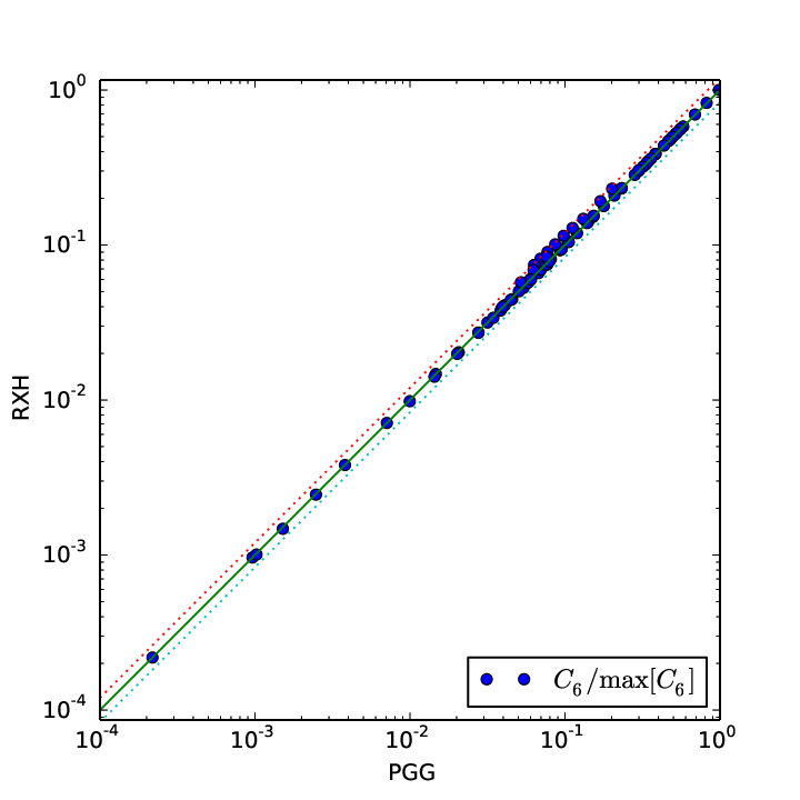
Refer to caption — Figure 1: Normalised RXH $C_{6}$ coefficients versus PGG values. The dotted lines indicate a difference of 20% between the two methods. Note that the worst outliers are all elements for which the rescaling parameter was interpolated based on neighbouring elements.

By using different TDDFT kernels we are able to provide a second test of the rescaling that incldues systems for which quantum chemical data are unavailable. Our test is based on the following idea: if rescaling can give good dynamic polarizabilities by correcting TDDFT calculations using static polarizabilities, then rescaled $C_{6}$ coefficients of different species should be largely independent of the exchange-correlation kernel employed in the TDDFT calculations. To test this hypothesis, we carried out calculations using two kernels: that of Petersilka-Gossman and GrossPetersilka et al. (1996), and the “radial exchange hole” kernel of GouldGould (2012). These two approaches give very different dipole polarizabilities before scaling, and can thus provide a clear test of the rescaling.

The results of our tests are plotted in Figure 1, in which rescaled RXH atomic $C_{6}$ coefficents are shown as a function of their PGG values. If all points fell perfectly on the straight line this would indicate that the rescaling was perfect, as two sets of inputs would have yielded the same set of $C_{6}$ coefficients after scaling. As it is, the values are all within 20% of each other, with the worst cases all being elements for which accurate reference polarizability values were not available and the rescaling parameters had to be interpolated based on other elements in the same row.

We thus conclude that starting with a moderately accurate TDDFT kernel, and then rescaling based on static dipole polarizabilities, is a very accurate approach for determining dynamic polarizabilities. Not only do we get good agreement with more accurate approaches, but we also get agreement across three TDDFT approaches: that of Chu and DalgarnoChu and Dalgarno (2004), and the two kernels tested here.

3 Results

Table 2: Static polarizabilities and

C_{6}

coefficients from the “benchmark” data set for all neutral atoms. We note that the small error in Hydrogen’s

C_{6}

coefficient of 13/2 is an artefact of the two-Lorentzian model. Results in

a_{0}^{3}

for polarizabilities and Ha

a_{0}^{6}

for

C_{6}

coefficients.

ID	$\alpha(0)$	$C_{6}$	ID	$\alpha(0)$	$C_{6}$	ID	$\alpha(0)$	$C_{6}$	ID	$\alpha(0)$	$C_{6}$	ID	$\alpha(0)$	$C_{6}$	ID	$\alpha(0)$	$C_{6}$
H	4.50	6.51	He	1.38	1.47
Li	164	1410	Be	37.7	214
B	20.5	99.2	C	11.7	47.9	N	7.25	25.7	O	5.20	16.7	F	3.60	10.2	Ne	2.67	6.91
Na	163	1570	Mg	71.4	629
Al	57.5	520	Si	37.0	308	P	24.8	187	S	19.5	140	Cl	14.7	97.1	Ar	11.1	67.4
K	290	3910	Ca	160	2230
Sc	123	1570	Ti	102	1200	V	87.3	955	Cr	78.4	709	Mn	66.8	635	Fe	60.4	548
Co	53.9	461	Ni	48.4	393	Cu	41.7	264	Zn	38.4	276
Ga	52.1	456	Ge	40.2	365	As	29.6	260	Se	26.2	233	Br	21.6	187	Kr	16.8	136
Rb	317	4660	Sr	198	3230
Y	163	2600	Zr	112	1360	Nb	97.9	1140	Mo	87.1	1030	Tc	79.6	939	Ru	72.3	809
Rh	66.4	708	Pd	61.7	628	Ag	46.2	341	Cd	46.7	405
In	62.1	643	Sn	60.0	715	Sb	44.0	504	Te	40.0	471	I	33.6	389	Xe	27.2	302
Cs	396	6660	Ba	278	5540	La	214	3730	Ce	205	3480	Pr	216	3760	Nd	209	3560
Pm	200	3340	Sm	192	3130	Eu	184	2940	Gd	158	2340	Tb	170	2590	Dy	163	2430
Ho	156	2280	Er	150	2150	Tm	144	2020	Yb	139	1910
Lu	137	2020	Hf	83.7	1040	Ta	73.9	887	W	65.8	757	Re	60.2	663	Os	55.3	584
Ir	51.3	522	Pt	48.0	470	Au	45.4	427	Hg	33.5	268
Tl	51.4	509	Pb	47.9	534	Bi	43.2	513	Po	36.1	424	At	30.4	351	Rn	32.2	408

Table 3: Static polarizabilities and

C_{6}

coefficients from the “benchmark” data set for all cations. Results in

a_{0}^{3}

for polarizabilities and Ha

a_{0}^{6}

for

C_{6}

coefficients.

ID	$\alpha(0)$	$C_{6}$	ID	$\alpha(0)$	$C_{6}$	ID	$\alpha(0)$	$C_{6}$	ID	$\alpha(0)$	$C_{6}$	ID	$\alpha(0)$	$C_{6}$	ID	$\alpha(0)$	$C_{6}$
He⁺	0.294	0.109	Li⁺	0.193	0.079
Be⁺	24.5	70.3	B⁺	9.67	25.2
C⁺	5.66	13.3	N⁺	3.68	8.02	O⁺	2.55	5.27	F⁺	1.78	3.44	Ne⁺	1.44	2.75	Na⁺	0.930	1.54
Mg⁺	35.0	155	Al⁺	19.6	89.7
Si⁺	18.2	94.8	P⁺	14.3	74.1	S⁺	11.9	62.2	Cl⁺	9.27	46.1	Ar⁺	7.28	34.2	K⁺	5.05	21.0
Ca⁺	75.5	554	Sc⁺	60.0	531
Ti⁺	44.6	286	V⁺	36.5	217	Cr⁺	38.2	236	Mn⁺	25.8	132	Fe⁺	23.2	114	Co⁺	20.6	95.8
Ni⁺	18.4	81.5	Cu⁺	17.6	75.9	Zn⁺	17.9	91.7	Ga⁺	15.2	71.8
Ge⁺	18.5	108	As⁺	16.4	102	Se⁺	15.7	104	Br⁺	13.6	91.2	Kr⁺	11.1	71.9	Rb⁺	8.32	49.1
Sr⁺	90.2	790	Y⁺	88.1	1020
Zr⁺	62.0	574	Nb⁺	55.3	512	Mo⁺	47.6	424	Tc⁺	32.7	246	Ru⁺	37.9	327	Rh⁺	34.4	284
Pd⁺	31.5	248	Ag⁺	20.0	115	Cd⁺	23.1	155	In⁺	20.2	127
Sn⁺	29.2	237	Sb⁺	25.5	215	Te⁺	25.1	230	I⁺	22.1	205	Xe⁺	18.7	170	Cs⁺	15.0	129
Ba⁺	121	1300	La⁺	94.2	1180	Ce⁺	89.1	1080	Pr⁺	93.4	1160	Nd⁺	89.6	1080	Pm⁺	85.7	1010
Sm⁺	81.8	941	Eu⁺	78.1	876	Gd⁺	67.2	698	Tb⁺	71.8	769	Dy⁺	68.6	717	Ho⁺	65.8	672
Er⁺	63.0	630	Tm⁺	60.4	590	Yb⁺	58.0	555	Lu⁺	74.6	808
Hf⁺	47.5	443	Ta⁺	42.0	388	W⁺	37.1	333	Re⁺	33.4	290	Os⁺	30.4	256	Ir⁺	27.9	228
Pt⁺	25.8	204	Au⁺	24.0	184	Hg⁺	17.5	114	Tl⁺	17.0	109
Pb⁺	23.5	185	Bi⁺	25.2	226	Po⁺	22.9	213	At⁺	20.2	190	Rn⁺	22.4	236

Table 4: Static polarizabilities and

C_{6}

coefficients from the “benchmark” data set for all anions. Results in

a_{0}^{3}

for polarizabilities and Ha

a_{0}^{6}

for

C_{6}

coefficients.

ID	$\alpha(0)$	$C_{6}$	ID	$\alpha(0)$	$C_{6}$	ID	$\alpha(0)$	$C_{6}$	ID	$\alpha(0)$	$C_{6}$	ID	$\alpha(0)$	$C_{6}$	ID	$\alpha(0)$	$C_{6}$
H^-	216	2400
Li^-	1180	35170
B^-	32.9	232	C^-	15.5	81.7	N^-	8.04	33.1	O^-	5.40	19.1	F^-	15.0	73.5
Na^-	1310	42690
Al^-	109	1550	Si^-	59.6	698	P^-	33.7	322	S^-	24.1	206	Cl^-	30.3	276
K^-	2090	87490
Sc^-	134	1860	Ti^-	110	1380	V^-	94.5	1100	Cr^-	83.5	908	Mn^-	74.7	762	Fe^-	66.5	640
Co^-	59.8	545	Ni^-	54.2	470	Cu^-	500	9440
Zn^-	845	17790	Ga^-	103	1430	Ge^-	63.3	796	As^-	40.0	443	Se^-	31.7	332	Br^-	42.8	497
Rb^-	2110	92240
Y^-	175	3080	Zr^-	134	2160	Nb^-	114	1680	Mo^-	100	1390	Tc^-	90.6	1170	Ru^-	82.4	1010
Rh^-	75.9	881	Pd^-	70.5	779	Ag^-	501	9800
Cd^-	863	20230	In^-	133	2240	Sn^-	89.1	1410	Sb^-	59.6	859	Te^-	49.1	684	I^-	61.7	925
Cs^-	2480	118890	La^-	729	19310	Ce^-	4.02	46.5	Pr^-	4.88	62.7	Nd^-	5.57	77.0	Pm^-	6.50	97.9
Sm^-	7.38	119	Eu^-	8.08	138	Gd^-	8.08	139	Tb^-	9.84	188	Dy^-	10.5	210	Ho^-	11.1	230
Er^-	11.6	246	Tm^-	12.0	260
Lu^-	13.8	325	Hf^-	236	4170	Ta^-	206	3640	W^-	295	5350	Re^-	368	6710	Os^-	378	6840
Ir^-	381	6830	Pt^-	383	6810	Au^-	387	6840
Tl^-	356	6820	Pb^-	135	2310	Bi^-	103	1710	Po^-	73.1	1140	At^-	54.5	801

We show in Tables 2-4 static polarizabilities and same-species $C_{6}$ coefficients using the “benchmark” data set of rescaled atoms and ions. These are arranged by shell structure to make for easy access. As discussed previously, these are in good agreement with external reference data and, for the most part, are in good agreement with RXH values. The exceptions show no more than a 15% difference, suggesting that this is a good estimate for the worst-case accuracy of our approach.

In addition to the tabulated static polarizabilities and $C_{6}$ coefficients, we also provide readily usable data for all cases considered here. Rather than provide tabulated frequency dependent polarizability data for all 411 atoms and ions (or 443 for the minimal chemistry model), we instead provide parameters $a_{c,X}$ and $\Omega_{c,X}$ where $c=1,2$ for a two Lorentzian model

\displaystyle\alpha_{X}(i\omega)\approx

\displaystyle\sum_{c=1,2}\frac{a_{c,X}}{\omega^{2}+\Omega_{c,X}^{2}},

(17)

for species $X$ with nuclear charge $Z$ and $N$ electrons. Eq. (17) can then be used to accurately reproduce the polarizabilities for arbitrary frequency.

This two-Lorentzian representation of polarizabilities can be used to reproduce all $C_{6}$ coefficients using analytic solutions of the Casimir-Polder formula (1) which take the form (here $X\equiv Z_{X},N_{X}$ and $Y\equiv Z_{Y}N_{Y}$ )

\displaystyle C_{6,XY}=

\displaystyle\sum_{cc^{\prime}}\frac{3a_{c,X}a_{c^{\prime},Y}}{2\Omega_{c,X}\Omega_{c^{\prime},Y}[\Omega_{c,X}+\Omega_{c^{\prime},Y}]}.

(18)

Results are within a few percent compared of similar calculations carried out on the raw data (see Appendix C for details). Our two-Lorentzian model thus provides a useful and compact representation for all dynamic polarizabilities, allowing reconstruction of the 84000+ different-species $C_{6}$ coefficients. These data are included in the supplementary materialSup (), tabulated for the “benchmark” set and included in ascii files for all data sets.

Table 5: Interaction of rare gas atoms with hailde atoms and ions and Na⁺. Results in Ha

a_{0}^{6}

	$C_{6}$ [Ref]	$C_{6}$ [this work]	% Err	Ref.
Br⁺–He	12.0	11.3	-5.8	Buchachenko et al. (2009)
Br–He	15.0	15.8	5.1	Buchachenko et al. (2009)
Br^-–He	27.0	24.0	-11.0	Buchachenko et al. (2009)
Br⁺–Ne	23.0	23.7	3.2	Buchachenko et al. (2009)
Br–Ne	31.0	32.8	5.8	Buchachenko et al. (2009)
Br^-–Ne	48.0	49.4	2.9	Buchachenko et al. (2009)
Br⁺–Ar	78.0	78.3	0.4	Buchachenko et al. (2009)
Br–Ar	110	111	0.9	Buchachenko et al. (2009)
Br^-–Ar	174	174	-0.3	Buchachenko et al. (2009)
Na⁺–He	1.79	1.39	-22.2	Soldán et al. (1999)
Na⁺–Ne	3.22	3.15	-2.2	Soldán et al. (1999)
Na⁺–Ar	10.4	8.71	-15.9	Soldán et al. (1999)
F^-–He	9.37	9.81	4.7	Hättig and Heß (1998)
F^-–Ne	19.4	20.5	5.6	Hättig and Heß (1998)
F^-–Ar	66.4	69.0	3.8	Hättig and Heß (1998)
F^-–Kr	95.2	98.9	3.9	Hättig and Heß (1998)
F^-–Xe	143	148	3.7	Hättig and Heß (1998)
F^-–Rn	170	172	1.4	Hättig and Heß (1998)
Cl^-–He	19.1	18.3	-4.0	Hättig and Heß (1998)
Cl^-–Ne	39.4	37.8	-4.1	Hättig and Heß (1998)
Cl^-–Ar	138	131	-4.8	Hättig and Heß (1998)
Cl^-–Kr	198	190	-4.3	Hättig and Heß (1998)
Cl^-–Xe	299	286	-4.3	Hättig and Heß (1998)
Cl^-–Rn	357	333	-6.7	Hättig and Heß (1998)
Br^-–He	24.0	24.0	0.2	Hättig and Heß (1998)
Br^-–Ne	49.4	49.4	-0.0	Hättig and Heß (1998)
Br^-–Ar	174	174	-0.3	Hättig and Heß (1998)
Br^-–Kr	251	251	0.0	Hättig and Heß (1998)
Br^-–Xe	380	380	0.1	Hättig and Heß (1998)
Br^-–Rn	452	443	-1.9	Hättig and Heß (1998)
I^-–He	32.1	32.1	-0.0	Hättig and Heß (1998)
I^-–Ne	65.9	65.8	-0.2	Hättig and Heß (1998)
I^-–Ar	233	233	-0.0	Hättig and Heß (1998)
I^-–Kr	336	338	0.5	Hättig and Heß (1998)
I^-–Xe	510	514	0.7	Hättig and Heß (1998)
I^-–Rn	608	599	-1.5	Hättig and Heß (1998)

We also test interactions of rare gas atoms with halides and the alkali cation Na⁺, to demonstrate the method’s capabilities on heteronuclear $C_{6}$ coefficients. We compare results from our data set against results from three references, and are thus able to cover elements in all of the six rows considered here. Results are presented in Table 5. Agreement is generally excellent, with a few cases substantially worse than the mean absolute relative error of 3.7%.

The worst relative errors all involve Na⁺ and rare gases. However, the absolute errors for these cases are small since neither Na⁺ nor rare gas atoms are very polarizable and the $C_{6}$ coefficients are consequently small. Also, the data from Ref. 48 may not be as accurate as more modern calculations would allow. The next worst case is Br^- with He when compared with the reference data of Ref. 47. Oddly, we get almost perfect agreement for this case with the (presumably less accurate) TDMP2 results of Ref. 49.

Finally, we use our comprehenesive data set to test for broad relationships between $C_{6}$ coefficients and static dipole polarizabilities $\alpha(0)$ . Based on units, one predicts that $C_{6,XY}\propto\alpha_{X}(0)\alpha_{Y}(0)$ might be a reasonable approximation for such a relationship. However, after testing all 3741 possible pairs of neutral atoms (plotted in Figure 2) we find that

\displaystyle C_{6,XY}\approx\Xi\big[\alpha_{X}(0)\alpha_{Y}(0)\big]^{0.73\pm 0.01},

(19)

$\Xi=(1.5\pm 0.1)$ [Ha $a_{0}^{1.62}$ ], is a better power law fit, showing a somewhat surprising reduction in the scaling coefficient from the expected product form. Here our parameter error bars are crudely estimated by comparing more limited fits with only same-species atomic and ionic coefficients, and all neutral atom pairs using our PGG and RXH data sets.

The constant prefactor $\Xi$ varies considerably depending on the data set selected, and Figure 2 makes it clear that the actual results have a much wider range of values. By contrast, the exponent $0.73\pm 0.01$ remains essentially constant. This suggests a certain universality of the power law relationship between polarizabilities and $C_{6}$ coefficients. We suspect that it might be possible to improve the quality of this fit by improving the dependence on $\alpha_{x}(0)$ and $\alpha_{y}(0)$ separately.

Along these lines, we test the quality of the relationship

\displaystyle C_{6,XY}=\frac{2C_{6,XX}C_{6,YY}}{\frac{\alpha_{X}(0)}{\alpha_{Y}(0)}C_{6,YY}+\frac{\alpha_{Y}(0)}{\alpha_{X}(0)}C_{6,XX}},

(20)

foundTang (1969) from a one-Lorentzian model $\alpha(i\omega)=\alpha(0)/(1+\omega^{2}/\eta^{2})$ (equivalent to the [1,0] Padé approximation for the polarizability). This has previously been used (e.g. Ref. 20) to derive different-species coefficients from same-species data. We find that (20) is generally very accurate, giving answers within 5% of our two-Lorentzian model (18) for almost 80% of cases (from 84000 pairs of atoms, anions and cations). However in 2.0% ( $\approx 1700$ ) of cases it is more than 20% out and in 0.2% ( $\approx 200$ ) of cases it is more than 30% out.

It should be noted that most of these worst case examples involve 2+ or 3+ cations interacting with an anion, and thus give rise to small absolute errors. None of the cases with $>20\%$ errors involve two neutral atoms. Some notable bad cases examples are Na⁺ with Cs (-21%), and Al^- with many anions in Row 6 ( $\approx-24\%$ ).

4 Conclusions

Using TDDFT with the PGGPetersilka et al. (1996) kernel we calculated all-electron dipole polarizabilities of all atoms and many cations and anions from rows 1-6 ( $1\leq Z\leq 86$ ) of the periodic table. We also performed calculations using an alternative RXHGould (2012) kernel; and using a variant method designed to approximate more realistic environmental effects for atoms in molecules, which yields different coefficients for open-shell anions. We argue that these dipole polarizabilities can provide a rough benchmark (likely within 15% for all species, with better results expected in some cases) for imaginary frequency dipole polarizability calculations of $C_{6}$ coefficients. They are almost certainly of sufficient quality to be used in atom-in-molecule (AIM) approaches, be they classical, semi-classical, or semi-empirical.

Our polarizabilities were parametrised using a two-Lorentzian model (17) that can be used to reproduce $C_{6}$ coefficients within 5% (and typically $<$ 1%) of the value obtained by full quadrature via the Casimir-Polder formula (1). These parameters were tabulated for all atoms and ions investigated, and are included in the supplementary materialsSup (). These were used to calculate homonuclear-isoelectronic $C_{6}$ coefficients and some heteronuclear coefficients.

We finally used our data to study the dependence of $C_{6}$ coefficients on polarizabilities, finding $C_{6,XY}\approx\Xi[\alpha_{X}(0)\alpha_{Y}(0)]^{0.73\pm 0.01}$ , with error bars indicating the spread of best-fit parameters found on different data sets. While the prefactor $\Xi$ was found to vary considerably depending on the data set used to make the fit, the exponent varied much less suggesting it is a more universal quantity. Similarly, we tested the relationship $C_{6,XY}=2C_{6,X}C_{6,Y}/[\alpha_{X}/\alpha_{Y}C_{6,Y}+\alpha_{Y}/\alpha_{X}C_{6,X}]$ sometimes used to relate homonuclear-isoelectronic coefficients and $C_{6}$ for pairs of unlike species (atoms or ions). We found that it gave errors of less than 5% in 80% of cases, but in 0.2% of cases gave very poor results with $>30$ % errors.

In future we also hope to use our approach to study atoms and ions in Row 7, after developing techniques to deal with relativistic effects and fixed core approximations. We also aim to explore other environmental effects to better understand how embedded atoms behave compared to their free counterparts, and thus to improve and extend the “minimal chemistry” model presently used to determine some cation and all double cation dipole polarizabilities.

TG recognises computing support from the Griffith University Gowonda HPC Cluster. TB acknowledges support from the project APVV-15-0105 and the use of computational resources of supercomputing infrastructure of Computing Center of the Slovak Academy of Sciences acquired in Project Nos. ITMS 26230120002 and 26210120002 supported by the Research and Development Operational Program funded by the ERDF. The authors thank Prof. Ivan Černušák for sharing accurate polarizability data for open-shell atoms and ions.

e include with this manuscript supporting information including:

A PDF document that includes: a) further details of the benchmark data set; b) several additional tables of chief results; c) a description of the accompanying ascii files;
Several ascii files presenting chief results in a readily usable format.

Appendix A Transition metal and lanthanide atoms and ions

Some of the transition metal and lanthanide atoms and ions represent very difficult casees for single-determinant theories like DFT and HF. In certain cases the $s$ and $d$ orbitals (or $d$ and $f$ orbitals) are so close to degenerate that the aufbau principle can be violated in the lowest energy configuration for DFT calculations (see e.g. Ref. 51 or Ref. 52 for discussion in a Hartree-Fock context). Despite the LEXX approximation including some multi-determinental characteristics via the ensemble DFT formalism it too is affected by these issues. Furthermore, the route of explicit symmetry breaking employed by Johnson et al is not available in our radial code.

This poses a particular challenge for polarizability problems as the effective Kohn-Sham gap $\epsilon_{l}-\epsilon_{h}$ (for lowest unoccupied $f_{l}=0$ and highest occupied $f_{h}>0$ KS orbitals) can become negative. Since this gap appears in the denominator of terms contributing to $\chi_{0}$ it leads to unphysical small frequency (real or imaginary) polarizabilities. In certain cases it gives negative bare polarizabilities (i.e. calcualated via (2) except with $\chi_{0}$ rather than $\chi$ ). While these problems are somewhat mitigated in the interacting response $\chi$ by the screening kernel $f_{\text{Hxc}}$ (e.g. our approach returns positive static polarizabilities for all species tested), it still contributes substantial errors to polarizabilities.

We are thus left with a dilemma: do we choose the lowest energy groundstate or choose a state that does not give negative transitions but is in a less realistic electronic configuration? We thus decide to simplify matters by filling the orbitals according to $(n+1)s^{2}(n)d^{m}$ , where $n=3$ or 4 (or equivalent for $d$ and $f$ orbitals). This leads to some differences from free atom calculations, especially in Cr and Mo which have clearly lower energies in their $(n+1)s^{1}(n)d^{5}$ states. However, as these elements usually appear as embedded ions we expect the practical effect to be minimal.

Appendix B Minimal chemistry model

The main purpose of this manuscript is to report reference polarizabilities and $C_{6}$ coefficients for free-standing atoms and ions (for ions with $N\leq Z+1$ ). However, polarizabilities are often desired for their utility in embedded atom/ion models - such as for high-level calculations using van der Waals dispersion corrections (e.g. Refs. 17; 18; 19; 20; 21; 22), or for (semi-)classical force-field models. We thus also report a slightly modified set of reference coefficients for this purpose.

Atoms and ions “embedded” in a larger system such as a molecule or material can behave very differently to their free-standing counterparts. Most notably, the surrounding environment of an anion has a substantial effect on the behaviour of its outermost electron(s). They are only very weakly bound in the free-standing case, with an asymptotic effective potential going to zero as $~r^{-3}$ . When embedded, the other electrons and nucleii will introduce an effective confining potential, which can be approximated [see e.g. Ref. 53] by a positve power law function of $r$ such as $(r/r_{a})^{\sigma_{a}}$ where $r_{a}$ is an effective embedding radius and $\sigma_{a}$ governs the sharpness. Clearly the energetics of the outermost orbital and unoccupied orbitals are very different in both cases.

But the same electrons that are most sensitive to the embedding environment, namely electrons in the outermost electronic shell(s), are the ones that contribute the most to the polarizibilty. Thus the polarizability of an embedded system is highly sensitive to its enviroment and care must be taken in considering what “anions” should be used in embedding theories. This is especially pertinent for open shell systems which are likely to be the most sensitive to the environment.

To account for embedding, we thus approximate embedded anions using a minimal chemistry model chosen to ensure that the “free” ions behave as closely as possible to their embedded counterparts without taking into account the full details of the chemical environment. To this end, we carry out polarizability calculations using a frozen orbital model, in which the polarizabilities $\alpha\equiv\alpha[v_{s}[v_{Z}],\{f_{i}\}]$ are treated (in TDDFT) as a functional of the interacting potential $v_{s}$ via $\chi[v_{s},\{f_{i}\},f_{\text{Hxc}}](\boldsymbol{r},\boldsymbol{r}^{\prime};i\omega)$ , discussed in detail just before Sec. 1.1.1. This allows us to introduce some embedding effects via our choice of $v_{s}$ arising from external potential $v_{Z}=-Z/r$ .

Our minimal chemistry model involves determining $v_{s}$ from the following rules:

1.

For neutral atoms and cations, find the atomic potential self-consistently using LEXX theory, Hund’s rules and the aufbau principle, (see Appendix A for further details on Rows 4-6) then rescale the polarizabilities using (15);
2.

For single anions A^- of halides ( $N=10,18,36,54,86$ , $Z=N-1$ ) calculate the ionic potential self-consistently using LEXX theory and then rescale (like for neutral atoms);
3.

For the remaining single anions A^- use the self-consistent LEXX potential of the neutral atom and do not rescale;
4.

For all double anions A^2- use the self-consistent LEXX potential of the neutral atom and do not rescale;

This method produces an alternative set of frequency dependent anionic polarizabilities that, we feel, may better reflect the reality of embedded anions. This alternative data set is provided in the supplementary dataSup ().

Appendix C Two-Lorentzian polarizability model

From equation (14)

\displaystyle\alpha(i\omega)\approx

\displaystyle\sum_{kl}\frac{d_{kl}}{(E_{k}-E_{l})^{2}+\omega^{2}}

(21)

it is clear that the imaginary frequency dependence of $\alpha$ is a sum over Lorentzian functions $d/(\omega^{2}+\Omega^{2})$ . In a typical atom one Lorentzian will typically have a denominator (the square of the lowest excitation energy + $\omega^{2}$ ) that is significantly smaller than the other terms for small $\omega$ , and thus dominates the $C_{6}$ coefficient. When combined with the known limit $\lim_{\omega\to\infty}\alpha(i\omega)=N/\omega^{2}$ (i.e. $\sum d_{kl}=N$ ) this suggests that a reduced number of Lorentzians should be sufficient to represent the imaginary frequency dipole polarizabilities.

In fact, our results suggest that $\alpha(i\omega)$ for atoms/ions can be approximated by just two Lorentzians with minimal loss of accuracy. Thus, for every atom and ion with nuclear charge $Z$ and electron number $N$ we write

\displaystyle\alpha_{X}(i\omega)\approx

\displaystyle\sum_{c=1,2}\frac{a_{c,X}}{\omega^{2}+\Omega_{c,X}^{2}}

(22)

without any great loss of accuracy. Here the parameters $a_{1}$ , $\Omega_{1}$ and $\Omega_{2}$ are varied to minimze $\int(\alpha-\alpha^{\text{Numeric}})^{2}d\omega$ while $a_{2}=N-a_{1}$ is kept fixed to ensure that the polarizability has the correct asymptote.

We note that Figari et alFigari et al. (2007); Figari and Magnasco (2007) have carefully studied similar pseudospectral methods to the one employed here. They showed that four Lorentzians are generally sufficient for very high accuracy and that careful treatment of the frequencies $\Omega_{c}$ can further improve results. However, given the merely “moderate” quality of our inputs, we feel that such an analysis would not offer meaningful benefits for our present work.

References

Dobson and Gould (2012) Dobson, J. F.; Gould, T. J. Phys: Condens. Matter 2012, 24, 073201.
Eshuis et al. (2012) Eshuis, H.; Bates, J. E.; Furche, F. Theor. Chem. Acc. 2012, 131, 1–18.
Ambrosetti et al. (2016) Ambrosetti, A.; Ferri, N.; DiStasio, R. A.; Tkatchenko, A. Science 2016, 351, 1171–1176.
Geim and Grigorieva (2013) Geim, A.; Grigorieva, I. Nature 2013, 499, 419–425.
Lebègue et al. (2010) Lebègue, S.; Harl, J.; Gould, T.; Ángyán, J. G.; Kresse, G.; Dobson, J. F. Phys. Rev. Lett. 2010, 105, 196401.
Björkman et al. (2012) Björkman, T.; Gulans, A.; Krasheninnikov, A. V.; Nieminen, R. M. Phys. Rev. Lett. 2012, 108, 235502.
Björkman et al. (2012) Björkman, T.; Gulans, A.; Krasheninnikov, A. V.; Nieminen, R. M. J. Phys: Condens. Matter 2012, 24, 424218.
Björkman (2014) Björkman, T. J. Chem. Phys. 2014, 141.
Gobre and Tkatchenko (2013) Gobre, V. V.; Tkatchenko, A. Nat. Commun. 2013, 4, 2341.
Perdew et al. (1996) Perdew, J. P.; Burke, K.; Ernzerhof, M. Phys. Rev. Lett. 1996, 77, 3865–3868.
Dobson et al. (2001) Dobson, J. F.; McLennan, K.; Rubio, A.; Wang, J.; Gould, T.; Le, H. M.; Dinte, B. P. Aust. J. Chem. 2001, 54, 513–527.
Dobson and Dinte (1996) Dobson, J. F.; Dinte, B. P. Phys. Rev. Lett. 1996, 76, 1780–1783.
Lundqvist et al. (1995) Lundqvist, B. I.; Andersson, Y.; Shao, H.; Chan, S.; Langreth, D. C. Int. J. Quantum Chem. 1995, 56, 247–255.
Andersson et al. (1996) Andersson, Y.; Langreth, D. C.; Lundqvist, B. I. Phys. Rev. Lett. 1996, 76, 102–105.
Dion et al. (2004) Dion, M.; Rydberg, H.; Schröder, E.; Langreth, D. C.; Lundqvist, B. I. Phys. Rev. Lett. 2004, 92, 246401.
Langreth et al. (2005) Langreth, D. C.; Dion, M.; Rydberg, H.; Schröder, E.; Hyldgaard, P.; Lundqvist, B. I. Int. J. Quantum Chem. 2005, 101, 599–610.
Grimme (2004) Grimme, S. J. Comput. Chem. 2004, 25, 1463–1473.
Grimme (2006) Grimme, S. J. Comput. Chem. 2006, 27, 1787–1799.
Grimme et al. (2010) Grimme, S.; Antony, J.; Ehrlich, S.; Krieg, H. J. Chem. Phys. 2010, 132, 154104.
Tkatchenko and Scheffler (2009) Tkatchenko, A.; Scheffler, M. Phys. Rev. Lett. 2009, 102, 073005.
Tkatchenko et al. (2012) Tkatchenko, A.; DiStasio, R. A.; Car, R.; Scheffler, M. Phys. Rev. Lett. 2012, 108, 236402.
DiStasio et al. (2012) DiStasio, R. A.; von Lilienfeld, O. A.; Tkatchenko, A. Proc. Natl. Acad. Sci. U. S. A. 2012, 109, 14791–14795.
Becke (1988) Becke, A. D. Phys. Rev. A 1988, 38, 3098–3100.
Lee et al. (1988) Lee, C.; Yang, W.; Parr, R. G. Phys. Rev. B 1988, 37, 785–789.
Bučko et al. (2014) Bučko, T.; Lebègue, S.; Ángyán, J. G.; Hafner, J. J. Chem. Phys. 2014, 141, 034114.
Bučko et al. (2016) Bučko, T.; Lebègue, S.; Gould, T.; Ángyán, J. G. J. Phys.: Condens. Matter 2016, 28, 045201.
Dobson (2014) Dobson, J. F. Int. J. Quantum Chem. 2014, 114, 1157–1161.
Mitroy et al. (2010) Mitroy, J.; Safronova, M. S.; Clark, C. W. J. Phys. B 2010, 43, 202001.
Schwerdtfeger (2006) Schwerdtfeger, P. In Computational Aspects of Electric Polarizability Calculations: Atoms, Molecules and Clusters,; Maroulis, G., Ed.; IOS Press, Amsterdam, 2006; Chapter Atomic Static Dipole Polarizabilities, pp 1–32., Updated static dipole polarizabilities are available as pdf file from the CTCP website at Massey University: http://ctcp.massey.ac.nz/dipole-polarizabilities.
Chu and Dalgarno (2004) Chu, X.; Dalgarno, A. J. Chem. Phys. 2004, 121, 4083–4088.
Axilrod and Teller (1943) Axilrod, B. M.; Teller, E. J. Chem. Phys. 1943, 11, 299–300.
Gould (2012) Gould, T. J. Chem. Phys. 2012, 137, 111101.
Gould and Dobson (2012) Gould, T.; Dobson, J. F. Phys. Rev. A 2012, 85, 062504.
Gould and Dobson (2013) Gould, T.; Dobson, J. F. J. Chem. Phys. 2013, 138, 014103.
Gould and Dobson (2013) Gould, T.; Dobson, J. F. J. Chem. Phys. 2013, 138, 014109.
Petersilka et al. (1996) Petersilka, M.; Gossmann, U. J.; Gross, E. K. U. Phys. Rev. Lett. 1996, 76, 1212–1215.
Krieger et al. (1992) Krieger, J. B.; Li, Y.; Iafrate, G. J. Phys. Rev. A 1992, 45, 101–126.
Zaremba and Kohn (1976) Zaremba, E.; Kohn, W. Phys. Rev. B 1976, 13, 2270 – 2285.
Sadlej and Urban (1991) Sadlej, A. J.; Urban, M. J. Mol. Struct.: THEOCHEM 1991, 234, 147 – 171.
Miadoková et al. (1997) Miadoková, I.; Kellö, V.; Sadlej, A. J. Theor. Chem. Acc. 1997, 96, 166–175.
Holka et al. (2005) Holka, F.; Neogrády, P.; Kellö, V.; Dierksen, M. U. U. H. F. Mol. Phys. 2005, 103, 2747–2761.
Thierfelder et al. (2008) Thierfelder, C.; Assadollahzadeh, B.; Schwerdtfeger, P.; Schäfer, S.; Schäfer, R. Phys. Rev. A 2008, 78, 052506.
Dzuba et al. (2014) Dzuba, V. A.; Kozlov, A.; Flambaum, V. V. Phys. Rev. A 2014, 89, 042507.
Jiang et al. (2015) Jiang, J.; Mitroy, J.; Cheng, Y.; Bromley, M. At. Data Nucl. Data Tables 2015, 101, 158–186.
Éhn and Černušák (2016) Éhn, L.; Černušák, I. 2016, Private communication.
(46) See supporting information.
Buchachenko et al. (2009) Buchachenko, A. A.; Wright, T. G.; Lee, E. P. F.; Viehland, L. A. J. Chem. Phys. A 2009, 113, 14431–14438, PMID: 19603766.
Soldán et al. (1999) Soldán, P.; Lee, E. P.; Wright, T. G. Mol. Phys. 1999, 97, 139–149.
Hättig and Heß (1998) Hättig, C.; Heß, B. A. J. Chem. Phys. 1998, 108, 3863–3870.
Tang (1969) Tang,K. T. Phys. Rev. 1969, 177, 108.
Johnson et al. (2007) Johnson, E. R.; Dickson, R. M.; Becke, A. D. J. Chem. Phys. 2007, 126, 184104–184104.
Koga et al. (1995) Koga, T.; Aoki, H.; Tatewaki, H. Theor. Chim. Acta 1995, 92, 281–295.
Patel and Varshni (2009) Patel, S. H.; Varshni, Y. P. In Theory of Confined Quantum Systems: Part One; Sabin, J., Brandas, E., Eds.; Elsevier, 2009; Vol. 57; Chapter 1, pp 1–24.
Figari et al. (2007) Figari, G.; Rui, M.; Costa, C.; Magnasco, V. Theor. Chem. Acc. 2007, 118, 107–112.
Figari and Magnasco (2007) Figari, G.; Magnasco, V. Comput. Lett. 2007, 3, 277–284.

C6C_{6} coefficients and dipole polarizabilities for all atoms and many ions in rows 1-6 of the periodic table

Abstract

1 Theory

1.1 TDDFT Methodology

1.1.1 Numerical convergence

1.2 Corrected TDDFT calculations

2 Benchmarking tests

3 Results

4 Conclusions

Appendix A Transition metal and lanthanide atoms and ions

Appendix B Minimal chemistry model

Appendix C Two-Lorentzian polarizability model

References

$C_{6}$ coefficients and dipole polarizabilities for all atoms and many ions in rows 1-6 of the periodic table