Efficient Summing over Sliding Windows

Denote $z\triangleq\left\lfloor\frac{W}{\left\lfloor 2W\epsilon+1\right\rfloor}\right\rfloor$. We prove the lemma by showing $2^{z}$ arrangements that must lead to different configurations. Consider the language of all concatenations of $z$ blocks of size $\left\lfloor 2W\epsilon+1\right\rfloor$, such that each block consists of only ones or only zeros:

Assume, by way of contradiction, that two different words

lead the algorithm to the same configuration. Denote the index of the last block that differs between $s^{1}$ and $s^{2}$ by $t\triangleq max\{\tau\mid w_{\tau}^{1}\neq w_{\tau}^{2}\}.$ Next, consider the sequences $s^{1}\cdot 0^{(t-1)\left\lfloor 2W\epsilon+1\right\rfloor}$ and $s^{2}\cdot 0^{(t-1)\left\lfloor 2W\epsilon+1\right\rfloor}.$ The algorithm must reach the same configuration after processing these sequences, even though the number of ones differs by $\left\lfloor 2W\epsilon+1\right\rfloor>2W\epsilon$. Therefore, the algorithm’s error must be greater than $W\epsilon$ at least for one of the sequences, in contradiction to the assumption. We have shown $2^{z}$ words that lead to different configurations and therefore any deterministic algorithm that provides $\epsilon-additive$ approximation to Basic-Counting must have at least $z$ bits of state.    

Assume that some algorithm $A$ gives a $W\epsilon$-additive approximation using $m$ memory bits. Consider $A$’s run on the sequence $s=0^{W}\cdot 1^{2^{m}}$. Since $A$ is using $m$ bits, it reaches some memory configuration $c$ at least twice after processing the zeros in the sequence. Assume that $A$ first reached $c$ after seeing $0^{W}\cdot 1^{y}$ (where $y<2^{m}$). This means that $A$ must output some number $a_{c}\leq y+W\epsilon$ if queried. Now assume $A$ returns to configuration $c$ after reading $z$ additional ones. This means $A$ will return to $c$ after every additional sequence of $z$ ones. Therefore, for every integer $q$, after processing the sequence $0^{W}\cdot 1^{y+qz}$, $A$ will reach configuration $c$. We can then pick a large $q$ (such that $y+qz\geq W$), which means that the query answer for configuration $c$, $a_{c}$, has to be at least $W(1-\epsilon)$, as the window is now all-ones. We get $W(1-\epsilon)\leq a_{c}\leq y+W\epsilon$ and thus $2^{m}>y\geq W(1-2\epsilon)$. Putting everything together, we conclude that $m>\log\left(W(1-2\epsilon)\right)=\log W+\log\left(1-2\epsilon\right)\geq\log W-1$, for $\epsilon\leq\frac{1}{4}$. Finally, since $m$ is an integer, this implies $m\geq\left\lfloor{\log W}\right\rfloor$.    

Immediate from lemmas 3 and 4.    

We say that algorithm $A$ is $\epsilon$-correct on a input instance $S$ if it is able to approximate the number of $1$’s in the last $W$ bits, at every time instant while reading $S$, to within an additive error of $W\epsilon$.

We remind the reader that in our case, a Las Vegas (LV) algorithm for the Basic-Counting approximation problem is a randomized algorithm which is always $\epsilon$-correct. In contrast, a Monte Carlo (MC) algorithm is a randomized procedure that is allowed to provide approximation with error larger than $W\epsilon$, with probability at most $\delta$.

The Yao Minimax principle [23] implies that the amount of memory required for a deterministic algorithm to approximate a random input chosen according to a distribution $\mathbf{p}$ is a lower bound on the expected space consumption of a Las Vegas algorithm for the worst input. To prove a $\left\lfloor{\frac{1}{2\epsilon+W^{-1}}}\right\rfloor$ lower bound, we consider padding the language $L_{W,\epsilon}$ which is defined in Lemma 3. Specifically, we define $\mathbf{p}$ as the uniform distribution over all inputs in the language

That is, the input consist of all bit sequences in $L_{W,\epsilon}$, followed by a sequence of $W$ zeros. The trailing $0$’s are used to force the algorithm to reach distinct configurations after reading the first $W$ input bits. As implied by the lemma, any deterministic algorithm which is always correct for a random instance requires at least $\left\lfloor{\frac{1}{2\epsilon+W^{-1}}}\right\rfloor$ bits, as it has to arrive to a distinct state for each input $s\in L_{W,\epsilon}$. The argument for a lower bound of $\left\lfloor{\log W}\right\rfloor$ bits is similar.

Next, we use the Minimax principle analogue for Monte Carlo algorithms [23], which states that for any input distribution $\mathbf{p}$ and $\delta\in[0,1/2]$, any randomized algorithm that is always (for any input) $\epsilon$-correct with probability at least $1-\delta$ uses in expectation at least half as much memory as the optimal deterministic algorithm that errs (i.e., is not $\epsilon$-correct) with probability at most $2\delta$ on a random instance drawn according to $\mathbf{p}$. Once again, we consider $\mathbf{p}$ to be the uniform distribution over

Since the distribution is uniform, any deterministic algorithm, which is $\epsilon$-correct with probability at least $1-2\delta$ on a random instance drawn according to $\mathbf{p}$, is actually $\epsilon$-correct on $1-2\delta$ fraction of the inputs. Similar to the LV case, the argument in Lemma 3 implies that the algorithm must reach a distinct configuration after reading the first $W$ bits of each of the $(1-2\delta)\cdot|L_{MC}|$ inputs it is $\epsilon$-correct on. Consequently, the algorithm must use at least $\log\left({(1-2\delta)\cdot|L_{MC}|}\right)$ bits of memory. Applying the Minimax principle, the derived lower bound $B_{MC}$ for any MC algorithm is:

Once again, the case for a $\Omega(\log W)$ lower bound is based on Lemma 4 and follows from similar arguments.    

First, let us introduce some notations used in the proof. Assume that the index of the last bit is $W+m$, where $x_{W}$ is the last bit of a block and $m<{W\over k}$. $b_{i}$ is considered after $W+m$ bits have been processed. We denote $y_{j}$ the value of $y$ after adding bit $j$.

The setting for the proof is given in Figure 1. We aim to approximate

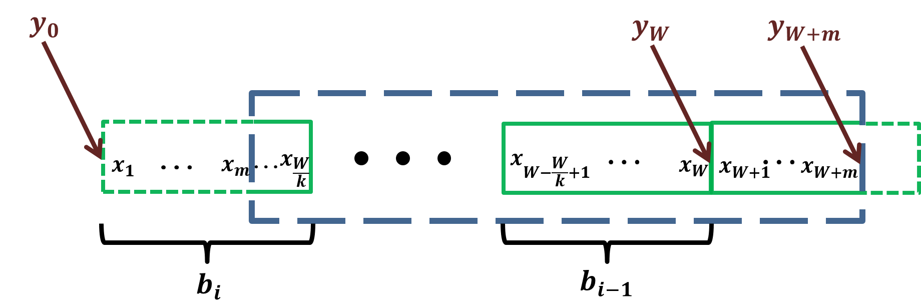
Our algorithm uses the following approximation:

At times $1,2,\ldots,W$, $y$ is incremented once for every set bit in the input stream. At the end of block $j$, if $y$ is reduced by $\frac{W}{k}$, then $b_{j}$ is set and will not be cleared before time $W+m$. Therefore, $\frac{W}{k}\cdot B+y_{W}=y_{0}+\sum_{j=1}^{W}x_{j}.$ Substituting $\frac{W}{k}\cdot B+y_{W}$ in (2), we get

We have established that in all cases the absolute error is at most $W\epsilon$ as required.    

We represent $y$ using $\left\lceil 2+\log(W\epsilon)\right\rceil$ bits, $m$ using $\left\lceil 1+log(W\epsilon)\right\rceil$ bits and $b$ using $k$ bits. Additionally, $i$ requires $\lceil\log k\rceil$ bits, and $B$ another $\lceil\log(k+1)\rceil$ bits. Overall, the number of bits required is $k+\left\lceil 2+\log(W\epsilon)\right\rceil+\left\lceil 1+\log(W\epsilon)\right\rceil+\lceil\log k\rceil+\lceil\log(k+1)\rceil\\ \leq k+2\log(W\epsilon)-2\log(2\epsilon)+8=\frac{1}{2\epsilon}+2\log(W)+6=\frac{1}{2\epsilon}+2\log W+O(1).$    

The proof of the lemma is very similar to the proof of Theorem 5 and is obtained by replacing every set bit with the integer $R$ in Lemma 3 and Lemma 4.    

Denote $x\triangleq\left\lfloor{2RW\epsilon+1}\right\rfloor$ and $C\triangleq\left\{n\cdot x\mid n\in\left\{0,1,\ldots,\left\lfloor{\frac{1}{2W\epsilon+R^{-1}}}\right\rfloor\right\}\right\}$. Let $L$ be the language of all $W$ length strings over the number in $C$, i.e.,

We show that every two distinct sequences in $L$ must lead the algorithm into distinct configurations implying a lower bound of

bits, where the last inequality follows from the fact that any $\epsilon<\frac{1}{2RW}$ implies exact summing. Assume, by way of contradiction, that two different words

lead the algorithm to the same configuration. Denote the index of the last letter that differs between $s^{1}$ and $s^{2}$ by $t\triangleq max\{\tau\mid\sigma_{\tau}^{1}\neq\sigma_{\tau}^{2}\}.$ Next, consider the sequences $s^{1}\cdot 0^{t-1}$ and $s^{2}\cdot 0^{t-1}.$ The algorithm must reach the same configuration after processing these sequences, even though the sum of the last $W$ elements differ by at least $x=\left\lfloor{2RW\epsilon+1}\right\rfloor>2RW\epsilon$. Therefore, the algorithm’s error must be greater than $RW\epsilon$ at least for one of the sequences, in contradiction to the assumption.    

Lemma 11 shows that approximating Basic-Summing within $RW\epsilon$ requires

bits for $\frac{1}{2W}\leq\epsilon\leq\frac{1}{4}.$ The same argument used in Lemma 9 shows that this implies $\Omega\left({\frac{1}{\epsilon}+\log W}\right)$ bits lower bound for any $\epsilon\geq\frac{1}{2W}$. For $\epsilon<\frac{1}{2W}$ such that $\epsilon=\Theta(W^{-1})$, approximating Basic-Summing within $RW\epsilon$ implies a $\frac{R}{2}$-additive approximation and therefore the $\Omega\left({\frac{1}{\epsilon}+\log W}\right)$ bound holds. For $\epsilon=o\left({\frac{1}{W}}\right)$, we use Lemma 12, which implies a lower bound of $W\log\left\lfloor{\frac{1}{4W\epsilon}+1}\right\rfloor=\Omega\left({W\log\left({\frac{1}{W\epsilon}}\right)}\right)$ memory bits.

References

- [1] Lee, L. K. and Ting, H. F. A Simpler and More Efficient Deterministic Scheme for Finding Frequent Items over Sliding Windows, Proceedings of the Twenty-fifth ACM SIGMOD-SIGACT-SIGART Symposium on Principles of Database Systems (PODS) 2006.
- [2] Albert, M.H., Golynski, A., Hamel, A.M., Lopez-Ortiz, A., Rao, S.S., Safari, M.A.: Longest increasing subsequences in sliding windows. Theoretical Comp. Sci. 321(2), 405-414 (2004)
- [3] Arasu, A., Manku, G.S.: Approximate counts and quantiles over sliding windows. In: Pro- ceedings of the 23rd ACM SIGACT-SIGMOD-SIGART Symposium on Principles of Database Systems, (PODS) 2004.
- [4] Babcock, B., Datar, M., Motwani, R., O’Callaghan, L.: Maintaining variance and k-medians over data stream windows. In: Neven, F., Beeri, C., Milo, T. (eds.) Proceedings of the Twenty- Second ACM SIGACT-SIGMOD-SIGART Symposium on Principles of Database Systems, June 9-12, 2003, San Diego, CA, USA. pp. 234-243. ACM (2003)
- [5] Ben Basat, R., Einziger, G., Friedman, R., Kassner, Y.: Heavy Hitters in Streams and Sliding Windows. In: Proc. IEEE INFOCOM, 2016.
- [6] Braverman, V., Gelles, R., Ostrovsky, R.: How to catch l2-heavy-hitters on sliding windows. Theoretical Computer Science 554, 82-94 (2014)
- [7] Braverman, V., Ostrovsky, R.: Smooth histograms for sliding windows. In: Foundations of Computer Science, 2007. FOCS’07. 48th Annual IEEE Symposium on. pp. 283-293.
- [8] Cohen, E., Strauss, M.J.: Maintaining time-decaying stream aggregates. J. Algorithms 59(1), 19-36 (2006)
- [9] Cormode, G., Yi, K.: Tracking distributed aggregates over time-based sliding windows. In: Scientific and Statistical Database Management. pp. 416-430. Springer (2012)
- [10] Crouch, M., Stubbs, D.S.: Improved streaming algorithms for weighted matching, via un- weighted matching. In: Approximation, Randomization, and Combinatorial Optimization. Al- gorithms and Techniques, APPROX/RANDOM 2014, September 4-6, 2014, Barcelona, Spain. pp. 96-104 (2014), http://dx.doi.org/10.4230/LIPIcs.APPROX-RANDOM.2014.96
- [11] Crouch, M.S., McGregor, A., Stubbs, D.: Dynamic graphs in the sliding-window model. In: Algorithms-ESA 2013, pp. 337-348. Springer (2013)
- [12] Datar, M., Gionis, A., Indyk, P., Motwani, R.: Maintaining stream statistics over sliding windows. SIAM J. Comput. 31(6), 1794-1813 (2002)
- [13] Gibbons, P.B., Tirthapura, S.: Distributed streams algorithms for sliding windows. In: SPAA. pp. 63-72 (2002)
- [14] Hung, R., Ting, H.: Finding heavy hitters over the sliding window of a weighted data stream. In: Laber, E., Bornstein, C., Nogueira, L., Faria, L. (eds.) LATIN 2008: Theoretical Informatics, LNCS , vol. 4957, pp. 699-710. Springer Berlin Heidelberg (2008)
- [15] Lee, L., Ting, H.F.: Maintaining significant stream statistics over sliding windows. In: Proceedings of the Seventeenth Annual ACM-SIAM Symposium on Discrete Algorithms, SODA 2006, Miami, Florida, USA, January 22-26, 2006. pp. 724-732. ACM Press (2006)
- [16] Liu, Y., Chen, W., Guan, Y.: Near-optimal approximate membership query over time-decaying windows. In: INFOCOM, 2013 Proceedings IEEE. pp. 1447-1455 (April 2013)
- [17] Mouratidis, K., Bakiras, S., Papadias, D.: Continuous monitoring of top-k queries over sliding windows. In: Proceedings of the 2006 ACM SIGMOD International Conference on Management of Data. pp. 635-646. SIGMOD ’06, ACM, New York, NY, USA (2006)
- [18] Naor, M., Yogev, E.: Sliding bloom filters. In: Cai, L., Cheng, S.W., Lam, T.W. (eds.) Algorithms and Computation, Lecture Notes in Computer Science, vol. 8283, pp. 513-523. Springer Berlin Heidelberg (2013)
- [19] Pripuzic, K., Zarko, I.P., Aberer, K.: Time- and space-efficient sliding window top-k query processing. ACM Trans. Database Syst. 40(1), 1:1-1:44 (Mar 2015)
- [20] Shen, H., Zhang, Y.: Improved approximate detection of duplicates for data streams over sliding windows. Journal of Computer Science and Technology 23(6), 973-987 (2008)
- [21] Shen, Z., Cheema, M., Lin, X., Zhang, W., Wang, H.: Efficiently monitoring top-k pairs over sliding windows. In: Data Engineering (ICDE), 2012 IEEE 28th International Conference on. pp. 798-809 (April 2012)
- [22] Zhang, W., Zhang, Y., Cheema, M.A., Lin, X.: Counting distinct objects over sliding windows. In: Proceedings of the Twenty-First Australasian Conference on Database Technologies - Volume 104. pp. 75-84. ADC ’10, Australian Computer Society, Inc., Darlinghurst, Australia, Australia (2010).
- [23] Yao AC. Probabilistic computations: Toward a unified measure of complexity. In Foundations of Computer Science, 1977, 18th Annual Symposium on 1977 (pp. 222-227). IEEE.
Appendix A Proof of Lemma 9
Proof.
We make a simple case analysis to show that the above holds:
- :
-
In this case the maximum in the denominator is . Hence
In this case, the maximum in the denominator is . Hence
An analysis of the function
reveals that it has a single extremum for positive s, located at . We check the value of the function at the extremum and at its boundaries:
This is a boundary because means that the algorithm is required to give an exact counting of the number of ones. On this boundary we get
- The extremum :
Appendix B Proof of Theorem 14
The case for bits when is similar to Theorem 6. The bound is obtained by replacing every set bit with the integer in the corresponding languages. In case , we consider the padded language obtained by adding ’s to every word in the language defined in Lemma 12. Further, we define the distribution to be uniform over
Similarly to Theorem 6, Lemma 12 implies that for (at least) fraction of the inputs in , the algorithm must reach a distinct state after reading the first integers. Therefore, the derived lower bound according to Yao’s Minimax principle [23] is:
Appendix C Proof of Theorem 15