跳到论文正文
W Papers独立论文阅读器 arXiv:1604.02199 论文正文 计算阅读时间 · 0%
引用这篇论文根据当前论文元数据生成,正式投稿前建议核对。


License: arXiv.org perpetual non-exclusive license
arXiv:1604.02199v3 [math.OC] 30 Apr 2022
\NatBibNumeric
\MSCCLASS

Primary: 90C15; secondary: 90C46 \ORMSCLASSPrimary: programming: stochastic

Distributionally Robust Stochastic Optimization with Wasserstein Distance

Rui Gao    Anton J. Kleywegt
Abstract

Distributionally robust stochastic optimization (DRSO) is an approach to optimization under uncertainty in which, instead of assuming that there is a known true underlying probability distribution, one hedges against a chosen set of distributions. In this paper we first point out that the set of distributions should be chosen to be appropriate for the application at hand, and that some of the choices that have been popular until recently are, for many applications, not good choices. We next consider sets of distributions that are within a chosen Wasserstein distance from a nominal distribution. Such a choice of sets has two advantages: (1) The resulting distributions hedged against are more reasonable than those resulting from other popular choices of sets. (2) The problem of determining the worst-case expectation over the resulting set of distributions has desirable tractability properties. We derive a strong duality reformulation of the corresponding DRSO problem and construct approximate worst-case distributions (or an exact worst-case distribution if it exists) explicitly via the first-order optimality conditions of the dual problem.

Our contributions are four-fold. (i) We identify necessary and sufficient conditions for the existence of a worst-case distribution, which are naturally related to the growth rate of the objective function. (ii) We show that the worst-case distributions resulting from an appropriate Wasserstein distance have a concise structure and a clear interpretation. (iii) Using this structure, we show that data-driven DRSO problems can be approximated to any accuracy by robust optimization problems, and thereby many DRSO problems become tractable by using tools from robust optimization. (iv) Our strong duality result holds in a very general setting. As examples, we show that it can be applied to infinite dimensional process control and intensity estimation for point processes.

keywords
distributionally robust optimization; Wasserstein metric; data-driven decision-making; ambiguity set; worst-case distribution
††authors: Department of Information, Risk and Operations Management, University of Texas at Austin, Austin, TX 78705, rui.gao@mccombs.utexas.edu H. Milton Stewart School of Industrial and Systems Engineering, Georgia Institute of Technology, Atlanta, GA 30332, anton@isye.gatech.edu ††affiliation: ††affiliation: ††affiliation: ††affiliation:

1 Introduction

In decision making problems under uncertainty, a decision maker wants to choose a decision xx from a feasible region XX. The objective function Ψ:X×Ξ↦ℝ\Psi:X\times\Xi\mapsto\mathbb{R} depends on a quantity ξ∈Ξ\xi\in\Xi whose value is not known to the decision maker at the time that the decision has to be made. In some settings it is reasonable to assume that ξ\xi is a random element with distribution μ\mu supported on Ξ\Xi, for example, if multiple realizations of ξ\xi will be encountered. In such settings, the decision making problems can be formulated as stochastic optimization problems as follows:

infx∈X𝔼μ​[Ψ⁡(x,ξ)].\inf_{x\in X}\mathbb{E}_{\mu}[\Psi(x,\xi)].

We refer to Shapiro et al. [47] for a thorough study of stochastic optimization. One major criticism of the formulation above for practical applications is the requirement that the underlying distribution μ\mu be known to the decision maker. Even if multiple realizations of ξ\xi are observed, μ\mu still may not be known exactly, while use of a distribution different from μ\mu may sometimes result in bad decisions. Another major criticism is that in many applications there are not multiple realizations of ξ\xi that will be encountered, for example in problems involving events that may either happen once or not happen at all, and thus the notion of a “true” underlying distribution does not apply. These criticisms motivate the notion of distributionally robust stochastic optimization (DRSO), that does not rely on the notion of a known true underlying distribution. One chooses a set 𝔐\mathfrak{M} of probability distributions to hedge against, and then finds a decision that provides the best hedge against the set 𝔐\mathfrak{M} of distributions by solving the following minmax problem:

infx∈Xsupμ∈𝔐𝔼μ​[Ψ⁡(x,ξ)].\inf_{x\in X}\sup_{\mu\in\mathfrak{M}}\mathbb{E}_{\mu}[\Psi(x,\xi)]. (DRSO)

Such a minmax approach has its roots in Von Neumann’s game theory and has been used in many fields such as inventory management (Scarf et al. [45], Gallego and Moon [25]), statistical decision analysis (Berger [9]), as well as stochastic optimization (Žáčková [56], Dupačová [20], Shapiro and Kleywegt [48]). Recently it regained attention in the operations research literature, and sometimes is called data-driven stochastic optimization or ambiguous stochastic optimization.

A central question is: how to choose a good set of distributions 𝔐\mathfrak{M} to hedge against? A good choice of 𝔐\mathfrak{M} should take into account the properties of the practical application as well as the tractability of problem (DRSO). Two typical ways of constructing 𝔐\mathfrak{M} are moment-based and distance-based. The moment-based approach considers distributions whose moments (such as mean and covariance) satisfy certain conditions (Scarf et al. [45], Delage and Ye [19], Popescu [43], Zymler et al. [58]). It has been shown that in many cases the resulting DRSO problem can be formulated as a conic quadratic or semi-definite program. However, the moment-based approach is based on the curious assumption that certain conditions on the moments are known exactly but that nothing else about the relevant distribution is known. More often in applications, either one has data from repeated observations of the quantity ξ\xi, or one has no data, and in both cases the moment conditions do not describe exactly what is known about ξ\xi. In addition, the resulting worst-case distributions sometimes yield overly conservative decisions (Wang et al. [52], Goh and Sim [29]). For example, Wang et al. [52] shows that for the newsvendor problem, by hedging against all the distributions with fixed mean and variance, Scarf’s moment approach yields a two-point worst-case distribution, and the resulting decision does not perform well under other more likely scenarios.

The distance-based approach considers distributions that are close, in the sense of a chosen statistical distance, to a nominal distribution ν\nu, such as an empirical distribution or a Gaussian distribution (El Ghaoui et al. [21], Calafiore and El Ghaoui [16]). Popular choices of the statistical distance are ϕ\phi-divergences (Bayraksan and Love [6], Ben-Tal et al. [7]), which include Kullback-Leibler divergence (Jiang and Guan [32]), Burg entropy (Wang et al. [52]), and Total Variation distance (Sun and Xu [49]) as special cases, Prokhorov metric (Erdoğan and Iyengar [22]), and Wasserstein distance (Wozabal [53], Wozabal [54], Esfahani and Kuhn [23], Zhao and Guan [57]).

1.1 Motivation: Potential Issues with ϕ\phi-divergence

Despite its widespread use, ϕ\phi-divergence has a number of shortcomings. Here we highlight some of these shortcomings. In a typical setup using ϕ\phi-divergence, Ξ\Xi is partitioned into B¯+1\bar{B}+1 bins represented by points ξ0,ξ1,…,ξB¯∈Ξ\xi^{0},\xi^{1},\ldots,\xi^{\bar{B}}\in\Xi. The nominal distribution ν\nu associates NiN_{i} observations with bin ii. That is, the nominal distribution is given by ν:=(N0/N,N1/N,…,NB¯/N)\nu\vcentcolon=(N_{0}/N,N_{1}/N,\ldots,N_{\bar{B}}/N), where N:=∑i=0B¯NiN\vcentcolon=\sum_{i=0}^{\bar{B}}N_{i}. Let ΔB¯:={(p0,p1,…,pB¯)∈ℝ+B¯+1:∑j=0B¯pj=1}\Delta_{\bar{B}}\vcentcolon=\{(p_{0},p_{1},\ldots,p_{\bar{B}})\in\mathbb{R}_{+}^{{\bar{B}}+1}\,:\,\sum_{j=0}^{\bar{B}}p_{j}=1\} denote the set of probability distributions on the same set of bins. Let ϕ:[0,∞)↦ℝ\phi:[0,\infty)\mapsto\mathbb{R} be a chosen convex function such that ϕ⁡(1)=0\phi(1)=0, with the conventions that 0​ϕ​(a/0):=a​limt→∞ϕ⁡(t)/t0\phi(a/0)\vcentcolon=a\lim_{t\to\infty}\phi(t)/t for all a>0a>0, and 0​ϕ​(0/0):=00\phi(0/0)\vcentcolon=0. Then the ϕ\phi-divergence between μ=(p0,…,pB),ν=(q0,…,qB)∈ΔB¯\mu=(p_{0},\ldots,p_{B}),\nu=(q_{0},\ldots,q_{B})\in\Delta_{\bar{B}} is defined by

Iϕ​(μ,ν):=∑j=0B¯qj​ϕ​(pjqj).I_{\phi}(\mu,\nu)\ \ \vcentcolon=\ \ \sum_{j=0}^{\bar{B}}q_{j}\phi\left(\frac{p_{j}}{q_{j}}\right).

Let θ>0\theta>0 denote a chosen radius. Then 𝔐ϕ:={μ∈ΔB¯:Iϕ​(μ,ν)≤θ}\mathfrak{M}_{\phi}\vcentcolon=\left\{\mu\in\Delta_{\bar{B}}\,:\,I_{\phi}(\mu,\nu)\leq\theta\right\} denotes the set of probability distributions given by the chosen ϕ\phi-divergence and radius θ\theta. The DRSO problem corresponding to the ϕ\phi-divergence ball 𝔐ϕ\mathfrak{M}_{\phi} is then given by

infx∈Xsupμ∈ΔB¯{∑j=0B¯pj​Ψ​(x,ξj):Iϕ​(μ,ν)≤θ}.\inf_{x\in X}\sup_{\mu\in\Delta_{\bar{B}}}\left\{\sum_{j=0}^{\bar{B}}p_{j}\Psi(x,\xi^{j})\;:\;I_{\phi}(\mu,\nu)\leq\theta\right\}.

It has been shown in Ben-Tal et al. [7] that the ϕ\phi-divergence ball 𝔐ϕ\mathfrak{M}_{\phi} can be viewed as a statistical confidence region (Pardo [40]), and for several choices of ϕ\phi, the inner maximization of the problem above is tractable.

One well-known shortcoming of ϕ\phi-divergence balls is that, either they are not rich enough to contain distributions that are often relevant, or they they hedge against many distributions that are too extreme. For example, for some choices of ϕ\phi-divergence such as Kullback-Leibler divergence, if the nominal qi=0q_{i}=0, then pi=0p_{i}=0, that is, the ϕ\phi-divergence ball includes only distributions that are absolutely continuous with respect to the nominal distribution ν\nu, and thus does not include distributions with support on points where the nominal distribution ν\nu is not supported. As a result, if Ξ=ℝK\Xi=\mathbb{R}^{K} and ν\nu is discrete, then there are no continuous distributions in the ϕ\phi-divergence ball 𝔐ϕ\mathfrak{M}_{\phi}. Some other choices of ϕ\phi-divergence exhibit in some sense the opposite behavior. For example, the Burg entropy ball includes distributions with some amount of probability allowed to be shifted from ν\nu to any other bin, with the amount of probability allowed to be shifted depending only on θ\theta and not on how extreme the bin is. See Section 5.1 for more details regarding this potential shortcoming.

Next we illustrate another shortcoming of ϕ\phi-divergence that will motivate the use of Wasserstein distance.

Example 1.1

Suppose that there is an underlying true image (1b), and a decision maker possesses, instead of the true image, an approximate image (1a) obtained with a less than perfect device that loses some of the contrast. The images are summarized by their gray-scale histograms. (In fact, (1a) was obtained from (1b) by a low-contrast intensity transformation (Gonzalez and Woods [30]), by which the black pixels become somewhat whiter and the white pixels become somewhat blacker. This type of transformation changes only the gray-scale value of a pixel and not the location of a gray-scale value, and therefore it can also be regarded as a transformation from one gray-scale histogram to another gray-scale histogram.) As a result, roughly speaking, the observed histogram ν\nu is obtained by shifting the true histogram μt​r​u​e\mu_{true} inwards. Also consider the pathological image (1c) that is too dark to see many details, with histogram μp​a​t​h​o​l\mu_{pathol}. Suppose that the decision maker constructs a Kullback-Leibler (KL) divergence ball 𝔐ϕK​L:={μ∈ΔB¯:IϕK​L​(μ,ν)≤θ}\mathfrak{M}_{\phi_{KL}}\vcentcolon=\{\mu\in\Delta_{\bar{B}}\,:\,I_{\phi_{KL}}(\mu,\nu)\leq\theta\}. Note that IϕK​L​(μt​r​u​e,ν)=5.05>IϕK​L​(μp​a​t​h​o​l,ν)=2.33I_{\phi_{KL}}(\mu_{true},\nu)=5.05>I_{\phi_{KL}}(\mu_{pathol},\nu)=2.33. Therefore, if θ\theta is chosen small enough (less than 2.332.33) for 𝔐ϕK​L\mathfrak{M}_{\phi_{KL}} to exclude the pathological image (1c), then 𝔐ϕK​L\mathfrak{M}_{\phi_{KL}} will also exclude the true image (1b). If θ\theta is chosen large enough (greater than 5.055.05) for 𝔐ϕK​L\mathfrak{M}_{\phi_{KL}} to include the true image (1b), then 𝔐ϕK​L\mathfrak{M}_{\phi_{KL}} also has to include the pathological image (1c), and then the resulting decision may be overly conservative due to hedging against irrelevant distributions. If an intermediate value is chosen for θ\theta (between 2.332.33 and 5.055.05), then 𝔐ϕK​L\mathfrak{M}_{\phi_{KL}} includes the pathological image (1c) and excludes the true image (1b). In contrast, note that the Wasserstein distance W1W_{1} satisfies W1​(μt​r​u​e,ν)=30.7<W1​(μp​a​t​h​o​l,ν)=84.0W_{1}(\mu_{true},\nu)=30.7<W_{1}(\mu_{pathol},\nu)=84.0, and thus Wasserstein distance does not exhibit the problem encountered with KL divergence (see also Example 2.4).

Refer to caption
(a) Observed image with histogram ν\nu
Refer to caption
(b) True image with histogram μt​r​u​e\mu_{true}
Refer to caption
(c) Pathological image with histogram μp​a​t​h​o​l\mu_{pathol}
Figure 1: Three images and their gray-scale histograms. For KL divergence, it holds that IϕK​L​(μt​r​u​e,ν)=5.05>IϕK​L​(μp​a​t​h​o​l,ν)=2.33I_{\phi_{KL}}(\mu_{true},\nu)=5.05>I_{\phi_{KL}}(\mu_{pathol},\nu)=2.33, while in contrast, Wasserstein distance satisfies W1​(μt​r​u​e,ν)=30.70<W1​(μp​a​t​h​o​l,ν)=84.03W_{1}(\mu_{true},\nu)=30.70<W_{1}(\mu_{pathol},\nu)=84.03.

The reason for such behavior is that ϕ\phi-divergence does not incorporate a notion of how close two points ξ,ξ′∈Ξ\xi,\xi^{\prime}\in\Xi are to each other, for example, how likely it is that observation is ξ′\xi^{\prime} given that the true value is ξ\xi. In Example 1.1, Ξ={0,1,…,255}\Xi=\{0,1,\ldots,255\} represents 8-bit gray-scale values. In this case, we know that the likelihood that a pixel with gray-scale value ξ∈Ξ\xi\in\Xi is observed with gray-scale value ξ′∈Ξ\xi^{\prime}\in\Xi is decreasing in the absolute difference between ξ\xi and ξ′\xi^{\prime}. However, in the definition of ϕ\phi-divergence, only the relative ratio pj/qjp_{j}/q_{j} for the same gray-scale value jj is taken into account, while the distances between different gray-scale values is not taken into account. This phenomenon has been observed in studies of image retrieval (Rubner et al. [44], Ling and Okada [36]).

The drawbacks of ϕ\phi-divergence motivates us to consider sets 𝔐\mathfrak{M} that incorporate a notion of how close two points ξ,ξ′∈Ξ\xi,\xi^{\prime}\in\Xi are to each other. One such choice of 𝔐\mathfrak{M} is based on Wasserstein distance. Specifically, consider any underlying metric dd on Ξ\Xi which measures the closeness of any two points in Ξ\Xi. Let p≥1p\geq 1, and let 𝒫⁡(Ξ)\mathcal{P}(\Xi) denote the set of Borel probability measures on Ξ\Xi. Then the Wasserstein distance of order pp between two distributions μ,ν∈𝒫⁡(Ξ)\mu,\nu\in\mathcal{P}(\Xi) is defined as

Wp(μ,ν):=minγ∈𝒫⁡(Ξ2){𝔼(ξ,ζ)∼γ1/p[dp(ξ,ζ)]:γ has marginal distributions μ,ν}.W_{p}(\mu,\nu)\ \ \vcentcolon=\ \ \min_{\gamma\in\mathcal{P}(\Xi^{2})}\;\Big\{\mathbb{E}_{(\xi,\zeta)\sim\gamma}^{1/p}[d^{p}(\xi,\zeta)]\;:\;\gamma\textrm{ has marginal distributions }\mu,\nu\Big\}.

More detailed explanation and discussion on Wasserstein distance will be presented in Section 2. Given a radius θ>0\theta>0, the Wasserstein ball of probability distributions 𝔐\mathfrak{M} is defined by

𝔐:={μ∈𝒫⁡(Ξ):Wp​(μ,ν)≤θ}.\mathfrak{M}\ \ \vcentcolon=\ \ \{\mu\in\mathcal{P}(\Xi)\;:\;W_{p}(\mu,\nu)\leq\theta\}.

1.2 Related Work

Wasserstein distance and the related field of optimal transport, which is a generalization of the transportation problem, have been studied in depth. In 1942, together with the linear programming problem (Kantorovich [34]), Kantorovich [33] tackled Monge’s problem originally brought up in the study of optimal transport. In the stochastic optimization literature, Wasserstein distance has been used for single stage stochastic optimization (Wozabal [53], Wozabal [54]), and for multistage stochastic optimization (Pflug and Pichler [42]). The challenge for solving (DRSO) is that, the inner maximization involves a supremum over possibly an infinite dimensional space of distributions. To tackle this problem, existing works focus on the setup when ν\nu is the empirical distribution on a finite-dimensional space. Wozabal [53] transformed the inner maximization problem of (DRSO) into a finite-dimensional non-convex program, by using the fact that if ν\nu is supported on at most NN points, then there are extreme distributions of 𝔐\mathfrak{M} that are supported on at most N+3N+3 points. Recently, using duality theory of conic linear programming (Shapiro [46]), Esfahani and Kuhn [23] and Zhao and Guan [57] showed that under certain conditions, the inner maximization problem of (DRSO) is actually equivalent to a finite-dimensional convex problem.

In this paper, we consider any arbitrary nominal distribution ν\nu on a Polish space, and study the tractability of (DRSO) via strong duality. By the time we completed the first version of this paper, we learned that Blanchet and Murthy [11] independently considered a similar problem with more general lower semi-continuous transport cost function and study its strong duality. Our focus and our approach to this problem differ from theirs in several important ways. First, we show that the strong duality holds for any measurable function Ψ\Psi, while Blanchet and Murthy [11] proves the result only when Ψ\Psi is upper semi-continuous. The upper semi-continuity is used to ensure the existence of the worst-case distribution, but is not needed for the strong duality to hold. Second, we prove the strong duality result for the inner maximization of (DRSO) using a novel, yet simple, constructive approach, in contrast with the non-constructive approaches in their work and also in Esfahani and Kuhn [23] and Zhao and Guan [57]. This enables us to establish the structural characterization of the worst-case distributions of the data-driven DRSO (Corollary 3.19(ii)), which improves the result of Wozabal [53] and the more recent result of Owhadi and Scovel [39] on extremal distributions of Wasserstein balls (Remark 3.22). It also enables us to build a close connection between DRSO and robust optimization (Corollary 3.19(iii)). Third, we focus on Wasserstein distance of order pp (p≥1p\geq 1), while they consider more general transport cost functions in which the distance between two points ξ,ξ′∈Ξ\xi,\xi^{\prime}\in\Xi is measured by a lower semi-continuous function rather than a metric dp​(ξ,ξ′)d^{p}(\xi,\xi^{\prime}) as in our case. Nevertheless, our proof remains valid for such transport cost functions, and in fact, for even more general cost functions that are not necessarily lower semi-continuous (Remark 3.15). In the meantime, focusing on Wasserstein distance enables us to relate the condition for the existence of a worst-case distribution to the important notion of the “growth rate” of the objective function, and enables us to provide practical guidance for choosing the ambiguity set and controlling the degree of conservativeness based on the objective function (Remark 3.7).

1.3 Main Contributions

  • •

    General Setting. We prove a strong duality result for DRSO problems with Wasserstein distance in a very general setting. We show that

    supμ∈𝒫⁡(Ξ){𝔼μ​[Ψ⁡(x,ξ)]:Wp​(μ,ν)≤θ}=minλ≥0⁡{λ​θp−∫Ξinfξ∈Ξ[λ​dp​(ξ,ζ)−Ψ⁡(x,ξ)]​ν​(𝑑ζ)}\sup_{\mu\in\mathcal{P}(\Xi)}\big\{\mathbb{E}_{\mu}[\Psi(x,\xi)]\;:\;W_{p}(\mu,\nu)\leq\theta\big\}\ \ =\ \ \min_{\lambda\geq 0}\left\{\lambda\theta^{p}-\int_{\Xi}\inf_{\xi\in\Xi}[\lambda d^{p}(\xi,\zeta)-\Psi(x,\xi)]\nu(d\zeta)\right\}

    holds for any Polish space (Ξ,d)(\Xi,d) and measurable function Ψ\Psi (Theorem 3.14).

    1. 1.

      Both Esfahani and Kuhn [23] and Zhao and Guan [57] assume that Ξ\Xi is a convex subset of ℝK\mathbb{R}^{K} with some associated norm. The greater generality of our results enables one to consider interesting problems such as the process control problems in Sections 4.1 and 4.2, where Ξ\Xi is the set of finite counting measures on [0,1][0,1], which is infinite-dimensional and non-convex.

    2. 2.

      Both Esfahani and Kuhn [23] and Zhao and Guan [57] assume that the nominal distribution ν\nu is an empirical distribution, while we allow ν\nu to be any Borel probability measure.

    3. 3.

      Both Esfahani and Kuhn [23] and Zhao and Guan [57] only consider Wasserstein distance of order p=1p=1. By considering a bigger family of Wasserstein distances, we establish the importance for DRSO problems of the notion of the “growth rate” of the objective function, which measures how fast the objective function grows compared to a polynomial of order pp. It turns out that the growth rate of the objective function determines the finiteness of the worst-case objective value (Proposition 3.6), and it plays an important role in the existence conditions for the worst-case distribution (Corollary 3.16). This is of practical importance, since it provides guidance for choosing the proper Wasserstein distance and for controlling the degree of conservativeness based on the structure of the objective function.

  • •

    Constructive Proof of Duality. We prove the strong duality result using a novel, elementary, constructive approach. The results of Esfahani and Kuhn [23] and Zhao and Guan [57] and other strong duality results in the literature are based on the established Hahn-Banach theorem for certain infinite dimensional vector spaces. In contrast, our proof idea is new and is relatively elementary and straightforward: we use the weak duality result as well as the first-order optimality condition of the dual problem to construct a sequence of primal feasible solutions whose objective values converge to the dual optimal value. Our proof uses relatively elementary tools, without resorting to other “big hammers”.

  • •

    Existence Conditions and the Structure of Worst-case Distributions. As a by product of our constructive proof, we identify necessary and sufficient conditions for the existence of worst-case distributions, and a structural characterization of worst-case distributions (Corollary 3.16). Specifically, for data-driven DRSO problems where ν=1N​∑i=1Nδξ^i\nu=\frac{1}{N}\sum_{i=1}^{N}\delta_{\widehat{\xi}^{i}} (where δξ\delta_{\xi} denotes the unit mass on ξ\xi), whenever a worst-case distribution exists, there is a worst-case distribution μ∗\mu^{\ast} supported on at most N+1N+1 points with the following concise structure:

    μ∗=1N​∑i=1i≠i0Nδξ∗i+p0N​δξ¯∗i0+1−p0N​δξ¯∗i0,\mu^{\ast}\ \ =\ \ \frac{1}{N}\sum_{\underset{i\neq i_{0}}{i=1}}^{N}\delta_{\xi_{\ast}^{i}}+\frac{p_{0}}{N}\delta_{\underline{\xi}_{\ast}^{i_{0}}}+\frac{1-p_{0}}{N}\delta_{\overline{\xi}_{\ast}^{i_{0}}},

    for some i0∈{1,…,N}i_{0}\in\{1,\ldots,N\}, p0∈[0,1]p_{0}\in[0,1] and

    ξ∗i∈\argminξ∈Ξ​{λ∗​dp​(ξ,ξ^i)−Ψ⁡(x,ξ)},∀i≠i0,ξ¯∗i0,ξ¯∗i0∈\argminξ∈Ξ​{λ∗​dp​(ξ,ξ^i0)−Ψ⁡(x,ξ)},\xi_{\ast}^{i}\ \ \in\ \ \argmin_{\xi\in\Xi}\left\{\lambda^{\ast}d^{p}(\xi,\widehat{\xi}^{i})-\Psi(x,\xi)\right\},~\forall\ i\neq i_{0},\ \ \ \ \underline{\xi}_{\ast}^{i_{0}},\overline{\xi}_{\ast}^{i_{0}}\in\argmin_{\xi\in\Xi}\left\{\lambda^{\ast}d^{p}(\xi,\widehat{\xi}^{i_{0}})-\Psi(x,\xi)\right\},

    where λ∗\lambda^{\ast} is the dual minimizer (Corollary 3.19). Thus μ∗\mu^{\ast} can be viewed as a perturbation of ν\nu, where the mass on ξ^i\widehat{\xi}^{i} is perturbed to ξ∗i\xi_{\ast}^{i} for all i≠i0i\neq i_{0}, a fraction p0p_{0} of the mass on ξ^i0\widehat{\xi}^{i_{0}} is perturbed to ξ¯∗i0\underline{\xi}_{\ast}^{i_{0}}, and the remaining fraction 1−p01-p_{0} of the mass on ξ^i0\widehat{\xi}^{i_{0}} is perturbed to ξ¯∗i0\overline{\xi}_{\ast}^{i_{0}}. In particular, uncertainty quantification problems have a worst-case distribution with this simple structure, and can be solved by a greedy procedure (Example 3.29). Our result regarding the existence of a worst-case distribution with such a structure improves the result of Wozabal [53] and the more recent result of Owhadi and Scovel [39] regarding the extremal distributions of Wasserstein balls.

  • •

    Connection with Robust Optimization. Using the structure of a worst-case distribution, we prove that data-driven DRSO problems can be approximated by robust optimization problems to any accuracy (Corollary 3.19(iii)). We use this result to show that two-stage linear DRSO problems with linear decision rules have a tractable semi-definite programming approximation (Section 5.2). Moreover, the robust optimization approximation becomes exact when the objective function Ψ\Psi is concave in ξ\xi. In addition, if Ψ\Psi is convex in xx, then the corresponding DRSO problem can be formulated as a convex-concave saddle point problem.

The rest of this paper is organized as follows. In Section 2, we review some results on the Wasserstein distance. Next we prove strong duality for general nominal distributions in Section 3.1, and in Section 3.2 we derive additional results for finite-supported nominal distributions. Then, in Sections 4 and 5, we apply our results on strong duality and the structural description of the worst-case distributions to a variety of DRSO problems. We conclude this paper in Section 6. Auxiliary results, as well as proofs of some Lemmas, Corollaries and Propositions, are provided in the Appendix.

2 Notation and Preliminaries

In this section, we introduce notation and briefly outline some known results regarding Wasserstein distance. For a more detailed discussion we refer to Villani [50], Villani [51].

Let Ξ\Xi be a Polish (separable complete metric) space with metric dd. Let ℬ⁡(Ξ)\mathscr{B}(\Xi) denote the Borel σ\sigma-algebra on Ξ\Xi, and let ℬν​(Ξ)\mathscr{B}_{\nu}(\Xi) denote the completion of ℬ⁡(Ξ)\mathscr{B}(\Xi) with respect to a measure ν\nu on ℬ⁡(Ξ)\mathscr{B}(\Xi) such that the measure space (Ξ,ℬν​(Ξ),ν)(\Xi,\mathscr{B}_{\nu}(\Xi),\nu) is complete (see, e.g., Definition 1.11 in Ambrosio et al. [3]). Let ℬ⁡(Ξ)\mathcal{B}(\Xi) denote the set of Borel measures on Ξ\Xi, let 𝒫⁡(Ξ)\mathcal{P}(\Xi) denote the set of Borel probability measures on Ξ\Xi, and let 𝒫p​(Ξ)\mathcal{P}_{p}(\Xi) denote the subset of 𝒫⁡(Ξ)\mathcal{P}(\Xi) with finite pp-th moment for p∈[1,∞)p\in[1,\infty):

𝒫p​(Ξ):={μ∈𝒫⁡(Ξ):∫Ξdp​(ξ,ζ0)​μ​(𝑑ξ)<∞​ for some ​ζ0∈Ξ}.\mathcal{P}_{p}(\Xi)\ \ \vcentcolon=\ \ \left\{\mu\in\mathcal{P}(\Xi)\;:\;\int_{\Xi}d^{p}(\xi,\zeta^{0})\mu(d\xi)\,<\,\infty\textrm{ for some }\zeta^{0}\in\Xi\right\}.

It follows from the triangle inequality that the definition above does not depend on the choice of ζ0\zeta^{0}. A function Ψ:Ξ↦ℝ\Psi:\Xi\mapsto\mathbb{R} is called ν\nu-measurable if it is (ℬν​(Ξ),ℬ​(ℝ))(\mathscr{B}_{\nu}(\Xi),\mathscr{B}(\mathbb{R}))-measurable, and a function T:Ξ↦ΞT:\Xi\mapsto\Xi is called ν\nu-measurable if it is (ℬν​(Ξ),ℬ​(Ξ))(\mathscr{B}_{\nu}(\Xi),\mathscr{B}(\Xi))-measurable. To facilitate later discussion, we introduce the push-forward operator on measures.

Definition 2.1 (Push-forward Measure)

Given measurable spaces (Ξ,ℬ⁡(Ξ))(\Xi,\mathscr{B}(\Xi)) and (Ξ′,ℬ⁡(Ξ′))(\Xi^{\prime},\mathscr{B}(\Xi^{\prime})), a measurable function T:Ξ↦Ξ′T:\Xi\mapsto\Xi^{\prime}, and a measure ν∈ℬ⁡(Ξ)\nu\in\mathcal{B}(\Xi), let T#​ν∈ℬ⁡(Ξ′)T_{\#}\nu\in\mathcal{B}(\Xi^{\prime}) denote the push-forward measure of ν\nu through TT, defined by

T#​ν​(A):=ν⁡(T−1​(A))=ν⁡{ζ∈Ξ:T⁡(ζ)∈A},∀ measurable sets ​A⊂Ξ′.T_{\#}\nu(A)\ \ \vcentcolon=\ \ \nu(T^{-1}(A))\ \ =\ \ \nu\{\zeta\in\Xi\;:\;T(\zeta)\in A\},\ \forall\textnormal{ measurable sets }A\subset\Xi^{\prime}.

That is, T#​νT_{\#}\nu is obtained by transporting (“pushing forward”) ν\nu from Ξ\Xi to Ξ′\Xi^{\prime} using the function TT. For i∈{1,2}i\in\{1,2\}, let πi:Ξ×Ξ↦Ξ\pi^{i}:\Xi\times\Xi\mapsto\Xi denote the canonical projections given by πi​(ξ1,ξ2)=ξi\pi^{i}(\xi^{1},\xi^{2})=\xi^{i}. Then for a measure γ∈𝒫⁡(Ξ×Ξ)\gamma\in\mathcal{P}(\Xi\times\Xi), π#i​γ∈𝒫⁡(Ξ)\pi^{i}_{\#}\gamma\in\mathcal{P}(\Xi) is the ii-th marginal of γ\gamma given by π#1​γ​(A)=γ⁡(A×Ξ)\pi^{1}_{\#}\gamma(A)=\gamma(A\times\Xi) and π#2​γ​(A)=γ⁡(Ξ×A)\pi^{2}_{\#}\gamma(A)=\gamma(\Xi\times A).

Definition 2.2 (Wasserstein distance)

The Wasserstein distance Wp​(μ,ν)W_{p}(\mu,\nu) between μ,ν∈𝒫p​(Ξ)\mu,\nu\in\mathcal{P}_{p}(\Xi) is defined by

Wpp(μ,ν):=minγ∈𝒫⁡(Ξ×Ξ){∫Ξ×Ξdp(ξ,ζ)γ(dξ,dζ):π#1γ=μ,π#2γ=ν}.W_{p}^{p}(\mu,\nu)\ \ \vcentcolon=\ \ \min_{\gamma\in\mathcal{P}(\Xi\times\Xi)}\left\{\int_{\Xi\times\Xi}d^{p}(\xi,\zeta)\gamma(d\xi,d\zeta)\;:\;\pi^{1}_{\#}\gamma=\mu,\pi^{2}_{\#}\gamma=\nu\right\}. (1)

That is, the Wasserstein distance between μ,ν\mu,\nu is the minimum cost (in terms of dpd^{p}) of redistributing mass from ν\nu to μ\mu, which is why it is also called the “earth mover’s distance”. Wasserstein distance is a natural way of comparing two distributions when one is obtained from the other by perturbations. The minimum on the right side of (1) is attained, because dd is non-negative, continuous and thus lower semi-continuous (Theorem 1.3 of [50]). The following example is a familiar special case of problem (1).

Example 2.3 (Transportation problem)

Consider μ=∑i=1Mpi​δξi\mu=\sum_{i=1}^{M}p_{i}\delta_{\xi^{i}} and ν=∑j=1Nqj​δξ^j\nu=\sum_{j=1}^{N}q_{j}\delta_{\widehat{\xi}^{j}}, where M,N≥1M,N\geq 1, pi,qj≥0p_{i},q_{j}\geq 0, ξi,ξ^j∈Ξ\xi^{i},\widehat{\xi}^{j}\in\Xi for all i,ji,j, and ∑i=1Mpi=∑j=1Nqj=1\sum_{i=1}^{M}p_{i}=\sum_{j=1}^{N}q_{j}=1. Then problem (1) becomes the classical transportation problem in linear programming:

minγi​j≥0{∑i=1M∑j=1Ndp(ξi,ξ^j)γi​j:∑j=1Nγi​j=pi,∀i,∑i=1Mγi​j=qj,∀j}.\min_{\gamma_{ij}\geq 0}\left\{\sum_{i=1}^{M}\sum_{j=1}^{N}d^{p}(\xi^{i},\widehat{\xi}^{j})\gamma_{ij}\ :\ \sum_{j=1}^{N}\gamma_{ij}=p_{i},\;\forall\;i,\ \sum_{i=1}^{M}\gamma_{ij}=q_{j},\;\forall\;j\right\}.
Example 2.4 (Revisiting Example 1.1)

Next we evaluate the Wasserstein distance between the histograms in Example 1.1. To evaluate W1​(μt​r​u​e,ν)W_{1}(\mu_{true},\nu), note that the least cost way of transporting mass from ν\nu to μt​r​u​e\mu_{true} is to move the mass outwards. In contrast, to evaluate W1​(μp​a​t​h​o​l,ν)W_{1}(\mu_{pathol},\nu), one has to transport mass relatively long distances from right to left (changing the gray-scale values of pixels by large amounts), resulting in a larger cost than W1​(μt​r​u​e,ν)W_{1}(\mu_{true},\nu). Therefore W1​(μp​a​t​h​o​l,ν)>W1​(μt​r​u​e,ν)W_{1}(\mu_{pathol},\nu)>W_{1}(\mu_{true},\nu).

Wasserstein distance has a dual representation due to Kantorovich’s duality (Theorem 5.10 in [51]):

Wpp(μ,ν)=supu∈L1​(μ),v∈L1​(ν){∫Ξu(ξ)μ(dξ)+∫Ξv(ζ)ν(dζ):u(ξ)+v(ζ)≤dp(ξ,ζ),∀ξ,ζ∈Ξ},W_{p}^{p}(\mu,\nu)\ \ =\ \ \sup_{u\in L^{1}(\mu),v\in L^{1}(\nu)}\left\{\int_{\Xi}u(\xi)\mu(d\xi)+\int_{\Xi}v(\zeta)\nu(d\zeta)\;:\;u(\xi)+v(\zeta)\leq d^{p}(\xi,\zeta),\;\forall\;\xi,\zeta\in\Xi\right\}, (2)

where L1​(ν)L^{1}(\nu) represents the L1L^{1} space of ν\nu-measurable functions. In addition, u∈L1​(μ),v∈L1​(ν)u\in L^{1}(\mu),v\in L^{1}(\nu) under the supremum above can be replaced by u,v∈Cb​(Ξ)u,v\in C_{b}(\Xi), where Cb​(Ξ)C_{b}(\Xi) denotes the set of continuous and bounded real-valued functions on Ξ\Xi. Particularly, when p=1p=1, by the Kantorovich-Rubinstein theorem, (2) can be simplified to (see, e.g., Equation (5.11) in [51])

W1​(μ,ν)=supu∈L1​(μ){∫Ξu⁡(ξ)​d​(μ−ν)​(ξ):u​ is 1-Lipschitz}.W_{1}(\mu,\nu)\ \ =\ \ \sup_{u\in L^{1}(\mu)}\left\{\int_{\Xi}u(\xi)d(\mu-\nu)(\xi)\;:\;u\textrm{ is 1-Lipschitz}\right\}.

So for an LL-Lipschitz function Ψ:Ξ↦ℝ\Psi:\Xi\mapsto\mathbb{R}, it holds that |𝔼μ​[Ψ⁡(ξ)]−𝔼ν​[Ψ⁡(ξ)]|≤L​W1​(μ,ν)≤L​θ\big|\mathbb{E}_{\mu}[\Psi(\xi)]-\mathbb{E}_{\nu}[\Psi(\xi)]\big|\leq LW_{1}(\mu,\nu)\leq L\theta for all μ∈𝔐\mu\in\mathfrak{M}.

Definition 2.2 and the results above can be extended to finite Borel measures. Moreover, we have the following result.

Lemma 2.5

For any finite Borel measures μ,ν∈ℬ⁡(Ξ)\mu,\nu\in\mathcal{B}(\Xi) with μ⁡(Ξ)≠ν⁡(Ξ)\mu(\Xi)\neq\nu(\Xi), it holds that Wp​(μ,ν)=∞W_{p}(\mu,\nu)=\infty.

Another important feature of Wasserstein distance is that WpW_{p} metrizes weak convergence in 𝒫p​(Ξ)\mathcal{P}_{p}(\Xi) (cf. Theorem 6.9 in Villani [51]). That is, for any sequence {μk}k=1∞\{\mu_{k}\}_{k=1}^{\infty} of measures in 𝒫p​(Ξ)\mathcal{P}_{p}(\Xi) and μ∈𝒫p​(Ξ)\mu\in\mathcal{P}_{p}(\Xi), it holds that limk→∞Wp​(μk,μ)=0\lim_{k\to\infty}W_{p}(\mu_{k},\mu)=0 if and only if μk\mu_{k} converges weakly to μ\mu and ∫Ξdp​(ξ,ζ0)​μk​(𝑑ξ)→∫Ξdp​(ξ,ζ0)​μ​(𝑑ξ)\int_{\Xi}d^{p}(\xi,\zeta^{0})\mu_{k}(d\xi)\to\int_{\Xi}d^{p}(\xi,\zeta^{0})\mu(d\xi) as k→∞k\to\infty. Therefore, convergence in the Wasserstein distance of order pp implies convergence up to the pp-th moment. Villani [51, chapter 6] discusses the advantages of Wasserstein distance relative to other distances, such as the Prokhorov metric, that metrize weak convergence.

3 Tractable Reformulation via Duality

In this section we develop a tractable reformulation by deriving its strong dual. We suppress the variable xx of Ψ\Psi in this section, and results are interpreted pointwise for each xx. Given ν∈𝒫⁡(Ξ)\nu\in\mathcal{P}(\Xi) and Ψ∈L1​(ν)\Psi\in L^{1}(\nu), for any θ>0\theta>0 and p∈[1,∞)p\in[1,\infty), the inner maximization problem of (DRSO) is written as

vP:=supμ∈𝔐∫ΞΨ⁡(ξ)​μ​(𝑑ξ)=supμ∈𝒫⁡(Ξ){∫ΞΨ⁡(ξ)​μ​(𝑑ξ):Wp​(μ,ν)≤θ}.v_{P}\ \ \vcentcolon=\ \ \sup_{\mu\in\mathfrak{M}}\;\int_{\Xi}\Psi(\xi)\mu(d\xi)\ \ =\ \ \sup_{\mu\in\mathcal{P}(\Xi)}\left\{\int_{\Xi}\Psi(\xi)\mu(d\xi)\;:\;W_{p}(\mu,\nu)\leq\theta\right\}. (Primal)

Our main goal is to derive its strong dual

vD:=infλ≥0{λ​θp−∫Ξinfξ∈Ξ[λ​dp​(ξ,ζ)−Ψ⁡(ξ)]​ν​(𝑑ζ)}.v_{D}\ \ \vcentcolon=\ \ \inf_{\lambda\geq 0}\left\{\lambda\theta^{p}-\int_{\Xi}\inf_{\xi\in\Xi}\big[\lambda d^{p}(\xi,\zeta)-\Psi(\xi)\big]\nu(d\zeta)\right\}. (Dual)

The dual problem is a one-dimensional convex minimization problem with respect to λ\lambda, the Lagrangian multiplier of the Wasserstein constraint in the primal problem. The term infξ∈Ξ[λ​dp​(ξ,ζ)−Ψ⁡(ξ)]\inf_{\xi\in\Xi}[\lambda d^{p}(\xi,\zeta)-\Psi(\xi)] is called the Moreau-Yosida regularization of −Ψ-\Psi with parameter 1/λ1/\lambda in the literature (cf. Parikh and Boyd [41]). Its measurability with respect to ν\nu is established in Lemma 3.5(i) in Section 3.1.

3.1 General Nominal Distribution

In this section, we prove the strong duality result for a general nominal distribution ν\nu on a Polish space Ξ\Xi. Such generality broadens the applicability of the result for (DRSO). For example, the result is useful when the nominal distribution is some distribution such as a Gaussian distribution on ℝK\mathbb{R}^{K} (Section 4.3), or even some stochastic process (Sections 4.1 and 4.2). We begin with a weak duality result, which is an application of Lagrangian weak duality.

Proposition 3.1 (Weak duality)

Consider any ν∈𝒫⁡(Ξ)\nu\in\mathcal{P}(\Xi) and Ψ∈L1​(ν)\Psi\in L^{1}(\nu). Then for any p∈[1,∞)p\in[1,\infty) and θ>0\theta>0, it holds that vP≤vDv_{P}\leq v_{D}.

To prove the strong duality result, we consider two separate cases: vD=∞v_{D}=\infty and vD<∞v_{D}<\infty. As can be seen from (Dual), if the term −∫Ξinfξ∈Ξ[λdp(ξ,ζ)−Ψ(ξ)]ν(dζ)-\int_{\Xi}\inf_{\xi\in\Xi}\big[\lambda d^{p}(\xi,\zeta)-\Psi(\xi)\big]\nu(d\zeta) is infinite for all λ≥0\lambda\geq 0, then vD=∞v_{D}=\infty. Thus, to facilitate our analysis, we introduce the following definitions.

Definition 3.2 (Regularization Operator Φ\Phi)

Let Φ:ℝ×Ξ↦ℝ∪{−∞}\Phi:\mathbb{R}\times\Xi\mapsto\mathbb{R}\cup\{-\infty\} be given by

Φ⁡(λ,ζ):=infξ∈Ξ{λ​dp​(ξ,ζ)−Ψ⁡(ξ)}.\Phi(\lambda,\zeta)\ \ \vcentcolon=\ \ \inf_{\xi\in\Xi}\big\{\lambda d^{p}(\xi,\zeta)-\Psi(\xi)\big\}.

For any λ≥0\lambda\geq 0 and any ζ∈Ξ\zeta\in\Xi such that Φ⁡(λ,ζ)>−∞\Phi(\lambda,\zeta)>-\infty, let

D¯​(λ,ζ)\displaystyle\overline{D}(\lambda,\zeta) :⁣=\displaystyle\vcentcolon= lim supε↓0{supξ∈Ξ{dp​(ξ,ζ):λ​dp​(ξ,ζ)−Ψ⁡(ξ)≤Φ⁡(λ,ζ)+ε}},\displaystyle\limsup_{\varepsilon\downarrow 0}\Big\{\sup_{\xi\in\Xi}\big\{d^{p}(\xi,\zeta)\;:\;\lambda d^{p}(\xi,\zeta)-\Psi(\xi)\,\leq\,\Phi(\lambda,\zeta)+\varepsilon\big\}\Big\}, (3)
D¯​(λ,ζ)\displaystyle\underline{D}(\lambda,\zeta) :⁣=\displaystyle\vcentcolon= lim infε↓0{infξ∈Ξ{dp​(ξ,ζ):λ​dp​(ξ,ζ)−Ψ⁡(ξ)≤Φ⁡(λ,ζ)+ε}}.\displaystyle\liminf_{\varepsilon\downarrow 0}\Big\{\inf_{\xi\in\Xi}\big\{d^{p}(\xi,\zeta)\;:\;\lambda d^{p}(\xi,\zeta)-\Psi(\xi)\,\leq\,\Phi(\lambda,\zeta)+\varepsilon\big\}\Big\}.

For any λ≥0\lambda\geq 0 and any ζ∈Ξ\zeta\in\Xi such that \argminξ∈Ξ​{λ​dp​(ξ,ζ)−Ψ⁡(ξ)}\argmin_{\xi\in\Xi}\{\lambda d^{p}(\xi,\zeta)-\Psi(\xi)\} is nonempty, let

D¯0​(λ,ζ)\displaystyle\overline{D}_{0}(\lambda,\zeta) :⁣=\displaystyle\vcentcolon= supξ∈Ξ{dp​(ξ,ζ):λ​dp​(ξ,ζ)−Ψ⁡(ξ)=Φ⁡(λ,ζ)}\displaystyle\sup_{\xi\in\Xi}\{d^{p}(\xi,\zeta)\;:\;\lambda d^{p}(\xi,\zeta)-\Psi(\xi)=\Phi(\lambda,\zeta)\} (4)
D¯0​(λ,ζ)\displaystyle\underline{D}_{0}(\lambda,\zeta) :⁣=\displaystyle\vcentcolon= infξ∈Ξ{dp​(ξ,ζ):λ​dp​(ξ,ζ)−Ψ⁡(ξ)=Φ⁡(λ,ζ)}\displaystyle\inf_{\xi\in\Xi}\{d^{p}(\xi,\zeta)\;:\;\lambda d^{p}(\xi,\zeta)-\Psi(\xi)=\Phi(\lambda,\zeta)\}

Then D¯0​(λ,ζ)\underline{D}_{0}(\lambda,\zeta) and D¯0​(λ,ζ)\overline{D}_{0}(\lambda,\zeta) represent respectively the closest and furthest distances between ζ\zeta and any point in \argminξ∈Ξ​{λ​dp​(ξ,ζ)−Ψ⁡(ξ)}\argmin_{\xi\in\Xi}\{\lambda d^{p}(\xi,\zeta)-\Psi(\xi)\}. Note that D¯0​(λ,ζ)\overline{D}_{0}(\lambda,\zeta) (resp. D¯0​(λ,ζ)\underline{D}_{0}(\lambda,\zeta)) may not be equal to D¯​(λ,ζ)\overline{D}(\lambda,\zeta) (resp. D¯​(λ,ζ)\underline{D}(\lambda,\zeta)).

Definition 3.3 (Growth rate)

Define the growth rate κ\kappa of Ψ\Psi as

κ:=inf{λ≥0:∫ΞΦ⁡(λ,ζ)​ν​(𝑑ζ)>−∞}.\kappa\ \ \vcentcolon=\ \ \inf\left\{\lambda\geq 0\;:\;\int_{\Xi}\Phi(\lambda,\zeta)\nu(d\zeta)>-\infty\right\}.

Particularly, if ∫ΞΦ⁡(λ,ζ)​ν​(𝑑ζ)=−∞\int_{\Xi}\Phi(\lambda,\zeta)\nu(d\zeta)=-\infty for all λ≥0\lambda\geq 0, then κ=∞\kappa=\infty.

If Ξ\Xi is bounded and Ψ\Psi is bounded above, then κ=0\kappa=0, and if Ξ\Xi is bounded and Ψ\Psi is not bounded above, then κ=∞\kappa=\infty. The possibilities when Ξ\Xi is not bounded are more interesting. Next, Lemma 3.4 establishes some additional properties of κ\kappa, including the property that if Ξ\Xi is not bounded and κ<∞\kappa<\infty, then

κ=lim supξ∈Ξ:dp​(ξ,ζ)→∞max⁡{0,Ψ⁡(ξ)−Ψ⁡(ζ)}dp​(ξ,ζ)\kappa\ \ =\ \ \limsup_{\xi\in\Xi\;:\;d^{p}(\xi,\zeta)\to\infty}\frac{\max\{0,\Psi(\xi)-\Psi(\zeta)\}}{d^{p}(\xi,\zeta)}

for any ζ∈Ξ\zeta\in\Xi, which motivates why we call κ\kappa the growth rate of Ψ\Psi.

Lemma 3.4 (Properties of the growth rate κ\kappa)

  1. (i)

    Suppose that Ξ\Xi is unbounded. Then the quantity

    lim supξ∈Ξ:dp​(ξ,ζ)→∞max⁡{0,Ψ⁡(ξ)−Ψ⁡(ζ)}dp​(ξ,ζ)\limsup_{\xi\in\Xi\,:\,d^{p}(\xi,\zeta)\to\infty}\frac{\max\{0,\Psi(\xi)-\Psi(\zeta)\}}{d^{p}(\xi,\zeta)}

    is independent of ζ\zeta.

  2. (ii)

    Suppose that ν∈𝒫p​(Ξ)\nu\in\mathcal{P}_{p}(\Xi). Then the growth rate κ\kappa is finite if and only if there exists ζ0∈Ξ\zeta^{0}\in\Xi and L,M>0L,M>0 such that

    Ψ⁡(ξ)−Ψ⁡(ζ0)≤L​dp​(ξ,ζ0)+M∀ξ∈Ξ.\Psi(\xi)-\Psi(\zeta^{0})\ \ \leq\ \ Ld^{p}(\xi,\zeta^{0})+M\ \ \ \forall\ \xi\in\Xi. (5)
  3. (iii)

    Suppose that ν∈𝒫p​(Ξ)\nu\in\mathcal{P}_{p}(\Xi). If Ξ\Xi is unbounded and κ<∞\kappa<\infty, then

    κ=lim supξ∈Ξ:dp​(ξ,ζ)→∞max⁡{0,Ψ⁡(ξ)−Ψ⁡(ζ)}dp​(ξ,ζ)\kappa\ \ =\ \ \limsup_{\xi\in\Xi\,:\,d^{p}(\xi,\zeta)\to\infty}\frac{\max\{0,\Psi(\xi)-\Psi(\zeta)\}}{d^{p}(\xi,\zeta)}

    for any ζ∈Ξ\zeta\in\Xi.

Lemma 3.5 (Measurability)

For any p∈[1,∞)p\in[1,\infty), ν∈𝒫⁡(Ξ)\nu\in\mathcal{P}(\Xi), and Ψ∈L1​(ν)\Psi\in L^{1}(\nu), the following hold:

  1. (i)

    Φ⁡(λ,⋅)\Phi(\lambda,\cdot), D¯​(λ,⋅)\overline{D}(\lambda,\cdot), D¯​(λ,⋅)\underline{D}(\lambda,\cdot), D¯0​(λ,⋅)\overline{D}_{0}(\lambda,\cdot), and D¯0​(λ,⋅)\underline{D}_{0}(\lambda,\cdot) are ν\nu-measurable.

  2. (ii)

    Suppose that κ<∞\kappa<\infty. Then for any λ,δ,ε≥0\lambda,\delta,\varepsilon\geq 0 such that the sets

    F¯δε​(λ,ζ)\displaystyle\overline{F}^{\varepsilon}_{\delta}(\lambda,\zeta) :⁣=\displaystyle\vcentcolon= {ξ∈Ξ:λdp(ξ,ζ)−Ψ(ξ)≤Φ(λ,ζ)+ε,dp(ξ,ζ)≥D¯(λ,ζ)−δ},\displaystyle\Big\{\xi\in\Xi\;:\;\lambda d^{p}(\xi,\zeta)-\Psi(\xi)\,\leq\,\Phi(\lambda,\zeta)+\varepsilon,\ d^{p}(\xi,\zeta)\,\geq\,\overline{D}(\lambda,\zeta)-\delta\Big\},
    F¯δε​(λ,ζ)\displaystyle\underline{F}^{\varepsilon}_{\delta}(\lambda,\zeta) :⁣=\displaystyle\vcentcolon= {ξ∈Ξ:λdp(ξ,ζ)−Ψ(ξ)≤Φ(λ,ζ)+ε,dp(ξ,ζ)≤D¯(λ,ζ)+δ}\displaystyle\Big\{\xi\in\Xi\;:\;\lambda d^{p}(\xi,\zeta)-\Psi(\xi)\,\leq\,\Phi(\lambda,\zeta)+\varepsilon,\ d^{p}(\xi,\zeta)\,\leq\,\underline{D}(\lambda,\zeta)+\delta\Big\}

    are non-empty for ν\nu-almost all ζ∈Ξ\zeta\in\Xi, there exists ν\nu-measurable mappings T¯δε​(λ,⋅),T¯δε​(λ,⋅):Ξ↦Ξ\overline{T}^{\varepsilon}_{\delta}(\lambda,\cdot),\underline{T}^{\varepsilon}_{\delta}(\lambda,\cdot):\Xi\mapsto\Xi such that T¯δε​(λ,ζ)∈F¯δε​(λ,ζ)\overline{T}^{\varepsilon}_{\delta}(\lambda,\zeta)\in\overline{F}^{\varepsilon}_{\delta}(\lambda,\zeta) and T¯δε​(λ,ζ)∈F¯δε​(λ,ζ)\underline{T}^{\varepsilon}_{\delta}(\lambda,\zeta)\in\underline{F}^{\varepsilon}_{\delta}(\lambda,\zeta) for ν\nu-almost all ζ∈Ξ\zeta\in\Xi.

  3. (iii)

    Suppose that κ<∞\kappa<\infty. Then for any λ,δ≥0\lambda,\delta\geq 0 such that the sets

    F¯​(λ,ζ)\displaystyle\overline{F}(\lambda,\zeta) :⁣=\displaystyle\vcentcolon= {ξ∈Ξ:λdp(ξ,ζ)−Ψ(ξ)=Φ(λ,ζ),dp(ξ,ζ)≥D¯0(λ,ζ)−δ},\displaystyle\Big\{\xi\in\Xi\;:\;\lambda d^{p}(\xi,\zeta)-\Psi(\xi)\,=\,\Phi(\lambda,\zeta),\ d^{p}(\xi,\zeta)\,\geq\,\overline{D}_{0}(\lambda,\zeta)-\delta\Big\},
    F¯​(λ,ζ)\displaystyle\underline{F}(\lambda,\zeta) :⁣=\displaystyle\vcentcolon= {ξ∈Ξ:λdp(ξ,ζ)−Ψ(ξ)=Φ(λ,ζ),dp(ξ,ζ)≤D¯0(λ,ζ)+δ}\displaystyle\Big\{\xi\in\Xi\;:\;\lambda d^{p}(\xi,\zeta)-\Psi(\xi)\,=\,\Phi(\lambda,\zeta),\ d^{p}(\xi,\zeta)\,\leq\,\underline{D}_{0}(\lambda,\zeta)+\delta\Big\}

    are non-empty for ν\nu-almost all ζ∈Ξ\zeta\in\Xi, there exists ν\nu-measurable mappings T¯​(λ,⋅),T¯​(λ,⋅):Ξ↦Ξ\overline{T}(\lambda,\cdot),\underline{T}(\lambda,\cdot):\Xi\mapsto\Xi such that T¯​(λ,ζ)∈F¯​(λ,ζ)\overline{T}(\lambda,\zeta)\in\overline{F}(\lambda,\zeta) and T¯​(λ,ζ)∈F¯​(λ,ζ)\underline{T}(\lambda,\zeta)\in\underline{F}(\lambda,\zeta) for ν\nu-almost all ζ∈Ξ\zeta\in\Xi.

  4. (iv)

    For any E∈ℬν​(Ξ)E\in\mathscr{B}_{\nu}(\Xi) and a,b>0a,b>0 such that

    F⁡(ζ):={ξ∈Ξ:Ψ⁡(ξ)−Ψ⁡(ζ)>a​dp​(ξ,ζ)+b}F(\zeta)\ \ \vcentcolon=\ \ \{\xi\in\Xi\;:\;\Psi(\xi)-\Psi(\zeta)>ad^{p}(\xi,\zeta)+b\}

    is non-empty for ν\nu-almost all ζ∈E\zeta\in E, there exists a ν\nu-measurable mapping T:E↦ΞT:E\mapsto\Xi such that T⁡(ζ)∈F⁡(ζ)T(\zeta)\in F(\zeta) for ν\nu-almost all ζ∈E\zeta\in E.

  5. (v)

    Suppose that κ<∞\kappa<\infty. For any κ′∈(0,κ)\kappa^{\prime}\in(0,\kappa), and any ν\nu-measurable function M:Ξ↦ℝM:\Xi\mapsto\mathbb{R} such that the set

    F(ζ):={ξ∈Ξ:Ψ(ξ)−Ψ(ζ)≥κ′dp(ξ,ζ),dp(ξ,ζ)≥M(ζ)}F(\zeta)\ \ \vcentcolon=\ \ \{\xi\in\Xi\;:\;\Psi(\xi)-\Psi(\zeta)\geq\kappa^{\prime}d^{p}(\xi,\zeta),\;d^{p}(\xi,\zeta)\geq M(\zeta)\}

    is non-empty for ν\nu-almost all ζ∈Ξ\zeta\in\Xi, there exists a ν\nu-measurable mapping T:Ξ↦ΞT:\Xi\mapsto\Xi such that T⁡(ζ)∈F⁡(ζ)T(\zeta)\in F(\zeta) for ν\nu-almost all ζ∈Ξ\zeta\in\Xi.

Proposition 3.6 (Strong duality with infinite optimal value)

Consider any p∈[1,∞)p\in[1,\infty), ν∈𝒫⁡(Ξ)\nu\in\mathcal{P}(\Xi), and Ψ∈L1​(ν)\Psi\in L^{1}(\nu). Suppose that θ>0\theta>0 and κ=∞\kappa=\infty. Then vP=vD=∞v_{P}=v_{D}=\infty.

Remark 3.7 (Choosing Wasserstein order pp)

Let

p¯:=inf{p≥1:lim supd⁡(ζ,ζ0)→∞Ψ⁡(ζ)−Ψ⁡(ζ0)dp​(ζ,ζ0)<∞}.\underline{p}\ \ \vcentcolon=\ \ \inf\Big\{p\geq 1\;:\;\limsup_{d(\zeta,\zeta^{0})\to\infty}\frac{\Psi(\zeta)-\Psi(\zeta^{0})}{d^{p}(\zeta,\zeta^{0})}<\infty\Big\}.

Proposition 3.6 suggests that a meaningful formulation of (DRSO) should be such that the Wasserstein order pp is greater than or equal to p¯\underline{p}. In both Esfahani and Kuhn [23] and Zhao and Guan [57] only p=1p=1 is considered. By considering higher orders pp in our analysis, we can accommodate a greater set of functions Ψ\Psi, and we also have more flexibility to choose the ambiguity set and to control the degree of conservativeness.

Lemma 3.8 (Properties of the regularization operator Φ\Phi)

Let (Ξ,d)(\Xi,d) be a Polish space. Consider any p∈[1,∞)p\in[1,\infty), ν∈𝒫⁡(Ξ)\nu\in\mathcal{P}(\Xi), and Ψ∈L1​(ν)\Psi\in L^{1}(\nu) such that κ<∞\kappa<\infty. Then there is a set B∈ℬν​(Ξ)B\in\mathscr{B}_{\nu}(\Xi) such that ν⁡(B)=1\nu(B)=1, and the following holds.

  1. (i)

    [Monotonicity] Φ⁡(⋅,ζ)\Phi(\cdot,\zeta) is nondecreasing and upper-semi-continuous for all ζ∈Ξ\zeta\in\Xi. Φ⁡(λ,ζ)>−∞\Phi(\lambda,\zeta)>-\infty for all λ>κ\lambda>\kappa and all ζ∈B\zeta\in B. Φ⁡(⋅,ζ)\Phi(\cdot,\zeta) is concave for all ζ∈B\zeta\in B. For any ε≥0\varepsilon\geq 0, any λ2>λ1\lambda_{2}>\lambda_{1}, and any ζ∈Ξ\zeta\in\Xi such that Φ⁡(λ1,ζ)>−∞\Phi(\lambda_{1},\zeta)>-\infty, it holds that

    supξ∈Ξ{dp​(ξ,ζ):λ2​dp​(ξ,ζ)−Ψ⁡(ξ)≤Φ⁡(λ2,ζ)+ε}≤supξ∈Ξ{dp​(ξ,ζ):λ1​dp​(ξ,ζ)−Ψ⁡(ξ)≤Φ⁡(λ1,ζ)+ε}.\sup_{\xi\in\Xi}\left\{d^{p}(\xi,\zeta)\,:\,\lambda_{2}d^{p}(\xi,\zeta)-\Psi(\xi)\leq\Phi(\lambda_{2},\zeta)+\varepsilon\right\}\leq\sup_{\xi\in\Xi}\left\{d^{p}(\xi,\zeta)\,:\,\lambda_{1}d^{p}(\xi,\zeta)-\Psi(\xi)\leq\Phi(\lambda_{1},\zeta)+\varepsilon\right\}.

    For any λ2>λ1\lambda_{2}>\lambda_{1} and any ζ∈Ξ\zeta\in\Xi such that Φ⁡(λ1,ζ)>−∞\Phi(\lambda_{1},\zeta)>-\infty, it holds that D¯​(λ2,ζ)≤D¯​(λ1,ζ)≤D¯​(λ1,ζ)\overline{D}(\lambda_{2},\zeta)\leq\underline{D}(\lambda_{1},\zeta)\leq\overline{D}(\lambda_{1},\zeta).

  2. (ii)

    [Bounds] For any λ2>λ1\lambda_{2}>\lambda_{1} such that Φ⁡(λ1,ζ)>−∞\Phi(\lambda_{1},\zeta)>-\infty, it holds that

    (λ2−λ1)​D¯​(λ2,ζ)≤−Ψ⁡(ζ)−Φ⁡(λ1,ζ).(\lambda_{2}-\lambda_{1})\overline{D}(\lambda_{2},\zeta)\ \ \leq\ \ -\Psi(\zeta)-\Phi(\lambda_{1},\zeta).
  3. (iii)

    [Derivative] For all λ>κ\lambda>\kappa and all ζ∈B\zeta\in B, the left partial derivative ∂Φ⁡(λ,ζ)/∂λ−\partial\Phi(\lambda,\zeta)/\partial\lambda- exists and satisfies

    D¯​(λ,ζ)≤∂Φ⁡(λ,ζ)∂λ−≤limλ1↑λD¯​(λ1,ζ).\overline{D}(\lambda,\zeta)\ \ \leq\ \ \frac{\partial\Phi(\lambda,\zeta)}{\partial\lambda-}\ \ \leq\ \ \lim_{\lambda_{1}\uparrow\lambda}\underline{D}(\lambda_{1},\zeta).

    For all λ≥0\lambda\geq 0 and ζ∈Ξ\zeta\in\Xi such that Φ⁡(λ,ζ)>−∞\Phi(\lambda,\zeta)>-\infty, the right partial derivative ∂Φ⁡(λ,ζ)/∂λ+\partial\Phi(\lambda,\zeta)/\partial\lambda+ exists and satisfies

    limλ2↓λD¯​(λ2,ζ)≤∂Φ⁡(λ,ζ)∂λ+≤D¯​(λ,ζ).\lim_{\lambda_{2}\downarrow\lambda}\overline{D}(\lambda_{2},\zeta)\ \ \leq\ \ \frac{\partial\Phi(\lambda,\zeta)}{\partial\lambda+}\ \ \leq\ \ \underline{D}(\lambda,\zeta).

Let h:ℝ+↦ℝ∪{∞}h:\mathbb{R}_{+}\mapsto\mathbb{R}\cup\{\infty\} denote the dual objective function given by

h⁡(λ):=λ​θp−∫ΞΦ⁡(λ,ζ)​ν​(𝑑ζ).h(\lambda)\ \ \vcentcolon=\ \ \lambda\theta^{p}-\int_{\Xi}\Phi(\lambda,\zeta)\nu(d\zeta).
Lemma 3.9 (Dual objective function)

The dual objective function hh has the following properties:

  1. (i)

    h⁡(λ)=∞h(\lambda)=\infty for all λ∈[0,κ)\lambda\in[0,\kappa) and h⁡(λ)<∞h(\lambda)<\infty for all λ∈(κ,∞)\lambda\in(\kappa,\infty).

  2. (ii)

    hh is a convex function.

  3. (iii)

    hh is a lower semi-continuous function.

  4. (iv)

    h⁡(λ)→∞h(\lambda)\to\infty as λ→∞\lambda\to\infty.

  5. (v)

    hh has a minimizer λ∗∈[κ,∞)\lambda^{\ast}\in[\kappa,\infty).

Lemma 3.10 (Structure of ε\varepsilon-optimal primal solution with λ∗>κ\lambda^{\ast}>\kappa)

Consider any p∈[1,∞)p\in[1,\infty), any ν∈𝒫⁡(Ξ)\nu\in\mathcal{P}(\Xi), any θ>0\theta>0, and any Ψ∈L1​(ν)\Psi\in L^{1}(\nu) such that κ<∞\kappa<\infty. Suppose that hh has a minimizer λ∗>κ\lambda^{\ast}>\kappa. Then, for any ε>0\varepsilon>0, there are a λ1ε∈(max⁡{κ,λ∗−ε},λ∗)\lambda_{1}^{\varepsilon}\in\left(\max\{\kappa,\lambda^{\ast}-\varepsilon\},\,\lambda^{\ast}\right), a λ2ε∈(λ∗,λ∗+ε)\lambda_{2}^{\varepsilon}\in\left(\lambda^{\ast},\,\lambda^{\ast}+\varepsilon\right), a δε∈(0,ε)\delta^{\varepsilon}\in(0,\varepsilon), ν\nu-measurable mappings T1ε,T2ε:Ξ↦ΞT_{1}^{\varepsilon},T_{2}^{\varepsilon}:\Xi\mapsto\Xi, and p1ε,p2ε,p3ε≥0p_{1}^{\varepsilon},p_{2}^{\varepsilon},p_{3}^{\varepsilon}\geq 0, such that p1ε+p2ε+p3ε=1p_{1}^{\varepsilon}+p_{2}^{\varepsilon}+p_{3}^{\varepsilon}=1,

T1ε​(ζ)\displaystyle T_{1}^{\varepsilon}(\zeta)\ \ ∈{ξ∈Ξ:λ1εdp(ξ,ζ)−Ψ(ξ)≤Φ(λ1ε,ζ)+ε,dp(ξ,ζ)≥D¯(λ1ε,ζ)−δε},\displaystyle\in\ \ \Big\{\xi\in\Xi\;:\;\lambda_{1}^{\varepsilon}d^{p}(\xi,\zeta)-\Psi(\xi)\,\leq\,\Phi(\lambda_{1}^{\varepsilon},\zeta)+\varepsilon,\ d^{p}(\xi,\zeta)\,\geq\,\overline{D}(\lambda_{1}^{\varepsilon},\zeta)-\delta^{\varepsilon}\Big\},
T2ε​(ζ)\displaystyle T_{2}^{\varepsilon}(\zeta)\ \ ∈{ξ∈Ξ:λ2εdp(ξ,ζ)−Ψ(ξ)≤Φ(λ2ε,ζ)+ε,dp(ξ,ζ)≤D¯(λ2ε,ζ)+δε}\displaystyle\in\ \ \Big\{\xi\in\Xi\;:\;\lambda_{2}^{\varepsilon}d^{p}(\xi,\zeta)-\Psi(\xi)\,\leq\,\Phi(\lambda_{2}^{\varepsilon},\zeta)+\varepsilon,\ d^{p}(\xi,\zeta)\,\leq\,\underline{D}(\lambda_{2}^{\varepsilon},\zeta)+\delta^{\varepsilon}\Big\}

for ν\nu-almost all ζ∈Ξ\zeta\in\Xi, and

με:=p1ε​T1ε#​ν+p2ε​T2ε#​ν+p3ε​ν\mu^{\varepsilon}\ \ \vcentcolon=\ \ p_{1}^{\varepsilon}{T_{1}^{\varepsilon}}_{\#}\nu+p_{2}^{\varepsilon}{T_{2}^{\varepsilon}}_{\#}\nu+p_{3}^{\varepsilon}\nu

satisfies

∫ΞΨ⁡(ξ)​με​(𝑑ξ)≥λ∗​θp−∫ΞΦ⁡(λ∗,ζ)​ν​(𝑑ζ)−ε,\displaystyle\int_{\Xi}\Psi(\xi)\mu^{\varepsilon}(d\xi)\ \ \geq\ \ \lambda^{\ast}\theta^{p}-\int_{\Xi}\Phi(\lambda^{\ast},\zeta)\nu(d\zeta)-\varepsilon, (6)

and

Wpp​(με,ν)≤p1​∫Ξdp​(T1ε​(ζ),ζ)​ν​(𝑑ζ)+p2​∫Ξdp​(T2ε​(ζ),ζ)​ν​(𝑑ζ)≤θp.\displaystyle W_{p}^{p}(\mu^{\varepsilon},\nu)\ \ \leq\ \ p_{1}\int_{\Xi}d^{p}(T_{1}^{\varepsilon}(\zeta),\zeta)\nu(d\zeta)+p_{2}\int_{\Xi}d^{p}(T_{2}^{\varepsilon}(\zeta),\zeta)\nu(d\zeta)\ \ \leq\ \ \theta^{p}. (7)
Proof 3.11

Proof of Lemma 3.10. Note that for any λ>κ\lambda>\kappa and δ,ε>0\delta,\varepsilon>0, the sets F¯​(λ,ζ),F¯​(λ,ζ)\overline{F}(\lambda,\zeta),\underline{F}(\lambda,\zeta) in Lemma 3.5(ii) are non-empty for ν\nu-almost all ζ∈Ξ\zeta\in\Xi. Hence there exists ν\nu-measurable mappings T¯δε​(λ,⋅),T¯δε​(λ,⋅):Ξ↦Ξ\overline{T}^{\varepsilon}_{\delta}(\lambda,\cdot),\underline{T}^{\varepsilon}_{\delta}(\lambda,\cdot):\Xi\mapsto\Xi such that

T¯δε​(λ,ζ)\displaystyle\overline{T}^{\varepsilon}_{\delta}(\lambda,\zeta)\ \ ∈{ξ∈Ξ:λdp(ξ,ζ)−Ψ(ξ)≤Φ(λ,ζ)+ε,dp(ξ,ζ)≥D¯(λ,ζ)−δ},\displaystyle\in\ \ \Big\{\xi\in\Xi\;:\;\lambda d^{p}(\xi,\zeta)-\Psi(\xi)\,\leq\,\Phi(\lambda,\zeta)+\varepsilon,\ d^{p}(\xi,\zeta)\,\geq\,\overline{D}(\lambda,\zeta)-\delta\Big\},
T¯δε​(λ,ζ)\displaystyle\underline{T}^{\varepsilon}_{\delta}(\lambda,\zeta)\ \ ∈{ξ∈Ξ:λdp(ξ,ζ)−Ψ(ξ)≤Φ(λ,ζ)+ε,dp(ξ,ζ)≤D¯(λ,ζ)+δ}\displaystyle\in\ \ \Big\{\xi\in\Xi\;:\;\lambda d^{p}(\xi,\zeta)-\Psi(\xi)\,\leq\,\Phi(\lambda,\zeta)+\varepsilon,\ d^{p}(\xi,\zeta)\,\leq\,\underline{D}(\lambda,\zeta)+\delta\Big\}

for ν\nu-almost all ζ∈Ξ\zeta\in\Xi.

The first-order optimality conditions ∂∂λ−​h​(λ∗)≤0\frac{\partial}{\partial\lambda-}h(\lambda^{\ast})\leq 0 and ∂∂λ+​h​(λ∗)≥0\frac{\partial}{\partial\lambda+}h(\lambda^{\ast})\geq 0 imply that

∂∂λ+​(∫ΞΦ⁡(λ∗,ζ)​ν​(𝑑ζ))≤θp≤∂∂λ−​(∫ΞΦ⁡(λ∗,ζ)​ν​(𝑑ζ)).\frac{\partial}{\partial\lambda+}\left(\int_{\Xi}\Phi(\lambda^{\ast},\zeta)\nu(d\zeta)\right)\ \ \leq\ \ \theta^{p}\ \ \leq\ \ \frac{\partial}{\partial\lambda-}\left(\int_{\Xi}\Phi(\lambda^{\ast},\zeta)\nu(d\zeta)\right). (8)

Next we verify that we can interchange the partial derivative and integration in (8). Recall from Lemma 3.8(i) that there is a set B∈ℬν​(Ξ)B\in\mathscr{B}_{\nu}(\Xi) such that ν⁡(B)=1\nu(B)=1, and Φ⁡(λ,ζ)>−∞\Phi(\lambda,\zeta)>-\infty for all λ>κ\lambda>\kappa and all ζ∈B\zeta\in B, and Φ⁡(⋅,ζ)\Phi(\cdot,\zeta) is concave for all ζ∈B\zeta\in B. To show it for the right derivative in (8), consider any ζ∈B\zeta\in B and any decreasing sequence λn↓λ∗\lambda^{n}\downarrow\lambda^{\ast}. Let

fn​(ζ):=Φ⁡(λn,ζ)−Φ⁡(λ∗,ζ)λn−λ∗f_{n}(\zeta)\ \ \vcentcolon=\ \ \frac{\Phi(\lambda^{n},\zeta)-\Phi(\lambda^{\ast},\zeta)}{\lambda^{n}-\lambda^{\ast}}

Since Φ⁡(⋅,ζ)\Phi(\cdot,\zeta) is nondecreasing for all ζ\zeta, fn​(ζ)≥0f_{n}(\zeta)\geq 0 for all ζ\zeta. In addition, since Φ⁡(⋅,ζ)\Phi(\cdot,\zeta) is concave, fn≤fn+1f_{n}\leq f_{n+1} for all nn. Note that limn→∞fn​(ζ)=∂∂λ+​Φ​(λ∗,ζ)\lim_{n\to\infty}f_{n}(\zeta)=\frac{\partial}{\partial\lambda+}\Phi(\lambda^{\ast},\zeta). Thus it follows from the monotone convergence theorem that

∂∂λ+​(∫ΞΦ⁡(λ∗,ζ)​ν​(𝑑ζ))=∫Ξ∂∂λ+​Φ​(λ∗,ζ)​ν​(𝑑ζ).\frac{\partial}{\partial\lambda+}\left(\int_{\Xi}\Phi(\lambda^{\ast},\zeta)\nu(d\zeta)\right)\ \ =\ \ \int_{\Xi}\frac{\partial}{\partial\lambda+}\Phi(\lambda^{\ast},\zeta)\nu(d\zeta). (9)

To show it for the left derivative in (8), consider any ζ∈B\zeta\in B and any increasing sequence λn↑λ∗\lambda^{n}\uparrow\lambda^{\ast} with λ1>κ\lambda^{1}>\kappa. Let fnf_{n} be defined as before, and thus fn​(ζ)≥0f_{n}(\zeta)\geq 0 for all ζ\zeta. In addition, since Φ⁡(⋅,ζ)\Phi(\cdot,\zeta) is concave, fn≥fn+1f_{n}\geq f_{n+1} for all nn. That is, for all nn it holds that

|fn​(ζ)|=fn​(ζ)≤f1​(ζ)≤|Φ⁡(λ1,ζ)|+|Φ⁡(λ∗,ζ)|λ∗−λ1.\left|f_{n}(\zeta)\right|\ \ =\ \ f_{n}(\zeta)\ \ \leq\ \ f_{1}(\zeta)\ \ \leq\ \ \frac{\left|\Phi(\lambda^{1},\zeta)\right|+\left|\Phi(\lambda^{\ast},\zeta)\right|}{\lambda^{\ast}-\lambda^{1}}.

It follows from λ1>κ\lambda^{1}>\kappa that

∫Ξf1​(ζ)​ν​(𝑑ζ)≤∫Ξ|Φ⁡(λ1,ζ)|​ν​(𝑑ζ)+∫Ξ|Φ⁡(λ∗,ζ)|​ν​(𝑑ζ)λ∗−λ1<∞\int_{\Xi}f_{1}(\zeta)\nu(d\zeta)\ \ \leq\ \ \frac{\int_{\Xi}\left|\Phi(\lambda^{1},\zeta)\right|\nu(d\zeta)+\int_{\Xi}\left|\Phi(\lambda^{\ast},\zeta)\right|\nu(d\zeta)}{\lambda^{\ast}-\lambda^{1}}\ \ <\ \ \infty

Also, limn→∞fn​(ζ)=∂∂λ−​Φ​(λ∗,ζ)\lim_{n\to\infty}f_{n}(\zeta)=\frac{\partial}{\partial\lambda-}\Phi(\lambda^{\ast},\zeta). Thus it follows from the dominated convergence theorem that

∂∂λ−​(∫ΞΦ⁡(λ∗,ζ)​ν​(𝑑ζ))=∫Ξ∂∂λ−​Φ​(λ∗,ζ)​ν​(𝑑ζ).\frac{\partial}{\partial\lambda-}\left(\int_{\Xi}\Phi(\lambda^{\ast},\zeta)\nu(d\zeta)\right)\ \ =\ \ \int_{\Xi}\frac{\partial}{\partial\lambda-}\Phi(\lambda^{\ast},\zeta)\nu(d\zeta). (10)

Therefore it follows from (8), (9), (10), and Lemma 3.8(iii) that

θp\displaystyle\theta^{p} ≥∂∂λ+​(∫ΞΦ⁡(λ∗,ζ)​ν​(dζ))=∫Ξ∂∂λ+​Φ​(λ∗,ζ)​ν​(dζ)≥∫Ξlimλ↓λ∗D¯​(λ,ζ)​ν​(dζ),\displaystyle\geq\ \ \frac{\partial}{\partial\lambda+}\left(\int_{\Xi}\Phi(\lambda^{\ast},\zeta)\nu(d\zeta)\right)\ \ =\ \ \int_{\Xi}\frac{\partial}{\partial\lambda+}\Phi(\lambda^{\ast},\zeta)\nu(d\zeta)\ \ \geq\ \ \int_{\Xi}\lim_{\lambda\downarrow\lambda^{\ast}}\overline{D}(\lambda,\zeta)\nu(d\zeta), (11)
θp\displaystyle\theta^{p} ≤∂∂λ−​(∫ΞΦ⁡(λ∗,ζ)​ν​(dζ))=∫Ξ∂∂λ−​Φ​(λ∗,ζ)​ν​(dζ)≤∫Ξlimλ↑λ∗D¯​(λ,ζ)​ν​(dζ).\displaystyle\leq\ \ \frac{\partial}{\partial\lambda-}\left(\int_{\Xi}\Phi(\lambda^{\ast},\zeta)\nu(d\zeta)\right)\ \ =\ \ \int_{\Xi}\frac{\partial}{\partial\lambda-}\Phi(\lambda^{\ast},\zeta)\nu(d\zeta)\ \ \leq\ \ \int_{\Xi}\lim_{\lambda\uparrow\lambda^{\ast}}\underline{D}(\lambda,\zeta)\nu(d\zeta).

In particular, for any λ1,λ2\lambda_{1},\lambda_{2} with κ<λ1<λ∗<λ2\kappa<\lambda_{1}<\lambda^{\ast}<\lambda_{2}, it follows from (11) and Lemma 3.8(i) that

θp\displaystyle\theta^{p} ≥∫Ξlimλ↓λ∗D¯​(λ,ζ)​ν​(dζ)≥∫ΞD¯​(λ2,ζ)​ν​(dζ)≥∫ΞD¯​(λ2,ζ)​ν​(dζ)≥∫Ξdp​(T¯δε​(λ2,ζ),ζ)​ν​(dζ)−δ,\displaystyle\geq\ \ \int_{\Xi}\lim_{\lambda\downarrow\lambda^{\ast}}\overline{D}(\lambda,\zeta)\nu(d\zeta)\ \ \geq\ \ \int_{\Xi}\overline{D}(\lambda_{2},\zeta)\nu(d\zeta)\ \ \geq\ \ \int_{\Xi}\underline{D}(\lambda_{2},\zeta)\nu(d\zeta)\ \ \geq\ \ \int_{\Xi}d^{p}(\underline{T}^{\varepsilon}_{\delta}(\lambda_{2},\zeta),\zeta)\nu(d\zeta)-\delta, (12)
θp\displaystyle\theta^{p} ≤∫Ξlimλ↑λ∗D¯​(λ,ζ)​ν​(dζ)≤∫ΞD¯​(λ1,ζ)​ν​(dζ)≤∫ΞD¯​(λ1,ζ)​ν​(dζ)≤∫Ξdp​(T¯δε​(λ1,ζ),ζ)​ν​(dζ)+δ.\displaystyle\leq\ \ \int_{\Xi}\lim_{\lambda\uparrow\lambda^{\ast}}\underline{D}(\lambda,\zeta)\nu(d\zeta)\ \ \leq\ \ \int_{\Xi}\underline{D}(\lambda_{1},\zeta)\nu(d\zeta)\ \ \leq\ \ \int_{\Xi}\overline{D}(\lambda_{1},\zeta)\nu(d\zeta)\ \ \leq\ \ \int_{\Xi}d^{p}(\overline{T}^{\varepsilon}_{\delta}(\lambda_{1},\zeta),\zeta)\nu(d\zeta)+\delta.

Based on (12), we now construct a feasible primal solution. Note that there is a qδε​(λ1,λ2)∈[0,1]q^{\varepsilon}_{\delta}(\lambda_{1},\lambda_{2})\in[0,1] such that

qδε​(λ1,λ2)​[∫Ξdp​(T¯δε​(λ1,ζ),ζ)​ν​(𝑑ζ)+δ]+(1−qδε​(λ1,λ2))​[∫Ξdp​(T¯δε​(λ2,ζ),ζ)​ν​(𝑑ζ)−δ]=θp.q^{\varepsilon}_{\delta}(\lambda_{1},\lambda_{2})\left[\int_{\Xi}d^{p}(\overline{T}^{\varepsilon}_{\delta}(\lambda_{1},\zeta),\zeta)\nu(d\zeta)+\delta\right]+\big(1-q^{\varepsilon}_{\delta}(\lambda_{1},\lambda_{2})\big)\left[\int_{\Xi}d^{p}(\underline{T}^{\varepsilon}_{\delta}(\lambda_{2},\zeta),\zeta)\nu(d\zeta)-\delta\right]\ \ =\ \ \theta^{p}. (13)

Let qδ:=θp/(θp+δ)q^{\delta}\vcentcolon=\theta^{p}/\left(\theta^{p}+\delta\right). Define a distribution μδε​(λ1,λ2)\mu^{\varepsilon}_{\delta}(\lambda_{1},\lambda_{2}) by

μδε​(λ1,λ2):=qδ​qδε​(λ1,λ2)​T¯δε​(λ1,⋅)#​ν+qδ​(1−qδε​(λ1,λ2))​T¯δε​(λ2,⋅)#​ν+(1−qδ)​ν.\mu^{\varepsilon}_{\delta}(\lambda_{1},\lambda_{2})\ \ \vcentcolon=\ \ q^{\delta}q^{\varepsilon}_{\delta}(\lambda_{1},\lambda_{2})\overline{T}^{\varepsilon}_{\delta}(\lambda_{1},\cdot)_{\#}\nu+q^{\delta}\big(1-q^{\varepsilon}_{\delta}(\lambda_{1},\lambda_{2})\big)\underline{T}^{\varepsilon}_{\delta}(\lambda_{2},\cdot)_{\#}\nu+(1-q^{\delta})\nu. (14)

Then μδε​(λ1,λ2)\mu^{\varepsilon}_{\delta}(\lambda_{1},\lambda_{2}) is primal feasible, because

Wpp​(μδε​(λ1,λ2),ν)\displaystyle W_{p}^{p}(\mu^{\varepsilon}_{\delta}(\lambda_{1},\lambda_{2}),\nu)\ \ ≤qδ​qδε​(λ1,λ2)​∫Ξdp​(T¯δε​(λ1,ζ),ζ)​ν​(𝑑ζ)+qδ​(1−qδε​(λ1,λ2))​∫Ξdp​(T¯δε​(λ2,ζ),ζ)​ν​(𝑑ζ)\displaystyle\leq\ \ q^{\delta}q^{\varepsilon}_{\delta}(\lambda_{1},\lambda_{2})\int_{\Xi}d^{p}(\overline{T}^{\varepsilon}_{\delta}(\lambda_{1},\zeta),\zeta)\nu(d\zeta)+q^{\delta}\big(1-q^{\varepsilon}_{\delta}(\lambda_{1},\lambda_{2})\big)\int_{\Xi}d^{p}(\underline{T}^{\varepsilon}_{\delta}(\lambda_{2},\zeta),\zeta)\nu(d\zeta)
=qδ​(θp+[1−2​qδε​(λ1,λ2)]​δ)≤θp.\displaystyle=\ \ q^{\delta}\bigg(\theta^{p}+\big[1-2q^{\varepsilon}_{\delta}(\lambda_{1},\lambda_{2})\big]\delta\bigg)\ \ \leq\ \ \theta^{p}. (15)

Furthermore, recall that

λ1​dp​(T¯δε​(λ1,ζ),ζ)−Φ⁡(λ1,ζ)−ε≤Ψ⁡(T¯δε​(λ1,ζ))≤λ1​dp​(T¯δε​(λ1,ζ),ζ)−Φ⁡(λ1,ζ),\displaystyle\lambda_{1}d^{p}(\overline{T}^{\varepsilon}_{\delta}(\lambda_{1},\zeta),\zeta)-\Phi(\lambda_{1},\zeta)-\varepsilon\ \ \leq\ \ \Psi(\overline{T}^{\varepsilon}_{\delta}(\lambda_{1},\zeta))\ \ \leq\ \ \lambda_{1}d^{p}(\overline{T}^{\varepsilon}_{\delta}(\lambda_{1},\zeta),\zeta)-\Phi(\lambda_{1},\zeta),
λ2​dp​(T¯δε​(λ2,ζ),ζ)−Φ⁡(λ2,ζ)−ε≤Ψ⁡(T¯δε​(λ2,ζ))≤λ2​dp​(T¯δε​(λ2,ζ),ζ)−Φ⁡(λ2,ζ).\displaystyle\lambda_{2}d^{p}(\underline{T}^{\varepsilon}_{\delta}(\lambda_{2},\zeta),\zeta)-\Phi(\lambda_{2},\zeta)-\varepsilon\ \ \leq\ \ \Psi(\underline{T}^{\varepsilon}_{\delta}(\lambda_{2},\zeta))\ \ \leq\ \ \lambda_{2}d^{p}(\underline{T}^{\varepsilon}_{\delta}(\lambda_{2},\zeta),\zeta)-\Phi(\lambda_{2},\zeta).

for ν\nu-almost all ζ∈Ξ\zeta\in\Xi. This, together with (13), implies that

∫ΞΨ⁡(ξ)​μδε​(λ1,λ2)​(𝑑ξ)\displaystyle\int_{\Xi}\Psi(\xi)\mu^{\varepsilon}_{\delta}(\lambda_{1},\lambda_{2})(d\xi)
=qδ​qδε​(λ1,λ2)​∫ΞΨ⁡(T¯δε​(λ1,ζ))​ν​(𝑑ζ)\displaystyle=\ \ q^{\delta}q^{\varepsilon}_{\delta}(\lambda_{1},\lambda_{2})\int_{\Xi}\Psi(\overline{T}^{\varepsilon}_{\delta}(\lambda_{1},\zeta))\nu(d\zeta)
+qδ(1−qδε(λ1,λ2))∫ΞΨ(T¯δε(λ2,ζ))ν(dζ)+(1−qδ)∫ΞΨ(ζ)ν(dζ)\displaystyle\qquad+q^{\delta}\big(1-q^{\varepsilon}_{\delta}(\lambda_{1},\lambda_{2})\big)\int_{\Xi}\Psi(\underline{T}^{\varepsilon}_{\delta}(\lambda_{2},\zeta))\nu(d\zeta)+(1-q^{\delta})\int_{\Xi}\Psi(\zeta)\nu(d\zeta)
≥qδ​qδε​(λ1,λ2)​∫Ξ[λ1​dp​(T¯δε​(λ1,ζ),ζ)−Φ⁡(λ1,ζ)−ε]​ν​(𝑑ζ)\displaystyle\geq\ \ q^{\delta}q^{\varepsilon}_{\delta}(\lambda_{1},\lambda_{2})\int_{\Xi}\big[\lambda_{1}d^{p}(\overline{T}^{\varepsilon}_{\delta}(\lambda_{1},\zeta),\zeta)-\Phi(\lambda_{1},\zeta)-\varepsilon\big]\nu(d\zeta)
+qδ(1−qδε(λ1,λ2))∫Ξ[λ2dp(T¯δε(λ2,ζ),ζ)−Φ(λ2,ζ)−ε]ν(dζ)+(1−qδ)∫ΞΨ(ζ)ν(dζ)\displaystyle\qquad+q^{\delta}\big(1-q^{\varepsilon}_{\delta}(\lambda_{1},\lambda_{2})\big)\int_{\Xi}\big[\lambda_{2}d^{p}(\underline{T}^{\varepsilon}_{\delta}(\lambda_{2},\zeta),\zeta)-\Phi(\lambda_{2},\zeta)-\varepsilon\big]\nu(d\zeta)+(1-q^{\delta})\int_{\Xi}\Psi(\zeta)\nu(d\zeta)
≥qδ​λ1​[θp+(1−2​qδε​(λ1,λ2))​δ]−qδ​qδε​(λ1,λ2)​∫ΞΦ⁡(λ1,ζ)​ν​(𝑑ζ)\displaystyle\geq\ \ q^{\delta}\lambda_{1}\bigg[\theta^{p}+\big(1-2q^{\varepsilon}_{\delta}(\lambda_{1},\lambda_{2})\big)\delta\bigg]-q^{\delta}q^{\varepsilon}_{\delta}(\lambda_{1},\lambda_{2})\int_{\Xi}\Phi(\lambda_{1},\zeta)\nu(d\zeta)
−qδ(1−qδε(λ1,λ2))∫ΞΦ(λ2,ζ)ν(dζ)−qδε+(1−qδ)∫ΞΨ(ζ)ν(dζ).\displaystyle\qquad-q^{\delta}\big(1-q^{\varepsilon}_{\delta}(\lambda_{1},\lambda_{2})\big)\int_{\Xi}\Phi(\lambda_{2},\zeta)\nu(d\zeta)-q^{\delta}\varepsilon+(1-q^{\delta})\int_{\Xi}\Psi(\zeta)\nu(d\zeta). (16)

Recall that Φ⁡(λ,ζ)≤−Ψ⁡(ζ)\Phi(\lambda,\zeta)\leq-\Psi(\zeta) for all ζ∈Ξ\zeta\in\Xi. Also, consider any λ0∈(κ,λ1)\lambda_{0}\in(\kappa,\lambda_{1}). Recall that Φ⁡(⋅,ζ)\Phi(\cdot,\zeta) is non-decreasing, and thus |Φ⁡(λ,ζ)|≤|Ψ⁡(ζ)|+|Φ⁡(λ0,ζ)|\left|\Phi(\lambda,\zeta)\right|\ \ \leq\ \ \left|\Psi(\zeta)\right|+\left|\Phi(\lambda_{0},\zeta)\right| for all λ≥λ0\lambda\geq\lambda_{0} and all ζ∈Ξ\zeta\in\Xi. Also, it follows from λ0>κ\lambda_{0}>\kappa that ∫ΞΦ⁡(λ0,ζ)​ν​(𝑑ζ)>−∞\int_{\Xi}\Phi(\lambda_{0},\zeta)\nu(d\zeta)>-\infty. Hence it follows from the dominated convergence theorem that limλ1↑λ∗∫ΞΦ⁡(λ1,ζ)​ν​(𝑑ζ)=∫ΞΦ⁡(λ∗,ζ)​ν​(𝑑ζ)\lim_{\lambda_{1}\uparrow\lambda^{\ast}}\int_{\Xi}\Phi(\lambda_{1},\zeta)\nu(d\zeta)=\int_{\Xi}\Phi(\lambda^{\ast},\zeta)\nu(d\zeta) and limλ2↓λ∗∫ΞΦ⁡(λ2,ζ)​ν​(𝑑ζ)=∫ΞΦ⁡(λ∗,ζ)​ν​(𝑑ζ)\lim_{\lambda_{2}\downarrow\lambda^{\ast}}\int_{\Xi}\Phi(\lambda_{2},\zeta)\nu(d\zeta)=\int_{\Xi}\Phi(\lambda^{\ast},\zeta)\nu(d\zeta). Thus, given any ε>0\varepsilon>0, choose λ1ε∈(max⁡{κ,λ∗−ε},λ∗)\lambda_{1}^{\varepsilon}\in\left(\max\{\kappa,\lambda^{\ast}-\varepsilon\},\,\lambda^{\ast}\right) such that ∫ΞΦ⁡(λ1ε,ζ)​ν​(𝑑ζ)≤∫ΞΦ⁡(λ∗,ζ)​ν​(𝑑ζ)+ε\int_{\Xi}\Phi(\lambda_{1}^{\varepsilon},\zeta)\nu(d\zeta)\leq\int_{\Xi}\Phi(\lambda^{\ast},\zeta)\nu(d\zeta)+\varepsilon and (λ∗−λ1ε)​θp≤ε\left(\lambda^{\ast}-\lambda_{1}^{\varepsilon}\right)\theta^{p}\leq\varepsilon, choose λ2ε∈(λ∗,λ∗+ε)\lambda_{2}^{\varepsilon}\in\left(\lambda^{\ast},\,\lambda^{\ast}+\varepsilon\right) such that ∫ΞΦ⁡(λ2ε,ζ)​ν​(𝑑ζ)≤∫ΞΦ⁡(λ∗,ζ)​ν​(𝑑ζ)+ε\int_{\Xi}\Phi(\lambda_{2}^{\varepsilon},\zeta)\nu(d\zeta)\leq\int_{\Xi}\Phi(\lambda^{\ast},\zeta)\nu(d\zeta)+\varepsilon, and choose δε∈(0,ε)\delta^{\varepsilon}\in(0,\varepsilon) such that 2​λ1ε​δε≤ε2\lambda_{1}^{\varepsilon}\delta^{\varepsilon}\leq\varepsilon, −δε∫ΞΦ(λ∗,ζ)ν(dζ)≤θpε-\delta^{\varepsilon}\int_{\Xi}\Phi(\lambda^{\ast},\zeta)\nu(d\zeta)\leq\theta^{p}\varepsilon, and −δε∫ΞΨ(ζ)ν(dζ)≤θpε-\delta^{\varepsilon}\int_{\Xi}\Psi(\zeta)\nu(d\zeta)\leq\theta^{p}\varepsilon. Set

T1ε:=T¯δεε​(λ1ε,⋅),T2ε:=T¯δεε​(λ2ε,⋅),p1ε:=qδε​qδεε​(λ1ε,λ2ε),p2ε:=qδε​(1−qδεε​(λ1ε,λ2ε)),p3ε:=1−qδε.T_{1}^{\varepsilon}\vcentcolon=\overline{T}^{\varepsilon}_{\delta^{\varepsilon}}(\lambda_{1}^{\varepsilon},\cdot),\ \ T_{2}^{\varepsilon}\vcentcolon=\underline{T}^{\varepsilon}_{\delta^{\varepsilon}}(\lambda_{2}^{\varepsilon},\cdot),\ \ p_{1}^{\varepsilon}\vcentcolon=q^{\delta^{\varepsilon}}q^{\varepsilon}_{\delta^{\varepsilon}}(\lambda_{1}^{\varepsilon},\lambda_{2}^{\varepsilon}),\ \ p_{2}^{\varepsilon}\vcentcolon=q^{\delta^{\varepsilon}}\big(1-q^{\varepsilon}_{\delta^{\varepsilon}}(\lambda_{1}^{\varepsilon},\lambda_{2}^{\varepsilon})\big),\ \ p_{3}^{\varepsilon}\vcentcolon=1-q^{\delta^{\varepsilon}}.

Thus (7) follows from (15). Also, it follows from (16) that

∫ΞΨ⁡(ξ)​με​(𝑑ξ)\displaystyle\int_{\Xi}\Psi(\xi)\mu^{\varepsilon}(d\xi)
≥θp(θp+δε)​λ1ε​(θp−δε)−θp(θp+δε)​(∫ΞΦ⁡(λ∗,ζ)​ν​(𝑑ζ)+ε)−θp(θp+δε)​ε+δε(θp+δε)​∫ΞΨ⁡(ζ)​ν​(𝑑ζ)\displaystyle\geq\ \ \frac{\theta^{p}}{\left(\theta^{p}+\delta^{\varepsilon}\right)}\lambda_{1}^{\varepsilon}\left(\theta^{p}-\delta^{\varepsilon}\right)-\frac{\theta^{p}}{\left(\theta^{p}+\delta^{\varepsilon}\right)}\left(\int_{\Xi}\Phi(\lambda^{\ast},\zeta)\nu(d\zeta)+\varepsilon\right)-\frac{\theta^{p}}{\left(\theta^{p}+\delta^{\varepsilon}\right)}\varepsilon+\frac{\delta^{\varepsilon}}{\left(\theta^{p}+\delta^{\varepsilon}\right)}\int_{\Xi}\Psi(\zeta)\nu(d\zeta)
=λ∗​θp−(λ∗−λ1ε)​θp−2​δε(θp+δε)​λ1ε​θp−∫ΞΦ⁡(λ∗,ζ)​ν​(𝑑ζ)+δε(θp+δε)​∫ΞΦ⁡(λ∗,ζ)​ν​(𝑑ζ)\displaystyle=\ \ \lambda^{\ast}\theta^{p}-\left(\lambda^{\ast}-\lambda_{1}^{\varepsilon}\right)\theta^{p}-2\frac{\delta^{\varepsilon}}{\left(\theta^{p}+\delta^{\varepsilon}\right)}\lambda_{1}^{\varepsilon}\theta^{p}-\int_{\Xi}\Phi(\lambda^{\ast},\zeta)\nu(d\zeta)+\frac{\delta^{\varepsilon}}{\left(\theta^{p}+\delta^{\varepsilon}\right)}\int_{\Xi}\Phi(\lambda^{\ast},\zeta)\nu(d\zeta)
−2​θp(θp+δε)​ε+δε(θp+δε)​∫ΞΨ⁡(ζ)​ν​(𝑑ζ)\displaystyle\qquad-2\frac{\theta^{p}}{\left(\theta^{p}+\delta^{\varepsilon}\right)}\varepsilon+\frac{\delta^{\varepsilon}}{\left(\theta^{p}+\delta^{\varepsilon}\right)}\int_{\Xi}\Psi(\zeta)\nu(d\zeta)
≥λ∗​θp−∫ΞΦ⁡(λ∗,ζ)​ν​(𝑑ζ)−6​ε.\displaystyle\geq\ \ \lambda^{\ast}\theta^{p}-\int_{\Xi}\Phi(\lambda^{\ast},\zeta)\nu(d\zeta)-6\varepsilon.

□\square

Lemma 3.12 (Structure of ε\varepsilon-optimal primal solution with λ∗=κ\lambda^{\ast}=\kappa)

Consider any p∈[1,∞)p\in[1,\infty), any ν∈𝒫⁡(Ξ)\nu\in\mathcal{P}(\Xi), any θ>0\theta>0, and any Ψ∈L1​(ν)\Psi\in L^{1}(\nu) such that κ<∞\kappa<\infty. Suppose that κ\kappa is the unique minimizer of hh. If κ=0\kappa=0, then, for any ε>0\varepsilon>0, there are a λε∈(0,ε)\lambda^{\varepsilon}\in\left(0,\varepsilon\right) and a ν\nu-measurable mapping Tε:Ξ↦ΞT^{\varepsilon}:\Xi\mapsto\Xi, such that λε​dp​(Tε​(ζ),ζ)−Ψ⁡(Tε​(ζ))≤Φ⁡(λε,ζ)+ε\lambda^{\varepsilon}d^{p}(T^{\varepsilon}(\zeta),\zeta)-\Psi(T^{\varepsilon}(\zeta))\leq\Phi(\lambda^{\varepsilon},\zeta)+\varepsilon for ν\nu-almost all ζ∈Ξ\zeta\in\Xi, and

με:=T#ε​ν\mu^{\varepsilon}\ \ \vcentcolon=\ \ T^{\varepsilon}_{\#}\nu

satisfies

∫ΞΨ⁡(ξ)​με​(𝑑ξ)≥κ​θp−∫ΞΦ⁡(κ,ζ)​ν​(𝑑ζ)−ε,\displaystyle\int_{\Xi}\Psi(\xi)\mu^{\varepsilon}(d\xi)\ \ \geq\ \ \kappa\theta^{p}-\int_{\Xi}\Phi(\kappa,\zeta)\nu(d\zeta)-\varepsilon, (17)

and

Wpp​(με,ν)≤∫Ξdp​(Tε​(ζ),ζ)​ν​(𝑑ζ)≤θp.\displaystyle W_{p}^{p}(\mu^{\varepsilon},\nu)\ \ \leq\ \ \int_{\Xi}d^{p}(T^{\varepsilon}(\zeta),\zeta)\nu(d\zeta)\ \ \leq\ \ \theta^{p}. (18)

If κ>0\kappa>0, then for any ε>0\varepsilon>0, there is a λ1ε∈(κ−ε,κ)\lambda_{1}^{\varepsilon}\in\left(\kappa-\varepsilon,\,\kappa\right), a λ2ε∈(κ,κ+ε)\lambda_{2}^{\varepsilon}\in\left(\kappa,\,\kappa+\varepsilon\right), ν\nu-measurable mappings T1ε,T2ε:Ξ↦ΞT_{1}^{\varepsilon},T_{2}^{\varepsilon}:\Xi\mapsto\Xi, and pε∈(0,1)p^{\varepsilon}\in(0,1), such that Ψ⁡(T1ε​(ζ))−Ψ⁡(ζ)≥λ1ε​dp​(T1ε​(ζ),ζ)\Psi(T_{1}^{\varepsilon}(\zeta))-\Psi(\zeta)\geq\lambda_{1}^{\varepsilon}d^{p}(T_{1}^{\varepsilon}(\zeta),\zeta) and λ2ε​dp​(T2ε​(ζ),ζ)−Ψ⁡(T2ε​(ζ))≤Φ⁡(λ2ε,ζ)+ε\lambda_{2}^{\varepsilon}d^{p}(T_{2}^{\varepsilon}(\zeta),\zeta)-\Psi(T_{2}^{\varepsilon}(\zeta))\leq\Phi(\lambda_{2}^{\varepsilon},\zeta)+\varepsilon for ν\nu-almost all ζ∈Ξ\zeta\in\Xi, ∫Ξdp​(T1ε​(ζ),ζ)​ν​(𝑑ζ)>θp+θp/ε\int_{\Xi}d^{p}(T_{1}^{\varepsilon}(\zeta),\zeta)\nu(d\zeta)>\theta^{p}+\theta^{p}/\varepsilon, and

με:=pε​T1ε#​ν+(1−pε)​T2ε#​ν\mu^{\varepsilon}\ \ \vcentcolon=\ \ p^{\varepsilon}{T_{1}^{\varepsilon}}_{\#}\nu+\left(1-p^{\varepsilon}\right){T_{2}^{\varepsilon}}_{\#}\nu

satisfies (17) and

Wpp​(με,ν)≤pε​∫Ξdp​(T1ε​(ζ),ζ)​ν​(𝑑ζ)+(1−pε)​∫Ξdp​(T2ε​(ζ),ζ)​ν​(𝑑ζ)=θp.\displaystyle W_{p}^{p}(\mu^{\varepsilon},\nu)\ \ \leq\ \ p^{\varepsilon}\int_{\Xi}d^{p}(T_{1}^{\varepsilon}(\zeta),\zeta)\nu(d\zeta)+\left(1-p^{\varepsilon}\right)\int_{\Xi}d^{p}(T_{2}^{\varepsilon}(\zeta),\zeta)\nu(d\zeta)\ \ =\ \ \theta^{p}. (19)
Proof 3.13

Proof of Lemma 3.12. If κ\kappa is the unique minimizer of hh, then hh is increasing and convex on [κ,∞)[\kappa,\infty). For any λ>κ\lambda>\kappa, it follows from hh being increasing that

∫Ξ[Φ⁡(λ,ζ)−Φ⁡(κ,ζ)]​ν​(𝑑ζ)<(λ−κ)​θp.\int_{\Xi}\left[\Phi(\lambda,\zeta)-\Phi(\kappa,\zeta)\right]\nu(d\zeta)\ \ <\ \ (\lambda-\kappa)\theta^{p}. (20)

Consider any ε∈(0,(λ−κ)​θp−∫Ξ[Φ⁡(λ,ζ)−Φ⁡(κ,ζ)]​ν​(𝑑ζ))\varepsilon\in\left(0,(\lambda-\kappa)\theta^{p}-\int_{\Xi}\left[\Phi(\lambda,\zeta)-\Phi(\kappa,\zeta)\right]\nu(d\zeta)\right). It follows from Lemma 3.5 that there exists a ν\nu-measurable map T¯ε​(λ,⋅):Ξ↦Ξ\underline{T}_{\varepsilon}(\lambda,\cdot):\Xi\mapsto\Xi such that λ​dp​(T¯ε​(λ,ζ),ζ)−Ψ⁡(T¯ε​(λ,ζ))≤Φ⁡(λ,ζ)+ε\lambda d^{p}(\underline{T}_{\varepsilon}(\lambda,\zeta),\zeta)-\Psi(\underline{T}_{\varepsilon}(\lambda,\zeta))\leq\Phi(\lambda,\zeta)+\varepsilon for ν\nu-almost all ζ∈Ξ\zeta\in\Xi. Also, note that Φ⁡(κ,ζ)≤κ​dp​(T¯ε​(λ,ζ),ζ)−Ψ⁡(T¯ε​(λ,ζ))\Phi(\kappa,\zeta)\leq\kappa d^{p}(\underline{T}_{\varepsilon}(\lambda,\zeta),\zeta)-\Psi(\underline{T}_{\varepsilon}(\lambda,\zeta)). Thus,

Φ⁡(λ,ζ)−Φ⁡(κ,ζ)≥(λ−κ)​dp​(T¯ε​(λ,ζ),ζ)−ε\Phi(\lambda,\zeta)-\Phi(\kappa,\zeta)\ \ \geq\ \ (\lambda-\kappa)d^{p}(\underline{T}_{\varepsilon}(\lambda,\zeta),\zeta)-\varepsilon

for ν\nu-almost all ζ∈Ξ\zeta\in\Xi. This together with (20) yield that

(λ−κ)​∫Ξdp​(T¯ε​(λ,ζ),ζ)​ν​(𝑑ζ)\displaystyle(\lambda-\kappa)\int_{\Xi}d^{p}(\underline{T}_{\varepsilon}(\lambda,\zeta),\zeta)\nu(d\zeta)\ \ ≤∫Ξ[Φ⁡(λ,ζ)−Φ⁡(κ,ζ)]​ν​(𝑑ζ)+ε<(λ−κ)​θp\displaystyle\leq\ \ \int_{\Xi}\left[\Phi(\lambda,\zeta)-\Phi(\kappa,\zeta)\right]\nu(d\zeta)+\varepsilon\ \ <\ \ (\lambda-\kappa)\theta^{p}
⇒∫Ξdp​(T¯ε​(λ,ζ),ζ)​ν​(𝑑ζ)\displaystyle\Rightarrow\ \ \ \int_{\Xi}d^{p}(\underline{T}_{\varepsilon}(\lambda,\zeta),\zeta)\nu(d\zeta)\ \ <θp.\displaystyle<\ \ \theta^{p}. (21)

Hence, the distribution T¯ε​(λ,⋅)#​ν\underline{T}_{\varepsilon}(\lambda,\cdot)_{\#}\nu is primal feasible.

Next, we separately consider the cases κ=0\kappa=0 and κ>0\kappa>0. If κ=0\kappa=0, then for the distribution

με​(λ)=T¯ε​(λ,⋅)#​ν,\mu_{\varepsilon}(\lambda)\ \ =\ \ \underline{T}_{\varepsilon}(\lambda,\cdot)_{\#}\nu, (22)

it holds that

∫ΞΨ⁡(ξ)​με​(λ)​(𝑑ξ)\displaystyle\int_{\Xi}\Psi(\xi)\mu_{\varepsilon}(\lambda)(d\xi)\ \ =∫ΞΨ⁡(T¯ε​(λ,ζ))​ν​(𝑑ζ)≥∫Ξ[λ​dp​(T¯ε​(λ,ζ),ζ)−Φ⁡(λ,ζ)−ε]​ν​(𝑑ζ)\displaystyle=\ \ \int_{\Xi}\Psi(\underline{T}_{\varepsilon}(\lambda,\zeta))\nu(d\zeta)\ \ \geq\ \ \int_{\Xi}[\lambda d^{p}(\underline{T}_{\varepsilon}(\lambda,\zeta),\zeta)-\Phi(\lambda,\zeta)-\varepsilon]\nu(d\zeta)
≥−∫ΞΦ(λ,ζ)ν(dζ)−ε.\displaystyle\geq\ \ -\int_{\Xi}\Phi(\lambda,\zeta)\nu(d\zeta)-\varepsilon. (23)

Thus, given any ε>0\varepsilon>0, choose λε∈(0,ε)\lambda^{\varepsilon}\in\left(0,\varepsilon\right) such that λε​θp≤ε\lambda^{\varepsilon}\theta^{p}\leq\varepsilon, and choose ε′∈(0,λε​θp−∫Ξ[Φ⁡(λε,ζ)−Φ⁡(0,ζ)]​ν​(𝑑ζ))\varepsilon^{\prime}\in\left(0,\lambda^{\varepsilon}\theta^{p}-\int_{\Xi}\left[\Phi(\lambda^{\varepsilon},\zeta)-\Phi(0,\zeta)\right]\nu(d\zeta)\right) (note that ε′≤ε\varepsilon^{\prime}\leq\varepsilon). Set Tε:=T¯ε′​(λε,⋅)T^{\varepsilon}\vcentcolon=\underline{T}_{\varepsilon^{\prime}}(\lambda^{\varepsilon},\cdot). Thus (18) follows from (21). Also, it follows from (23) that

∫ΞΨ⁡(ξ)​με​(𝑑ξ)\displaystyle\int_{\Xi}\Psi(\xi)\mu^{\varepsilon}(d\xi)\ \ ≥−∫ΞΦ(λε,ζ)ν(dζ)−ε′≥λεθp−∫ΞΦ(λε,ζ)ν(dζ)−2ε\displaystyle\geq\ \ -\int_{\Xi}\Phi(\lambda^{\varepsilon},\zeta)\nu(d\zeta)-\varepsilon^{\prime}\ \ \geq\ \ \lambda^{\varepsilon}\theta^{p}-\int_{\Xi}\Phi(\lambda^{\varepsilon},\zeta)\nu(d\zeta)-2\varepsilon
≥κ​θp−∫ΞΦ⁡(κ,ζ)​ν​(𝑑ζ)−2​ε.\displaystyle\geq\ \ \kappa\theta^{p}-\int_{\Xi}\Phi(\kappa,\zeta)\nu(d\zeta)-2\varepsilon.

Otherwise, if κ>0\kappa>0, then consider any κ′∈(0,κ)\kappa^{\prime}\in(0,\kappa). First, note that ζ∈{ξ∈Ξ:Ψ⁡(ξ)−Ψ⁡(ζ)≥κ′​dp​(ξ,ζ)}\zeta\in\{\xi\in\Xi\,:\,\Psi(\xi)-\Psi(\zeta)\geq\kappa^{\prime}d^{p}(\xi,\zeta)\}, and hence {ξ∈Ξ:Ψ⁡(ξ)−Ψ⁡(ζ)≥κ′​dp​(ξ,ζ)}≠∅\{\xi\in\Xi\,:\,\Psi(\xi)-\Psi(\zeta)\geq\kappa^{\prime}d^{p}(\xi,\zeta)\}\neq\varnothing for all ζ∈Ξ\zeta\in\Xi. Let

D^​(κ′,ζ):=supξ∈Ξ{dp​(ξ,ζ):Ψ⁡(ξ)−Ψ⁡(ζ)≥κ′​dp​(ξ,ζ)}.\hat{D}(\kappa^{\prime},\zeta)\ \ \vcentcolon=\ \ \sup_{\xi\in\Xi}\{d^{p}(\xi,\zeta)\;:\;\Psi(\xi)-\Psi(\zeta)\geq\kappa^{\prime}d^{p}(\xi,\zeta)\}.

Next we show that ∫ΞD^​(κ′,ζ)​ν​(𝑑ζ)=∞\int_{\Xi}\hat{D}(\kappa^{\prime},\zeta)\nu(d\zeta)=\infty. Note that Ψ⁡(ξ)≤λ​dp​(ξ,ζ)−Φ⁡(λ,ζ)\Psi(\xi)\leq\lambda d^{p}(\xi,\zeta)-\Phi(\lambda,\zeta) for all ξ∈Ξ\xi\in\Xi. Thus

∫ΞΦ⁡(κ′,ζ)​ν​(𝑑ζ)\displaystyle\int_{\Xi}\Phi(\kappa^{\prime},\zeta)\nu(d\zeta) =\displaystyle= ∫Ξinfξ∈Ξ{κ′​dp​(ξ,ζ)−Ψ⁡(ξ):Ψ⁡(ξ)−Ψ⁡(ζ)≥κ′​dp​(ξ,ζ)}​ν​(𝑑ζ)\displaystyle\int_{\Xi}\inf_{\xi\in\Xi}\Big\{\kappa^{\prime}d^{p}(\xi,\zeta)-\Psi(\xi)\;:\;\Psi(\xi)-\Psi(\zeta)\geq\kappa^{\prime}d^{p}(\xi,\zeta)\Big\}\nu(d\zeta)
≥\displaystyle\geq ∫Ξinfξ∈Ξ{−Ψ⁡(ξ):Ψ⁡(ξ)−Ψ⁡(ζ)≥κ′​dp​(ξ,ζ)}​ν​(𝑑ζ)\displaystyle\int_{\Xi}\inf_{\xi\in\Xi}\Big\{-\Psi(\xi)\;:\;\Psi(\xi)-\Psi(\zeta)\geq\kappa^{\prime}d^{p}(\xi,\zeta)\Big\}\nu(d\zeta)
≥\displaystyle\geq ∫Ξinfξ∈Ξ{−λ​dp​(ξ,ζ)+Φ⁡(λ,ζ):Ψ⁡(ξ)−Ψ⁡(ζ)≥κ′​dp​(ξ,ζ)}​ν​(𝑑ζ)\displaystyle\int_{\Xi}\inf_{\xi\in\Xi}\Big\{-\lambda d^{p}(\xi,\zeta)+\Phi(\lambda,\zeta)\;:\;\Psi(\xi)-\Psi(\zeta)\geq\kappa^{\prime}d^{p}(\xi,\zeta)\Big\}\nu(d\zeta)
=\displaystyle= −λ∫ΞD^(κ′,ζ)ν(dζ)+∫ΞΦ(λ,ζ)ν(dζ).\displaystyle-\lambda\int_{\Xi}\hat{D}(\kappa^{\prime},\zeta)\nu(d\zeta)+\int_{\Xi}\Phi(\lambda,\zeta)\nu(d\zeta).

It follows from the definition of κ\kappa that ∫ΞΦ⁡(κ′,ζ)​ν​(𝑑ζ)=−∞\int_{\Xi}\Phi(\kappa^{\prime},\zeta)\nu(d\zeta)=-\infty, from λ>κ\lambda>\kappa that ∫ΞΦ⁡(λ,ζ)​ν​(𝑑ζ)>−∞\int_{\Xi}\Phi(\lambda,\zeta)\nu(d\zeta)>-\infty, and thus ∫ΞD^​(κ′,ζ)​ν​(𝑑ζ)=∞\int_{\Xi}\hat{D}(\kappa^{\prime},\zeta)\nu(d\zeta)=\infty. Consider any R>θpR>\theta^{p}. It follows that there exists M∈L1​(ν)M\in L^{1}(\nu) such that ∫ΞM⁡(ζ)​ν​(𝑑ζ)>R\int_{\Xi}M(\zeta)\nu(d\zeta)>R and

{ξ∈Ξ:Ψ(ξ)−Ψ(ζ)≥κ′dp(ξ,ζ),dp(ξ,ζ)≥M(ζ)}≠∅\{\xi\in\Xi\;:\;\Psi(\xi)-\Psi(\zeta)\geq\kappa^{\prime}d^{p}(\xi,\zeta),\ d^{p}(\xi,\zeta)\geq M(\zeta)\}\ \ \neq\ \ \varnothing

for ν\nu-almost all ζ∈Ξ\zeta\in\Xi. Thus it follows from Lemma 3.5(v) that for any κ′∈(0,κ)\kappa^{\prime}\in(0,\kappa) and R>θpR>\theta^{p}, there exists a ν\nu-measurable mapping TR​(κ′,⋅):Ξ↦ΞT^{R}(\kappa^{\prime},\cdot):\Xi\mapsto\Xi such that

Ψ⁡(TR​(κ′,ζ))−Ψ⁡(ζ)≥κ′​dp​(TR​(κ′,ζ),ζ)\Psi\big(T^{R}(\kappa^{\prime},\zeta)\big)-\Psi(\zeta)\ \ \geq\ \ \kappa^{\prime}d^{p}(T^{R}(\kappa^{\prime},\zeta),\zeta)

for ν\nu-almost all ζ∈Ξ\zeta\in\Xi, and

∫Ξdp​(TR​(κ′,ζ),ζ)​ν​(𝑑ζ)≥∫ΞM⁡(ζ)​ν​(𝑑ζ)>R.\int_{\Xi}d^{p}(T^{R}(\kappa^{\prime},\zeta),\zeta)\nu(d\zeta)\ \ \geq\ \ \int_{\Xi}M(\zeta)\nu(d\zeta)\ \ >\ \ R.

If ∫Ξdp​(TR​(κ′,ζ),ζ)​ν​(𝑑ζ)=∞\int_{\Xi}d^{p}(T^{R}(\kappa^{\prime},\zeta),\zeta)\nu(d\zeta)=\infty, let Ξr:={ζ∈Ξ:dp​(TR​(κ′,ζ),ζ)≤r}\Xi_{r}\vcentcolon=\{\zeta\in\Xi\,:\,d^{p}(T^{R}(\kappa^{\prime},\zeta),\zeta)\leq r\}. Note that limr→∞Ξr=Ξ\lim_{r\to\infty}\Xi_{r}=\Xi, and thus there exists a r¯>R\bar{r}>R such that R<∫Ξr¯dp​(TR​(κ′,ζ),ζ)​ν​(𝑑ζ)≤r¯<∞R<\int_{\Xi_{\bar{r}}}d^{p}(T^{R}(\kappa^{\prime},\zeta),\zeta)\nu(d\zeta)\leq\bar{r}<\infty. Then, let T¯R​(κ′,⋅):Ξ↦Ξ\overline{T}^{R}(\kappa^{\prime},\cdot):\Xi\mapsto\Xi be given by T¯R​(κ′,ζ):=TR​(κ′,ζ)\overline{T}^{R}(\kappa^{\prime},\zeta)\vcentcolon=T^{R}(\kappa^{\prime},\zeta) for all ζ∈Ξr¯\zeta\in\Xi_{\bar{r}}, and T¯R​(κ′,ζ):=ζ\overline{T}^{R}(\kappa^{\prime},\zeta)\vcentcolon=\zeta for all ζ∈Ξ∖Ξr¯\zeta\in\Xi\setminus\Xi_{\bar{r}}. Note that T¯R​(κ′,⋅)\overline{T}^{R}(\kappa^{\prime},\cdot) is ν\nu-measurable, and that ∫Ξdp​(T¯R​(κ′,ζ),ζ)​ν​(𝑑ζ)=∫Ξr¯dp​(TR​(κ′,ζ),ζ)​ν​(𝑑ζ)∈(R,∞)\int_{\Xi}d^{p}(\overline{T}^{R}(\kappa^{\prime},\zeta),\zeta)\nu(d\zeta)=\int_{\Xi_{\bar{r}}}d^{p}(T^{R}(\kappa^{\prime},\zeta),\zeta)\nu(d\zeta)\in(R,\infty). Otherwise, if ∫Ξdp​(TR​(κ′,ζ),ζ)​ν​(𝑑ζ)<∞\int_{\Xi}d^{p}(T^{R}(\kappa^{\prime},\zeta),\zeta)\nu(d\zeta)<\infty, then let Ξr¯=Ξ\Xi_{\bar{r}}=\Xi, and T¯R​(κ′,⋅):=TR​(κ′,⋅)\overline{T}^{R}(\kappa^{\prime},\cdot)\vcentcolon=T^{R}(\kappa^{\prime},\cdot). Also in this case T¯R​(κ′,⋅)\overline{T}^{R}(\kappa^{\prime},\cdot) is ν\nu-measurable, and ∫Ξdp​(T¯R​(κ′,ζ),ζ)​ν​(𝑑ζ)=∫Ξr¯dp​(TR​(κ′,ζ),ζ)​ν​(𝑑ζ)∈(R,∞)\int_{\Xi}d^{p}(\overline{T}^{R}(\kappa^{\prime},\zeta),\zeta)\nu(d\zeta)=\int_{\Xi_{\bar{r}}}d^{p}(T^{R}(\kappa^{\prime},\zeta),\zeta)\nu(d\zeta)\in(R,\infty). Let qεR​(κ′,λ)∈(0,1)q_{\varepsilon}^{R}(\kappa^{\prime},\lambda)\in(0,1) be such that

qεR​(κ′,λ)​∫Ξdp​(T¯ε​(λ,ζ),ζ)​ν​(𝑑ζ)+(1−qεR​(κ′,λ))​∫Ξdp​(T¯R​(κ′,ζ),ζ)​ν​(𝑑ζ)=θp.q_{\varepsilon}^{R}(\kappa^{\prime},\lambda)\int_{\Xi}d^{p}\big(\underline{T}_{\varepsilon}(\lambda,\zeta),\zeta\big)\nu(d\zeta)+\left(1-q_{\varepsilon}^{R}(\kappa^{\prime},\lambda)\right)\int_{\Xi}d^{p}\left(\overline{T}^{R}(\kappa^{\prime},\zeta),\zeta\right)\nu(d\zeta)\ \ =\ \ \theta^{p}. (24)

Define a distribution μεR​(κ′,λ)\mu_{\varepsilon}^{R}(\kappa^{\prime},\lambda) by

μεR​(κ′,λ):=qεR​(κ′,λ)​T¯ε​(λ,⋅)#​ν+(1−qεR​(κ′,λ))​T¯R​(κ′,⋅)#​ν.\mu_{\varepsilon}^{R}(\kappa^{\prime},\lambda)\ \ \vcentcolon=\ \ q_{\varepsilon}^{R}(\kappa^{\prime},\lambda)\underline{T}_{\varepsilon}(\lambda,\cdot)_{\#}\nu+\left(1-q_{\varepsilon}^{R}(\kappa^{\prime},\lambda)\right)\overline{T}^{R}(\kappa^{\prime},\cdot)_{\#}\nu. (25)

By construction, μεR​(κ′,λ)\mu_{\varepsilon}^{R}(\kappa^{\prime},\lambda) is primal feasible. Also,

∫ΞΨ⁡(ξ)​μεR​(κ′,λ)​(𝑑ξ)\displaystyle\int_{\Xi}\Psi(\xi)\mu_{\varepsilon}^{R}(\kappa^{\prime},\lambda)(d\xi)
=qεR​(κ′,λ)​∫ΞΨ⁡(T¯ε​(λ,ζ))​ν​(𝑑ζ)+(1−qεR​(κ′,λ))​∫ΞΨ⁡(T¯R​(κ′,ζ))​ν​(𝑑ζ)\displaystyle=\ \ q_{\varepsilon}^{R}(\kappa^{\prime},\lambda)\int_{\Xi}\Psi(\underline{T}_{\varepsilon}(\lambda,\zeta))\nu(d\zeta)+\left(1-q_{\varepsilon}^{R}(\kappa^{\prime},\lambda)\right)\int_{\Xi}\Psi\left(\overline{T}^{R}(\kappa^{\prime},\zeta)\right)\nu(d\zeta)
≥qεR​(κ′,λ)​∫Ξ[λ​dp​(T¯ε​(λ,ζ),ζ)−Φ⁡(λ,ζ)−ε]​ν​(𝑑ζ)\displaystyle\geq\ \ q_{\varepsilon}^{R}(\kappa^{\prime},\lambda)\int_{\Xi}\big[\lambda d^{p}(\underline{T}_{\varepsilon}(\lambda,\zeta),\zeta)-\Phi(\lambda,\zeta)-\varepsilon\big]\nu(d\zeta)
+(1−qεR(κ′,λ))∫Ξr¯[κ′dp(TR(κ′,ζ),ζ)+Ψ(ζ)]ν(dζ)+(1−qεR(κ′,λ))∫Ξ∖Ξr¯Ψ(ζ)ν(dζ)\displaystyle\qquad+\left(1-q_{\varepsilon}^{R}(\kappa^{\prime},\lambda)\right)\int_{\Xi_{\bar{r}}}\left[\kappa^{\prime}d^{p}\left(T^{R}(\kappa^{\prime},\zeta),\zeta\right)+\Psi(\zeta)\right]\nu(d\zeta)+\left(1-q_{\varepsilon}^{R}(\kappa^{\prime},\lambda)\right)\int_{\Xi\setminus\Xi_{\bar{r}}}\Psi(\zeta)\nu(d\zeta)
≥κ′​(qεR​(κ′,λ)​∫Ξdp​(T¯ε​(λ,ζ),ζ)​ν​(𝑑ζ)+(1−qεR​(κ′,λ))​∫Ξr¯dp​(TR​(κ′,ζ),ζ)​ν​(𝑑ζ))\displaystyle\geq\ \ \kappa^{\prime}\left(q_{\varepsilon}^{R}(\kappa^{\prime},\lambda)\int_{\Xi}d^{p}(\underline{T}_{\varepsilon}(\lambda,\zeta),\zeta)\nu(d\zeta)+\left(1-q_{\varepsilon}^{R}(\kappa^{\prime},\lambda)\right)\int_{\Xi_{\bar{r}}}d^{p}(T^{R}(\kappa^{\prime},\zeta),\zeta)\nu(d\zeta)\right)
−qεR(κ′,λ)∫ΞΦ(λ,ζ)ν(dζ)−qεR(κ′,λ)ε+(1−qεR(κ′,λ))∫ΞΨ(ζ)ν(dζ)\displaystyle\qquad-q_{\varepsilon}^{R}(\kappa^{\prime},\lambda)\int_{\Xi}\Phi(\lambda,\zeta)\nu(d\zeta)-q_{\varepsilon}^{R}(\kappa^{\prime},\lambda)\varepsilon+\left(1-q_{\varepsilon}^{R}(\kappa^{\prime},\lambda)\right)\int_{\Xi}\Psi(\zeta)\nu(d\zeta)
=κ′​θp−qεR​(κ′,λ)​∫ΞΦ⁡(λ,ζ)​ν​(𝑑ζ)−qεR​(κ′,λ)​ε+(1−qεR​(κ′,λ))​∫ΞΨ⁡(ζ)​ν​(𝑑ζ).\displaystyle=\ \ \kappa^{\prime}\theta^{p}-q_{\varepsilon}^{R}(\kappa^{\prime},\lambda)\int_{\Xi}\Phi(\lambda,\zeta)\nu(d\zeta)-q_{\varepsilon}^{R}(\kappa^{\prime},\lambda)\varepsilon+\left(1-q_{\varepsilon}^{R}(\kappa^{\prime},\lambda)\right)\int_{\Xi}\Psi(\zeta)\nu(d\zeta). (26)

Thus, given any ε>0\varepsilon>0, choose λ1ε∈(κ−ε,κ)\lambda_{1}^{\varepsilon}\in\left(\kappa-\varepsilon,\,\kappa\right) such that (κ−λ1ε)​θp≤ε(\kappa-\lambda_{1}^{\varepsilon})\theta^{p}\leq\varepsilon, choose λ2ε∈(κ,κ+ε)\lambda_{2}^{\varepsilon}\in\left(\kappa,\,\kappa+\varepsilon\right) such that (λ2ε−κ)​θp≤ε(\lambda_{2}^{\varepsilon}-\kappa)\theta^{p}\leq\varepsilon, choose ε′∈(0,(λ2ε−κ)​θp−∫Ξ[Φ⁡(λ2ε,ζ)−Φ⁡(κ,ζ)]​ν​(𝑑ζ))\varepsilon^{\prime}\in\left(0,(\lambda_{2}^{\varepsilon}-\kappa)\theta^{p}-\int_{\Xi}\left[\Phi(\lambda_{2}^{\varepsilon},\zeta)-\Phi(\kappa,\zeta)\right]\nu(d\zeta)\right) such that ε′​|∫ΞΦ⁡(λ2ε,ζ)​ν​(𝑑ζ)|≤ε\varepsilon^{\prime}\left|\int_{\Xi}\Phi(\lambda_{2}^{\varepsilon},\zeta)\nu(d\zeta)\right|\leq\varepsilon and ε′​|∫ΞΨ⁡(ζ)​ν​(𝑑ζ)|≤ε\varepsilon^{\prime}\left|\int_{\Xi}\Psi(\zeta)\nu(d\zeta)\right|\leq\varepsilon (note that ε′≤ε\varepsilon^{\prime}\leq\varepsilon), and choose R≥θp+θp/ε′R\geq\theta^{p}+\theta^{p}/\varepsilon^{\prime}. Set

T1ε:=T¯R​(λ1ε,⋅),T2ε:=T¯ε′​(λ2ε,⋅),pε:= 1−qε′R​(λ1ε,λ2ε).T_{1}^{\varepsilon}\ \vcentcolon=\ \overline{T}^{R}(\lambda_{1}^{\varepsilon},\cdot),\quad T_{2}^{\varepsilon}\ \vcentcolon=\ \underline{T}_{\varepsilon^{\prime}}(\lambda_{2}^{\varepsilon},\cdot),\quad p^{\varepsilon}\ \vcentcolon=\ 1-q_{\varepsilon^{\prime}}^{R}(\lambda_{1}^{\varepsilon},\lambda_{2}^{\varepsilon}).

Thus (19) follows from (24). It also follows from (24) that

pε=θp−∫Ξdp​(T¯ε′​(λ2ε,ζ),ζ)​ν​(𝑑ζ)∫Ξdp​(T¯R​(λ1ε,ζ),ζ)​ν​(𝑑ζ)−∫Ξdp​(T¯ε′​(λ2ε,ζ),ζ)​ν​(𝑑ζ)≤θpθp+θpε′−θp=ε′.p^{\varepsilon}\ \ =\ \ \frac{\theta^{p}-\int_{\Xi}d^{p}\big(\underline{T}_{\varepsilon^{\prime}}(\lambda_{2}^{\varepsilon},\zeta),\zeta\big)\nu(d\zeta)}{\int_{\Xi}d^{p}\left(\overline{T}^{R}(\lambda_{1}^{\varepsilon},\zeta),\zeta\right)\nu(d\zeta)-\int_{\Xi}d^{p}\big(\underline{T}_{\varepsilon^{\prime}}(\lambda_{2}^{\varepsilon},\zeta),\zeta\big)\nu(d\zeta)}\ \ \leq\ \ \dfrac{\theta^{p}}{\theta^{p}+\dfrac{\theta^{p}}{\varepsilon^{\prime}}-\theta^{p}}\ \ =\ \ \varepsilon^{\prime}.

Thus it follows from (26) that

∫ΞΨ⁡(ξ)​με​(𝑑ξ)\displaystyle\int_{\Xi}\Psi(\xi)\mu^{\varepsilon}(d\xi)
≥λ1ε​θp−(1−pε)​∫ΞΦ⁡(λ2ε,ζ)​ν​(𝑑ζ)−(1−pε)​ε+pε​∫ΞΨ⁡(ζ)​ν​(𝑑ζ)\displaystyle\geq\ \ \lambda_{1}^{\varepsilon}\theta^{p}-\left(1-p^{\varepsilon}\right)\int_{\Xi}\Phi(\lambda_{2}^{\varepsilon},\zeta)\nu(d\zeta)-\left(1-p^{\varepsilon}\right)\varepsilon+p^{\varepsilon}\int_{\Xi}\Psi(\zeta)\nu(d\zeta)
=λ2ε​θp−(λ2ε−κ)​θp−(κ−λ1ε)​θp−∫ΞΦ⁡(λ2ε,ζ)​ν​(𝑑ζ)+pε​∫ΞΦ⁡(λ2ε,ζ)​ν​(𝑑ζ)−(1−pε)​ε+pε​∫ΞΨ⁡(ζ)​ν​(𝑑ζ)\displaystyle=\ \ \lambda_{2}^{\varepsilon}\theta^{p}-\left(\lambda_{2}^{\varepsilon}-\kappa\right)\theta^{p}-\left(\kappa-\lambda_{1}^{\varepsilon}\right)\theta^{p}-\int_{\Xi}\Phi(\lambda_{2}^{\varepsilon},\zeta)\nu(d\zeta)+p^{\varepsilon}\int_{\Xi}\Phi(\lambda_{2}^{\varepsilon},\zeta)\nu(d\zeta)-\left(1-p^{\varepsilon}\right)\varepsilon+p^{\varepsilon}\int_{\Xi}\Psi(\zeta)\nu(d\zeta)
≥λ2ε​θp−∫ΞΦ⁡(λ2ε,ζ)​ν​(𝑑ζ)−ε′​|∫ΞΦ⁡(λ2ε,ζ)​ν​(𝑑ζ)|−ε′​|∫ΞΨ⁡(ζ)​ν​(𝑑ζ)|−3​ε\displaystyle\geq\ \ \lambda_{2}^{\varepsilon}\theta^{p}-\int_{\Xi}\Phi(\lambda_{2}^{\varepsilon},\zeta)\nu(d\zeta)-\varepsilon^{\prime}\left|\int_{\Xi}\Phi(\lambda_{2}^{\varepsilon},\zeta)\nu(d\zeta)\right|-\varepsilon^{\prime}\left|\int_{\Xi}\Psi(\zeta)\nu(d\zeta)\right|-3\varepsilon
≥κ​θp−∫ΞΦ⁡(κ,ζ)​ν​(𝑑ζ)−5​ε.\displaystyle\geq\ \ \kappa\theta^{p}-\int_{\Xi}\Phi(\kappa,\zeta)\nu(d\zeta)-5\varepsilon.

□\square

The next theorem establishes a strong duality result when the growth rate κ\kappa is finite. The result follows from Lemmas 3.10 and 3.12 and by noting that

vP≥∫ΞΨ⁡(ξ)​με​(𝑑ξ)≥λ∗​θp−∫ΞΦ⁡(λ∗,ζ)​ν​(𝑑ζ)−ε=vD−εv_{P}\ \ \geq\ \ \int_{\Xi}\Psi(\xi)\mu^{\varepsilon}(d\xi)\ \ \geq\ \ \lambda^{\ast}\theta^{p}-\int_{\Xi}\Phi(\lambda^{\ast},\zeta)\nu(d\zeta)-\varepsilon\ \ =\ \ v_{D}-\varepsilon

for any ε>0\varepsilon>0.

Theorem 3.14 (Strong duality with finite optimal value)

Consider any p∈[1,∞)p\in[1,\infty), any ν∈𝒫⁡(Ξ)\nu\in\mathcal{P}(\Xi), any θ>0\theta>0, and any Ψ∈L1​(ν)\Psi\in L^{1}(\nu) such that κ<∞\kappa<\infty. Then vP=vD<∞v_{P}=v_{D}<\infty.

Remark 3.15

All the above results and proofs in Section 3.1 (except for Lemma 3.4) continue to hold if we replace the transportation cost dp​(⋅,⋅)d^{p}(\cdot,\cdot) with any measurable, non-negative cost function c⁡(⋅,⋅)c(\cdot,\cdot) that satisfies c⁡(ξ,ζ)=0c(\xi,\zeta)=0 if ξ=ζ\xi=\zeta.

Next, we investigate existence conditions for worst-case distributions and their structure. In the remainder of this section, we assume that Ψ\Psi is upper-semi-continuous, and every bounded subset in (Ξ,d)(\Xi,d) is totally bounded (see, for example, Section 45 in [37]), which is satisfied by, for example, any finite-dimensional normed space. Under this assumption, if λ>κ\lambda>\kappa and ζ∈B\zeta\in B, then Lemma 3.8(ii) and the upper semi-continuity of Ψ\Psi imply that the set \argminξ∈Ξ​{λ​dp​(ξ,ζ)−Ψ⁡(ξ)}\argmin_{\xi\in\Xi}\{\lambda d^{p}(\xi,\zeta)-\Psi(\xi)\} is nonempty, and that min/maxξ∈Ξ⁡{dp​(ξ,ζ):λ​dp​(ξ,ζ)−Ψ⁡(ξ)=Φ⁡(λ,ζ)}\min/\max_{\xi\in\Xi}\{d^{p}(\xi,\zeta)\,:\,\lambda d^{p}(\xi,\zeta)-\Psi(\xi)=\Phi(\lambda,\zeta)\} can be attained. If λ=κ\lambda=\kappa and ν⁡({ζ∈Ξ:\argminξ∈Ξ​{κ​dp​(ξ,ζ)−Ψ⁡(ξ)}=∅})=0\nu\big(\{\zeta\in\Xi\,:\,\argmin_{\xi\in\Xi}\{\kappa d^{p}(\xi,\zeta)-\Psi(\xi)\}=\varnothing\}\big)=0, then the upper semi-continuity of Ψ\Psi imply that minξ∈Ξ⁡{dp​(ξ,ζ):κ​dp​(ξ,ζ)−Ψ⁡(ξ)=Φ⁡(κ,ζ)}\min_{\xi\in\Xi}\{d^{p}(\xi,\zeta)\,:\,\kappa d^{p}(\xi,\zeta)-\Psi(\xi)=\Phi(\kappa,\zeta)\} can be attained for ν\nu-almost all ζ∈Ξ\zeta\in\Xi, but supξ∈Ξ{dp​(ξ,ζ):κ​dp​(ξ,ζ)−Ψ⁡(ξ)=Φ⁡(κ,ζ)}\sup_{\xi\in\Xi}\{d^{p}(\xi,\zeta)\,:\,\kappa d^{p}(\xi,\zeta)-\Psi(\xi)=\Phi(\kappa,\zeta)\} can be infinite. Thus, if (i) λ>κ\lambda>\kappa, or (ii) λ=κ\lambda=\kappa and ν⁡({ζ∈Ξ:\argminξ∈Ξ​{κ​dp​(ξ,ζ)−Ψ⁡(ξ)}=∅})=0\nu\big(\{\zeta\in\Xi\,:\,\argmin_{\xi\in\Xi}\{\kappa d^{p}(\xi,\zeta)-\Psi(\xi)\}=\varnothing\}\big)=0, then the quantities D¯0​(λ,ζ)\underline{D}_{0}(\lambda,\zeta) and D¯0​(λ,ζ)\overline{D}_{0}(\lambda,\zeta) in (4) are well-defined for ν\nu-almost all ζ∈Ξ\zeta\in\Xi (where D¯0​(λ,ζ)\overline{D}_{0}(\lambda,\zeta) can be infinite if λ=κ\lambda=\kappa).

Corollary 3.16 (Worst-case distribution)

Consider any p∈[1,∞)p\in[1,\infty), ν∈𝒫⁡(Ξ)\nu\in\mathcal{P}(\Xi), θ>0\theta>0, and Ψ∈L1​(ν)\Psi\in L^{1}(\nu) such that κ<∞\kappa<\infty. Assume that Ψ\Psi is upper-semi-continuous, and that bounded subsets of (Ξ,d)(\Xi,d) are totally bounded. Then the following holds:

  1. (i)

    [Existence condition] A worst-case distribution exists if and only if any of the following conditions hold:

    1. (a)

      There exists a dual minimizer λ∗>κ\lambda^{\ast}>\kappa.

    2. (b)

      λ∗=κ>0\lambda^{\ast}=\kappa>0 is the unique dual minimizer, ν⁡({ζ∈Ξ:\argminξ∈Ξ​{κ​dp​(ξ,ζ)−Ψ⁡(ξ)}=∅})=0\nu\big(\{\zeta\in\Xi\,:\,\argmin_{\xi\in\Xi}\{\kappa d^{p}(\xi,\zeta)-\Psi(\xi)\}=\varnothing\}\big)=0, and

      ∫ΞD¯0​(κ,ζ)​ν​(𝑑ζ)≤θp≤∫ΞD¯0​(κ,ζ)​ν​(𝑑ζ).\int_{\Xi}\underline{D}_{0}(\kappa,\zeta)\nu(d\zeta)\ \ \leq\ \ \theta^{p}\ \ \leq\ \ \int_{\Xi}\overline{D}_{0}(\kappa,\zeta)\nu(d\zeta).
    3. (c)

      λ∗=κ=0\lambda^{\ast}=\kappa=0 is the unique dual minimizer, \argmaxξ∈Ξ​{Ψ⁡(ξ)}\argmax_{\xi\in\Xi}\{\Psi(\xi)\} is nonempty, and

      ∫ΞD¯0​(0,ζ)​ν​(𝑑ζ)≤θp.\int_{\Xi}\underline{D}_{0}(0,\zeta)\nu(d\zeta)\ \ \leq\ \ \theta^{p}.

    In addition, if ν(ζ∈Ξ:−Ψ(ζ)>infξ∈Ξ{κdp(ξ,ζ)−Ψ(ξ)})=0\nu\big(\zeta\in\Xi\,:\,-\Psi(\zeta)>\inf_{\xi\in\Xi}\left\{\kappa d^{p}(\xi,\zeta)-\Psi(\xi)\right\}\big)=0, then λ∗=κ\lambda^{\ast}=\kappa for any θ>0\theta>0. Otherwise, there is θ0>0\theta_{0}>0 such that λ∗>κ\lambda^{\ast}>\kappa for any θ<θ0\theta<\theta_{0}.

  2. (ii)

    [Structure] Whenever a worst-case distribution exists, there exists a worst-case distribution μ∗\mu^{\ast} which can be represented as a convex combination of two distributions T¯#∗​ν\overline{T}^{\ast}_{\#}\nu and T¯#∗​ν\underline{T}^{\ast}_{\#}\nu, each of which is a perturbation of ν\nu, as follows:

    μ∗=p∗​T¯#∗​ν+(1−p∗)​T¯#∗​ν,\mu^{\ast}\ \ =\ \ p^{\ast}\overline{T}^{\ast}_{\#}\nu+(1-p^{\ast})\underline{T}^{\ast}_{\#}\nu,

    where p∗∈[0,1]p^{\ast}\in[0,1], and T¯∗,T¯∗:Ξ↦Ξ\overline{T}^{\ast},\underline{T}^{\ast}:\Xi\mapsto\Xi satisfy

    ν({ζ∈Ξ:T¯∗(ζ),T¯∗(ζ)∉\argminξ∈Ξ{λ∗dp(ξ,ζ)−Ψ(ξ)}})= 0.\nu\left(\left\{\zeta\in\Xi\;:\;\overline{T}^{\ast}(\zeta),\underline{T}^{\ast}(\zeta)\notin\argmin_{\xi\in\Xi}\{\lambda^{\ast}d^{p}(\xi,\zeta)-\Psi(\xi)\}\right\}\right)\ \ =\ \ 0. (27)

    Let γT∈𝒫⁡(Ξ×Ξ)\gamma^{T}\in\mathcal{P}(\Xi\times\Xi) be the joint distribution given by T¯∗,T¯∗\overline{T}^{\ast},\underline{T}^{\ast} and p∗p^{\ast}. For any measurable set A⊂Ξ×ΞA\subset\Xi\times\Xi, let

    γT​(A):=p∗​ν​({ζ:(ζ,T¯∗​(ζ))∈A})+(1−p∗)​ν​({ζ:(ζ,T¯∗​(ζ))∈A}),\gamma^{T}(A)\ \ \vcentcolon=\ \ p^{\ast}\nu\left(\left\{\zeta\;:\;\big(\zeta,\overline{T}^{\ast}(\zeta)\big)\in A\right\}\right)+\left(1-p^{\ast}\right)\nu\left(\Big\{\zeta\;:\;\big(\zeta,\underline{T}^{\ast}(\zeta)\big)\in A\Big\}\right),

    If λ∗>0\lambda^{\ast}>0, then γT\gamma^{T} is an optimal joint distribution in the definition (1) of Wpp​(μ∗,ν)W_{p}^{p}(\mu^{\ast},\nu).

  3. (iii)

    Suppose Ξ\Xi is convex, Ψ\Psi is a concave function, and dp​(⋅,ζ)d^{p}(\cdot,\zeta) is a convex function for ν\nu-almost all ζ∈Ξ\zeta\in\Xi, then

    vP=vD=supT:Ξ↦Ξ{𝔼T#​ν[Ψ(ξ)]:Wp(T#ν,ν)≤θ,T is ν-measurable}.v_{P}\ \ =\ \ v_{D}\ \ =\ \ \sup_{T:\Xi\mapsto\Xi}\left\{\mathbb{E}_{T_{\#}\nu}[\Psi(\xi)]\;:\;W_{p}(T_{\#}\nu,\nu)\leq\theta,\;T\textrm{ is }\nu\textrm{-measurable}\right\}.

    Moreover, whenever a worst-case distribution exists, there exists T∗:Ξ↦ΞT^{\ast}:\Xi\mapsto\Xi such that T#∗​νT^{\ast}_{\#}\nu is primal optimal and

    ν⁡({ζ∈Ξ:T∗​(ζ)∉\argminξ∈Ξ​{λ∗​dp​(ξ,ζ)−Ψ⁡(ξ)}})= 0.\nu\left(\left\{\zeta\in\Xi\;:\;T^{\ast}(\zeta)\notin\argmin_{\xi\in\Xi}\{\lambda^{\ast}d^{p}(\xi,\zeta)-\Psi(\xi)\}\right\}\right)\ \ =\ \ 0.
Remark 3.17

Compared with Corollary 4.7 in Esfahani and Kuhn [23], Corollary 3.16(i) provides a complete description of the necessary and sufficient conditions for the existence of a worst-case distribution. Note that Example 1 in Esfahani and Kuhn [23] corresponds to λ∗=κ=1\lambda^{\ast}=\kappa=1 and p=1p=1. We also remark that Yue et al. [55] derives a sufficient condition on the existence of the worst-case distribution that does not require the knowledge of λ∗\lambda^{\ast}.

Example 3.18

We present several examples that correspond to different cases in Corollary 3.16(i). In all these examples, Ξ=[0,∞)\Xi=[0,\infty), d⁡(ξ,ζ)=|ξ−ζ|d(\xi,\zeta)=|\xi-\zeta| for all ξ,ζ∈Ξ\xi,\zeta\in\Xi, p=1p=1, θ>0\theta>0, and ν=δ0\nu=\delta_{0}.

(a) Ψa​(ξ)=max⁡{0,ξ−a}\Psi_{a}(\xi)=\max\{0,\xi-a\}
(b) Ψ⁡(ξ)=max⁡{0,1−ξ2}\Psi(\xi)=\max\{0,1-\xi^{2}\}
(c) Ψ±​(ξ)=1+ξ±1ξ+1\Psi_{\pm}(\xi)=1+\xi\pm\frac{1}{\xi+1}
Figure 2: Examples for existence and non-existence of the worst-case distribution
  1. 1.

    Ψa​(ξ):=max⁡{0,ξ−a}\Psi_{a}(\xi)\vcentcolon=\max\{0,\xi-a\} for some a∈ℝa\in\mathbb{R}. It follows that λ∗=κ=1\lambda^{\ast}=\kappa=1.

    • –

      If a≤0a\leq 0, then \argminξ∈Ξ​{dp​(ξ,0)−Ψa​(ξ)}=[0,∞)\argmin_{\xi\in\Xi}\{d^{p}(\xi,0)-\Psi_{a}(\xi)\}=[0,\infty), hence D¯0​(κ,ζ)=0\underline{D}_{0}(\kappa,\zeta)=0 and D¯0​(κ,ζ)=∞\overline{D}_{0}(\kappa,\zeta)=\infty. Thus condition (i)(b) is satisfied. One of the worst-case distributions is μ∗=δθ\mu^{\ast}=\delta_{\theta} with vP=vD=θ−av_{P}=v_{D}=\theta-a.

    • –

      If a>0a>0, then \argminξ∈Ξ​{dp​(ξ,0)−Ψa​(ξ)}={0}\argmin_{\xi\in\Xi}\{d^{p}(\xi,0)-\Psi_{a}(\xi)\}=\{0\}, hence D¯0​(κ,ζ)=D¯0​(κ,ζ)=0<θ\underline{D}_{0}(\kappa,\zeta)=\overline{D}_{0}(\kappa,\zeta)=0<\theta. Thus condition (i)(b) is violated. There is no worst-case distribution, but the objective value of με=(1−ε)​δ0+ε​δθ/ε\mu_{\varepsilon}=(1-\varepsilon)\delta_{0}+\varepsilon\delta_{\theta/\varepsilon} converges to vP=vD=θv_{P}=v_{D}=\theta as ε→0\varepsilon\to 0.

  2. 2.

    Ψ⁡(ξ)=max⁡{0,1−ξ2}\Psi(\xi)=\max\{0,1-\xi^{2}\}. It follows that λ∗=κ=0\lambda^{\ast}=\kappa=0, and \argmaxξ∈Ξ​Ψ​(ξ)={0}\argmax_{\xi\in\Xi}\Psi(\xi)=\{0\}. Thus condition (i)(c) is satisfied, and the worst-case distribution is μ∗=δ0=ν\mu^{\ast}=\delta_{0}=\nu.

  3. 3.

    Ψ±​(ξ)=1+ξ±1ξ+1\Psi_{\pm}(\xi)=1+\xi\pm\frac{1}{\xi+1}. It follows that κ=1\kappa=1. Note that Ψ±′​(ξ)=1∓1(ξ+1)2\Psi_{\pm}^{\prime}(\xi)=1\mp\frac{1}{(\xi+1)^{2}}.

    • –

      Note that Ψ+′​(ξ)<κ=1\Psi_{+}^{\prime}(\xi)<\kappa=1 on Ξ\Xi. Also, Ψ+\Psi_{+} satisfies the condition in , thus for all θ>0\theta>0 it holds that λ+∗=κ=1\lambda_{+}^{\ast}=\kappa=1 and \argminξ∈Ξ​{λ+∗​dp​(ξ,0)−Ψ+​(ξ)}={0}\argmin_{\xi\in\Xi}\{\lambda_{+}^{\ast}d^{p}(\xi,0)-\Psi_{+}(\xi)\}=\{0\}. There is no worst-case distribution, but the objective value of με=(1−ε)​δ0+ε​δθ/ε\mu_{\varepsilon}=(1-\varepsilon)\delta_{0}+\varepsilon\delta_{\theta/\varepsilon} converges to vP=vD=2+θv_{P}=v_{D}=2+\theta as ε→0\varepsilon\to 0.

    • –

      Note that Ψ−′​(ξ)>κ=1\Psi_{-}^{\prime}(\xi)>\kappa=1 on Ξ\Xi. Also, \argminλ≥0​{λ​θ−infξ∈Ξ{λ​ξ−(1+ξ−1ξ+1)}}=\argminλ≥1​{λ⁡(θ+1)−2​λ−1}={1+1(θ+1)2}\argmin_{\lambda\geq 0}\left\{\lambda\theta-\inf_{\xi\in\Xi}\left\{\lambda\xi-\left(1+\xi-\frac{1}{\xi+1}\right)\right\}\right\}=\argmin_{\lambda\geq 1}\left\{\lambda(\theta+1)-2\sqrt{\lambda-1}\right\}=\left\{1+\frac{1}{(\theta+1)^{2}}\right\}. Thus λ−∗>1=κ\lambda_{-}^{\ast}>1=\kappa.

3.2 Finite-Supported Nominal Distribution

In this section, we consider the setting in which the nominal distribution has finite support. Let ν=1N​∑i=1Nδξ^i\nu=\frac{1}{N}\sum_{i=1}^{N}\delta_{\widehat{\xi}^{i}} for some ξ^i∈Ξ\widehat{\xi}^{i}\in\Xi, i=1,…,Ni=1,\ldots,N. This occurs, for example, in data-driven settings in which the nominal distribution is given by an empirical distribution constructed with NN observations.

Corollary 3.19 (Data-Driven DRSO)

Consider any ν=1N​∑i=1Nδξ^i\nu=\frac{1}{N}\sum_{i=1}^{N}\delta_{\widehat{\xi}^{i}}, p∈[1,∞)p\in[1,\infty), and θ>0\theta>0. The following hold:

  1. (i)

    [Strong duality] The primal problem (Primal) has a strong dual problem

    vP=vD=infλ≥0{λ​θp−1N​∑i=1Ninfξ∈Ξ[λ​dp​(ξ,ξ^i)−Ψ⁡(ξ)]}.v_{P}\ \ =\ \ v_{D}\ \ =\ \ \inf_{\lambda\geq 0}\left\{\lambda\theta^{p}-\frac{1}{N}\sum_{i=1}^{N}\inf_{\xi\in\Xi}\big[\lambda d^{p}(\xi,\widehat{\xi}^{i})-\Psi(\xi)\big]\right\}. (28)
  2. (ii)

    [Structure of the worst-case distribution] Whenever a worst-case distribution exists, there exists one which is supported on at most N+1N+1 points and has the form

    μ∗=1N​∑i≠i0δξ∗i+p0N​δξ¯∗i0+1−p0N​δξ¯∗i0,\mu^{\ast}\ \ =\ \ \frac{1}{N}\sum_{i\neq i_{0}}\delta_{\xi^{i}_{\ast}}+\frac{p_{0}}{N}\delta_{\underline{\xi}^{i_{0}}_{\ast}}+\frac{1-p_{0}}{N}\delta_{\overline{\xi}^{i_{0}}_{\ast}}, (29)

    where i0∈{1,…,N}i_{0}\in\{1,\ldots,N\}, p0∈[0,1]p_{0}\in[0,1], ξ¯∗i0,ξ¯∗i0∈\argminξ∈Ξ​{λ∗​dp​(ξ,ξ^i0)−Ψ⁡(ξ)}\underline{\xi}^{i_{0}}_{\ast},\overline{\xi}^{i_{0}}_{\ast}\in\argmin_{\xi\in\Xi}\{\lambda^{\ast}d^{p}(\xi,\widehat{\xi}^{i_{0}})-\Psi(\xi)\}, and ξ∗i∈\argminξ∈Ξ​{λ∗​dp​(ξ,ξ^i)−Ψ⁡(ξ)}\xi^{i}_{\ast}\in\argmin_{\xi\in\Xi}\{\lambda^{\ast}d^{p}(\xi,\widehat{\xi}^{i})-\Psi(\xi)\} for all i≠i0i\neq i_{0}.

  3. (iii)

    [Approximation by robust optimization] Suppose that there exists ζ0∈Ξ\zeta^{0}\in\Xi, L,M≥0L,M\geq 0 such that |Ψ⁡(ξ)−Ψ⁡(ζ0)|<L​dp​(ξ,ζ0)+M|\Psi(\xi)-\Psi(\zeta^{0})|<Ld^{p}(\xi,\zeta^{0})+M for all ξ∈Ξ\xi\in\Xi. For any positive integer KK, consider the robust optimization problem

    vK:=sup(ξi​k)i,k∈𝔐K1N​K​∑i=1N∑k=1KΨ⁡(ξi​k),v_{K}\ \ \vcentcolon=\ \ \sup_{(\xi^{ik})_{i,k}\in\mathfrak{M}_{K}}\frac{1}{NK}\sum_{i=1}^{N}\sum_{k=1}^{K}\Psi(\xi^{ik}),

    with uncertainty set

    𝔐K:={(ξi​k)i,k:1N​K∑i=1N∑k=1Kdp(ξi​k,ξ^i)≤θp,ξi​k∈Ξ∀i,k}.\mathfrak{M}_{K}\ \ \vcentcolon=\ \ \bigg\{(\xi^{ik})_{i,k}\;:\;\frac{1}{NK}\sum_{i=1}^{N}\sum_{k=1}^{K}d^{p}(\xi^{ik},\widehat{\xi}^{i})\leq\theta^{p},\,\xi^{ik}\in\Xi\;\forall\;i,k\bigg\}.

    If λ∗>κ\lambda^{\ast}>\kappa, then there exists a constant DD independent of KK such that

    vK≤supμ∈𝔐𝔼μ​[Ψ⁡(ξ)]≤vK+L​D+MN​K,v_{K}\ \ \leq\ \ \sup_{\mu\in\mathfrak{M}}\mathbb{E}_{\mu}[\Psi(\xi)]\ \ \leq\ \ v_{K}+\frac{LD+M}{NK},

    In addition, if Ξ\Xi is convex and Ψ\Psi is concave, then v1=vP=vDv_{1}=v_{P}=v_{D}.

Statement (ii) shows that the worst-case distribution μ∗\mu^{\ast} is a perturbation of ν=1N​∑i=1Nδξ^i\nu=\frac{1}{N}\sum_{i=1}^{N}\delta_{\widehat{\xi}^{i}}, where N−1N-1 out of the NN points, {ξ^i}i≠i0\{\widehat{\xi}^{i}\}_{i\neq i_{0}}, are perturbed with all their probability mass to an associated maximizer ξ∗i\xi^{i}_{\ast}, while at most one point ξ^i0\widehat{\xi}^{i_{0}} is split and perturbed to two maximizers ξ¯∗i0\underline{\xi}^{i_{0}}_{\ast} and ξ¯∗i0\overline{\xi}^{i_{0}}_{\ast}. If for each ξ^i\widehat{\xi}^{i} the set of maximizers is a singleton, then there is no need to split, and the worst-case distribution μ∗\mu^{\ast} has support on NN points as well. Using this structure, we obtain result (iii), which states that the primal problem can be approximated by a robust optimization problem with uncertainty set 𝔐K\mathfrak{M}_{K}, which is a subset of 𝔐\mathfrak{M} that contains all distributions supported on N​KNK points (not necessarily distinct) with probability 1/(N​K)1/(NK) each. Particularly, when Ψ\Psi is concave, such approximation is exact; and when Ψ\Psi is Lipschitz and p=1p=1, then v1v_{1} is an O⁡(1/N)O(1/N)-approximation of vP=vDv_{P}=v_{D}.

Remark 3.20

As can easily be seen in the proof, the result of statement (ii) can be generalized as follows. Suppose that ν=∑i=1Nνi​δξ^i\nu=\sum_{i=1}^{N}\nu_{i}\delta_{\widehat{\xi}^{i}}, then whenever a worst-case distribution exists, there exists one of the form

μ∗=∑i≠i0νi​δξ∗i+p0​νi0​δξ¯∗i0+(1−p0)​νi0​δξ¯∗i0.\mu^{\ast}\ \ =\ \ \sum_{i\neq i_{0}}\nu_{i}\delta_{\xi^{i}_{\ast}}+p_{0}\nu_{i_{0}}\delta_{\underline{\xi}^{i_{0}}_{\ast}}+(1-p_{0})\nu_{i_{0}}\delta_{\overline{\xi}^{i_{0}}_{\ast}}.
Remark 3.21

The results in Corollary 3.19 hold for arbitrary metric spaces (Ξ,d)(\Xi,d). The Polish space assumption on (Ξ,d)(\Xi,d) is used only for the measurability results in Lemma 3.5, and in the finite-supported setting such an assumption is not needed.

Remark 3.22

Under a compactness assumption on (Ξ,d)(\Xi,d), Wozabal [53] pointed out that to solve (Primal), it suffices to consider the extreme points of the Wasserstein ball 𝔐\mathfrak{M}, which are distributions that are supported on at most N+3N+3 points. Later, in Owhadi and Scovel [39], this result was improved for Polish spaces or Borel subsets of Polish spaces to distributions that are supported on at most N+2N+2 points. Statement (ii) further strengthens these results — for arbitrary metric spaces (see Remark 3.21), it suffices to consider distributions that are supported on at most N+1N+1 points, and this bound is tight as shown by Example 3.29 below. Moreover, N−1N-1 out of the at most N+1N+1 points in the support of the extreme distribution has the same probability masses as the associated points in the support of the nominal distribution. We also remark that after this work, Yue et al. [55] shows that the worst-case distribution is supported on at most N+1N+1 points by employing the Richter-Rogosinski theorem.

Remark 3.23 (Total Variation metric)

By choosing the discrete metric d(ξ,ζ)=𝟙{ξ≠ζ}d(\xi,\zeta)=\mathds{1}_{\{\xi\neq\zeta\}} on Ξ\Xi, the Wasserstein distance is equal to the Total Variation distance (Gibbs and Su [28]), which can be used for settings in which it matters whether two points are the same or different, but no other notion of difference is relevant. In this case, if θ\theta is chosen such that N​θN\theta is an integer, then there is no point indexed by i0i_{0} in (29) such that fractions of its probability are transported to different points to obtain worst-case distribution μ∗\mu^{\ast}, and the primal problem (Primal) is reduced to the robust optimization problem with uncertainty set 𝔐1\mathfrak{M}_{1}, whether Ξ\Xi (Ψ\Psi) is convex (concave) or not.

Remark 3.24 (Choosing radius θ\theta)

There are multiple ways to choose the radius θ\theta of the Wasserstein ball. Practically we found that the cross-validation method seems to work well for many problems. We used this method for the numerical experiments on intensity estimation in Section 4.2, and obtained good performance. It has also been used in [23] for various numerical examples including portfolio optimization and uncertainty quantification. On the other hand, one can use concentration inequalities to determine an upper bound on the radius with a statistical guarantee. For example, in the context of a model with an underlying true distribution, one can estimate a theoretical upper bound on the distance between the empirical distribution and the true distribution. The classical concentration inequalities (see, e.g., [23, 24]) provides a radius θ\theta of the order O(N−1/s)O(N^{-1/s}), where ss is the dimension of the random variable. We use this technique for a one-dimensional newsvendor problem in Section 5.1. However, note that such a bound is pessimistic for problems with high-dimensional random variables, since it suggests that the number of data points needed grows exponentially (in the dimension ss) to make the radius θ\theta smaller while maintaining the statistical guarantee. Fortunately, for many decision problems it is unnecessary to choose a radius θ\theta such that the ball 𝔐\mathfrak{M} contains a true distribution with guaranteed probability — our goal is not to approximate the true distribution, but only the objective value. This also means that even if we would know the exact distance between the empirical distribution and the true distribution, we should not choose the distance to be the radius. Instead, we can choose the radius such that with high probability, for every xx the worst-case expectation in the DRSO problem dominates the true expectation. This idea has been exploited recently in Gao [26], which shows that the radius can be in the order of N−1/2N^{-1/2} in many settings, independent of the dimension of the random variable. Another principle is to choose the radius θ\theta such that the uncertainty set yields a confidence region for the true minimizer, and it has been shown in Blanchet et al. [10], Blanchet et al. [12] that such choice would lead to a N−1/2N^{-1/2}-bound asymptotically under proper conditions.

Remark 3.25 (Algorithmic Complexity)

According to the dual reformulation, fixing the dual variable λ\lambda, the dual objective function is the sum of the optimal objective values of NN separate maximization problems. Suppose that we have an oracle for solving the inner maximization problem supξ∈Ξ{Ψ⁡(x,ξ)−λ​‖ξ−ξ^i‖}\sup_{\xi\in\Xi}\{\Psi(x,\xi)-\lambda\|\xi-\widehat{\xi}^{i}\|\} for any ξ^i\widehat{\xi}^{i}. Thereby the number of oracle calls to evaluate the worst-case expectation scales linearly with the sample size NN. To optimize the finite sum problem over xx, there are optimal algorithms whose complexity match the theoretical lower bound (see, e.g., [1, 35]).

For an important class of problems, the inner maximization problem is easy. Examples include the following problem types:

  1. 1.

    Problems in which the inner maximization problem has a closed-form solution, for example, when Ψ⁡(x,ξ)\Psi(x,\xi) is linear in ξ\xi, or more generally, Ψ⁡(x,ξ)=max1≤k≤K⁡ak​(x)⊤​ξ+bk​(x)\Psi(x,\xi)=\max_{1\leq k\leq K}a_{k}(x)^{\top}\xi+b_{k}(x) and Ξ=ℝs\Xi=\mathbb{R}^{s} (Esfahani and Kuhn [23, Remark 6.6] and Gao et al. [27]). In this case, the minimax DRSO problem is equivalent to a finite-sum optimization problem with regularization, so the complexity is linear in the sample size NN, and can be (nearly) independent of the dimension of Ξ\Xi under suitable conditions.

  2. 2.

    Problems in which Ψ⁡(x,ξ)\Psi(x,\xi) is (piecewise) concave in ξ\xi, for which the overall DRSO is equivalent to a saddle-point problem (Examples 3.27 and 3.28). In this case, the complexity is more involved since it may also depend on the size θ\theta of the Wasserstein ball and the geometry of the sample space. For example, consider use of the Mirror-Prox algorithm [38] to solve the saddle-point problem in which Ψ⁡(x,ξ)\Psi(x,\xi) is convex in xx. The complexity is proportional to the square of the radius N​θN\theta of the Wasserstein ball, and is nearly independent of the dimension of Ξ\Xi for uncertainty sets with nice geometry. As indicated in Remark 3.24, a good way to choose θ\theta is roughly O(N−1/2)O(N^{-1/2}), and similar to the first case above this leads to a complexity that is linear in NN and nearly independent of the dimension of the random variable.

Proof 3.26

Proof of Corollary 3.19.

(i) The result follows directly from Theorem 3.14 and Proposition 3.6.

(ii) By Corollary 3.16(ii), whenever a worst-case distribution exists, there is one supported on at most 2​N2N points with the form

μ^=p^​1N​∑i=1Nδξ¯∗i+(1−p^)​1N​∑i=1Nδξ¯∗i,\hat{\mu}\ \ =\ \ \hat{p}\frac{1}{N}\sum_{i=1}^{N}\delta_{\underline{\xi}^{i}_{\ast}}+\left(1-\hat{p}\right)\frac{1}{N}\sum_{i=1}^{N}\delta_{\overline{\xi}^{i}_{\ast}}, (30)

where p^∈[0,1]\hat{p}\in[0,1], and ξ¯∗i,ξ¯∗i∈\argminξ∈Ξ​{λ∗​dp​(ξ,ξ^i)−Ψ⁡(ξ)}\underline{\xi}^{i}_{\ast},\overline{\xi}^{i}_{\ast}\in\argmin_{\xi\in\Xi}\{\lambda^{\ast}d^{p}(\xi,\widehat{\xi}^{i})-\Psi(\xi)\}. Given ξ¯∗i,ξ¯∗i\underline{\xi}^{i}_{\ast},\overline{\xi}^{i}_{\ast} for all ii, note that

𝔼μ∗​[Ψ⁡(ξ)]≤max0≤pi≤1⁡{1N​∑i=1N[pi​Ψ​(ξ¯∗i)+(1−pi)​Ψ​(ξ¯∗i)]:1N​∑i=1N[pi​dp​(ξ¯∗i,ξ^i)+(1−pi)​dp​(ξ¯∗i,ξ^i)]≤θp}.\mathbb{E}_{\mu^{\ast}}[\Psi(\xi)]\ \ \leq\ \ \max_{0\leq p_{i}\leq 1}\left\{\frac{1}{N}\sum_{i=1}^{N}\left[p_{i}\Psi(\underline{\xi}_{\ast}^{i})+(1-p_{i})\Psi(\overline{\xi}_{\ast}^{i})\right]\;:\;\frac{1}{N}\sum_{i=1}^{N}\left[p_{i}d^{p}(\underline{\xi}_{\ast}^{i},\widehat{\xi}^{i})+(1-p_{i})d^{p}(\overline{\xi}_{\ast}^{i},\widehat{\xi}^{i})\right]\leq\theta^{p}\right\}.

The problem above is a linear program with NN variables, one perturbation distance constraint, and 2​N2N constraints 0≤pi≤10\leq p_{i}\leq 1, i=1,…,Ni=1,\ldots,N. At an extreme point optimal solution p∗p^{\ast} of the linear program, if the perturbation distance constraint holds as an equality, then at least N−1N-1 of the constraints 0≤pi≤10\leq p_{i}\leq 1 hold as equalities, or equivalently, for at most one index i0i_{0} it holds that pi0p_{i_{0}} is fractional. Otherwise, if the perturbation distance constraint holds as a strict inequality, then exactly NN of the constraints 0≤pi≤10\leq p_{i}\leq 1 hold as equalities, or equivalently, none of the pip_{i} is fractional. Such an extreme point optimal solution p∗p^{\ast} gives a worst-case distribution

μ∗=1N​∑i=1N[pi∗​δξ¯∗i+(1−pi∗)​δξ¯∗i]=1N​∑i≠i0δξ∗i+p0N​δξ¯∗i0+1−p0N​δξ¯∗i0\mu^{\ast}\ \ =\ \ \frac{1}{N}\sum_{i=1}^{N}\left[p^{\ast}_{i}\delta_{\underline{\xi}^{i}_{\ast}}+\left(1-p^{\ast}_{i}\right)\delta_{\overline{\xi}^{i}_{\ast}}\right]\ \ =\ \ \frac{1}{N}\sum_{i\neq i_{0}}\delta_{\xi^{i}_{\ast}}+\frac{p_{0}}{N}\delta_{\underline{\xi}^{i_{0}}_{\ast}}+\frac{1-p_{0}}{N}\delta_{\overline{\xi}^{i_{0}}_{\ast}}

where ξ∗i=ξ¯∗i\xi^{i}_{\ast}=\underline{\xi}^{i}_{\ast} if pi∗=1p^{\ast}_{i}=1, ξ∗i=ξ¯∗i\xi^{i}_{\ast}=\overline{\xi}^{i}_{\ast} if pi∗=0p^{\ast}_{i}=0, and p0=pi0∗p_{0}=p^{\ast}_{i_{0}}.

(iii) Note that ν∈𝒫p​(Ξ)\nu\in\mathcal{P}_{p}(\Xi). If Ξ\Xi is bounded, then κ=0\kappa=0, and if Ξ\Xi is unbounded, then it follows from the assumption and Lemma 3.4(iii) that κ≤L<∞\kappa\leq L<\infty.

It follows from Lemma 3.8(ii) that D¯​(λ,ξ^i)<∞\overline{D}(\lambda,\widehat{\xi}^{i})<\infty for all λ>κ\lambda>\kappa and all ii. Let D:=max⁡{D¯​([λ∗+κ]/2,ξ^i):i∈{1,…,N}}<∞D\vcentcolon=\max\left\{\overline{D}([\lambda^{\ast}+\kappa]/2,\widehat{\xi}^{i})\,:\,i\in\{1,\ldots,N\}\right\}<\infty. Consider any ε′>0\varepsilon^{\prime}>0. For each ii, let εi>0\varepsilon^{i}>0 be such that supξ∈Ξ{dp​(ξ,ξ^i):[λ∗/2+κ/2]​dp​(ξ,ξ^i)−Ψ⁡(ξ)≤Φ⁡([λ∗+κ]/2,ξ^i)+ε}≤D¯​([λ∗+κ]/2,ξ^i)+ε′\sup_{\xi\in\Xi}\left\{d^{p}(\xi,\widehat{\xi}^{i})\,:\,[\lambda^{\ast}/2+\kappa/2]d^{p}(\xi,\widehat{\xi}^{i})-\Psi(\xi)\,\leq\,\Phi([\lambda^{\ast}+\kappa]/2,\widehat{\xi}^{i})+\varepsilon\right\}\leq\overline{D}\left([\lambda^{\ast}+\kappa]/2,\widehat{\xi}^{i}\right)+\varepsilon^{\prime} for all ε∈(0,εi)\varepsilon\in(0,\varepsilon^{i}). Consider any ε∈(0,[λ∗−κ]/2)\varepsilon\in(0,[\lambda^{\ast}-\kappa]/2) such that ε<εi\varepsilon<\varepsilon^{i} for all ii. By Lemma 3.10, there are a λ1ε∈(λ∗−ε,λ∗)\lambda_{1}^{\varepsilon}\in\left(\lambda^{\ast}-\varepsilon,\,\lambda^{\ast}\right), a λ2ε∈(λ∗,λ∗+ε)\lambda_{2}^{\varepsilon}\in\left(\lambda^{\ast},\,\lambda^{\ast}+\varepsilon\right), p^1ε,p^2ε,p^3ε≥0\hat{p}_{1}^{\varepsilon},\hat{p}_{2}^{\varepsilon},\hat{p}_{3}^{\varepsilon}\geq 0, and ξ^i​1ε,ξ^i​2ε,ξ^i​3ε∈Ξ\hat{\xi}_{i1}^{\varepsilon},\hat{\xi}_{i2}^{\varepsilon},\hat{\xi}_{i3}^{\varepsilon}\in\Xi for i=1,…,Ni=1,\ldots,N, such that p^1ε+p^2ε+p^3ε=1\hat{p}_{1}^{\varepsilon}+\hat{p}_{2}^{\varepsilon}+\hat{p}_{3}^{\varepsilon}=1,

λ1ε​dp​(ξ^i​1ε,ξ^i)−Ψ⁡(ξ^i​1ε)\displaystyle\lambda_{1}^{\varepsilon}d^{p}(\hat{\xi}_{i1}^{\varepsilon},\widehat{\xi}^{i})-\Psi(\hat{\xi}_{i1}^{\varepsilon})\ \ ≤Φ⁡(λ1ε,ξ^i)+ε\displaystyle\leq\ \ \Phi(\lambda_{1}^{\varepsilon},\widehat{\xi}^{i})+\varepsilon
λ2ε​dp​(ξ^i​2ε,ξ^i)−Ψ⁡(ξ^i​2ε)\displaystyle\lambda_{2}^{\varepsilon}d^{p}(\hat{\xi}_{i2}^{\varepsilon},\widehat{\xi}^{i})-\Psi(\hat{\xi}_{i2}^{\varepsilon})\ \ ≤Φ⁡(λ2ε,ξ^i)+ε\displaystyle\leq\ \ \Phi(\lambda_{2}^{\varepsilon},\widehat{\xi}^{i})+\varepsilon
ξ^i​3ε\displaystyle\hat{\xi}_{i3}^{\varepsilon}\ \ =ξ^i\displaystyle=\ \ \widehat{\xi}^{i}

for all i=1,…,Ni=1,\ldots,N, 1N​∑i=1N∑j=13p^jε​dp​(ξ^i​jε,ξ^i)≤θp\frac{1}{N}\sum_{i=1}^{N}\sum_{j=1}^{3}\hat{p}_{j}^{\varepsilon}d^{p}(\hat{\xi}_{ij}^{\varepsilon},\widehat{\xi}^{i})\leq\theta^{p}, and

μ^ε:=p^1ε​1N​∑i=1Nδξ^i​1ε+p^2ε​1N​∑i=1Nδξ^i​2ε+p^3ε​1N​∑i=1Nδξ^i​3ε\hat{\mu}^{\varepsilon}\ \ \vcentcolon=\ \ \hat{p}_{1}^{\varepsilon}\frac{1}{N}\sum_{i=1}^{N}\delta_{\hat{\xi}_{i1}^{\varepsilon}}+\hat{p}_{2}^{\varepsilon}\frac{1}{N}\sum_{i=1}^{N}\delta_{\hat{\xi}_{i2}^{\varepsilon}}+\hat{p}_{3}^{\varepsilon}\frac{1}{N}\sum_{i=1}^{N}\delta_{\hat{\xi}_{i3}^{\varepsilon}}

satisfies supμ∈𝔐𝔼μ​[Ψ⁡(ξ)]≤𝔼μ^ε​[Ψ⁡(ξ)]+ε\sup_{\mu\in\mathfrak{M}}\mathbb{E}_{\mu}[\Psi(\xi)]\leq\mathbb{E}_{\hat{\mu}^{\varepsilon}}[\Psi(\xi)]+\varepsilon. If Ψ⁡(ξ^i​jε)<Ψ⁡(ξ^i)\Psi(\hat{\xi}_{ij}^{\varepsilon})<\Psi(\widehat{\xi}^{i}) for any (i,j)(i,j), then ξ^i​jε\hat{\xi}_{ij}^{\varepsilon} can be replaced with ξ^i\widehat{\xi}^{i}, and the statements above continue to hold. Therefore, without loss of generality, we assume that Ψ⁡(ξ^i​jε)≥Ψ⁡(ξ^i)\Psi(\hat{\xi}_{ij}^{\varepsilon})\geq\Psi(\widehat{\xi}^{i}). Given {ξ^i​jε: 1≤i≤N,1≤j≤3}\{\hat{\xi}_{ij}^{\varepsilon}\,:\,1\leq i\leq N,1\leq j\leq 3\}, note that

𝔼μ^ε[Ψ(ξ)]≤maxpi​j≥0{1N∑i=1N∑j=13pi​jΨ(ξ^i​jε):1N∑i=1N∑j=13pi​jdp(ξ^i​jε,ξ^i)≤θp,∑j=13pi​j=1∀i=1,…,N}.\mathbb{E}_{\hat{\mu}^{\varepsilon}}[\Psi(\xi)]\ \ \leq\ \ \max_{p_{ij}\geq 0}\left\{\frac{1}{N}\sum_{i=1}^{N}\sum_{j=1}^{3}p_{ij}\Psi(\hat{\xi}_{ij}^{\varepsilon})\;:\;\frac{1}{N}\sum_{i=1}^{N}\sum_{j=1}^{3}p_{ij}d^{p}(\hat{\xi}_{ij}^{\varepsilon},\widehat{\xi}^{i})\leq\theta^{p},\;\sum_{j=1}^{3}p_{ij}=1\;\forall\;i=1,\ldots,N\right\}.

The problem above is a linear program with 3​N3N variables and N+1N+1 constraints in addition to the variable bounds pi​j≥0p_{ij}\geq 0. At an extreme point optimal solution of the linear program, at most N+1N+1 of the variables are nonzero. In addition, for each i=1,…,Ni=1,\ldots,N, the constraint pi​1+pi​2+pi​3=1p_{i1}+p_{i2}+p_{i3}=1 requires at least one of the variables pi​1,pi​2,pi​3p_{i1},p_{i2},p_{i3} to be nonzero. Thus, for at least N−1N-1 indices ii, exactly one of pi​1,pi​2,pi​3p_{i1},p_{i2},p_{i3} is equal to 11, and for at most one index i0i_{0}, two of pi0,1,pi0,2,pi0,3p_{i_{0},1},p_{i_{0},2},p_{i_{0},3} are positive. Hence, an extreme point optimal solution of the linear program gives a solution of the form

με=1N​∑i≠i0δξεi+pεN​δξ¯εi0+1−pεN​δξ¯εi0,\mu^{\varepsilon}\ \ =\ \ \frac{1}{N}\sum_{i\neq i_{0}}\delta_{\xi^{i}_{\varepsilon}}+\frac{p_{\varepsilon}}{N}\delta_{\underline{\xi}^{i_{0}}_{\varepsilon}}+\frac{1-p_{\varepsilon}}{N}\delta_{\overline{\xi}^{i_{0}}_{\varepsilon}},

where ξεi∈{ξ^i​1ε,ξ^i​2ε,ξ^i​3ε}\xi^{i}_{\varepsilon}\in\left\{\hat{\xi}_{i1}^{\varepsilon},\hat{\xi}_{i2}^{\varepsilon},\hat{\xi}_{i3}^{\varepsilon}\right\} for all i∈{1,…,N}∖{i0}i\in\{1,\ldots,N\}\setminus\{i_{0}\}, ξ¯εi0,ξ¯εi0∈{ξ^i0,1ε,ξ^i0,2ε,ξ^i0,3ε}\underline{\xi}^{i_{0}}_{\varepsilon},\overline{\xi}^{i_{0}}_{\varepsilon}\in\left\{\hat{\xi}_{i_{0},1}^{\varepsilon},\hat{\xi}_{i_{0},2}^{\varepsilon},\hat{\xi}_{i_{0},3}^{\varepsilon}\right\}, such that dp​(ξ¯εi0,ξ^i0)≤dp​(ξ¯εi0,ξ^i0)d^{p}\left(\underline{\xi}^{i_{0}}_{\varepsilon},\widehat{\xi}^{i_{0}}\right)\leq d^{p}\left(\overline{\xi}^{i_{0}}_{\varepsilon},\widehat{\xi}^{i_{0}}\right),

1N​∑i≠i0dp​(ξεi,ξ^i)+pεN​dp​(ξ¯εi0,ξ^i0)+1−pεN​dp​(ξ¯εi0,ξ^i0)≤θp,\frac{1}{N}\sum_{i\neq i_{0}}d^{p}\left(\xi^{i}_{\varepsilon},\widehat{\xi}^{i}\right)+\frac{p_{\varepsilon}}{N}d^{p}\left(\underline{\xi}^{i_{0}}_{\varepsilon},\widehat{\xi}^{i_{0}}\right)+\frac{1-p_{\varepsilon}}{N}d^{p}\left(\overline{\xi}^{i_{0}}_{\varepsilon},\widehat{\xi}^{i_{0}}\right)\ \ \leq\ \ \theta^{p},

and 𝔼μ^ε​[Ψ⁡(ξ)]≤𝔼με​[Ψ⁡(ξ)]\mathbb{E}_{\hat{\mu}^{\varepsilon}}[\Psi(\xi)]\leq\mathbb{E}_{\mu^{\varepsilon}}[\Psi(\xi)]. Consider

ξεi​k:={ξεi for i≠i0,k=1,…,K,ξ¯εi0 for ​k=1,…,⌈K​pε⌉,ξ¯εi0 for ​k=⌈K​pε⌉+1,…,K.\xi^{ik}_{\varepsilon}\ \ \vcentcolon=\ \ \left\{\begin{array}[]{ll}\xi^{i}_{\varepsilon}&\mbox{ for }i\neq i_{0},k=1,\ldots,K,\\ \underline{\xi}^{i_{0}}_{\varepsilon}&\mbox{ for }k=1,\ldots,\lceil{Kp_{\varepsilon}}\rceil,\\ \overline{\xi}^{i_{0}}_{\varepsilon}&\mbox{ for }k=\lceil{Kp_{\varepsilon}}\rceil+1,\ldots,K.\end{array}\right.

Then, since dp​(ξ¯εi0,ξ^i0)≤dp​(ξ¯εi0,ξ^i0)d^{p}\left(\underline{\xi}^{i_{0}}_{\varepsilon},\widehat{\xi}^{i_{0}}\right)\leq d^{p}\left(\overline{\xi}^{i_{0}}_{\varepsilon},\widehat{\xi}^{i_{0}}\right), it follows that

1N​K​∑i=1N∑k=1Kdp​(ξεi​k,ξ^i)\displaystyle\frac{1}{NK}\sum_{i=1}^{N}\sum_{k=1}^{K}d^{p}\left(\xi^{ik}_{\varepsilon},\widehat{\xi}^{i}\right)\ \ =1N​∑i≠i0dp​(ξεi,ξ^i)+⌈K​pε⌉/KN​dp​(ξ¯εi0,ξ^i0)+1−⌈K​pε⌉/KN​dp​(ξ¯εi0,ξ^i0)\displaystyle=\ \ \frac{1}{N}\sum_{i\neq i_{0}}d^{p}\left(\xi^{i}_{\varepsilon},\widehat{\xi}^{i}\right)+\frac{\lceil{Kp_{\varepsilon}}\rceil/K}{N}\;d^{p}\left(\underline{\xi}^{i_{0}}_{\varepsilon},\widehat{\xi}^{i_{0}}\right)+\frac{1-\lceil{Kp_{\varepsilon}}\rceil/K}{N}\;d^{p}\left(\overline{\xi}^{i_{0}}_{\varepsilon},\widehat{\xi}^{i_{0}}\right)
≤1N​∑i≠i0dp​(ξεi,ξ^i)+pεN​dp​(ξ¯εi0,ξ^i0)+1−pεN​dp​(ξ¯εi0,ξ^i0)≤θp,\displaystyle\leq\ \ \frac{1}{N}\sum_{i\neq i_{0}}d^{p}\left(\xi^{i}_{\varepsilon},\widehat{\xi}^{i}\right)+\frac{p_{\varepsilon}}{N}\;d^{p}\left(\underline{\xi}^{i_{0}}_{\varepsilon},\widehat{\xi}^{i_{0}}\right)+\frac{1-p_{\varepsilon}}{N}\;d^{p}\left(\overline{\xi}^{i_{0}}_{\varepsilon},\widehat{\xi}^{i_{0}}\right)\ \ \leq\ \ \theta^{p},

and thus {ξεi​k}i,k∈𝔐K\{\xi^{ik}_{\varepsilon}\}_{i,k}\in\mathfrak{M}_{K}. Since 0≤⌈K​pε⌉/K−pε<1/K0\leq\lceil{Kp_{\varepsilon}}\rceil/K-p_{\varepsilon}<1/K, it follows that

𝔼με​[Ψ​(ξ)]\displaystyle\mathbb{E}_{\mu^{\varepsilon}}[\Psi(\xi)]\ \ =1N​K​∑i=1N∑k=1KΨ⁡(ξεi​k)+1N​(⌈K​pε⌉K−pε)​[Ψ⁡(ξ¯εi0)−Ψ⁡(ξ¯εi0)]\displaystyle=\ \ \frac{1}{NK}\sum_{i=1}^{N}\sum_{k=1}^{K}\Psi(\xi^{ik}_{\varepsilon})+\frac{1}{N}\left(\frac{\lceil{Kp_{\varepsilon}}\rceil}{K}-p_{\varepsilon}\right)\big[\Psi(\overline{\xi}^{i_{0}}_{\varepsilon})-\Psi(\underline{\xi}^{i_{0}}_{\varepsilon})\big]
≤1N​K​∑i=1N∑k=1KΨ⁡(ξεi​k)+1N​(⌈K​pε⌉K−pε)​[Ψ⁡(ξ¯εi0)−Ψ⁡(ξ^i0)]\displaystyle\leq\ \ \frac{1}{NK}\sum_{i=1}^{N}\sum_{k=1}^{K}\Psi(\xi^{ik}_{\varepsilon})+\frac{1}{N}\left(\frac{\lceil{Kp_{\varepsilon}}\rceil}{K}-p_{\varepsilon}\right)\big[\Psi(\overline{\xi}^{i_{0}}_{\varepsilon})-\Psi(\widehat{\xi}^{i_{0}})\big]
≤vK+1N​K​[L​dp​(ξ¯εi0,ξ^i0)+M].\displaystyle\leq\ \ v_{K}+\frac{1}{NK}\left[Ld^{p}\left(\overline{\xi}^{i_{0}}_{\varepsilon},\widehat{\xi}^{i_{0}}\right)+M\right].

Since ξ¯εi0∈{ξ^i0,1ε,ξ^i0,2ε,ξ^i0,3ε}\overline{\xi}^{i_{0}}_{\varepsilon}\in\left\{\hat{\xi}_{i_{0},1}^{\varepsilon},\hat{\xi}_{i_{0},2}^{\varepsilon},\hat{\xi}_{i_{0},3}^{\varepsilon}\right\}, it follows that

dp​(ξ¯εi0,ξ^i0)\displaystyle d^{p}\left(\overline{\xi}^{i_{0}}_{\varepsilon},\widehat{\xi}^{i_{0}}\right)\ \ ≤supξ∈Ξ{dp​(ξ,ξ^i0):λ1ε​dp​(ξ,ξ^i0)−Ψ⁡(ξ)≤Φ⁡(λ1ε,ξ^i0)+ε}\displaystyle\leq\ \ \sup_{\xi\in\Xi}\left\{d^{p}(\xi,\widehat{\xi}^{i_{0}})\,:\,\lambda_{1}^{\varepsilon}d^{p}(\xi,\widehat{\xi}^{i_{0}})-\Psi(\xi)\leq\Phi(\lambda_{1}^{\varepsilon},\widehat{\xi}^{i_{0}})+\varepsilon\right\}
≤supξ∈Ξ{dp​(ξ,ξ^i0):λ∗+κ2​dp​(ξ,ξ^i0)−Ψ⁡(ξ)≤Φ⁡([λ∗+κ]/2,ξ^i0)+ε}\displaystyle\leq\ \ \sup_{\xi\in\Xi}\left\{d^{p}(\xi,\widehat{\xi}^{i_{0}})\,:\,\frac{\lambda^{\ast}+\kappa}{2}d^{p}(\xi,\widehat{\xi}^{i_{0}})-\Psi(\xi)\leq\Phi([\lambda^{\ast}+\kappa]/2,\widehat{\xi}^{i_{0}})+\varepsilon\right\}
≤D¯​([λ∗+κ]/2,ξ^i0)+ε′,\displaystyle\leq\ \ \overline{D}\left([\lambda^{\ast}+\kappa]/2,\widehat{\xi}^{i_{0}}\right)+\varepsilon^{\prime},

where the second inequality follows from Lemma 3.8(i) and λ1ε>[λ∗+κ]/2\lambda_{1}^{\varepsilon}>[\lambda^{\ast}+\kappa]/2. Therefore

supμ∈𝔐𝔼μ​[Ψ⁡(ξ)]\displaystyle\sup_{\mu\in\mathfrak{M}}\mathbb{E}_{\mu}[\Psi(\xi)]\ \ ≤𝔼με​[Ψ⁡(ξ)]+ε≤vK+1N​K​[L⁡(D¯​([λ∗+κ]/2,ξ^i0)+ε′)+M]+ε\displaystyle\leq\ \ \mathbb{E}_{\mu^{\varepsilon}}[\Psi(\xi)]+\varepsilon\ \ \leq\ \ v_{K}+\frac{1}{NK}\left[L\left(\overline{D}\left([\lambda^{\ast}+\kappa]/2,\widehat{\xi}^{i_{0}}\right)+\varepsilon^{\prime}\right)+M\right]+\varepsilon
⇒supμ∈𝔐𝔼μ​[Ψ⁡(ξ)]\displaystyle\Rightarrow\ \ \ \sup_{\mu\in\mathfrak{M}}\mathbb{E}_{\mu}[\Psi(\xi)]\ \ ≤vK+1N​K​[L​D+M].\displaystyle\leq\ \ v_{K}+\frac{1}{NK}\left[LD+M\right].

□\square

Example 3.27 (Saddle-point Problem)

When Ψ⁡(x,ξ)\Psi(x,\xi) is convex in xx and concave in ξ\xi, p=1p=1, and d⁡(ξ,ζ)=‖ξ−ζ‖2d(\xi,\zeta)=\|\xi-\zeta\|_{2}, then Corollary 3.19(iii) shows that (DRSO) is equivalent to a convex-concave saddle point problem

minx∈X⁡max(ξ1,…,ξN)∈Y​1N​∑i=1NΨ⁡(x,ξi),\min_{x\in X}\max_{(\xi^{1},\ldots,\xi^{N})\in Y}\frac{1}{N}\sum_{i=1}^{N}\Psi(x,\xi^{i}),

with ℓ1/ℓ2\ell_{1}/\ell_{2}-norm uncertainty set

Y={(ξ1,…,ξN)∈ΞN:∑i=1N‖ξi−ξ^i‖2≤N​θ}.Y\ \ =\ \ \left\{(\xi^{1},\ldots,\xi^{N})\in\Xi^{N}\;:\;\sum_{i=1}^{N}\left\|\xi^{i}-\widehat{\xi}^{i}\right\|_{2}\leq N\theta\right\}.
Example 3.28 (Piecewise concave objective)

Esfahani and Kuhn [23] showed that if Ξ\Xi is a closed convex subset of ℝK\mathbb{R}^{K} with norm ∥⋅∥\|\cdot\|, ν\nu has finite support, p=1p=1, and Ψ⁡(ξ)=max1≤j≤J⁡Ψj​(ξ)\Psi(\xi)=\max_{1\leq j\leq J}\Psi^{j}(\xi), where each Ψj\Psi^{j} is concave, then the DRSO can be formulated as a convex optimization problem. Here we show that the result can be obtained as a corollary from the structure of a worst-case distribution. If λ∗>κ\lambda^{\ast}>\kappa, then by Corollary 3.16(i)(i)(a), a worst-case distribution exists and, by Corollary 3.19, has the form 1N​∑i=1N∑k=12pi​k​δξi​k\frac{1}{N}\sum_{i=1}^{N}\sum_{k=1}^{2}p_{ik}\delta_{\xi^{ik}}, where for each ii it holds that ∑k=12pi​k=1\sum_{k=1}^{2}p_{ik}=1 and ξi​k∈\argminξ∈Ξ​{λ∗​‖ξ−ξ^i‖−Ψ⁡(ξ)}\xi^{ik}\in\argmin_{\xi\in\Xi}\{\lambda^{\ast}\|\xi-\widehat{\xi}^{i}\|-\Psi(\xi)\}. Moreover, due to the concavity of Ψj\Psi^{j}, if Ψ⁡(ξi​1)=Ψj​(ξi​1)\Psi(\xi^{i1})=\Psi^{j}(\xi^{i1}) and Ψ⁡(ξi​2)=Ψj​(ξi​2)\Psi(\xi^{i2})=\Psi^{j}(\xi^{i2}) for some jj, then any convex combination ξα=α​ξi​1+(1−α)​ξi​2\xi_{\alpha}=\alpha\xi^{i1}+(1-\alpha)\xi^{i2} satisfies λ∗​‖ξα−ξ^i‖−Ψ⁡(ξα)≤λ∗|ξα−ξ^i|−Ψj​(ξα)≤α⁡[λ∗​‖ξi​1−ξ^i‖−Ψj​(ξi​1)]+(1−α)​[λ∗​‖ξi​2−ξ^i‖−Ψj​(ξi​2)]=minξ∈Ξ⁡{λ∗​‖ξ−ξ^i‖−Ψ⁡(ξ)}\lambda^{\ast}\|\xi_{\alpha}-\widehat{\xi}^{i}\|-\Psi(\xi_{\alpha})\leq\lambda^{\ast}\|\xi_{\alpha}-\widehat{\xi}^{i}\|-\Psi^{j}(\xi_{\alpha})\leq\alpha\left[\lambda^{\ast}\|\xi^{i1}-\widehat{\xi}^{i}\|-\Psi^{j}(\xi^{i1})\right]+(1-\alpha)\left[\lambda^{\ast}\|\xi^{i2}-\widehat{\xi}^{i}\|-\Psi^{j}(\xi^{i2})\right]=\min_{\xi\in\Xi}\{\lambda^{\ast}\|\xi-\widehat{\xi}^{i}\|-\Psi(\xi)\}, and thus ξα∈\argminξ∈Ξ​{λ∗​‖ξ−ξ^i‖−Ψ⁡(ξ)}\xi_{\alpha}\in\argmin_{\xi\in\Xi}\{\lambda^{\ast}\|\xi-\widehat{\xi}^{i}\|-\Psi(\xi)\}. Therefore, we can assume without loss of generality that if Ψ⁡(ξi​1)=Ψj1​(ξi​1)\Psi(\xi^{i1})=\Psi^{j_{1}}(\xi^{i1}) and Ψ⁡(ξi​2)=Ψj2​(ξi​2)\Psi(\xi^{i2})=\Psi^{j_{2}}(\xi^{i2}), then j1≠j2j_{1}\neq j_{2}. Thus, we can consider distributions of the form

1N​∑i=1N∑j=1Jpi​j​δξi​j, where ​∑j=1Jpi​j=1,Ψ⁡(ξi​j)=Ψj​(ξi​j),∀i=1,…,N.\frac{1}{N}\sum_{i=1}^{N}\sum_{j=1}^{J}p_{ij}\delta_{\xi^{ij}},\ \ \textrm{ where }\sum_{j=1}^{J}p_{ij}=1,\ \Psi(\xi^{ij})=\Psi^{j}(\xi^{ij}),\ \forall\ i=1,\ldots,N.

If λ∗=κ\lambda^{\ast}=\kappa, then by Lemma 3.12 and the concavity of Ψj\Psi^{j}, we can also consider distributions of the form above. Therefore, the original primal problem is equivalent to

suppi​j≥0,ξi​j∈Ξ{1N∑i=1N∑j=1Jpi​jΨj(ξi​j):1N∑i=1N∑j=1Jpi​j∥ξi​j−ξ^i∥≤θ,∑j=1Jpi​j=1,∀i=1,…,N}.\sup_{p_{ij}\geq 0,\;\xi^{ij}\in\Xi}\left\{\frac{1}{N}\sum_{i=1}^{N}\sum_{j=1}^{J}p_{ij}\Psi^{j}(\xi^{ij})\;:\;\frac{1}{N}\sum_{i=1}^{N}\sum_{j=1}^{J}p_{ij}\|\xi^{ij}-\widehat{\xi}^{i}\|\leq\theta,\;\sum_{j=1}^{J}p_{ij}=1,\;\forall\ i=1,\ldots,N\right\}.

Next, let ξ~i​j:=ξ^i+pi​j​(ξi​j−ξ^i)\tilde{\xi}^{ij}\vcentcolon=\widehat{\xi}^{i}+p_{ij}(\xi^{ij}-\widehat{\xi}^{i}). Then, by the positive homogeneity of norms and the convexity-preserving property of perspective functions (cf. Section 2.3.3 in Boyd and Vandenberghe [15]), the primal problem can be reformulated as the following convex optimization problem:

suppi​j≥0,∑jpi​j=1ξ~i​j∈ℝK{1N∑i=1N∑j=1Jpi​jΨj(ξ^i+ξ~i​j−ξ^ipi​j):1N∑i=1N∑j=1J∥ξ~i​j−ξ^i∥≤θ,ξ^i+ξ~i​j−ξ^ipi​j∈Ξ,∀i,j}.\sup_{\begin{subarray}{c}p_{ij}\geq 0,\;\sum_{j}p_{ij}=1\\ \tilde{\xi}^{ij}\in\mathbb{R}^{K}\end{subarray}}\left\{\frac{1}{N}\sum_{i=1}^{N}\sum_{j=1}^{J}p_{ij}\Psi^{j}\left(\widehat{\xi}^{i}+\frac{\tilde{\xi}^{ij}-\widehat{\xi}^{i}}{p_{ij}}\right)\;:\;\frac{1}{N}\sum_{i=1}^{N}\sum_{j=1}^{J}\|\tilde{\xi}^{ij}-\widehat{\xi}^{i}\|\leq\theta,\;\widehat{\xi}^{i}+\frac{\tilde{\xi}^{ij}-\widehat{\xi}^{i}}{p_{ij}}\in\Xi,\;\forall\ i,j\right\}.

This establishes Theorem 4.4 in Esfahani and Kuhn [23], which was obtained therein by a separate procedure of dualizing twice the reformulation (28).

Example 3.29 (Uncertainty Quantification)

Consider a metric space (Ξ,d)(\Xi,d) such that every bounded subset in (Ξ,d)(\Xi,d) is totally bounded, and any open proper Borel subset C⊊ΞC\subsetneq\Xi. Let Ψ=−𝟙C\Psi=-\mathds{1}_{C}, and consider the uncertainty quantification problem

supμ∈𝔐𝔼μ​[Ψ⁡(ξ)]=supμ∈𝔐𝔼μ​[−𝟙C​(ξ)]=−minμ∈𝔐⁡μ⁡(C)\sup_{\mu\in\mathfrak{M}}\;\mathbb{E}_{\mu}[\Psi(\xi)]\ \ =\ \ \sup_{\mu\in\mathfrak{M}}\;\mathbb{E}_{\mu}[-\mathds{1}_{C}(\xi)]\ \ =\ \ -\min_{\mu\in\mathfrak{M}}\mu(C) (31)

Next we show that it follows from Corollary 3.16(i) that problem (31) has an optimal distribution.

It follows from the definition of κ\kappa that κ=0\kappa=0. Since CC is open, Ψ=−𝟙C\Psi=-\mathds{1}_{C} is upper-semi-continuous. It follows from Lemma 3.9(v) that the dual objective function hh has a minimizer λ∗∈[0,∞)\lambda^{\ast}\in[0,\infty). Next we consider two cases:
Case 1: There exists a dual minimizer λ∗>0\lambda^{\ast}>0: Then it follows from Corollary 3.16(i)(i)(a) that a worst-case distribution exists.
Case 2: λ∗=0\lambda^{\ast}=0 is the unique dual minimizer: Since CC is a proper subset of Ξ\Xi, it follows that \argmaxξ∈Ξ​Ψ​(ξ)=\argminξ∈Ξ​𝟙C​(ξ)\argmax_{\xi\in\Xi}\Psi(\xi)=\argmin_{\xi\in\Xi}\mathds{1}_{C}(\xi) is nonempty, and that

Φ(0,ζ)=infξ∈Ξ{−Ψ(ξ)}=infξ∈Ξ𝟙C(ξ)= 0.\Phi(0,\zeta)\ \ =\ \ \inf_{\xi\in\Xi}\{-\Psi(\xi)\}\ \ =\ \ \inf_{\xi\in\Xi}\mathds{1}_{C}(\xi)\ \ =\ \ 0.

Also, for any λ>0\lambda>0 it holds that

0\displaystyle 0\ \ =−∫ΞΦ(0,ζ)ν(dζ)=h(0)<h(λ)\displaystyle=\ \ -\int_{\Xi}\Phi(0,\zeta)\nu(d\zeta)\ \ =\ \ h(0)\ \ <\ \ h(\lambda)
=λ​θp−∫Ξinfξ∈Ξ{λ​dp​(ξ,ζ)+𝟙C​(ξ)}​ν​(𝑑ζ)\displaystyle=\ \ \lambda\theta^{p}-\int_{\Xi}\inf_{\xi\in\Xi}\{\lambda d^{p}(\xi,\zeta)+\mathds{1}_{C}(\xi)\}\nu(d\zeta)
=λ​θp−∫Ξmin⁡{1,λ​infξ∈Ξ∖Cdp​(ξ,ζ)}​ν​(𝑑ζ).\displaystyle=\ \ \lambda\theta^{p}-\int_{\Xi}\min\left\{1,\ \lambda\inf_{\xi\in\Xi\setminus C}d^{p}(\xi,\zeta)\right\}\nu(d\zeta).

Thus, for any λ>0\lambda>0 it holds that

∫Ξmin⁡{1λ,infξ∈Ξ∖Cdp​(ξ,ζ)}​ν​(𝑑ζ)<θp.\int_{\Xi}\min\left\{\frac{1}{\lambda},\ \inf_{\xi\in\Xi\setminus C}d^{p}(\xi,\zeta)\right\}\nu(d\zeta)\ \ <\ \ \theta^{p}.

Next, let λ→0\lambda\to 0, then it follows from the monotone convergence theorem that

∫ΞD¯0​(0,ζ)​ν​(𝑑ζ)=∫Ξinfξ∈Ξ∖Cdp​(ξ,ζ)≤θp.\int_{\Xi}\underline{D}_{0}(0,\zeta)\nu(d\zeta)\ \ =\ \ \int_{\Xi}\inf_{\xi\in\Xi\setminus C}d^{p}(\xi,\zeta)\ \ \leq\ \ \theta^{p}.

Therefore, it follows from Corollary 3.16(i)(i)(c) that a worst-case distribution exists.

Depending on the metric dd, for ζ∈C\zeta\in C, \argminξ∈Ξ∖C​dp​(ξ,ζ)\argmin_{\xi\in\Xi\setminus C}d^{p}(\xi,\zeta) may or may not be on the boundary of CC. Next, suppose that dd is an intrinsic metric (so that, for ζ∈C\zeta\in C, it holds that \argminξ∈Ξ∖C​dp​(ξ,ζ)⊂∂C\argmin_{\xi\in\Xi\setminus C}d^{p}(\xi,\zeta)\subset\partial C), and that ν\nu has finite support, say ν=1N​∑i=1Nδξ^i\nu=\frac{1}{N}\sum_{i=1}^{N}\delta_{\widehat{\xi}^{i}}. Then the worst-case distribution μ∗\mu^{\ast} of the problem (31) has an intuitive form. The worst-case distribution perturbs ν\nu such that the set CC contains as little probability mass as possible, which can be achieved in a greedy fashion as follows. Suppose that {ξ^i}i=1N\{\widehat{\xi}^{i}\}_{i=1}^{N} are sorted such that ξ^1,…,ξ^I∈C\widehat{\xi}^{1},\ldots,\widehat{\xi}^{I}\in C, ξ^I+1,…,ξ^N∉C\widehat{\xi}^{I+1},\ldots,\widehat{\xi}^{N}\notin C, and dp​(ξ^1,Ξ∖C)≤⋯≤dp​(ξ^I,Ξ∖C)d^{p}(\widehat{\xi}^{1},\Xi\setminus C)\leq\cdots\leq d^{p}(\widehat{\xi}^{I},\Xi\setminus C). Then to save the total budget of perturbation, ξ^I+1,…,ξ^N\widehat{\xi}^{I+1},\ldots,\widehat{\xi}^{N} stay at the same place, and the points ξ^i\widehat{\xi}^{i} with smaller indices ii have priority to be transported to their closest points in ∂C\partial C. Proceeding in this greedy way, points ξ^1,…,ξ^i0−1\widehat{\xi}^{1},\ldots,\widehat{\xi}^{i_{0}-1} (i0≤Ii_{0}\leq I) are transported in full (with full mass 1/N1/N) to their closest points in ∂C\partial C. The next point ξ^i0\widehat{\xi}^{i_{0}} is transported in part or in full to its closest point in ∂C\partial C — it may be the case that transporting ξ^i0\widehat{\xi}^{i_{0}} in full to its closest point in ∂C\partial C would violate the Wasserstein distance constraint. Thus, only part p0/Np_{0}/N, with 0<p0≤10<p_{0}\leq 1, of its mass is transported, and the remaining mass (1−p0)/N(1-p_{0})/N stays at point ξ^i0\widehat{\xi}^{i_{0}} (see Figure 3). Points ξ^i0+1,…,ξ^N\widehat{\xi}^{i_{0}+1},\ldots,\widehat{\xi}^{N} stay at the same place. Therefore the worst-case distribution has the form

μ∗=1N​∑i=1i0−1δξ∗i+p0N​δξ∗i0+1−p0N​δξ^i0+1N​∑i=i0+1Nδξ^i.\mu^{\ast}\ \ =\ \ \frac{1}{N}\sum_{i=1}^{i_{0}-1}\delta_{\xi^{i}_{\ast}}+\frac{p_{0}}{N}\delta_{\xi^{i_{0}}_{\ast}}+\frac{1-p_{0}}{N}\delta_{\widehat{\xi}^{i_{0}}}+\frac{1}{N}\sum_{i=i_{0}+1}^{N}\delta_{\widehat{\xi}^{i}}.

In fact, if dp​(ξ^i0−1,Ξ∖C)<dp​(ξ^i0,Ξ∖C)d^{p}(\widehat{\xi}^{i_{0}-1},\Xi\setminus C)<d^{p}(\widehat{\xi}^{i_{0}},\Xi\setminus C), then the dual optimizer λ∗\lambda^{\ast} is such that

ξ∗i∈\argminξ∈Ξ​{λ∗​dp​(ξ,ξ^i)+𝟙C​(ξ)}=\argminξ∈∂C​dp​(ξ,ξ^i)\xi^{i}_{\ast}\ \ \in\ \ \argmin_{\xi\in\Xi}\{\lambda^{\ast}d^{p}(\xi,\widehat{\xi}^{i})+\mathds{1}_{C}(\xi)\}\ \ =\ \ \argmin_{\xi\in\partial C}d^{p}(\xi,\widehat{\xi}^{i})

for all i=1,…,i0−1i=1,\ldots,i_{0}-1, and

ξ∗i0∈\argminξ∈Ξ​{λ∗​dp​(ξ,ξ^i0)+𝟙C​(ξ)}={{ξ^i0}∪\argminξ∈∂C​dp​(ξ,ξ^i0)if ​p0<1,\argminξ∈∂C​dp​(ξ,ξ^i0)if ​p0=1.\xi^{i_{0}}_{\ast}\ \ \in\ \ \argmin_{\xi\in\Xi}\{\lambda^{\ast}d^{p}(\xi,\widehat{\xi}^{i_{0}})+\mathds{1}_{C}(\xi)\}\ \ =\ \ \begin{cases}\{\widehat{\xi}^{i_{0}}\}\cup\argmin_{\xi\in\partial C}d^{p}(\xi,\widehat{\xi}^{i_{0}})&\mbox{if }p_{0}<1,\\ \argmin_{\xi\in\partial C}d^{p}(\xi,\widehat{\xi}^{i_{0}})&\mbox{if }p_{0}=1.\end{cases}
Figure 3: When Ψ=−𝟙C\Psi=-\mathds{1}_{C}, then the worst-case distribution perturbs the nominal distribution in a greedy fashion. The solid and diamond dots are the support of the nominal distribution ν\nu. ξ^1,ξ^2,ξ^3\widehat{\xi}^{1},\widehat{\xi}^{2},\widehat{\xi}^{3} are the three interior points closest to ∂C\partial C and thus are transported to ξ∗1,ξ∗2,ξ∗3\xi_{\ast}^{1},\xi_{\ast}^{2},\xi_{\ast}^{3} respectively. ξ^4\widehat{\xi}^{4} is the interior point fourth closest to ∂C\partial C, but its full mass cannot be transported to ∂C\partial C due to the Wasserstein distance constraint, so it is split and the parts are moved to ξ¯∗4\overline{\xi}_{\ast}^{4} and ξ¯∗4=ξ^4\underline{\xi}_{\ast}^{4}=\widehat{\xi}^{4}.

In the discussion above we assumed that CC is open. The next proposition shows that for the normed space (ℝK,∥⋅∥)(\mathbb{R}^{K},\lVert\cdot\rVert), uncertainty quantification of any Borel set can be reduced to that of an open set.

Proposition 3.30 (Continuity with respect to the boundary)

Consider a metric space (Ξ,d)(\Xi,d) such that every bounded subset in (Ξ,d)(\Xi,d) is totally bounded. Let ν∈𝒫⁡(Ξ)\nu\in\mathcal{P}(\Xi), θ>0\theta>0, and 𝔐={μ∈𝒫⁡(Ξ):Wp​(μ,ν)≤θ}\mathfrak{M}=\{\mu\in\mathcal{P}(\Xi)\,:\,W_{p}(\mu,\nu)\leq\theta\}. Then for any proper Borel subset C⊊ΞC\subsetneq\Xi, it holds that

infμ∈𝔐μ⁡(C)=minμ∈𝔐⁡μ⁡(int⁡(C)).\inf_{\mu\in\mathfrak{M}}\mu(C)\ \ =\ \ \min_{\mu\in\mathfrak{M}}\mu(\mathrm{int}(C)).
Example 3.31 (Finite Domain)

Next consider the special case when Ξ\Xi is finite, say Ξ={ξ1,…,ξB}\Xi=\{\xi^{1},\ldots,\xi^{B}\} for some positive integer BB. The nominal distribution ν\nu is given by ν=∑i=1Bνi​δξi\nu=\sum_{i=1}^{B}\nu_{i}\delta_{\xi^{i}}. Then the DRSO becomes

minx∈Xmaxμ:=(μ1,…,μB)∈ΔB{∑i=1BμiΨ(x,ξi):Wp(μ,ν)≤θ}.\min_{x\in X}\max_{\mu\vcentcolon=(\mu_{1},\ldots,\mu_{B})\in\Delta_{B}}\left\{\sum_{i=1}^{B}\mu_{i}\Psi(x,\xi^{i})\;:\;W_{p}(\mu,\nu)\leq\theta\right\}. (32)
Corollary 3.32

Problem (32) has a strong dual

minx∈X,λ≥0,y:=(y1,…,yB){λθp+∑i=0Bνiyi:yi≥Ψ(x,ξj)−λdp(ξi,ξj),∀i,j=1,…,B}.\min_{x\in X,\;\lambda\geq 0,\;y\vcentcolon=(y_{1},\ldots,y_{B})}\left\{\lambda\theta^{p}+\sum_{i=0}^{B}\nu_{i}y_{i}\;:\;y_{i}\geq\Psi(x,\xi^{j})-\lambda d^{p}(\xi^{i},\xi^{j}),\;\forall\;i,j=1,\ldots,B\right\}. (33)

For any ν\nu and xx, the worst-case distribution can be computed by solving

maxμ∈ΔB,γ∈ℝ+B×B{∑i=1BμiΨ(x,ξi):∑i,j=1Bdp(ξi,ξj)γi​j≤θp,∑j=1Bγi​j=μi∀i,∑i=1Bγi​j=νj∀j}.\max_{\mu\in\Delta_{B},\;\gamma\in\mathbb{R}_{+}^{B\times B}}\left\{\sum_{i=1}^{B}\mu_{i}\Psi(x,\xi^{i})\;:\;\sum_{i,j=1}^{B}d^{p}(\xi^{i},\xi^{j})\gamma_{ij}\leq\theta^{p},\;\sum_{j=1}^{B}\gamma_{ij}=\mu_{i}\;\forall\;i,\;\sum_{i=1}^{B}\gamma_{ij}=\nu_{j}\;\forall\;j\right\}. (34)
Proof 3.33

Proof. Reformulation (33) follows from Theorem 3.14, and (34) follows from the equivalent definition of Wasserstein distance in Example 2.3. □\square

4 Applications

In this section, we apply our results to various application problems, including on/off system control and intensity estimation for point processes. In these problems, the space Ξ\Xi is a space of counting measures (sample paths of a point process), which is non-convex and infinite dimensional, and the nominal distribution is a point process. Hence, the results in Esfahani and Kuhn [23] and Zhao and Guan [57] cannot be applied to these problems.

4.1 On/Off System Control

In this problem, the decision maker faces a point process and controls a two-state (on/off) system. The point process is assumed to be exogenous, that is, the arrival times are not affected by the on/off state of the system. When the system is switched on, a cost of cc per unit time is incurred, and each arrival while the system is on contributes 11 unit revenue. When the system is off, no cost is incurred and no revenue is earned. The decision maker wants to choose a control to maximize the total profit during a finite time horizon. This problem is a prototype for problems in sensor networks and revenue management.

Let the finite time horizon be denoted with [0,1][0,1], and let

Ξ:={ξ:=∑m=1Mδηm:M∈ℤ+,ηm∈[0,1],m=1,…,M}\Xi\ \ \vcentcolon=\ \ \left\{\xi\ \vcentcolon=\ \sum_{m=1}^{M}\delta_{\eta_{m}}\;:\;M\in\mathbb{Z}_{+},\,\eta_{m}\in[0,1],\,m=1,\ldots,M\right\}

be the set of sample paths of arrival times, which can also be described as the space of finite counting measures on [0,1][0,1]. In many practical settings, the decision maker does not have a probability distribution for the point process. Instead, the decision maker has observations of sample paths of the point process, which constitute an empirical point process as nominal distribution. Specifically, suppose that we have data of NN sample paths ξ^i=∑m=1Miδη^mi\widehat{\xi}^{i}=\sum_{m=1}^{M_{i}}\delta_{\widehat{\eta}^{i}_{m}}, i=1,…,Ni=1,\ldots,N, where MiM_{i} is a nonnegative integer, and η^mi∈[0,1]\widehat{\eta}^{i}_{m}\in[0,1] for all ii and mm. Then the nominal (empirical) distribution is ν=1N​∑i=1Nδξ^i\nu=\frac{1}{N}\sum_{i=1}^{N}\delta_{\widehat{\xi}^{i}}.

Note that if one would maximize the expected profit with respect to the nominal distribution, then it would yield a degenerate control, in which the system is switched on only momentarily at the arrival time points of the observed sample paths. Consequently, if future arrival times would differ from the historically observed arrival times by even a small amount, then the system would be switched off at future arrival times and no revenue would be earned. Due to such degeneracy and instability of optimization with respect to the nominal distribution, we resort to the distributionally robust approach.

As pointed out before, the choice of ambiguity set 𝔐\mathfrak{M} matters a great deal. For example, suppose that one chose 𝔐\mathfrak{M} to be the KL-divergence ball 𝔐ϕK​L\mathfrak{M}_{\phi_{KL}}, that is, the set of all distributions μ∈𝒫⁡(Ξ)\mu\in\mathcal{P}(\Xi) such that IϕK​L​(μ,ν)≤θI_{\phi_{KL}}(\mu,\nu)\leq\theta for some θ>0\theta>0. Then, for IϕK​L​(μ,ν)≤θI_{\phi_{KL}}(\mu,\nu)\leq\theta to hold, μ\mu can put positive probability on observed sample paths ξ^i\widehat{\xi}^{i} only. Thus, even if one would solve a DRSO problem with KL-divergence ball 𝔐ϕK​L\mathfrak{M}_{\phi_{KL}}, the resulting solution would be a degenerate control, in which the system is switched on only momentarily at the arrival time points of the historically observed sample paths, the same solution as when maximizing the expected profit with respect to the nominal distribution. In this section we show that solving a DRSO problem with a Wasserstein ball results in sensible solutions.

We assume that the metric dd on Ξ\Xi satisfies the following conditions. (Note that in this section, when we write the W1W_{1} distance between two measures, we use the extended definition mentioned in Section 2.)

  1. (i)

    The metric space (Ξ,d)(\Xi,d) is a Polish space.

  2. (ii)

    For any nonnegative integer MM, and any ξ=∑m=1Mδηm\xi=\sum_{m=1}^{M}\delta_{\eta_{m}} and ξ^=∑m=1Mδη^m\widehat{\xi}=\sum_{m=1}^{M}\delta_{\widehat{\eta}_{m}}, where {ηm}m=1M,{η^m}m=1M⊂[0,1]\{\eta_{m}\}_{m=1}^{M},\{\widehat{\eta}_{m}\}_{m=1}^{M}\subset[0,1], it holds that

    d⁡(ξ,ξ^)=W1​(ξ,ξ^)=∑m=1M|η(m)−η^(m)|,d(\xi,\widehat{\xi})\ \ =\ \ W_{1}(\xi,\widehat{\xi})\ \ =\ \ \sum_{m=1}^{M}|\eta_{(m)}-\widehat{\eta}_{(m)}|,

    where {η(m)}\{\eta_{(m)}\} and {η^(m)}\{\widehat{\eta}_{(m)}\} are the order statistics of {ηm}\{\eta_{m}\} and {η^m}\{\widehat{\eta}_{m}\} respectively.

  3. (iii)

    For any Borel set C⊂[0,1]C\subset[0,1], θ≥0\theta\geq 0, positive integer MM, and ξ^=∑m=1Mδη^m\widehat{\xi}=\sum_{m=1}^{M}\delta_{\widehat{\eta}_{m}}, where {η^m}m=1M⊂[0,1]\{\widehat{\eta}_{m}\}_{m=1}^{M}\subset[0,1], it holds that

    infξ∈Ξ{ξ⁡(C):d⁡(ξ,ξ^)≤θ}=infξ∈Ξ{ξ⁡(C):W1​(ξ,ξ^)≤θ}.\inf_{\xi\in\Xi}\Big\{\xi(C):d(\xi,\widehat{\xi})\leq\theta\Big\}\ \ =\ \ \inf_{\xi\in\Xi}\Big\{\xi(C):W_{1}(\xi,\widehat{\xi})\leq\theta\Big\}.

Note that condition (ii) is imposed only on ξ,ξ^∈Ξ\xi,\widehat{\xi}\in\Xi such that ξ⁡([0,1])=ξ^​([0,1])\xi([0,1])=\widehat{\xi}([0,1]), and that conditions (ii) and (iii) do not imply that d=W1d=W_{1}. Examples of metrics dd that satisfy the conditions above are

d⁡(∑m=1Mδηm,∑l=1Lδη^l)=∑m=1min⁡{M,L}|η(m)−η^(m)|+|M−L|,d\left(\sum_{m=1}^{M}\delta_{\eta_{m}},\sum_{l=1}^{L}\delta_{\widehat{\eta}_{l}}\right)\ \ =\ \ \sum_{m=1}^{\min\{M,L\}}\left|\eta_{(m)}-\widehat{\eta}_{(m)}\right|+\left|M-L\right|,
d⁡(∑m=1Mδηm,∑l=1Lδη^l)={max⁡{M,L},M≠L,∑m=1M|η(m)−η^(m)|,M=L,d\left(\sum_{m=1}^{M}\delta_{\eta_{m}},\sum_{l=1}^{L}\delta_{\widehat{\eta}_{l}}\right)\ \ =\ \ \left\{\begin{array}[]{ll}\max\{M,L\},&M\neq L,\\ \sum_{m=1}^{M}\left|\eta_{(m)}-\widehat{\eta}_{(m)}\right|,&M=L,\end{array}\right.

and

d⁡(∑m=1Mδηm,∑l=1Lδη^l)={+∞,M≠L,∑m=1M|η(m)−η^(m)|,M=L.d\left(\sum_{m=1}^{M}\delta_{\eta_{m}},\sum_{l=1}^{L}\delta_{\widehat{\eta}_{l}}\right)\ \ =\ \ \left\{\begin{array}[]{ll}+\infty,&M\neq L,\\ \sum_{m=1}^{M}\left|\eta_{(m)}-\widehat{\eta}_{(m)}\right|,&M=L.\end{array}\right. (35)

These metrics are similar to the ones in Barbour and Brown [5] and Chen and Xia [17].

The set of point processes on [0,1][0,1] is defined by the set 𝒫⁡(Ξ)\mathcal{P}(\Xi) of Borel probability measures on Ξ\Xi. Given the metric dd, we choose the distance between two point processes μ,ν∈𝒫⁡(Ξ)\mu,\nu\in\mathcal{P}(\Xi) to be W1​(μ,ν)W_{1}(\mu,\nu) as defined in (1). Then the ambiguity set 𝔐={μ∈𝒫⁡(Ξ):W1​(μ,ν)≤θ}\mathfrak{M}=\{\mu\in\mathcal{P}(\Xi)\,:\,W_{1}(\mu,\nu)\leq\theta\}. Let XX denote the set of all functions x:[0,1]↦{0,1}x:[0,1]\mapsto\{0,1\} such that x−1​(1):={t∈[0,1]:x⁡(t)=1}x^{-1}(1)\vcentcolon=\{t\in[0,1]\,:\,x(t)=1\} is a Borel set. The decision maker is looking for a control x∈Xx\in X that maximizes the total profit, by solving the problem

v∗:=supx∈X{v(x):=−c∫01x(t)dt+infμ∈𝔐𝔼ξ∼μ[ξ(x−1(1))]}.v^{\ast}\ \ \vcentcolon=\ \ \sup_{x\in X}\left\{v(x)\ \vcentcolon=\ -c\int_{0}^{1}x(t)dt+\inf_{\mu\in\mathfrak{M}}\mathbb{E}_{\xi\sim\mu}\big[\xi(x^{-1}(1))\big]\right\}. (36)

Next we investigate the structure of the optimal control. Let int​(x−1​(1))\mathrm{int}(x^{-1}(1)) denote the interior of the set x−1​(1)x^{-1}(1) on the space [0,1][0,1] with canonical topology (and thus 0,1∈int⁡([0,1])0,1\in\mathrm{int}([0,1])).

Proposition 4.1

Suppose that ν=1N​∑i=1Nδξ^i\nu=\frac{1}{N}\sum_{i=1}^{N}\delta_{\widehat{\xi}^{i}} with ξ^i=∑m=1Miδη^mi\widehat{\xi}^{i}=\sum_{m=1}^{M_{i}}\delta_{\widehat{\eta}^{i}_{m}}. For any control xx, it holds that

infμ∈𝔐𝔼ξ∼μ​[ξ⁡(x−1​(1))]\displaystyle\inf_{\mu\in\mathfrak{M}}\mathbb{E}_{\xi\sim\mu}[\xi(x^{-1}(1))]\ \ =infρ∈𝒫⁡(Ξ2){𝔼(ξ,ξ^)∼ρ[ξ(x−1(1))]:𝔼(ξ,ξ^)∼ρ[W1(ξ,ξ^)]≤θ,π#2ρ=ν}\displaystyle=\ \ \inf_{\rho\in\mathcal{P}(\Xi^{2})}\Big\{\mathbb{E}_{(\xi,\widehat{\xi})\sim\rho}[\xi(x^{-1}(1))]\;:\;\mathbb{E}_{(\xi,\widehat{\xi})\sim\rho}\big[W_{1}(\xi,\widehat{\xi})\big]\leq\theta,\ \pi^{2}_{\#}\rho=\nu\Big\} (37)
=supλ≥0{−λθ+1N∑i=1N∑m=1Miminη∈[0,1]{𝟙{η∈int(x−1(1))}+λ|η−η^mi|}}.\displaystyle=\ \ \sup_{\lambda\geq 0}\left\{-\lambda\theta+\frac{1}{N}\sum_{i=1}^{N}\sum_{m=1}^{M_{i}}\min_{\eta\in[0,1]}\Big\{\mathds{1}_{\{\eta\in\mathrm{int}(x^{-1}(1))\}}+\lambda\left|\eta-\widehat{\eta}^{i}_{m}\right|\Big\}\right\}. (38)

Moreover, there exists a non-negative integer JJ such that

v∗=supx¯j,x¯j∈[0,1],x¯j<x¯j<x¯j′<x¯j′​∀ 1≤j<j′≤J{v(∑j=1J𝟙[x¯j,x¯j]):=−c∑j=1J(x¯j−x¯j)+infμ∈𝔐𝔼ξ∼μ[ξ(∪j=1J[x¯j,x¯j])]}.v^{\ast}\ \ =\ \ \sup_{\begin{subarray}{c}\underline{x}_{j},\overline{x}_{j}\in[0,1],\\ \underline{x}_{j}<\overline{x}_{j}<\underline{x}_{j^{\prime}}<\overline{x}_{j^{\prime}}\;\forall\;1\leq j<j^{\prime}\leq J\end{subarray}}\left\{v\left(\sum_{j=1}^{J}\mathds{1}_{[\underline{x}_{j},\overline{x}_{j}]}\right)\ \vcentcolon=\ -c\sum_{j=1}^{J}(\overline{x}_{j}-\underline{x}_{j})+\inf_{\mu\in\mathfrak{M}}\mathbb{E}_{\xi\sim\mu}\big[\xi\big(\cup_{j=1}^{J}[\underline{x}_{j},\overline{x}_{j}]\big)\big]\right\}. (39)

Note that

infμ∈𝔐𝔼ξ∼μ[ξ(x−1(1))]=infγ∈𝒫⁡(Ξ2){𝔼(ξ,ξ^)∼γ[ξ(x−1(1))]:𝔼γ[d(ξ,ξ^)]≤θ,π#2γ=ν}.\inf_{\mu\in\mathfrak{M}}\mathbb{E}_{\xi\sim\mu}[\xi(x^{-1}(1))]\ \ =\ \ \inf_{\gamma\in\mathcal{P}(\Xi^{2})}\Big\{\mathbb{E}_{(\xi,\widehat{\xi})\sim\gamma}[\xi(x^{-1}(1))]\;:\;\mathbb{E}_{\gamma}[d(\xi,\widehat{\xi})]\leq\theta,\ \pi^{2}_{\#}\gamma=\nu\Big\}.

Hence, (37) shows that without changing the optimal value, we can replace dd by W1W_{1} in the constraint, and (38) provides an equivalent dual reformulation that can be interpreted as the dual problem of the uncertainty quantification problem in which the nominal distribution is a Borel measure 1n​∑i=1n∑m=1Miη^mi\frac{1}{n}\sum_{i=1}^{n}\sum_{m=1}^{M_{i}}\widehat{\eta}_{m}^{i} on [0,1][0,1]. Then by Example 3.29, it can be solved by a greedy algorithm. Moreover, (39) shows that if ν\nu is an empirical point process, then it suffices to consider the set of controls such that the system is on during a finite disjoint union of intervals with positive length.
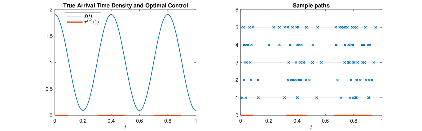
Refer to caption
Figure 4: Optimal on/off system control for the true process and the DRSO.
Example 4.2

Figure 4 shows results for an instance of the on/off system control problem. Suppose that the number of arrivals is Poisson distributed with mean λ\lambda, and given the number of arrivals, the arrival points are i.i.d. with density f⁡(t)f(t), t∈[0,1]t\in[0,1]. For example, f≡1f\equiv 1 corresponds to the Poisson process with rate λ\lambda. The optimization problem based on knowing the process is max⁡∫x−1​(1)x⁡[−c+λ​f​(t)]​𝑑t\max_{x}\int_{x^{-1}(1)}[-c+\lambda f(t)]dt, with optimal control x∗(t)=𝟙{λf(t)>c}x^{\ast}(t)=\mathds{1}_{\{\lambda f(t)>c\}}.

Let f⁡(t)=k⁡[a+sin⁡(w​t+s)]f(t)=k[a+\sin(wt+s)], with a>1a>1 and k=1/[a+(cos⁡(s)−cos⁡(w+s))/w]k=1/[a+(\cos(s)-\cos(w+s))/w]. Particularly, let w=5​πw=5\pi, s=π/2s=\pi/2, a=1.1a=1.1, and c=λ=20c=\lambda=20. Thus x∗−1​(1)=[0,0.1]∪[0.3,0.5]∪[0.7,0.9]{x^{\ast}}^{-1}(1)=[0,0.1]\cup[0.3,0.5]\cup[0.7,0.9]. The left of Figure 4 shows f⁡(t)f(t) and x∗x^{\ast}. Suppose we have N=5N=5 sample paths ξ^1,…,ξ^5\widehat{\xi}^{1},\ldots,\widehat{\xi}^{5}, each of which contains Mi∼P​o​i​s​s​o​n​(λ)M_{i}\sim Poisson(\lambda) i.i.d. arrival points. The right of Figure 4 shows 55 sample paths and the resulting DRSO solution. Even with a relatively small number of sample paths, the two controls are close to each other, and the DRSO provides not only a sensible solution (unlike the approach of optimizing the expected profit with respect to the empirical distribution), but even a good solution for the true process control problem.

4.2 Intensity Estimation for Non-homogeneous Poisson Processes

Consider the problem of estimating the intensity function a⁡(t)a(t) of a non-homogeneous Poisson process A⁡(t)A(t) on [0,T][0,T] using the maximum likelihood method. Given NN i.i.d. sample paths ξ^i=∑m=1Miδη^mi\widehat{\xi}^{i}=\sum_{m=1}^{M_{i}}\delta_{\widehat{\eta}^{i}_{m}}, i=1,…,Ni=1,\ldots,N, the log-likelihood function (see, e.g. Daley and Vere-Jones [18]) is written as

ℒ(a)=−∫0Ta(t)dt+1N∑i=1N∑m=1Miln(a(η^mi)).\mathscr{L}(a)\ \ =\ \ -\int_{0}^{T}a(t)\,dt+\frac{1}{N}\sum_{i=1}^{N}\sum_{m=1}^{M_{i}}\ln\big(a(\widehat{\eta}^{i}_{m})\big).

A common practice is to partition the time horizon [0,T][0,T] into several intervals, and assume that a⁡(t)a(t) is piecewise constant with constant value on each of the chosen intervals. Then the maximum likelihood estimator reduces to the average arrival rate on each interval. Such an approach suffers from the drawback that the estimator is sensitive to the partition of the time horizon into intervals. If the partition is very coarse, then the estimator remains constant during long intervals, and fails to capture time-varying arrival rates over shorter time periods. On the other hand, if the partition is very fine, then many intervals have zero observations, and the estimator varies too erratically over short intervals of time. A DRSO formulation with 𝔐\mathfrak{M} chosen to be the KL-divergence ball 𝔐ϕK​L\mathfrak{M}_{\phi_{KL}} has a similar problem, since the resulting estimator vanishes on intervals with no observations.

Consider the DRSO formulation with Wasserstein distance

mina⁡(t), 0≤t≤T{vθ(a):=∫0Ta(t)dt+maxμ∈𝔐𝔼η∼μ[−∫0Tln(a(t))η(dt)]},\min_{a(t),\;0\leq t\leq T}\ \left\{v_{\theta}(a)\ \vcentcolon=\ \int_{0}^{T}a(t)\,dt+\max_{\mu\in\mathfrak{M}}\;\mathbb{E}_{\eta\sim\mu}\left[-\int_{0}^{T}\ln\big(a(t)\big)\,\eta(dt)\right]\right\}, (40)

where 𝔐\mathfrak{M} is the Wasserstein ball centered at the empirical process. To facilitate further analysis, we choose dd defined in (35) as the distance between two counting measures. Our strong duality results imply that the dual reformulation of (40) is given by

mina⁡(t)λ≥0⁡{∫0Ta⁡(t)​𝑑t+λ​θ+1N​∑i=1N∑m=1Misupη∈[0,T]{−ln⁡(a⁡(ξ))−λ​|η−η^mi|}}.\min_{\begin{subarray}{c}a(t)\\ \lambda\geq 0\end{subarray}}\ \left\{\int_{0}^{T}a(t)dt+\lambda\theta+\frac{1}{N}\sum_{i=1}^{N}\sum_{m=1}^{M_{i}}\sup_{\eta\in[0,T]}\Big\{-\ln\big(a(\xi)\big)-\lambda|\eta-\widehat{\eta}^{i}_{m}|\Big\}\right\}.

Next we present numerical results for underlying true intensity functions given by a⁡(t)=0.2+0.2​ta(t)=0.2+0.2t and a⁡(t)=1+sin⁡(π​t)a(t)=1+\sin(\pi t), t∈[0,10]t\in[0,10]. The sample size (number of sample paths) is N=20N=20. For both the maximum likelihood estimator and the DRSO estimator we optimized over piecewise constant a⁡(t)a(t) with number of pieces in {20,50,100}\{20,50,100\}. The Wasserstein radius θ\theta was chosen via a cross-validation method, in which half of the sample paths were used for estimating aθ∈\argmina​vθ​(a)a_{\theta}\in\argmin_{a}v_{\theta}(a) for each value of θ\theta, and the other half of the sample paths were used for selecting the value of θ∈\argmaxθ​ℒ​(aθ)\theta\in\argmax_{\theta}\mathscr{L}(a_{\theta}) with the largest log-likelihood. The estimation results for both the maximum likelihood estimator (MLE) and the Wasserstein DRSO estimator are shown in Figure 5. Table 1 shows the L2L^{2} distances between the estimated intensity functions and the true intensity functions. The Wasserstein DRSO estimator has superior performance in all cases. Also, the performance of the DRSO estimator is less sensitive to the fineness of the partition for the piecewise constant function than the performance of the maximum likelihood estimator — in these results the performance of the maximum likelihood estimator behaves poorly when the number of pieces is large.

Refer to caption
Refer to caption
Refer to caption
Refer to caption
Refer to caption
Refer to caption
Figure 5: Estimated intensity functions using Wasserstein DRSO and MLE
Table 1: L2L^{2} distances between the true intensity functions and the estimated intensity functions of Wasserstein DRSO and MLE
0.2+0.2​t0.2+0.2t 1+sin⁡(π​t)1+\sin(\pi t)
Pieces 20 50 100 20 50 100
Wasserstein 0.854 0.893 0.544 2.008 2.157 2.087
MLE 1.510 6.536 11.906 6.160 6.591 11.766

4.3 Worst-case Value-at-Risk

Value-at-risk is a popular risk measure in finance. Given a real-valued random variable ZZ that represents losses with measure ν\nu that has a positive density on an interval, and α∈(0,1)\alpha\in(0,1), the value-at-risk VaRαν​[Z]\mathrm{VaR}^{\nu}_{\alpha}[Z] of ZZ is defined by

VaRαν[Z]:=inf{t:ℙν{Z<t}> 1−α}.\mathrm{VaR}^{\nu}_{\alpha}[Z]\ \ \vcentcolon=\ \ \inf\left\{t\;:\;\mathbb{P}_{\nu}\{Z<t\}\,>\,1-\alpha\right\}.

In the spirit of El Ghaoui et al. [21], we consider the following worst-case VaR\mathrm{VaR} problem. Consider a portfolio consisting of KK assets with allocation weights w:=(w1,…,wK)≥0w\vcentcolon=(w_{1},\ldots,w_{K})\geq 0 such that ∑k=1Kwk=1\sum_{k=1}^{K}w_{k}=1. Let ξk\xi_{k} denote the (random) return of asset kk, k=1,…,Kk=1,\ldots,K. Assume that (Ξ,d)=(ℝK,∥⋅∥)(\Xi,d)=(\mathbb{R}^{K},\|\cdot\|). The worst-case VaR\mathrm{VaR} with respect to the set of probability distributions 𝔐\mathfrak{M} is defined as

VaRα𝔐(w):=supμ∈𝔐VaRαμ[−w⊤ξ]=min{q:infμ∈𝔐ℙμ{−w⊤ξ<q}> 1−α}.\mathrm{VaR}^{\mathfrak{M}}_{\alpha}(w)\ \ \vcentcolon=\ \ \sup_{\mu\in\mathfrak{M}}\mathrm{VaR}^{\mu}_{\alpha}[-w^{\top}\xi]\ \ =\ \ \min\left\{q\;:\;\inf_{\mu\in\mathfrak{M}}\mathbb{P}_{\mu}\{-w^{\top}\xi<q\}\,>\,1-\alpha\right\}.

Given ww and qq, let C:={ξ:−w⊤​ξ<q}C\vcentcolon=\{\xi\,:\,-w^{\top}\xi<q\}. Then infμ∈𝔐ℙμ{−w⊤ξ<q}=infμ∈𝔐𝔼μ[𝟙C(ξ)]=minμ∈𝔐μ(C)\inf_{\mu\in\mathfrak{M}}\mathbb{P}_{\mu}\{-w^{\top}\xi<q\}=\inf_{\mu\in\mathfrak{M}}\mathbb{E}_{\mu}[\mathds{1}_{C}(\xi)]\ \ =\ \ \min_{\mu\in\mathfrak{M}}\mu(C), similar to the uncertainty quantification problem (31) considered in Example 3.29. Using the rationale developed there, we obtain the following result.

Proposition 4.3

Suppose that ν\nu has a positive density on (Ξ,d)=(ℝK,∥⋅∥)(\Xi,d)=(\mathbb{R}^{K},\|\cdot\|), α∈(0,1)\alpha\in(0,1), and θ>0\theta>0. Let ww be given, and let νw​{(−∞,s)}:=ν⁡{ξ:−w⊤​ξ<s}\nu_{w}\{(-\infty,s)\}\vcentcolon=\nu\{\xi\,:\,-w^{\top}\xi<s\} for all s∈ℝs\in\mathbb{R}. Then, VaRα𝔐​(w)\mathrm{VaR}^{\mathfrak{M}}_{\alpha}(w) equals the unique solution qq of the following equation:

∫VaRαν​[−w⊤​ξ]q(q−s)p​νw​(𝑑s)=θp​‖w‖∗p.\int_{\mathrm{VaR}^{\nu}_{\alpha}[-w^{\top}\xi]}^{q}(q-s)^{p}\nu_{w}(ds)\ \ =\ \ \theta^{p}\|w\|_{\ast}^{p}.
Refer to caption
Figure 6: Worst-case VaR. When −w⊤​ξ-w^{\top}\xi has a continuous cumulative distribution function, and p=1p=1, then VaRα𝔐\mathrm{VaR}_{\alpha}^{\mathfrak{M}} is equal to the value of qq such that the area of the shaded region is equal to θ​‖w‖∗\theta\|w\|_{\ast}.
Example 4.4 (Worst-case VaR\mathrm{VaR} with Gaussian nominal distribution)

Suppose that ν=N⁡(μ¯,Σ)\nu=N(\bar{\mu},\Sigma) and p=1p=1. It follows that −w⊤​ξ∼N⁡(−w⊤​μ¯,w⊤​Σ​w)-w^{\top}\xi\sim N(-w^{\top}\bar{\mu},w^{\top}\Sigma w) and VaRαν​[−w⊤​ξ]=−w⊤​μ¯+w⊤​Σ​w​Φ−1​(1−α)\mathrm{VaR}^{\nu}_{\alpha}[-w^{\top}\xi]=-w^{\top}\bar{\mu}+\sqrt{w^{\top}\Sigma w}\Phi^{-1}(1-\alpha), where Φ=N⁡(0,1)\Phi=N(0,1). By Proposition 4.3, VaRα𝔐​(−w⊤​ξ)\mathrm{VaR}_{\alpha}^{\mathfrak{M}}(-w^{\top}\xi) is the value of qq such that (see Figure 6)

f⁡(q):=12​π​w⊤​Σ​w​∫VaRαν​[−w⊤​ξ]q(q−y)​e−(y+w⊤​μ¯)22​w⊤​Σ​w​𝑑y=θ​‖w‖∗.f(q)\ \ \vcentcolon=\ \ \frac{1}{\sqrt{2\pi w^{\top}\Sigma w}}\int_{\mathrm{VaR}^{\nu}_{\alpha}[-w^{\top}\xi]}^{q}(q-y)\,e^{-\frac{(y+w^{\top}\bar{\mu})^{2}}{2w^{\top}\Sigma w}}\,dy\ \ =\ \ \theta\|w\|_{\ast}. (41)

Since f⁡(q)f(q) is increasing and continuous, (41) can be solved efficiently via a one-dimensional search algorithm.

Proposition 4.3 indicates that finding the worst-case VaR\mathrm{VaR} is tractable. It should also be noted that finding the best allocation weight, i.e., optimizing over ww, still may be hard, since the VaR\mathrm{VaR} constraint is essentially a chance constraint.

5 Discussions

In this section, we discuss some of the advantages of using the Wasserstein ambiguity set. In Section 5.1, we compare DRSO with the Wasserstein ambiguity set to DRSO with ϕ\phi-divergence ambiguity sets for the newsvendor problem. In Section 5.2, we illustrate how the close connection between DRSO and robust optimization (Corollary 3.32(iii)) can be used to solve DRSO problems.

5.1 Newsvendor Problem: Comparison with ϕ\phi-divergence

In this section, we consider distributionally robust newsvendor problems, and compare results obtained with the Wasserstein ambiguity set and results obtained with ϕ\phi-divergence ambiguity sets. In the newsvendor problem, the decision maker chooses the initial inventory level before the unknown demand is observed, facing both overage and underage costs. If the demand distribution μ\mu is known, the problem can be formulated as

minx≥0⁡𝔼μ​[h​[x−ξ]++b​[ξ−x]+],\min_{x\geq 0}\ \mathbb{E}_{\mu}[h[x-\xi]^{+}+b[\xi-x]^{+}],

where xx denotes the chosen initial inventory level, ξ\xi denotes the random demand, and hh, bb represent respectively the overage and underage costs per unit. Assume that h,b>0h,b>0, and μ\mu is supported on {0,1,…,B}\{0,1,\ldots,B\} for some positive integer BB. Consider the usual metric d⁡(i,j)=|i−j|d(i,j)=|i-j| on {0,1,…,B}\{0,1,\ldots,B\}.

Usually the demand distribution μ\mu is not known. Then the decision maker may want to consider the DRSO problem

min⁡supμ∈ΔBx≥0⁡{𝔼μ​[h​[x−ξ]++b​[ξ−x]+]:Wp​(μ,ν)≤θ}.\min_{x\geq 0}\ \sup_{\mu\in\Delta_{B}}\left\{\mathbb{E}_{\mu}[h[x-\xi]^{+}+b[\xi-x]^{+}]\;:\;W_{p}(\mu,\nu)\leq\theta\right\}.

Using Corollary 3.32, we obtain a convex optimization reformulation

minx≥0,λ≥0,y:=(y0,…,yB){λθp+∑i=0Bνiyi:yi≥max{h(x−j),b(j−x)}−λ|i−j|p,∀ 0≤i,j≤B}.\min_{x\geq 0,\lambda\geq 0,y\vcentcolon=(y_{0},\ldots,y_{B})}\left\{\lambda\theta^{p}+\sum_{i=0}^{B}\nu_{i}y_{i}\;:\;y_{i}\geq\max\big\{h(x-j),b(j-x)\big\}-\lambda|i-j|^{p},\;\forall\;0\leq i,j\leq B\right\}.
Table 2: Examples of ϕ\phi-divergence
Divergence Kullback-Leibler Burg entropy χ2\chi^{2}-distance Modified χ2\chi^{2} Hellinger Total Variation
ϕ\phi ϕk​l\phi_{kl} ϕb\phi_{b} ϕχ2\phi_{\chi^{2}} ϕm​χ2\phi_{m\chi^{2}} ϕh\phi_{h} ϕt​v\phi_{tv}
ϕ⁡(t),t≥0\phi(t),t\geq 0 t​log⁡tt\log t −log⁡t-\log t 1t​(t−1)2\frac{1}{t}(t-1)^{2} (t−1)2(t-1)^{2} (t−1)2(\sqrt{t}-1)^{2} |t−1||t-1|
Iϕ​(μ,ν)I_{\phi}(\mu,\nu) ∑pj​log⁡(pjqj)\sum p_{j}\log\left(\frac{p_{j}}{q_{j}}\right) ∑qj​log⁡(qjpj)\sum q_{j}\log\left(\frac{q_{j}}{p_{j}}\right) ∑(pj−qj)2pj\sum\frac{(p_{j}-q_{j})^{2}}{p_{j}} ∑(pj−qj)2qj\sum\frac{(p_{j}-q_{j})^{2}}{q_{j}} ∑(pj−qj)2\sum(\sqrt{p_{j}}-\sqrt{q_{j}})^{2} ∑|pj−qj|\sum|p_{j}-q_{j}|

One may also consider ϕ\phi-divergence ambiguity sets (Table 2 shows some common ϕ\phi-divergences). As mentioned in Section 1, the worst-case distribution in a ϕ\phi-divergence ambiguity set may be problematic. For example, when limt→∞ϕ⁡(t)/t=∞\lim_{t\to\infty}\phi(t)/t=\infty, such as ϕk​l\phi_{kl} and ϕm​χ2\phi_{m\chi^{2}}, the ϕ\phi-divergence ambiguity set fails to include many relevant distributions. Specifically, since 0​ϕ​(pj/0):=pj​limt→∞ϕ⁡(t)/t=∞0\phi(p_{j}/0)\vcentcolon=p_{j}\lim_{t\to\infty}\phi(t)/t=\infty for all pj>0p_{j}>0, the ϕk​l\phi_{kl}- and ϕm​χ2\phi_{m\chi^{2}}-divergence ambiguity sets do not include any distribution which is not absolutely continuous with respect to the nominal distribution ν\nu.

When limt→∞ϕ⁡(t)/t<∞\lim_{t\to\infty}\phi(t)/t<\infty, such as ϕb\phi_{b}, ϕχ2\phi_{\chi^{2}}, ϕh\phi_{h}, and ϕt​v\phi_{tv}, the situation is also bad. Let I0:={j∈{0,…,B}:qj>0}I_{0}\vcentcolon=\{j\in\{0,\ldots,B\}\,:\,q_{j}>0\}. Assume that Ψ⁡(ξj)\Psi(\xi^{j}) are different from each other, so that jM∈\argmaxj∈{0,…,B}​{Ψ⁡(ξj):qj=0}j_{M}\in\argmax_{j\in\{0,\ldots,B\}}\{\Psi(\xi^{j})\,:\,q_{j}=0\} is unique. Then according to Ben-Tal et al. [7] and Bayraksan and Love [6], the worst-case distribution p∗p^{\ast} satisfies

pj∗qj\displaystyle\frac{p_{j}^{\ast}}{q_{j}} ∈\displaystyle\ \ \in\ \ ∂ϕ∗​(Ψ⁡(ξj)−β∗λ∗),∀i∈I0,\displaystyle\partial\phi^{\ast}\left(\frac{\Psi(\xi^{j})-\beta^{\ast}}{\lambda^{\ast}}\right),\qquad\forall\ i\in I_{0}, (42a)
pj∗\displaystyle p_{j}^{\ast} =\displaystyle\ \ =\ \ 0,∀j∉I0∪{jM},\displaystyle 0,\qquad\forall\ j\notin I_{0}\cup\{j_{M}\}, (42b)
pjM∗\displaystyle p_{j_{M}}^{\ast} =\displaystyle\ \ =\ \ {1−∑i∈I0pj∗ if ​β∗=Ψ⁡(ξjM)−λ∗​limt→∞ϕ⁡(t)/t,0 if ​β∗>Ψ⁡(ξjM)−λ∗​limt→∞ϕ⁡(t)/t,\displaystyle\left\{\begin{array}[]{ll}1-\sum_{i\in I_{0}}p_{j}^{\ast}&\textrm{ if }\beta^{\ast}=\Psi(\xi^{j_{M}})-\lambda^{\ast}\lim_{t\to\infty}\phi(t)/t,\\ 0&\textrm{ if }\beta^{\ast}>\Psi(\xi^{j_{M}})-\lambda^{\ast}\lim_{t\to\infty}\phi(t)/t,\end{array}\right.

for some λ∗≥0\lambda^{\ast}\geq 0 and β∗≥Ψ⁡(ξjM)−λ∗​limt→∞ϕ⁡(t)/t\beta^{\ast}\geq\Psi(\xi^{j_{M}})-\lambda^{\ast}\lim_{t\to\infty}\phi(t)/t, where ϕ∗\phi^{\ast} denotes the convex conjugate function of ϕ\phi. According to (42b), the support of the worst-case distribution and that of the nominal distribution can differ by at most one point ξjM\xi^{j_{M}}. According to (42), the probability mass pjM∗p^{\ast}_{j_{M}} is moved away from scenarios in I0I_{0} to the worst scenario ξjM\xi^{j_{M}}. Note that in many applications where the support of ξ\xi is unknown, the choice of the underlying space Ξ\Xi (such as {0,1,…,B}\{0,1,\ldots,B\}) may be somewhat arbitrary, and therefore the worst scenario ξjM\xi^{j_{M}} (such as 00 or BB) may be arbitrary. Hence the worst-case behavior is too sensitive to arbitrary choices in the specification of Ξ\Xi.

We present numerical examples of which the setup is similar to that in Wang et al. [52] and Ben-Tal et al. [7]. Let b=h=1b=h=1, B=100B=100, and N∈{50,500}N\in\{50,500\} representing small and large datasets. Random data are generated from Binomial(100,0.5)(100,0.5) and Geometric(0.1)(0.1) truncated on [0,100][0,100]. We estimate the radius of the ambiguity set such that it covers the underlying distribution with probability greater than 0.950.95 (see Appendix C).

(a) Binomial(100,0.5)(100,0.5), N=500N=500
(b) Binomial(100,0.5)(100,0.5), N=50N=50
(c) truncated Geometric(0.1)(0.1), N=500N=500
(d) truncated Geometric(0.1)(0.1), N=50N=50
Figure 7: Histograms of worst-case distributions resulting from Wasserstein distance and Burg entropy

When the underlying distribution is Binomial, the symmetry of the Binomial distribution and b=h=1b=h=1 implies that the optimal initial inventory level is close to 5050. Intuitively, the corresponding worst-case distribution should make provision for both the possibility of high demand and the possibility of low demand. This intuition is consistent with the worst-case distributions in the Wasserstein ambiguity set, shown by the solid curves in Figures (7a)–(7b). The tails of these worst-case distributions are heavy on both the high side and the low side, and are quite smooth and reasonable for both small and large datasets. In contrast, if Burg entropy is used to define the ambiguity set, then the worst-case distributions have disconnected support, as shown by the dashed curves in Figures (7a)–(7b). There is a large spike on the boundary B=100B=100, displaying the “popping” behavior mentioned in Bayraksan and Love [6]. Especially when the dataset is small, the worst-case spike is huge, which makes the solution too conservative.

When the underlying distribution is Geometric, the worst-case distributions in the Wasserstein ambiguity set make provision for both the possibility of high demand and the possibility of low demand with fairly smooth variation of probability in between, as shown by solid curves in Figures (7c)–(7d). As before, if Burg entropy is used, then the tail has unrealistic spikes on the boundary, and thus the worst-case distribution is very sensitive to the somewhat arbitrary choice of truncation value BB. In these examples the Wasserstein ambiguity set seems to yield a more reasonable worst-case distribution.

5.2 Two-stage DRSO: Connection with Robust Optimization

In Corollary 3.19(iii) we established the close connection between the DRSO problem and robust optimization. More specifically, we showed that every DRSO problem can be approximated with high accuracy by robust optimization problems, which facilitates practical application of DRSO problems. To illustrate this point, in this section we show the tractability of two-stage linear DRSO problems.

Consider the two-stage distributionally robust stochastic optimization problem

minx∈X⁡c⊤​x+supμ∈𝔐𝔼μ​[Ψ⁡(x,ξ)],\min_{x\in X}c^{\top}x+\sup_{\mu\in\mathfrak{M}}\mathbb{E}_{\mu}[\Psi(x,\xi)], (43)

where Ψ⁡(x,ξ)\Psi(x,\xi) is the optimal objective value of the second-stage problem

Ψ⁡(x,ξ):=miny∈ℝm⁡{q​(ξ)⊤​y:T⁡(ξ)​x+W⁡(ξ)​y≤h⁡(ξ)}\Psi(x,\xi)\ \ \vcentcolon=\ \ \min_{y\in\mathbb{R}^{m}}\left\{q(\xi)^{\top}y\;:\;T(\xi)x+W(\xi)y\leq h(\xi)\right\}

and

q⁡(ξ)=q0+∑l=1sξl​ql,T⁡(ξ)=T0+∑l=1sξl​Tl,W⁡(ξ)=W0+∑l=1sξl​Wl,h⁡(ξ)=h0+∑l=1sξl​hl.q(\xi)\ =\ q^{0}+\sum_{l=1}^{s}\xi_{l}q^{l},\ \ T(\xi)\ =\ T^{0}+\sum_{l=1}^{s}\xi_{l}T^{l},\ \ W(\xi)\ =\ W^{0}+\sum_{l=1}^{s}\xi_{l}W^{l},\ \ h(\xi)\ =\ h^{0}+\sum_{l=1}^{s}\xi_{l}h^{l}.

Assume that p=2p=2 and Ξ=ℝs\Xi=\mathbb{R}^{s} with Euclidean distance dd. In general, the two-stage problem (43) is NP-hard (see Section 3.3.2 in [31]). However, with tools from robust optimization, we are able to obtain a tractable approximation of (43). Let 𝔐1:={(ξ1,…,ξN)∈ΞN:1N​∑i=1N‖ξi−ξ^i‖22≤θ2}\mathfrak{M}_{1}\vcentcolon=\{(\xi^{1},\ldots,\xi^{N})\in\Xi^{N}\,:\,\frac{1}{N}\sum_{i=1}^{N}\|\xi^{i}-\widehat{\xi}^{i}\|_{2}^{2}\leq\theta^{2}\}. Using Corollary 3.19(iii) with K=1K=1, we obtain an adjustable robust optimization approximation

minx∈X⁡{c⊤​x+sup(ξi)i=1N∈𝔐11N​∑i=1NΨ⁡(x,ξi)}\displaystyle\min_{x\in X}\left\{c^{\top}x+\sup_{(\xi^{i})_{i=1}^{N}\in\mathfrak{M}_{1}}\frac{1}{N}\sum_{i=1}^{N}\Psi(x,\xi^{i})\right\} (44)
=\displaystyle= minx∈X,t∈ℝ,y:Ξ↦ℝm{t:t≥c⊤x+1N∑i=1Nq(ξi)⊤y(ξi),∀(ξi)i=1N∈𝔐1,T⁡(ξ)​x+W⁡(ξ)​y​(ξ)≤h⁡(ξ),∀ξ∈⋃i=1N{ξ′∈Ξ:‖ξ′−ξ^i‖2≤θ​N}},\displaystyle\min_{\begin{subarray}{c}x\in X,t\in\mathbb{R},\\ y:\Xi\mapsto\mathbb{R}^{m}\end{subarray}}\left\{t\;:\;\begin{array}[]{l}t\ \geq\ c^{\top}x+\frac{1}{N}\sum_{i=1}^{N}q(\xi^{i})^{\top}y(\xi^{i}),\ \forall\ (\xi^{i})_{i=1}^{N}\in\mathfrak{M}_{1},\\ T(\xi)x+W(\xi)y(\xi)\ \leq\ h(\xi),\ \forall\ \xi\in\bigcup_{i=1}^{N}\{\xi^{\prime}\in\Xi\;:\;\|\xi^{\prime}-\widehat{\xi}^{i}\|_{2}\leq\theta\sqrt{N}\}\end{array}\right\},

where the second set of inequalities follows from the fact that T⁡(ξ)​x+W⁡(ξ)​y​(ξ)≤h⁡(ξ)T(\xi)x+W(\xi)y(\xi)\leq h(\xi) should hold for any realization ξ\xi with positive probability for some distribution in 𝔐1\mathfrak{M}_{1}. Although problem (44) in general is still intractable, there has been a substantial literature on different approximations for problem (44). One approach is to consider the affinely adjustable robust counterpart (AARC), as follows. Consider yy that is an affine function of ξ\xi:

y⁡(ξ)=y0+∑l=1sξl​yl,∀ξ∈⋃i=1NBi,y(\xi)\ \ =\ \ y^{0}+\sum_{l=1}^{s}\xi_{l}y^{l},\ \ \forall\ \xi\in\bigcup_{i=1}^{N}B^{i},

for some chosen y0,yl∈ℝmy^{0},y^{l}\in\mathbb{R}^{m}, where Bi:={ξ′∈Ξ:‖ξ′−ξ^i‖2≤θ​N}B^{i}\vcentcolon=\{\xi^{\prime}\in\Xi\,:\,\|\xi^{\prime}-\widehat{\xi}^{i}\|_{2}\leq\theta\sqrt{N}\}. Then the AARC of (44) is

minx∈X,t∈ℝ,yl∈ℝm,l=0,…,s\displaystyle\min_{\begin{subarray}{c}x\in X,t\in\mathbb{R},\\ y^{l}\in\mathbb{R}^{m},l=0,\ldots,s\end{subarray}} {t:c⊤x+1N∑i=1N(q0+∑l=1sξilql)⊤(y0+∑l=1sξilyl)−t≤ 0,∀(ξi)i=1N∈𝔐1,\displaystyle\Bigg\{t\;:\;c^{\top}x+\frac{1}{N}\sum_{i=1}^{N}\left(q^{0}+\sum_{l=1}^{s}\xi^{i}_{l}q^{l}\right)^{\top}\left(y^{0}+\sum_{l=1}^{s}\xi^{i}_{l}y^{l}\right)-t\ \leq\ 0,\ \forall\ (\xi^{i})_{i=1}^{N}\in\mathfrak{M}_{1}, (45)
(T0+∑l=1sξlTl)x+(W0+∑l=1sξlWl)(y0+∑l=1sξlyl)−(h0+∑l=1sξlhl)≤ 0,∀ξ∈⋃i=1NBi}.\displaystyle\left(T^{0}+\sum_{l=1}^{s}\xi_{l}T^{l}\right)x+\left(W^{0}+\sum_{l=1}^{s}\xi_{l}W^{l}\right)\left(y^{0}+\sum_{l=1}^{s}\xi_{l}y^{l}\right)-\left(h^{0}+\sum_{l=1}^{s}\xi_{l}h^{l}\right)\ \leq\ 0,\ \forall\ \xi\in\bigcup_{i=1}^{N}B^{i}\Bigg\}.

Set ζi​l:=ξli−ξ^li\zeta_{il}\vcentcolon=\xi^{i}_{l}-\widehat{\xi}^{i}_{l} for i=1,…,Ni=1,\ldots,N and l=1,…,sl=1,\ldots,s. Note that (ξ1,…,ξN)∈𝔐1(\xi^{1},\ldots,\xi^{N})\in\mathfrak{M}_{1} if and only if

ζ:=(ζi​l)i,l∈𝒰:={(ζi​l′)i,l:∑i=1N∑l=1sζ′i​l2≤N​θ2}.\zeta\ \ \vcentcolon=\ \ (\zeta_{il})_{i,l}\ \ \in\ \ \mathcal{U}\ \ \vcentcolon=\ \ \{(\zeta^{\prime}_{il})_{i,l}\;:\;\sum_{i=1}^{N}\sum_{l=1}^{s}{\zeta^{\prime}}_{il}^{2}\leq N\theta^{2}\}.

Set z:=(x,t,{yl}l=0s)z\vcentcolon=\left(x,t,\{y^{l}\}_{l=0}^{s}\right), and let

α0​(z)\displaystyle\alpha_{0}(z)\ \ :=−[c⊤x+1N∑i=1N(q0+∑l=1sξ^liql)⊤(y0+∑l=1sξ^liyl)−t],\displaystyle\vcentcolon=\ \ -\left[c^{\top}x+\frac{1}{N}\sum_{i=1}^{N}\left(q^{0}+\sum_{l=1}^{s}\widehat{\xi}^{i}_{l}q^{l}\right)^{\top}\left(y^{0}+\sum_{l=1}^{s}\widehat{\xi}^{i}_{l}y^{l}\right)-t\right],
β0i​l​(z)\displaystyle\beta_{0}^{il}(z)\ \ :=−[(q0+∑l′=1sξ^l′i​ql′)⊤​yl+ql⊤​(y0+∑l′=1sξ^l′i​yl′)]2​N,∀i=1,…,N,l=1,…,s.\displaystyle\vcentcolon=\ \ -\frac{\left[\left(q^{0}+\sum_{l^{\prime}=1}^{s}\widehat{\xi}^{i}_{l^{\prime}}q^{l^{\prime}}\right)^{\top}y^{l}+{q^{l}}^{\top}\left(y^{0}+\sum_{l^{\prime}=1}^{s}\widehat{\xi}^{i}_{l^{\prime}}y^{l^{\prime}}\right)\right]}{2N},\qquad\forall\ i=1,\ldots,N,\ l=1,\ldots,s.
Γ0(l,l′)​(z)\displaystyle\Gamma_{0}^{(l,l^{\prime})}(z)\ \ :=−ql⊤​yl′+ql′⊤​yl2​N,∀l,l′=1,…,s.\displaystyle\vcentcolon=\ \ -\frac{{q^{l}}^{\top}{y^{l^{\prime}}}+{q^{l^{\prime}}}^{\top}{y^{l}}}{2N},\qquad\forall\ l,l^{\prime}=1,\ldots,s.

Then the first set of constraints in (45) is equivalent to

α0​(z)+2​∑i=1N∑l=1sβ0i​l​(z)​ζi​l+∑i=1N∑l=1s∑l′=1sΓ0(l,l′)​(z)​ζi​l​ζi​l′≥ 0,∀ζ∈𝒰.\alpha_{0}(z)+2\sum_{i=1}^{N}\sum_{l=1}^{s}\beta_{0}^{il}(z)\zeta_{il}+\sum_{i=1}^{N}\sum_{l=1}^{s}\sum_{l^{\prime}=1}^{s}\Gamma_{0}^{(l,l^{\prime})}(z)\zeta_{il}\zeta_{il^{\prime}}\ \ \geq\ \ 0,\qquad\forall\ \zeta\in\mathcal{U}. (46)

It follows from Theorem 4.2 in Ben-Tal et al. [8] that (46) holds if and only if there exists λ0≥0\lambda_{0}\geq 0 such that

(α0​(z)−λ0)​v2+2​v​∑i=1N∑l=1sβ0i​l​(z)​wi​l+∑i=1N∑l=1s∑l′=1sΓ0(l,l′)​(z)​wi​l​wi​l′+λ0N​θ2​∑i=1N∑l=1swi​l2≥ 0,\displaystyle(\alpha_{0}(z)-\lambda_{0})v^{2}+2v\sum_{i=1}^{N}\sum_{l=1}^{s}\beta_{0}^{il}(z)w_{il}+\sum_{i=1}^{N}\sum_{l=1}^{s}\sum_{l^{\prime}=1}^{s}\Gamma_{0}^{(l,l^{\prime})}(z)w_{il}w_{il^{\prime}}+\frac{\lambda_{0}}{N\theta^{2}}\sum_{i=1}^{N}\sum_{l=1}^{s}w_{il}^{2}\ \ \geq\ \ 0,
∀v∈ℝ,wi​l∈ℝ,i=1,…,N,l=1,…,s.\displaystyle\forall\ v\in\mathbb{R},\ w_{il}\in\mathbb{R},\ i=1,\ldots,N,\ l=1,\ldots,s.

In matrix form,

∃λ0≥0:(Γ0​(z)⊗IN+λ0N​θ2​Is​Nvec​(β0​(z))vec​(β0​(z))⊤α0​(z)−λ0)⪰ 0,\exists\lambda_{0}\geq 0\ :\ \left(\begin{array}[]{cc}\Gamma_{0}(z)\otimes I_{N}+\frac{\lambda_{0}}{N\theta^{2}}I_{sN}&\ \ \mathrm{vec}(\beta_{0}(z))\\ \mathrm{vec}(\beta_{0}(z))^{\top}&\ \ \alpha_{0}(z)-\lambda_{0}\end{array}\right)\ \ \succeq\ \ 0, (47)

where INI_{N} (resp. Is​NI_{sN}) is the N×NN\times N (resp. s​N×s​NsN\times sN) identity matrix, ⊗\otimes is the Kronecker product of matrices, vec⁡(β0)\mathrm{vec}(\beta_{0}) is the vectorization of matrix β0​(z)\beta_{0}(z), and Γ0​(z)\Gamma_{0}(z) is a matrix whose (l,l′)(l,l^{\prime})-element equal to Γ0(l,l′)​(z)\Gamma_{0}^{(l,l^{\prime})}(z).

Next we reformulate the second set of constraints in (45). Let TjlT_{j}^{l} and WjlW_{j}^{l} denote row jj of TlT^{l} and WlW^{l}, respectively, j=1,…,Jj=1,\ldots,J. For all i=1,…,Ni=1,\ldots,N, j=1,…,Jj=1,\ldots,J, and l,l′=1,…,sl,l^{\prime}=1,\ldots,s, set

αi​j​(z)\displaystyle\alpha_{ij}(z)\ \ :=−[(Tj0+∑l=1sξ^liTjl)x+(Wj0+∑l=1sξ^liWjl)(y0+∑l=1sξ^liyl)−(hj0+∑l=1sξ^lihjl)],\displaystyle\vcentcolon=\ \ -\left[\left(T_{j}^{0}+\sum_{l=1}^{s}\widehat{\xi}^{i}_{l}T_{j}^{l}\right)x+\left(W_{j}^{0}+\sum_{l=1}^{s}\widehat{\xi}^{i}_{l}W_{j}^{l}\right)\left(y^{0}+\sum_{l=1}^{s}\widehat{\xi}^{i}_{l}y^{l}\right)-\left(h_{j}^{0}+\sum_{l=1}^{s}\widehat{\xi}^{i}_{l}h_{j}^{l}\right)\right],
βi​jl​(z)\displaystyle\beta_{ij}^{l}(z)\ \ :=−[Tjl​x+(Wj0+∑l=1sξ^li​Wjl)​yl+Wjl​(y0+∑l=1sξ^li​yl)−hjl]2,\displaystyle\vcentcolon=\ \ -\frac{\left[T_{j}^{l}x+\left(W_{j}^{0}+\sum_{l=1}^{s}\widehat{\xi}^{i}_{l}W_{j}^{l}\right)y^{l}+W_{j}^{l}\left(y^{0}+\sum_{l=1}^{s}\widehat{\xi}^{i}_{l}y^{l}\right)-h_{j}^{l}\right]}{2},
Γj(l,l′)​(z)\displaystyle\Gamma_{j}^{(l,l^{\prime})}(z)\ \ :=−Wjl​yl′+Wjl′​yl2.\displaystyle\vcentcolon=\ \ -\frac{W_{j}^{l}y^{l^{\prime}}+W_{j}^{l^{\prime}}y^{l}}{2}.

Let ηi:=ξ−ξ^i\eta^{i}\vcentcolon=\xi-\widehat{\xi}^{i}, βi​j​(z):=(βi​jl​(z))l\beta_{ij}(z)\vcentcolon=(\beta_{ij}^{l}(z))_{l}, and Γj​(z):=(Γj(l,l′)​(z))l,l′\Gamma_{j}(z)\vcentcolon=(\Gamma_{j}^{(l,l^{\prime})}(z))_{l,l^{\prime}}. Then the second set of constraints in (45) is equivalent to

αi​j(z)+2βi​j(z)⊤ηi+ηi⊤Γj(z)ηi≥ 0,∀ηi∈{η′∈ℝs:∥η′∥2≤θN},i=1,…,N,j=1,…,J.\alpha_{ij}(z)+2\beta_{ij}(z)^{\top}\eta^{i}+{\eta^{i}}^{\top}\Gamma_{j}(z)\eta^{i}\ \ \geq\ \ 0,\qquad\forall\ \eta^{i}\in\{\eta^{\prime}\in\mathbb{R}^{s}\;:\;\|\eta^{\prime}\|_{2}\leq\theta\sqrt{N}\},\ i=1,\ldots,N,\ j=1,\ldots,J.

Again by Theorem 4.2 in Ben-Tal et al. [8] the second set of constraints in (45) is equivalent to

∃λi​j≥0:(Γj​(z)+λi​jN​θ2​Isβi​j​(z)βi​j​(z)⊤αi​j​(z)−λi​j)⪰ 0,∀i=1,…,N,j=1,…,J.\exists\lambda_{ij}\geq 0\ :\ \left(\begin{array}[]{cc}\Gamma_{j}(z)+\frac{\lambda_{ij}}{N\theta^{2}}\;I_{s}&\ \ \beta_{ij}(z)\\ \beta_{ij}(z)^{\top}&\ \ \alpha_{ij}(z)-\lambda_{ij}\end{array}\right)\ \ \succeq\ \ 0,\qquad\forall\ i=1,\ldots,N,\ j=1,\ldots,J. (48)

Combining (47) and (48) we obtain the following result.

Proposition 5.1

An exact semidefinite program reformulation of the AARC of (44) is given by

minx∈X,t∈ℝ,yl∈ℝm,l=0,…,s,λ0,λi​j≥0,i=1,…,N,j=1,…,J{t:(47),(48) holds}.\min_{\begin{subarray}{c}x\in X,t\in\mathbb{R},y^{l}\in\mathbb{R}^{m},l=0,\ldots,s,\\ \lambda_{0},\lambda_{ij}\geq 0,i=1,\ldots,N,j=1,\ldots,J\end{subarray}}\left\{t\ :\ (\ref{eqn:AARC_1stconstr_SDP}),(\ref{eqn:AARC_2ndconstr_SDP})\textrm{ holds}\right\}. (49)

By Corollary 3.19(iii), (44) is a fairly good approximation of the original two-stage DRSO problem (43). Hence, as long as the AARC of (44) is reasonably good, its semidefinite program reformulation (49) provides a good tractable approximation of the two-stage linear DRSO (43).

6 Conclusions

In this paper, we developed a constructive proof method to derive the dual reformulation of distributionally robust stochastic optimization with Wasserstein distance for a general setting. This approach allows us to obtain a precise structural description of the worst-case distribution. It also facilitates a connection between distributionally robust stochastic optimization and robust optimization. We showed how the results can be used to obtain theoretical and computational conclusions for a variety of problems.

Appendix A Proofs for Section 2

Proof A.1

Proof of Lemma 2.5. Let (u0,v0)(u_{0},v_{0}) be any feasible solution for the maximization problem in (2). For any t∈ℝt\in\mathbb{R} and any ξ,ζ∈Ξ\xi,\zeta\in\Xi, let ut​(ξ):=u0​(ξ)+tu_{t}(\xi)\vcentcolon=u_{0}(\xi)+t and vt​(ζ):=v0​(ζ)−tv_{t}(\zeta)\vcentcolon=v_{0}(\zeta)-t. Then it follows that ut​(ξ)+vt​(ζ)≤dp​(ξ,ζ)u_{t}(\xi)+v_{t}(\zeta)\leq d^{p}(\xi,\zeta) for all ξ,ζ∈Ξ\xi,\zeta\in\Xi, and

∫Ξut​(ξ)​μ​(𝑑ξ)+∫Ξvt​(ζ)​ν​(𝑑ζ)=∫Ξu0​(ξ)​μ​(𝑑ξ)+∫Ξv0​(ζ)​ν​(𝑑ζ)+t⁡[μ⁡(Ξ)−ν⁡(Ξ)].\int_{\Xi}u_{t}(\xi)\mu(d\xi)+\int_{\Xi}v_{t}(\zeta)\nu(d\zeta)\ \ =\ \ \int_{\Xi}u_{0}(\xi)\mu(d\xi)+\int_{\Xi}v_{0}(\zeta)\nu(d\zeta)+t[\mu(\Xi)-\nu(\Xi)].

Since μ⁡(Ξ)≠ν⁡(Ξ)\mu(\Xi)\neq\nu(\Xi),

supt∈ℝ{∫Ξut​(ξ)​μ​(𝑑ξ)+∫Ξvt​(ζ)​ν​(𝑑ζ)}=∞,\sup_{t\in\mathbb{R}}\left\{\int_{\Xi}u_{t}(\xi)\mu(d\xi)+\int_{\Xi}v_{t}(\zeta)\nu(d\zeta)\right\}\ \ =\ \ \infty,

and thus Wpp​(μ,ν)=∞W_{p}^{p}(\mu,\nu)=\infty.

Appendix B Proofs for Section 3

B.1 Proofs for Section 3.1

B.1.1 Auxiliary results

Lemma B.1

Consider any p≥1p\geq 1 and any ε>0\varepsilon>0. Then there exists Cp​(ε)≥1C_{p}(\varepsilon)\geq 1 such that

(x+y)p≤(1+ε)​xp+Cp​(ε)​yp(x+y)^{p}\ \ \leq\ \ (1+\varepsilon)x^{p}+C_{p}(\varepsilon)y^{p}

for all x,y≥0x,y\geq 0.

Proof B.2

Proof of Lemma B.1. Note that if x=0x=0, then the inequality holds for any Cp​(ε)≥1C_{p}(\varepsilon)\geq 1. Next we consider the case with x>0x>0, and we let t:=y/xt\vcentcolon=y/x. Let

t0​(ε):=sup{t>0: 1+ε≥(1+t)p}.t_{0}(\varepsilon)\ \ \vcentcolon=\ \ \sup\{t>0\;:\;1+\varepsilon\,\geq\,(1+t)^{p}\}.

Note that t0​(ε)>0t_{0}(\varepsilon)>0. Next let

Cp​(ε):=max⁡{1,supt≥t0​(ε)(1+t)p−1tp−1}.C_{p}(\varepsilon)\ \ \vcentcolon=\ \ \max\left\{1,\ \sup_{t\geq t_{0}(\varepsilon)}\frac{(1+t)^{p-1}}{t^{p-1}}\right\}.

Note that Cp​(ε)<∞C_{p}(\varepsilon)<\infty because limt→∞(1+t)p−1/tp−1=1\lim_{t\to\infty}(1+t)^{p-1}/t^{p-1}=1. Next, consider

f⁡(t):= 1+ε+Cp​(ε)​tp−(1+t)pf(t)\ \ \vcentcolon=\ \ 1+\varepsilon+C_{p}(\varepsilon)t^{p}-(1+t)^{p}

Note that f⁡(t)≥0f(t)\geq 0 for all t∈[0,t0​(ε)]t\in[0,t_{0}(\varepsilon)]. Also, f′​(t)=Cp​(ε)​p​tp−1−p​(1+t)p−1≥0f^{\prime}(t)=C_{p}(\varepsilon)pt^{p-1}-p(1+t)^{p-1}\geq 0 for all t∈[t0​(ε),∞)t\in[t_{0}(\varepsilon),\infty). Therefore f⁡(t)≥0f(t)\geq 0 for all t≥0t\geq 0, which establishes the inequality for x>0x>0. □\square

Lemma B.3

Consider any ζ0∈Ξ\zeta^{0}\in\Xi. Then for any λ>λ1>κ\lambda>\lambda_{1}>\kappa, there exists a constant C>0C>0 such that

λ−λ12​D¯​(λ,ζ)≤Φ⁡(λ,ζ)−Φ⁡(λ1,ζ0)+λ1​C​dp​(ζ,ζ0)\frac{\lambda-\lambda_{1}}{2}\overline{D}(\lambda,\zeta)\ \ \leq\ \ \Phi(\lambda,\zeta)-\Phi(\lambda_{1},\zeta^{0})+\lambda_{1}Cd^{p}(\zeta,\zeta^{0})

for all ζ∈Ξ\zeta\in\Xi.

Proof B.4

Proof of Lemma B.3. It follows from Lemma B.1 with ε:=λ−λ12​λ1\varepsilon\vcentcolon=\frac{\lambda-\lambda_{1}}{2\lambda_{1}} that

λ1​dp​(ξ,ζ0)≤λ+λ12​dp​(ξ,ζ)+λ1​Cp​(ε)​dp​(ζ,ζ0)\lambda_{1}d^{p}(\xi,\zeta^{0})~\leq~\frac{\lambda+\lambda_{1}}{2}d^{p}(\xi,\zeta)+\lambda_{1}C_{p}(\varepsilon)d^{p}(\zeta,\zeta^{0})

for all ξ,ζ,ζ0∈Ξ\xi,\zeta,\zeta^{0}\in\Xi. Thus

λ​dp​(ξ,ζ)−Ψ⁡(ξ)\displaystyle\lambda d^{p}(\xi,\zeta)-\Psi(\xi) =\displaystyle= λ−λ12​dp​(ξ,ζ)−Ψ⁡(ξ)+λ+λ12​dp​(ξ,ζ)\displaystyle\frac{\lambda-\lambda_{1}}{2}d^{p}(\xi,\zeta)-\Psi(\xi)+\frac{\lambda+\lambda_{1}}{2}d^{p}(\xi,\zeta)
≥\displaystyle\geq λ−λ12​dp​(ξ,ζ)−Ψ⁡(ξ)+λ1​dp​(ξ,ζ0)−λ1​Cp​(ε)​dp​(ζ,ζ0)\displaystyle\frac{\lambda-\lambda_{1}}{2}d^{p}(\xi,\zeta)-\Psi(\xi)+\lambda_{1}d^{p}(\xi,\zeta^{0})-\lambda_{1}C_{p}(\varepsilon)d^{p}(\zeta,\zeta^{0})
≥\displaystyle\geq λ−λ12​dp​(ξ,ζ)+Φ⁡(λ1,ζ0)−λ1​Cp​(ε)​dp​(ζ,ζ0).\displaystyle\frac{\lambda-\lambda_{1}}{2}d^{p}(\xi,\zeta)+\Phi(\lambda_{1},\zeta^{0})-\lambda_{1}C_{p}(\varepsilon)d^{p}(\zeta,\zeta^{0}).

Hence, for every ξ∈Ξ\xi\in\Xi that satisfies λ​dp​(ξ,ζ)−Ψ⁡(ξ)<Φ⁡(λ,ζ)+δ\lambda d^{p}(\xi,\zeta)-\Psi(\xi)<\Phi(\lambda,\zeta)+\delta for some δ≥0\delta\geq 0, it holds that

λ−λ12​dp​(ξ,ζ)<Φ⁡(λ,ζ)−Φ⁡(λ1,ζ0)+λ1​Cp​(ε)​dp​(ζ,ζ0)+δ\displaystyle\frac{\lambda-\lambda_{1}}{2}d^{p}(\xi,\zeta)\ \ <\ \ \Phi(\lambda,\zeta)-\Phi(\lambda_{1},\zeta^{0})+\lambda_{1}C_{p}(\varepsilon)d^{p}(\zeta,\zeta^{0})+\delta
⇒\displaystyle\Rightarrow\ \ \ λ−λ12​lim supδ↓0{supξ∈Ξ{dp​(ξ,ζ):λ​dp​(ξ,ζ)−Ψ⁡(ξ)<Φ⁡(λ,ζ)+δ}}\displaystyle\frac{\lambda-\lambda_{1}}{2}\limsup_{\delta\downarrow 0}\Big\{\sup_{\xi\in\Xi}\big\{d^{p}(\xi,\zeta)\;:\;\lambda d^{p}(\xi,\zeta)-\Psi(\xi)\,<\,\Phi(\lambda,\zeta)+\delta\big\}\Big\}
≤lim supδ↓0{Φ⁡(λ,ζ)−Φ⁡(λ1,ζ0)+λ1​Cp​(ε)​dp​(ζ,ζ0)+δ}\displaystyle\hskip 199.16928pt\leq\ \ \limsup_{\delta\downarrow 0}\Big\{\Phi(\lambda,\zeta)-\Phi(\lambda_{1},\zeta^{0})+\lambda_{1}C_{p}(\varepsilon)d^{p}(\zeta,\zeta^{0})+\delta\Big\}
⇒\displaystyle\Rightarrow\ \ \ λ−λ12​D¯​(λ,ζ)≤Φ⁡(λ,ζ)−Φ⁡(λ1,ζ0)+λ1​Cp​(ε)​dp​(ζ,ζ0)\displaystyle\frac{\lambda-\lambda_{1}}{2}\overline{D}(\lambda,\zeta)\ \ \leq\ \ \Phi(\lambda,\zeta)-\Phi(\lambda_{1},\zeta^{0})+\lambda_{1}C_{p}(\varepsilon)d^{p}(\zeta,\zeta^{0})

B.1.2 Proof of Proposition 3.1.

Note that

vP\displaystyle v_{P}\ \ =supμ∈𝒫⁡(Ξ){∫ΞΨ⁡(ξ)​μ​(𝑑ξ):Wpp​(μ,ν)≤θp}\displaystyle=\ \ \sup_{\mu\in\mathcal{P}(\Xi)}\left\{\int_{\Xi}\Psi(\xi)\mu(d\xi)\;:\;W_{p}^{p}(\mu,\nu)\leq\theta^{p}\right\}
=supγ∈𝒫⁡(Ξ2){∫Ξ2Ψ(ξ)γ(dξ,dζ):∫Ξ2dp(ξ,ζ)γ(dξ,dζ)≤θp,π#2γ=ν}.\displaystyle=\ \ \sup_{\gamma\in\mathcal{P}(\Xi^{2})}\left\{\int_{\Xi^{2}}\Psi(\xi)\gamma(d\xi,d\zeta)\;:\;\int_{\Xi^{2}}d^{p}(\xi,\zeta)\gamma(d\xi,d\zeta)\leq\theta^{p},\,\pi^{2}_{\#}\gamma=\nu\right\}.

Thus, for any λ≥0\lambda\geq 0 it holds that

vP\displaystyle v_{P}\ \ ≤supγ∈𝒫⁡(Ξ2){∫Ξ2Ψ⁡(ξ)​γ​(𝑑ξ,𝑑ζ)+λ⁡[θp−∫Ξ2dp​(ξ,ζ)​γ​(𝑑ξ,𝑑ζ)]:π#2​γ=ν}.\displaystyle\leq\ \ \sup_{\gamma\in\mathcal{P}(\Xi^{2})}\left\{\int_{\Xi^{2}}\Psi(\xi)\gamma(d\xi,d\zeta)+\lambda\left[\theta^{p}-\int_{\Xi^{2}}d^{p}(\xi,\zeta)\gamma(d\xi,d\zeta)\right]\;:\;\pi^{2}_{\#}\gamma=\nu\right\}.

Hence,

vP\displaystyle v_{P}\ \ ≤infλ≥0{λ​θp+supγ∈𝒫⁡(Ξ2)∫Ξ2[Ψ⁡(ξ)−λ​dp​(ξ,ζ)]​γ​(𝑑ξ,𝑑ζ):π#2​γ=ν}\displaystyle\leq\ \ \inf_{\lambda\geq 0}\left\{\lambda\theta^{p}+\sup_{\gamma\in\mathcal{P}(\Xi^{2})}\int_{\Xi^{2}}\big[\Psi(\xi)-\lambda d^{p}(\xi,\zeta)\big]\gamma(d\xi,d\zeta)\;:\;\pi^{2}_{\#}\gamma=\nu\right\}
≤infλ≥0{λ​θp+supγ∈𝒫⁡(Ξ2)∫Ξ2supξ′∈Ξ[Ψ⁡(ξ′)−λ​dp​(ξ′,ζ)]​γ​(𝑑ξ,𝑑ζ):π#2​γ=ν}\displaystyle\leq\ \ \inf_{\lambda\geq 0}\left\{\lambda\theta^{p}+\sup_{\gamma\in\mathcal{P}(\Xi^{2})}\int_{\Xi^{2}}\sup_{\xi^{\prime}\in\Xi}\big[\Psi(\xi^{\prime})-\lambda d^{p}(\xi^{\prime},\zeta)\big]\gamma(d\xi,d\zeta)\;:\;\pi^{2}_{\#}\gamma=\nu\right\}
=infλ≥0{λ​θp+∫Ξsupξ∈Ξ[Ψ⁡(ξ)−λ​dp​(ξ,ζ)]​ν​(𝑑ζ)}\displaystyle=\ \ \inf_{\lambda\geq 0}\left\{\lambda\theta^{p}+\int_{\Xi}\sup_{\xi\in\Xi}\big[\Psi(\xi)-\lambda d^{p}(\xi,\zeta)\big]\nu(d\zeta)\right\}
=vD.\displaystyle=\ \ v_{D}.

□\square

B.1.3 Proof of Lemma 3.4

(i) We prove the result by contradiction. Suppose that for some ζ0,ζ1∈Ξ\zeta^{0},\zeta^{1}\in\Xi, it holds that

κ0:=lim supξ∈Ξ:d⁡(ξ,ζ0)→∞max⁡{0,Ψ⁡(ξ)−Ψ⁡(ζ0)}dp​(ξ,ζ0)<κ1:=lim supξ∈Ξ:d⁡(ξ,ζ1)→∞max⁡{0,Ψ⁡(ξ)−Ψ⁡(ζ1)}dp​(ξ,ζ1)\kappa^{0}\ \ \vcentcolon=\ \ \limsup_{\xi\in\Xi\,:\,d(\xi,\zeta^{0})\to\infty}\frac{\max\{0,\Psi(\xi)-\Psi(\zeta^{0})\}}{d^{p}(\xi,\zeta^{0})}\ \ <\ \ \kappa^{1}\ \ \vcentcolon=\ \ \limsup_{\xi\in\Xi\,:\,d(\xi,\zeta^{1})\to\infty}\frac{\max\{0,\Psi(\xi)-\Psi(\zeta^{1})\}}{d^{p}(\xi,\zeta^{1})}

(κ1=∞\kappa^{1}=\infty is allowed). Choose any ε∈(0,κ1−κ0)\varepsilon\in(0,\kappa^{1}-\kappa^{0}). Then there exists an RR such that for all ξ\xi with d⁡(ξ,ζ0)>Rd(\xi,\zeta^{0})>R it holds that

Ψ⁡(ξ)−Ψ⁡(ζ1)\displaystyle\Psi(\xi)-\Psi(\zeta^{1})\ \ =Ψ⁡(ξ)−Ψ⁡(ζ0)+Ψ⁡(ζ0)−Ψ⁡(ζ1)\displaystyle=\ \ \Psi(\xi)-\Psi(\zeta^{0})+\Psi(\zeta^{0})-\Psi(\zeta^{1})
≤max⁡{0,Ψ⁡(ξ)−Ψ⁡(ζ0)}+Ψ⁡(ζ0)−Ψ⁡(ζ1)\displaystyle\leq\ \ \max\{0,\Psi(\xi)-\Psi(\zeta^{0})\}+\Psi(\zeta^{0})-\Psi(\zeta^{1})
<(κ0+ε)​dp​(ξ,ζ0)+[Ψ⁡(ζ0)−Ψ⁡(ζ1)]\displaystyle<\ \ (\kappa^{0}+\varepsilon)d^{p}(\xi,\zeta^{0})+[\Psi(\zeta^{0})-\Psi(\zeta^{1})]
≤(κ0+ε)​[d⁡(ξ,ζ1)+d⁡(ζ1,ζ0)]p+[Ψ⁡(ζ0)−Ψ⁡(ζ1)]\displaystyle\leq\ \ (\kappa^{0}+\varepsilon)\left[d(\xi,\zeta^{1})+d(\zeta^{1},\zeta^{0})\right]^{p}+[\Psi(\zeta^{0})-\Psi(\zeta^{1})]

Since κ1>0\kappa^{1}>0, it follows that

κ1\displaystyle\kappa^{1}\ \ =lim supξ∈Ξ:d⁡(ξ,ζ1)→∞Ψ⁡(ξ)−Ψ⁡(ζ1)dp​(ξ,ζ1)\displaystyle=\ \ \limsup_{\xi\in\Xi\,:\,d(\xi,\zeta^{1})\to\infty}\frac{\Psi(\xi)-\Psi(\zeta^{1})}{d^{p}(\xi,\zeta^{1})}
≤lim supξ∈Ξ:d⁡(ξ,ζ1)→∞(κ0+ε)​[d⁡(ξ,ζ1)+d⁡(ζ1,ζ0)]p+[Ψ⁡(ζ0)−Ψ⁡(ζ1)]dp​(ξ,ζ1)\displaystyle\leq\ \ \limsup_{\xi\in\Xi\,:\,d(\xi,\zeta^{1})\to\infty}\frac{(\kappa^{0}+\varepsilon)\left[d(\xi,\zeta^{1})+d(\zeta^{1},\zeta^{0})\right]^{p}+[\Psi(\zeta^{0})-\Psi(\zeta^{1})]}{d^{p}(\xi,\zeta^{1})}
=κ0+ε<κ1,\displaystyle=\ \ \kappa^{0}+\varepsilon\ \ <\ \ \kappa^{1},

which is a contradiction.

(ii) First we show that if there exists ζ0∈Ξ\zeta^{0}\in\Xi and L,M>0L,M>0 such that Ψ⁡(ξ)−Ψ⁡(ζ0)≤L​dp​(ξ,ζ0)+M\Psi(\xi)-\Psi(\zeta^{0})\leq Ld^{p}(\xi,\zeta^{0})+M for all ξ∈Ξ\xi\in\Xi, then κ<∞\kappa<\infty. Let κ0:=0\kappa^{0}\vcentcolon=0 if Ξ\Xi is bounded, and let

κ0:=lim supξ∈Ξ:d⁡(ξ,ζ0)→∞max⁡{0,Ψ⁡(ξ)−Ψ⁡(ζ0)}dp​(ξ,ζ0)≤L<∞\kappa^{0}\ \ \vcentcolon=\ \ \limsup_{\xi\in\Xi\,:\,d(\xi,\zeta^{0})\to\infty}\frac{\max\{0,\Psi(\xi)-\Psi(\zeta^{0})\}}{d^{p}(\xi,\zeta^{0})}\ \ \leq\ \ L\ \ <\ \ \infty

if Ξ\Xi is unbounded. If Ξ\Xi is unbounded, then it follows from (i) that

κ0=lim supξ∈Ξ:d⁡(ξ,ζ)→∞max⁡{0,Ψ⁡(ξ)−Ψ⁡(ζ)}dp​(ξ,ζ)∀ζ∈Ξ.\kappa^{0}\ \ =\ \ \limsup_{\xi\in\Xi\,:\,d(\xi,\zeta)\to\infty}\frac{\max\{0,\Psi(\xi)-\Psi(\zeta)\}}{d^{p}(\xi,\zeta)}\ \ \ \ \forall\ \zeta\in\Xi. (50)

We are going to show that ∫ΞΦ⁡(λ,ζ)​ν​(𝑑ζ)>−∞\int_{\Xi}\Phi(\lambda,\zeta)\nu(d\zeta)>-\infty for all λ>κ0\lambda>\kappa^{0}, and therefore κ≤κ0<∞\kappa\leq\kappa^{0}<\infty.

First we show that Φ⁡(λ,ζ)>−∞\Phi(\lambda,\zeta)>-\infty for any λ>κ0\lambda>\kappa^{0} and ζ∈Ξ\zeta\in\Xi. If Ξ\Xi is bounded, then choose any R⁡(ζ)>0R(\zeta)>0 such that dp​(ξ,ζ)≤R⁡(ζ)d^{p}(\xi,\zeta)\leq R(\zeta) for all ξ∈Ξ\xi\in\Xi. If Ξ\Xi is unbounded, then it follows from (50) that for any ζ∈Ξ\zeta\in\Xi, there is a R⁡(ζ)>0R(\zeta)>0 such that for all ξ∈Ξ\xi\in\Xi with dp​(ξ,ζ)>R⁡(ζ)d^{p}(\xi,\zeta)>R(\zeta), it holds that

Ψ⁡(ξ)−Ψ⁡(ζ)dp​(ξ,ζ)<λ+κ02,\frac{\Psi(\xi)-\Psi(\zeta)}{d^{p}(\xi,\zeta)}\ \ <\ \ \frac{\lambda+\kappa^{0}}{2},

that is, (λ+κ02)​dp​(ξ,ζ)−Ψ⁡(ξ)>−Ψ⁡(ζ)(\frac{\lambda+\kappa^{0}}{2})d^{p}(\xi,\zeta)-\Psi(\xi)>-\Psi(\zeta). Thus, for all ξ∈Ξ\xi\in\Xi with dp​(ξ,ζ)>R⁡(ζ)d^{p}(\xi,\zeta)>R(\zeta), it holds that

λ​dp​(ξ,ζ)−Ψ⁡(ξ)\displaystyle\lambda d^{p}(\xi,\zeta)-\Psi(\xi)\ \ =λ+κ02​dp​(ξ,ζ)−Ψ⁡(ξ)+λ−κ02​dp​(ξ,ζ)\displaystyle=\ \ \frac{\lambda+\kappa^{0}}{2}d^{p}(\xi,\zeta)-\Psi(\xi)+\frac{\lambda-\kappa^{0}}{2}d^{p}(\xi,\zeta)
>−Ψ⁡(ζ)+λ−κ02​R​(ζ),\displaystyle>\ \ -\Psi(\zeta)+\frac{\lambda-\kappa^{0}}{2}R(\zeta),

and hence

infξ∈Ξ{λ​dp​(ξ,ζ)−Ψ⁡(ξ):dp​(ξ,ζ)>R⁡(ζ)}≥−Ψ⁡(ζ)+λ−κ02​R​(ζ)>−∞.\inf_{\xi\in\Xi}\big\{\lambda d^{p}(\xi,\zeta)-\Psi(\xi)\,:\,d^{p}(\xi,\zeta)>R(\zeta)\big\}\ \ \geq\ \ -\Psi(\zeta)+\frac{\lambda-\kappa^{0}}{2}R(\zeta)\ \ >\ \ -\infty.

Also, by assumption, for any ξ∈Ξ\xi\in\Xi it holds that

Ψ⁡(ξ)−Ψ⁡(ζ0)\displaystyle\Psi(\xi)-\Psi(\zeta^{0})\ \ ≤L​dp​(ξ,ζ0)+M\displaystyle\leq\ \ Ld^{p}(\xi,\zeta^{0})+M
≤L​[d⁡(ξ,ζ)+d⁡(ζ,ζ0)]p+M\displaystyle\leq\ \ L[d(\xi,\zeta)+d(\zeta,\zeta^{0})]^{p}+M
≤ 2p−1​L​[dp​(ξ,ζ)+dp​(ζ,ζ0)]+M\displaystyle\leq\ \ 2^{p-1}L[d^{p}(\xi,\zeta)+d^{p}(\zeta,\zeta^{0})]+M

where the second inequality follows from the elementary inequality (a+b)p≤2p−1​(ap+bp)(a+b)^{p}\leq 2^{p-1}(a^{p}+b^{p}) for any a,b≥0a,b\geq 0 and p≥1p\geq 1. Thus

infξ∈Ξ{λ​dp​(ξ,ζ)−Ψ⁡(ξ):dp​(ξ,ζ)≤R⁡(ζ)}\displaystyle\inf_{\xi\in\Xi}\big\{\lambda d^{p}(\xi,\zeta)-\Psi(\xi)\;:\;d^{p}(\xi,\zeta)\leq R(\zeta)\big\}\ \ ≥infξ∈Ξ{−Ψ⁡(ξ):dp​(ξ,ζ)≤R⁡(ζ)}\displaystyle\geq\ \ \inf_{\xi\in\Xi}\big\{-\Psi(\xi)\;:\;d^{p}(\xi,\zeta)\leq R(\zeta)\big\}
≥−Ψ⁡(ζ0)−2p−1​L​R​(ζ)−2p−1​L​dp​(ζ,ζ0)−M>−∞.\displaystyle\geq\ \ -\Psi(\zeta^{0})-2^{p-1}LR(\zeta)-2^{p-1}Ld^{p}(\zeta,\zeta^{0})-M\ \ >\ \ -\infty.

Therefore, Φ⁡(λ,ζ)>−∞\Phi(\lambda,\zeta)>-\infty for all ζ∈Ξ\zeta\in\Xi and λ>κ0\lambda>\kappa^{0}.

Next we show that ∫ΞΦ⁡(λ,ζ)​ν​(𝑑ζ)>−∞\int_{\Xi}\Phi(\lambda,\zeta)\nu(d\zeta)>-\infty for any λ>κ0\lambda>\kappa^{0}. Consider any λ1∈(κ0,λ)\lambda_{1}\in(\kappa^{0},\lambda) and any ζ0∈Ξ\zeta^{0}\in\Xi. It follows from Lemma B.3 that there is a constant CC such that

Φ⁡(λ,ζ)≥λ−λ12​D¯​(λ,ζ)+Φ⁡(λ1,ζ0)−C​dp​(ζ,ζ0)≥Φ⁡(λ1,ζ0)−C​dp​(ζ,ζ0).\Phi(\lambda,\zeta)\ \ \geq\ \ \frac{\lambda-\lambda_{1}}{2}\overline{D}(\lambda,\zeta)+\Phi(\lambda_{1},\zeta^{0})-Cd^{p}(\zeta,\zeta^{0})\ \ \geq\ \ \Phi(\lambda_{1},\zeta^{0})-Cd^{p}(\zeta,\zeta^{0}).

Thus

∫ΞΦ⁡(λ,ζ)​ν​(𝑑ζ)≥Φ⁡(λ1,ζ0)−C​∫Ξdp​(ζ,ζ0)​ν​(𝑑ζ)>−∞.\int_{\Xi}\Phi(\lambda,\zeta)\nu(d\zeta)\ \ \geq\ \ \Phi(\lambda_{1},\zeta^{0})-C\int_{\Xi}d^{p}(\zeta,\zeta^{0})\nu(d\zeta)\ \ >\ \ -\infty.

Therefore κ≤κ0<∞\kappa\leq\kappa^{0}<\infty.

Next we show that if there does not exist ζ0∈Ξ\zeta^{0}\in\Xi and L,M>0L,M>0 such that Ψ⁡(ξ)−Ψ⁡(ζ0)≤L​dp​(ξ,ζ0)+M\Psi(\xi)-\Psi(\zeta^{0})\leq Ld^{p}(\xi,\zeta^{0})+M for all ξ∈Ξ\xi\in\Xi, then κ=∞\kappa=\infty. First, observe that if there exists ζ0∈Ξ\zeta^{0}\in\Xi and L,M>0L,M>0 such that Ψ⁡(ξ)−Ψ⁡(ζ0)≤L​dp​(ξ,ζ0)+M\Psi(\xi)-\Psi(\zeta^{0})\leq Ld^{p}(\xi,\zeta^{0})+M for all ξ∈Ξ\xi\in\Xi, then for any ξ,ζ∈Ξ\xi,\zeta\in\Xi it holds that

Ψ⁡(ξ)−Ψ⁡(ζ)\displaystyle\Psi(\xi)-\Psi(\zeta)\ \ =Ψ⁡(ξ)−Ψ⁡(ζ0)+Ψ⁡(ζ0)−Ψ⁡(ζ)\displaystyle=\ \ \Psi(\xi)-\Psi(\zeta^{0})+\Psi(\zeta^{0})-\Psi(\zeta)
≤L​dp​(ξ,ζ0)+M+Ψ⁡(ζ0)−Ψ⁡(ζ)\displaystyle\leq\ \ Ld^{p}(\xi,\zeta^{0})+M+\Psi(\zeta^{0})-\Psi(\zeta)
≤L​[d⁡(ξ,ζ)+d⁡(ζ,ζ0)]p+M+Ψ⁡(ζ0)−Ψ⁡(ζ)\displaystyle\leq\ \ L[d(\xi,\zeta)+d(\zeta,\zeta^{0})]^{p}+M+\Psi(\zeta^{0})-\Psi(\zeta)
≤ 2p−1​L​[dp​(ξ,ζ)+dp​(ζ,ζ0)]+M+Ψ⁡(ζ0)−Ψ⁡(ζ)\displaystyle\leq\ \ 2^{p-1}L[d^{p}(\xi,\zeta)+d^{p}(\zeta,\zeta^{0})]+M+\Psi(\zeta^{0})-\Psi(\zeta)

It follows that there exists ζ0∈Ξ\zeta^{0}\in\Xi and L,M>0L,M>0 such that Ψ⁡(ξ)−Ψ⁡(ζ0)≤L​dp​(ξ,ζ0)+M\Psi(\xi)-\Psi(\zeta^{0})\leq Ld^{p}(\xi,\zeta^{0})+M for all ξ∈Ξ\xi\in\Xi if and only if there exists L′:=2p−1​L≥0L^{\prime}\vcentcolon=2^{p-1}L\geq 0 and M⁡(ζ):=2p−1​L​dp​(ζ,ζ0)+M+Ψ⁡(ζ0)−Ψ⁡(ζ)∈L1​(ν)M(\zeta)\vcentcolon=2^{p-1}Ld^{p}(\zeta,\zeta^{0})+M+\Psi(\zeta^{0})-\Psi(\zeta)\in L^{1}(\nu) such that Ψ⁡(ξ)−Ψ⁡(ζ)≤L′​dp​(ξ,ζ)+M⁡(ζ)\Psi(\xi)-\Psi(\zeta)\leq L^{\prime}d^{p}(\xi,\zeta)+M(\zeta) for all ξ,ζ∈Ξ\xi,\zeta\in\Xi, that is, there exists L′≥0L^{\prime}\geq 0 and M​(ζ)∈L1​(ν)M(\zeta)\in L^{1}(\nu) such that −Ψ⁡(ζ)−M⁡(ζ)≤infξ∈Ξ{L′​dp​(ξ,ζ)−Ψ⁡(ξ)}-\Psi(\zeta)-M(\zeta)\leq\inf_{\xi\in\Xi}\left\{L^{\prime}d^{p}(\xi,\zeta)-\Psi(\xi)\right\} for all ζ∈Ξ\zeta\in\Xi. Therefore, if there does not exist ζ0∈Ξ\zeta^{0}\in\Xi and L,M>0L,M>0 such that Ψ⁡(ξ)−Ψ⁡(ζ0)≤L​dp​(ξ,ζ0)+M\Psi(\xi)-\Psi(\zeta^{0})\leq Ld^{p}(\xi,\zeta^{0})+M for all ξ∈Ξ\xi\in\Xi, then for any λ≥0\lambda\geq 0 it holds that

infξ∈Ξ{λ​dp​(ξ,ζ)−Ψ⁡(ξ)}∉L1​(ν)\inf_{\xi\in\Xi}\left\{\lambda d^{p}(\xi,\zeta)-\Psi(\xi)\right\}\ \ \notin\ \ L^{1}(\nu)

which implies that κ=∞\kappa=\infty.

(iii) It was established in the proof of (ii) that if κ<∞\kappa<\infty then there exists ζ0∈Ξ\zeta^{0}\in\Xi and L,M>0L,M>0 such that Ψ⁡(ξ)−Ψ⁡(ζ0)≤L​dp​(ξ,ζ0)+M\Psi(\xi)-\Psi(\zeta^{0})\leq Ld^{p}(\xi,\zeta^{0})+M for all ξ∈Ξ\xi\in\Xi, and then

κ≤κ0:=lim supξ∈Ξ:d⁡(ξ,ζ0)→∞max⁡{0,Ψ⁡(ξ)−Ψ⁡(ζ0)}dp​(ξ,ζ0)\kappa\ \ \leq\ \ \kappa^{0}\ \ \vcentcolon=\ \ \limsup_{\xi\in\Xi\,:\,d(\xi,\zeta^{0})\to\infty}\frac{\max\{0,\Psi(\xi)-\Psi(\zeta^{0})\}}{d^{p}(\xi,\zeta^{0})}

Next we show that κ≥κ0\kappa\geq\kappa^{0}. If κ0=0\kappa^{0}=0, then it follows from the definition of κ\kappa that κ≥κ0\kappa\geq\kappa^{0}. Next, suppose that κ0>0\kappa^{0}>0, and consider any λ∈[0,κ0)\lambda\in[0,\kappa^{0}). We will show that infξ∈Ξ{λ​dp​(ξ,ζ)−Ψ⁡(ξ)}=−∞\inf_{\xi\in\Xi}\left\{\lambda d^{p}(\xi,\zeta)-\Psi(\xi)\right\}=-\infty for all ζ∈Ξ\zeta\in\Xi. If λ=0\lambda=0, then it follows from κ0>0\kappa^{0}>0 that infξ∈Ξ{λ​dp​(ξ,ζ)−Ψ⁡(ξ)}=−∞\inf_{\xi\in\Xi}\left\{\lambda d^{p}(\xi,\zeta)-\Psi(\xi)\right\}=-\infty for all ζ\zeta. Next, consider any λ∈(0,κ0)\lambda\in(0,\kappa^{0}), any ζ∈Ξ\zeta\in\Xi, any M>0M>0, any λ2∈(λ,κ0)\lambda_{2}\in(\lambda,\kappa^{0}), and any ε∈(0,(λ2−λ)/λ)\varepsilon\in(0,(\lambda_{2}-\lambda)/\lambda). Since [d⁡(ξ,ζ0)+d⁡(ζ0,ζ)]p/dp​(ξ,ζ0)→1[d(\xi,\zeta^{0})+d(\zeta^{0},\zeta)]^{p}/d^{p}(\xi,\zeta^{0})\to 1 as dp​(ξ,ζ0)→∞d^{p}(\xi,\zeta^{0})\to\infty, it follows that there exists R1>0R_{1}>0 such that dp​(ξ,ζ)/dp​(ξ,ζ0)≤[d⁡(ξ,ζ0)+d⁡(ζ0,ζ)]p/dp​(ξ,ζ0)≤1+εd^{p}(\xi,\zeta)/d^{p}(\xi,\zeta^{0})\leq[d(\xi,\zeta^{0})+d(\zeta^{0},\zeta)]^{p}/d^{p}(\xi,\zeta^{0})\leq 1+\varepsilon for all ξ∈Ξ\xi\in\Xi such that dp​(ξ,ζ0)>R1d^{p}(\xi,\zeta^{0})>R_{1}. Choose any R>max⁡{R1,[M−Ψ⁡(ζ0)]/(λ2−λ−λ​ε)}R>\max\{R_{1},[M-\Psi(\zeta^{0})]/(\lambda_{2}-\lambda-\lambda\varepsilon)\}. It follows from the definition of κ0\kappa^{0} that there exists ξ∈Ξ\xi\in\Xi such that dp​(ξ,ζ0)>Rd^{p}(\xi,\zeta^{0})>R and

Ψ⁡(ξ)−Ψ⁡(ζ0)\displaystyle\Psi(\xi)-\Psi(\zeta^{0})\ \ >λ2​dp​(ξ,ζ0)\displaystyle>\ \ \lambda_{2}d^{p}(\xi,\zeta^{0})
=λ​dp​(ξ,ζ0)+(λ2−λ)​dp​(ξ,ζ0)\displaystyle=\ \ \lambda d^{p}(\xi,\zeta^{0})+(\lambda_{2}-\lambda)d^{p}(\xi,\zeta^{0})
≥λ​dp​(ξ,ζ)+(λ2−λ−λ​ε)​dp​(ξ,ζ0)\displaystyle\geq\ \ \lambda d^{p}(\xi,\zeta)+(\lambda_{2}-\lambda-\lambda\varepsilon)d^{p}(\xi,\zeta^{0})
⇒λ​dp​(ξ,ζ)−Ψ⁡(ξ)\displaystyle\Rightarrow\ \ \ \lambda d^{p}(\xi,\zeta)-\Psi(\xi)\ \ <−Ψ⁡(ζ0)−(λ2−λ−λ​ε)​R<−M\displaystyle<\ \ -\Psi(\zeta^{0})-(\lambda_{2}-\lambda-\lambda\varepsilon)R\ \ <\ \ -M

Thus, infξ∈Ξ{λ​dp​(ξ,ζ)−Ψ⁡(ξ)}=−∞\inf_{\xi\in\Xi}\left\{\lambda d^{p}(\xi,\zeta)-\Psi(\xi)\right\}=-\infty for all ζ\zeta, and hence ∫Ξinfξ∈Ξ{λ​dp​(ξ,ζ)−Ψ⁡(ξ)}​ν​(𝑑ζ)=−∞\int_{\Xi}\inf_{\xi\in\Xi}\left\{\lambda d^{p}(\xi,\zeta)-\Psi(\xi)\right\}\nu(d\zeta)=-\infty for all λ∈[0,κ0)\lambda\in[0,\kappa^{0}). Therefore, κ≥κ0\kappa\geq\kappa^{0}. Next, recall that (i) established that κ0\kappa^{0} does not depend on the choice of ζ0\zeta^{0}, and therefore the result follows. □\square

B.1.4 Proof of Lemma 3.5.

(i) By Definition 1.11 in Ambrosio et al. [3], ν\nu has an extension, still denoted by ν\nu, such that the measure space (Ξ,ℬν,ν)(\Xi,\mathscr{B}_{\nu},\nu) is complete. Note that for any b∈ℝb\in\mathbb{R}, it holds that

{ζ∈Ξ:Φ⁡(λ,ζ)<b}\displaystyle\{\zeta\in\Xi\;:\;\Phi(\lambda,\zeta)<b\}\ \ ={ζ∈Ξ:∃ξ∈Ξ​ such that ​λ​dp​(ξ,ζ)−Ψ⁡(ξ)<b}\displaystyle=\ \ \{\zeta\in\Xi\;:\;\exists\;\xi\in\Xi\mbox{ such that }\lambda d^{p}(\xi,\zeta)-\Psi(\xi)<b\}
=π2​({(ξ,ζ)∈Ξ×Ξ:λ​dp​(ξ,ζ)−Ψ⁡(ξ)<b}).\displaystyle=\ \ \pi^{2}\big(\{(\xi,\zeta)\in\Xi\times\Xi\;:\;\lambda d^{p}(\xi,\zeta)-\Psi(\xi)<b\}\big).

Note that the set {(ξ,ζ)∈Ξ×Ξ:λ​dp​(ξ,ζ)−Ψ⁡(ξ)<b}\{(\xi,\zeta)\in\Xi\times\Xi\,:\,\lambda d^{p}(\xi,\zeta)-\Psi(\xi)<b\} on the right side is measurable. Since (Ξ,d)(\Xi,d) is Polish, it follows from the measurable projection theorem (cf. Theorem 8.3.2 in Aubin and Frankowska [4]), that Φ⁡(λ,⋅)\Phi(\lambda,\cdot) is (ℬν,ℬ⁡(ℝ))(\mathscr{B}_{\nu},\mathscr{B}(\mathbb{R}))-measurable.

Define functions C¯,C¯\overline{C},\underline{C} by

C¯​(λ,ζ,δ)\displaystyle\overline{C}(\lambda,\zeta,\delta)\ \ :=supξ∈Ξ{dp(ξ,ζ):λdp(ξ,ζ)−Ψ(ξ)<Φ(λ,ζ)+δ}\displaystyle\vcentcolon=\ \ \sup_{\xi\in\Xi}\{d^{p}(\xi,\zeta)\;:\;\lambda d^{p}(\xi,\zeta)-\Psi(\xi)\,<\,\Phi(\lambda,\zeta)+\delta\}
C¯​(λ,ζ,δ)\displaystyle\underline{C}(\lambda,\zeta,\delta)\ \ :=infξ∈Ξ{dp(ξ,ζ):λdp(ξ,ζ)−Ψ(ξ)<Φ(λ,ζ)+δ}.\displaystyle\vcentcolon=\ \ \inf_{\xi\in\Xi}\{d^{p}(\xi,\zeta)\;:\;\lambda d^{p}(\xi,\zeta)-\Psi(\xi)\,<\,\Phi(\lambda,\zeta)+\delta\}.

For any b∈ℝb\in\mathbb{R} it holds that

{ζ∈Ξ:C¯​(λ,ζ,δ)>b}\displaystyle\{\zeta\in\Xi\;:\;\overline{C}(\lambda,\zeta,\delta)>b\}\ \ ={ζ∈Ξ:∃ξ∈Ξ such that λdp(ξ,ζ)−Ψ(ξ)<Φ(λ,ζ)+δ,dp(ξ,ζ)>b}\displaystyle=\ \ \{\zeta\in\Xi\;:\;\exists\;\xi\in\Xi\mbox{ such that }\lambda d^{p}(\xi,\zeta)-\Psi(\xi)\,<\,\Phi(\lambda,\zeta)+\delta,\;d^{p}(\xi,\zeta)\,>\,b\}
=π2({(ξ,ζ)∈Ξ×Ξ:λdp(ξ,ζ)−Ψ(ξ)<Φ(λ,ζ)+δ,dp(ξ,ζ)>b})\displaystyle=\ \ \pi^{2}\big(\{(\xi,\zeta)\in\Xi\times\Xi\;:\;\lambda d^{p}(\xi,\zeta)-\Psi(\xi)\,<\,\Phi(\lambda,\zeta)+\delta,\;d^{p}(\xi,\zeta)\,>\,b\}\big)

and thus it follows from the measurable projection theorem that C¯​(λ,⋅,δ)\overline{C}(\lambda,\cdot,\delta) is (ℬν,ℬ⁡(ℝ))(\mathscr{B}_{\nu},\mathscr{B}(\mathbb{R}))-measurable. Similarly,

{ζ∈Ξ:C¯​(λ,ζ,δ)<b}\displaystyle\{\zeta\in\Xi\;:\;\underline{C}(\lambda,\zeta,\delta)<b\} ={ζ∈Ξ:∃ξ∈Ξ such that λdp(ξ,ζ)−Ψ(ξ)<Φ(λ,ζ)+δ,dp(ξ,ζ)<b}\displaystyle=\ \ \{\zeta\in\Xi\;:\;\exists\;\xi\in\Xi\mbox{ such that }\lambda d^{p}(\xi,\zeta)-\Psi(\xi)\,<\,\Phi(\lambda,\zeta)+\delta,\;d^{p}(\xi,\zeta)<b\}
=π2({(ξ,ζ)∈Ξ×Ξ:λdp(ξ,ζ)−Ψ(ξ)<Φ(λ,ζ)+δ,dp(ξ,ζ)<b})\displaystyle=\ \ \pi^{2}\big(\{(\xi,\zeta)\in\Xi\times\Xi\;:\;\lambda d^{p}(\xi,\zeta)-\Psi(\xi)\,<\,\Phi(\lambda,\zeta)+\delta,\;d^{p}(\xi,\zeta)<b\}\big)

and thus C¯​(λ,⋅,δ)\underline{C}(\lambda,\cdot,\delta) is (ℬν,ℬ⁡(ℝ))(\mathscr{B}_{\nu},\mathscr{B}(\mathbb{R}))-measurable.

Next, note that D¯​(λ,⋅)=lim supδ↓0C¯​(λ,⋅,δ)\overline{D}(\lambda,\cdot)=\limsup_{\delta\downarrow 0}\overline{C}(\lambda,\cdot,\delta) and D¯​(λ,⋅)=lim infδ↓0C¯​(λ,⋅,δ)\underline{D}(\lambda,\cdot)=\liminf_{\delta\downarrow 0}\underline{C}(\lambda,\cdot,\delta) are also (ℬν,ℬ⁡(ℝ))(\mathscr{B}_{\nu},\mathscr{B}(\mathbb{R}))-measurable, because measurability is preserved under lim sup\limsup and lim inf\liminf.

For any b∈ℝb\in\mathbb{R} it holds that

{ζ∈Ξ:D¯0​(λ,ζ)>b}\displaystyle\{\zeta\in\Xi\;:\;\overline{D}_{0}(\lambda,\zeta)>b\}\ \ ={ζ∈Ξ:∃ξ∈Ξ such that λdp(ξ,ζ)−Ψ(ξ)=Φ(λ,ζ),dp(ξ,ζ)>b}\displaystyle=\ \ \{\zeta\in\Xi\;:\;\exists\;\xi\in\Xi\mbox{ such that }\lambda d^{p}(\xi,\zeta)-\Psi(\xi)\,=\,\Phi(\lambda,\zeta),\;d^{p}(\xi,\zeta)\,>\,b\}
=π2({(ξ,ζ)∈Ξ×Ξ:λdp(ξ,ζ)−Ψ(ξ)=Φ(λ,ζ),dp(ξ,ζ)>b})\displaystyle=\ \ \pi^{2}\big(\{(\xi,\zeta)\in\Xi\times\Xi\;:\;\lambda d^{p}(\xi,\zeta)-\Psi(\xi)\,=\,\Phi(\lambda,\zeta),\;d^{p}(\xi,\zeta)\,>\,b\}\big)

and thus it follows from the measurable projection theorem that D¯0​(λ,⋅)\overline{D}_{0}(\lambda,\cdot) is (ℬν,ℬ⁡(ℝ))(\mathscr{B}_{\nu},\mathscr{B}(\mathbb{R}))-measurable. Similarly,

{ζ∈Ξ:D¯0​(λ,ζ)<b}\displaystyle\{\zeta\in\Xi\;:\;\underline{D}_{0}(\lambda,\zeta)<b\}\ \ ={ζ∈Ξ:∃ξ∈Ξ such that λdp(ξ,ζ)−Ψ(ξ)=Φ(λ,ζ),dp(ξ,ζ)<b}\displaystyle=\ \ \{\zeta\in\Xi\;:\;\exists\;\xi\in\Xi\mbox{ such that }\lambda d^{p}(\xi,\zeta)-\Psi(\xi)\,=\,\Phi(\lambda,\zeta),\;d^{p}(\xi,\zeta)\,<\,b\}
=π2({(ξ,ζ)∈Ξ×Ξ:λdp(ξ,ζ)−Ψ(ξ)=Φ(λ,ζ),dp(ξ,ζ)<b})\displaystyle=\ \ \pi^{2}\big(\{(\xi,\zeta)\in\Xi\times\Xi\;:\;\lambda d^{p}(\xi,\zeta)-\Psi(\xi)\,=\,\Phi(\lambda,\zeta),\;d^{p}(\xi,\zeta)\,<\,b\}\big)

and thus D¯0​(λ,⋅)\underline{D}_{0}(\lambda,\cdot) is (ℬν,ℬ⁡(ℝ))(\mathscr{B}_{\nu},\mathscr{B}(\mathbb{R}))-measurable.

(ii) For each ζ∈Ξ\zeta\in\Xi, it follows from the measurability of Ψ\Psi and dp​(⋅,ζ)d^{p}(\cdot,\zeta) that F¯δε​(λ,ζ)\overline{F}^{\varepsilon}_{\delta}(\lambda,\zeta) and F¯δε​(λ,ζ)\underline{F}^{\varepsilon}_{\delta}(\lambda,\zeta) are in ℬ⁡(Ξ)\mathscr{B}(\Xi). Since (Ξ,d)(\Xi,d) is Polish and ν\nu is a complete finite measure, it follows from Aumann’s measurable selection theorem (see, e.g. Theorem 18.26 in Aliprantis and Border [2]) that ν\nu-measurable selections T¯δε​(λ,⋅),T¯δε​(λ,⋅):Ξ↦Ξ\overline{T}^{\varepsilon}_{\delta}(\lambda,\cdot),\underline{T}^{\varepsilon}_{\delta}(\lambda,\cdot):\Xi\mapsto\Xi exist such that T¯δε​(λ,ζ)∈F¯δε​(λ,ζ)\overline{T}^{\varepsilon}_{\delta}(\lambda,\zeta)\in\overline{F}^{\varepsilon}_{\delta}(\lambda,\zeta) and T¯δε​(λ,ζ)∈F¯δε​(λ,ζ)\underline{T}^{\varepsilon}_{\delta}(\lambda,\zeta)\in\underline{F}^{\varepsilon}_{\delta}(\lambda,\zeta) for ν\nu-almost all ζ∈Ξ\zeta\in\Xi.

(iii) The proof is the same as the proof of (ii).

(iv) For each ζ∈E\zeta\in E, it follows from the measurability of Ψ\Psi and dp​(⋅,ζ)d^{p}(\cdot,\zeta) that F⁡(ζ)∈ℬ⁡(Ξ)F(\zeta)\in\mathscr{B}(\Xi). Then using the same argument as in (ii), there exists a ν\nu-measurable selection T:E↦ΞT:E\mapsto\Xi such that T⁡(ζ)∈F⁡(ζ)T(\zeta)\in F(\zeta) for ν\nu-almost all ζ∈E\zeta\in E.

(v) For each ζ∈Ξ\zeta\in\Xi, it follows from the measurability of Ψ\Psi, MM, and dp​(⋅,ζ)d^{p}(\cdot,\zeta) that F⁡(ζ)∈ℬ⁡(Ξ)F(\zeta)\in\mathscr{B}(\Xi). Then using the same argument as in (ii), there exists a ν\nu-measurable selection T:Ξ↦ΞT:\Xi\mapsto\Xi such that T⁡(ζ)∈F⁡(ζ)T(\zeta)\in F(\zeta) for ν\nu-almost all ζ∈Ξ\zeta\in\Xi. □\square

B.1.5 Proof of Proposition 3.6.

If κ=∞\kappa=\infty, then for any n>0n>0 it holds that

ϕn​(ζ):=infξ∈Ξ{n​dp​(ξ,ζ)−Ψ⁡(ξ)+Ψ⁡(ζ)}∉L1​(ν).\phi^{n}(\zeta)\ \ \vcentcolon=\ \ \inf_{\xi\in\Xi}\{nd^{p}(\xi,\zeta)-\Psi(\xi)+\Psi(\zeta)\}\ \ \notin\ \ L^{1}(\nu).

Observe that ϕn​(ζ)=Φ⁡(n,ζ)+Ψ⁡(ζ)\phi^{n}(\zeta)=\Phi(n,\zeta)+\Psi(\zeta). Hence, for any n>0n>0, there exists En∈ℬνE^{n}\in\mathscr{B}_{\nu} with ν⁡(En)>0\nu(E^{n})>0, such that ϕn​(ζ)<−n\phi^{n}(\zeta)<-n for ν\nu-almost all ζ∈En\zeta\in E^{n}. By Lemma 3.5(iv), there exists a ν\nu-measurable mapping Tn:En↦ΞT^{n}:E^{n}\mapsto\Xi such that

Tn​(ζ)∈Fn​(ζ):={ξ∈Ξ:Ψ⁡(ξ)−Ψ⁡(ζ)>n​dp​(ξ,ζ)+n}T^{n}(\zeta)\ \ \in\ \ F^{n}(\zeta)\ \ \vcentcolon=\ \ \{\xi\in\Xi\;:\;\Psi(\xi)-\Psi(\zeta)>nd^{p}(\xi,\zeta)+n\}

for ν\nu-almost all ζ∈En\zeta\in E^{n}. For m=1,2,…m=1,2,\ldots, consider the set

Emn:={ζ∈En:dp​(Tn​(ζ),ζ)≤m}.E^{n}_{m}\ \ \vcentcolon=\ \ \left\{\zeta\in E^{n}\;:\;d^{p}(T^{n}(\zeta),\zeta)\leq m\right\}.

Note that Emn∈ℬνE^{n}_{m}\in\mathscr{B}_{\nu} for all mm. Then limm→∞Emn=En\lim_{m\to\infty}E^{n}_{m}=E^{n} and thus limm→∞ν⁡(Emn)=ν⁡(En)>0\lim_{m\to\infty}\nu(E^{n}_{m})=\nu(E^{n})>0. Hence, for each nn, there exists a mnm^{n} such that ν⁡(Emnn)>0\nu(E^{n}_{m^{n}})>0, and ∫Emnndp​(Tn​(ζ),ζ)​n​u​(𝑑ζ)≤mn<∞\int_{E^{n}_{m^{n}}}d^{p}(T^{n}(\zeta),\zeta)nu(d\zeta)\leq m^{n}<\infty. Let T¯n\overline{T}^{n} be the restriction of TnT^{n} on EmnnE^{n}_{m^{n}}. Note that T¯n\overline{T}^{n} is also ν\nu-measurable.

For each nn, let

pn:=min⁡{1,θp∫Emnndp​(T¯n​(ζ),ζ)​ν​(𝑑ζ)}p^{n}\ \ \vcentcolon=\ \ \min\left\{1,\ \frac{\theta^{p}}{\int_{E^{n}_{m^{n}}}d^{p}(\overline{T}^{n}(\zeta),\zeta)\nu(d\zeta)}\right\}

and define the distribution

μn:=pn​T¯#n​ν+(1−pn)​ν\mu^{n}\ \ \vcentcolon=\ \ p^{n}\overline{T}^{n}_{\#}\nu+(1-p^{n})\nu

Then μn\mu^{n} is a primal feasible solution, and

∫ΞΨ​d​μn−∫ΞΨ​𝑑ν≥pn​(n​∫Emnndp​(T¯n​(ζ),ζ)​ν​(𝑑ζ)+n)≥min⁡{n​θp,n}.\int_{\Xi}\Psi d\mu^{n}-\int_{\Xi}\Psi d\nu\ \ \geq\ \ p^{n}\left(n\int_{E^{n}_{m^{n}}}d^{p}(\overline{T}^{n}(\zeta),\zeta)\nu(d\zeta)+n\right)\ \ \geq\ \ \min\{n\theta^{p},n\}.

Since nn can be chosen arbitrarily large, it follows that vP=∞=vDv_{P}=\infty=v_{D}. □\square

B.1.6 Proof of Lemma 3.8

(i) For any ζ∈Ξ\zeta\in\Xi, Φ⁡(⋅,ζ)\Phi(\cdot,\zeta) is the infimum of nondecreasing functions. Thus Φ⁡(⋅,ζ)\Phi(\cdot,\zeta) is nondecreasing for all ζ∈Ξ\zeta\in\Xi. Also, for any ζ∈Ξ\zeta\in\Xi, Φ⁡(⋅,ζ)\Phi(\cdot,\zeta) is the infimum of continuous functions. Thus Φ⁡(⋅,ζ)\Phi(\cdot,\zeta) is upper-semi-continuous for all ζ∈Ξ\zeta\in\Xi. Consider any sequence {λn}n\{\lambda_{n}\}_{n} such that λn↓κ\lambda_{n}\downarrow\kappa as n→∞n\to\infty. Since ∫ΞΦ⁡(λn,ζ)​ν​(𝑑ζ)>−∞\int_{\Xi}\Phi(\lambda_{n},\zeta)\nu(d\zeta)>-\infty, it holds that there is a set Bn∈ℬν​(Ξ)B_{n}\in\mathscr{B}_{\nu}(\Xi) such that ν⁡(Bn)=1\nu(B_{n})=1 and Φ⁡(λn,ζ)>−∞\Phi(\lambda_{n},\zeta)>-\infty for all ζ∈Bn\zeta\in B_{n}. Then it follows from Φ⁡(⋅,ζ)\Phi(\cdot,\zeta) being nondecreasing that Φ⁡(λ,ζ)>−∞\Phi(\lambda,\zeta)>-\infty for all λ≥λn\lambda\geq\lambda_{n} and all ζ∈Bn\zeta\in B_{n}. Let B:=∩nBnB\vcentcolon=\cap_{n}B_{n}. Then B∈ℬν​(Ξ)B\in\mathscr{B}_{\nu}(\Xi), and ν⁡(B)=1\nu(B)=1, and Φ⁡(λ,ζ)>−∞\Phi(\lambda,\zeta)>-\infty for all λ>κ\lambda>\kappa and all ζ∈B\zeta\in B. Since Φ⁡(⋅,ζ)\Phi(\cdot,\zeta) is the infimum of affine functions of λ\lambda, and Φ⁡(λ,ζ)<∞\Phi(\lambda,\zeta)<\infty for all λ≥0\lambda\geq 0 and all ζ∈Ξ\zeta\in\Xi, and Φ⁡(λ,ζ)>−∞\Phi(\lambda,\zeta)>-\infty for all λ>κ\lambda>\kappa and all ζ∈B\zeta\in B, it follows that Φ⁡(⋅,ζ)\Phi(\cdot,\zeta) is concave on [0,∞)[0,\infty) for all ζ∈B\zeta\in B.

For the second part, consider any ε≥0\varepsilon\geq 0, any λ2>λ1\lambda_{2}>\lambda_{1}, and any ζ∈Ξ\zeta\in\Xi, such that Φ⁡(λ1,ζ)>−∞\Phi(\lambda_{1},\zeta)>-\infty. Consider any ξ′∈Ξ\xi^{\prime}\in\Xi such that dp​(ξ′,ζ)>supξ∈Ξ{dp​(ξ,ζ):λ1​dp​(ξ,ζ)−Ψ⁡(ξ)≤Φ⁡(λ1,ζ)+ε}d^{p}(\xi^{\prime},\zeta)>\sup_{\xi\in\Xi}\left\{d^{p}(\xi,\zeta)\,:\,\lambda_{1}d^{p}(\xi,\zeta)-\Psi(\xi)\,\leq\,\Phi(\lambda_{1},\zeta)+\varepsilon\right\}. If no such ξ′∈Ξ\xi^{\prime}\in\Xi exists, then it follows immediately that supξ∈Ξ{dp​(ξ,ζ):λ2​dp​(ξ,ζ)−Ψ⁡(ξ)≤Φ⁡(λ2,ζ)+ε}≤supξ∈Ξ{dp​(ξ,ζ):λ1​dp​(ξ,ζ)−Ψ⁡(ξ)≤Φ⁡(λ1,ζ)+ε}\sup_{\xi\in\Xi}\left\{d^{p}(\xi,\zeta)\,:\,\lambda_{2}d^{p}(\xi,\zeta)-\Psi(\xi)\leq\Phi(\lambda_{2},\zeta)+\varepsilon\right\}\leq\sup_{\xi\in\Xi}\left\{d^{p}(\xi,\zeta)\,:\,\lambda_{1}d^{p}(\xi,\zeta)-\Psi(\xi)\leq\Phi(\lambda_{1},\zeta)+\varepsilon\right\}.
Otherwise, consider any ξ′′\xi^{\prime\prime} such that λ1​dp​(ξ′′,ζ)−Ψ⁡(ξ′′)<Φ⁡(λ1,ζ)+min⁡{ε,(λ2−λ1)​[dp​(ξ′,ζ)−supξ∈Ξ{dp​(ξ,ζ):λ1​dp​(ξ,ζ)−Ψ⁡(ξ)≤Φ⁡(λ1,ζ)+ε}]}\lambda_{1}d^{p}(\xi^{\prime\prime},\zeta)-\Psi(\xi^{\prime\prime})<\Phi(\lambda_{1},\zeta)+\min\left\{\varepsilon,\ \left(\lambda_{2}-\lambda_{1}\right)\left[d^{p}(\xi^{\prime},\zeta)-\sup_{\xi\in\Xi}\left\{d^{p}(\xi,\zeta)\,:\,\lambda_{1}d^{p}(\xi,\zeta)-\Psi(\xi)\,\leq\,\Phi(\lambda_{1},\zeta)+\varepsilon\right\}\right]\right\}. Since λ1​dp​(ξ′′,ζ)−Ψ⁡(ξ′′)<Φ⁡(λ1,ζ)+ε\lambda_{1}d^{p}(\xi^{\prime\prime},\zeta)-\Psi(\xi^{\prime\prime})<\Phi(\lambda_{1},\zeta)+\varepsilon it follows that dp​(ξ′′,ζ)≤supξ∈Ξ{dp​(ξ,ζ):λ1​dp​(ξ,ζ)−Ψ⁡(ξ)≤Φ⁡(λ1,ζ)+ε}<dp​(ξ′,ζ)d^{p}(\xi^{\prime\prime},\zeta)\leq\sup_{\xi\in\Xi}\left\{d^{p}(\xi,\zeta)\,:\,\lambda_{1}d^{p}(\xi,\zeta)-\Psi(\xi)\,\leq\,\Phi(\lambda_{1},\zeta)+\varepsilon\right\}<d^{p}(\xi^{\prime},\zeta). Thus, λ1​dp​(ξ′,ζ)−Ψ⁡(ξ′)>Φ⁡(λ1,ζ)+ε\lambda_{1}d^{p}(\xi^{\prime},\zeta)-\Psi(\xi^{\prime})>\Phi(\lambda_{1},\zeta)+\varepsilon and

λ1​dp​(ξ′′,ζ)−Ψ⁡(ξ′′)\displaystyle\lambda_{1}d^{p}(\xi^{\prime\prime},\zeta)-\Psi(\xi^{\prime\prime})\ \ <Φ⁡(λ1,ζ)\displaystyle<\ \ \Phi(\lambda_{1},\zeta)
+(λ2−λ1)​[dp​(ξ′,ζ)−supξ∈Ξ{dp​(ξ,ζ):λ1​dp​(ξ,ζ)−Ψ⁡(ξ)≤Φ⁡(λ1,ζ)+ε}]\displaystyle\qquad+\left(\lambda_{2}-\lambda_{1}\right)\left[d^{p}(\xi^{\prime},\zeta)-\sup_{\xi\in\Xi}\left\{d^{p}(\xi,\zeta)\,:\,\lambda_{1}d^{p}(\xi,\zeta)-\Psi(\xi)\,\leq\,\Phi(\lambda_{1},\zeta)+\varepsilon\right\}\right]
<λ1​dp​(ξ′,ζ)−Ψ⁡(ξ′)−ε\displaystyle<\ \ \lambda_{1}d^{p}(\xi^{\prime},\zeta)-\Psi(\xi^{\prime})-\varepsilon
+(λ2−λ1)​[dp​(ξ′,ζ)−supξ∈Ξ{dp​(ξ,ζ):λ1​dp​(ξ,ζ)−Ψ⁡(ξ)≤Φ⁡(λ1,ζ)+ε}]\displaystyle\qquad+\left(\lambda_{2}-\lambda_{1}\right)\left[d^{p}(\xi^{\prime},\zeta)-\sup_{\xi\in\Xi}\left\{d^{p}(\xi,\zeta)\,:\,\lambda_{1}d^{p}(\xi,\zeta)-\Psi(\xi)\,\leq\,\Phi(\lambda_{1},\zeta)+\varepsilon\right\}\right]
⇒λ1​[dp​(ξ′,ζ)−dp​(ξ′′,ζ)]\displaystyle\Rightarrow\ \ \ \lambda_{1}\left[d^{p}(\xi^{\prime},\zeta)-d^{p}(\xi^{\prime\prime},\zeta)\right]\ \ >Ψ⁡(ξ′)−Ψ⁡(ξ′′)+ε\displaystyle>\ \ \Psi(\xi^{\prime})-\Psi(\xi^{\prime\prime})+\varepsilon
−(λ2−λ1)​[dp​(ξ′,ζ)−supξ∈Ξ{dp​(ξ,ζ):λ1​dp​(ξ,ζ)−Ψ⁡(ξ)≤Φ⁡(λ1,ζ)+ε}]\displaystyle-\left(\lambda_{2}-\lambda_{1}\right)\left[d^{p}(\xi^{\prime},\zeta)-\sup_{\xi\in\Xi}\left\{d^{p}(\xi,\zeta)\,:\,\lambda_{1}d^{p}(\xi,\zeta)-\Psi(\xi)\,\leq\,\Phi(\lambda_{1},\zeta)+\varepsilon\right\}\right]
⇒λ2​[dp​(ξ′,ζ)−dp​(ξ′′,ζ)]\displaystyle\Rightarrow\ \ \ \lambda_{2}\left[d^{p}(\xi^{\prime},\zeta)-d^{p}(\xi^{\prime\prime},\zeta)\right]\ \ >Ψ⁡(ξ′)−Ψ⁡(ξ′′)+ε+(λ2−λ1)​[dp​(ξ′,ζ)−dp​(ξ′′,ζ)]\displaystyle>\ \ \Psi(\xi^{\prime})-\Psi(\xi^{\prime\prime})+\varepsilon+\left(\lambda_{2}-\lambda_{1}\right)\left[d^{p}(\xi^{\prime},\zeta)-d^{p}(\xi^{\prime\prime},\zeta)\right]
−(λ2−λ1)​[dp​(ξ′,ζ)−supξ∈Ξ{dp​(ξ,ζ):λ1​dp​(ξ,ζ)−Ψ⁡(ξ)≤Φ⁡(λ1,ζ)+ε}]\displaystyle-\left(\lambda_{2}-\lambda_{1}\right)\left[d^{p}(\xi^{\prime},\zeta)-\sup_{\xi\in\Xi}\left\{d^{p}(\xi,\zeta)\,:\,\lambda_{1}d^{p}(\xi,\zeta)-\Psi(\xi)\,\leq\,\Phi(\lambda_{1},\zeta)+\varepsilon\right\}\right]
≥Ψ⁡(ξ′)−Ψ⁡(ξ′′)+ε\displaystyle\geq\ \ \Psi(\xi^{\prime})-\Psi(\xi^{\prime\prime})+\varepsilon
⇒λ2​dp​(ξ′,ζ)−Ψ⁡(ξ′)\displaystyle\Rightarrow\ \ \ \lambda_{2}d^{p}(\xi^{\prime},\zeta)-\Psi(\xi^{\prime})\ \ >λ2​dp​(ξ′′,ζ)−Ψ⁡(ξ′′)+ε≥Φ⁡(λ2,ζ)+ε.\displaystyle>\ \ \lambda_{2}d^{p}(\xi^{\prime\prime},\zeta)-\Psi(\xi^{\prime\prime})+\varepsilon\ \ \geq\ \ \Phi(\lambda_{2},\zeta)+\varepsilon.

That is, every ξ′∈Ξ\xi^{\prime}\in\Xi such that dp​(ξ′,ζ)>supξ∈Ξ{dp​(ξ,ζ):λ1​dp​(ξ,ζ)−Ψ⁡(ξ)≤Φ⁡(λ1,ζ)+ε}d^{p}(\xi^{\prime},\zeta)>\sup_{\xi\in\Xi}\left\{d^{p}(\xi,\zeta)\,:\,\lambda_{1}d^{p}(\xi,\zeta)-\Psi(\xi)\,\leq\,\Phi(\lambda_{1},\zeta)+\varepsilon\right\} satisfies λ2​dp​(ξ′,ζ)−Ψ⁡(ξ′)>Φ⁡(λ2,ζ)+ε\lambda_{2}d^{p}(\xi^{\prime},\zeta)-\Psi(\xi^{\prime})>\Phi(\lambda_{2},\zeta)+\varepsilon, and thus supξ∈Ξ{dp​(ξ,ζ):λ2​dp​(ξ,ζ)−Ψ⁡(ξ)≤Φ⁡(λ2,ζ)+ε}≤supξ∈Ξ{dp​(ξ,ζ):λ1​dp​(ξ,ζ)−Ψ⁡(ξ)≤Φ⁡(λ1,ζ)+ε}\sup_{\xi\in\Xi}\left\{d^{p}(\xi,\zeta)\,:\,\lambda_{2}d^{p}(\xi,\zeta)-\Psi(\xi)\leq\Phi(\lambda_{2},\zeta)+\varepsilon\right\}\leq\sup_{\xi\in\Xi}\left\{d^{p}(\xi,\zeta)\,:\,\lambda_{1}d^{p}(\xi,\zeta)-\Psi(\xi)\leq\Phi(\lambda_{1},\zeta)+\varepsilon\right\}.

For the third part, consider any λ2>λ1\lambda_{2}>\lambda_{1} and any ζ∈Ξ\zeta\in\Xi such that Φ⁡(λ1,ζ)>−∞\Phi(\lambda_{1},\zeta)>-\infty. For any δi>0\delta_{i}>0, consider any ξiδi∈Ξ\xi_{i}^{\delta_{i}}\in\Xi such that λi​dp​(ξiδi,ζ)−Ψ⁡(ξiδi)≤Φ⁡(λi,ζ)+δi\lambda_{i}d^{p}(\xi_{i}^{\delta_{i}},\zeta)-\Psi(\xi_{i}^{\delta_{i}})\leq\Phi(\lambda_{i},\zeta)+\delta_{i} for i=1,2i=1,2. It follows that

λ2​dp​(ξ2δ2,ζ)−Ψ⁡(ξ2δ2)\displaystyle\lambda_{2}d^{p}(\xi_{2}^{\delta_{2}},\zeta)-\Psi(\xi_{2}^{\delta_{2}})\ \ ≤Φ⁡(λ2,ζ)+δ2\displaystyle\leq\ \ \Phi(\lambda_{2},\zeta)+\delta_{2}
≤λ2​dp​(ξ1δ1,ζ)−Ψ⁡(ξ1δ1)+δ2\displaystyle\leq\ \ \lambda_{2}d^{p}(\xi_{1}^{\delta_{1}},\zeta)-\Psi(\xi_{1}^{\delta_{1}})+\delta_{2}
=(λ2−λ1)​dp​(ξ1δ1,ζ)+λ1​dp​(ξ1δ1,ζ)−Ψ⁡(ξ1δ1)+δ2\displaystyle=\ \ (\lambda_{2}-\lambda_{1})d^{p}(\xi_{1}^{\delta_{1}},\zeta)+\lambda_{1}d^{p}(\xi_{1}^{\delta_{1}},\zeta)-\Psi(\xi_{1}^{\delta_{1}})+\delta_{2}
≤(λ2−λ1)​dp​(ξ1δ1,ζ)+Φ⁡(λ1,ζ)+δ1+δ2\displaystyle\leq\ \ (\lambda_{2}-\lambda_{1})d^{p}(\xi_{1}^{\delta_{1}},\zeta)+\Phi(\lambda_{1},\zeta)+\delta_{1}+\delta_{2}
≤(λ2−λ1)​dp​(ξ1δ1,ζ)+λ1​dp​(ξ2δ2,ζ)−Ψ⁡(ξ2δ2)+δ1+δ2\displaystyle\leq\ \ (\lambda_{2}-\lambda_{1})d^{p}(\xi_{1}^{\delta_{1}},\zeta)+\lambda_{1}d^{p}(\xi_{2}^{\delta_{2}},\zeta)-\Psi(\xi_{2}^{\delta_{2}})+\delta_{1}+\delta_{2}
⇒dp​(ξ2δ2,ζ)−δ2λ2−λ1\displaystyle\Rightarrow\ \ \ d^{p}(\xi_{2}^{\delta_{2}},\zeta)-\frac{\delta_{2}}{\lambda_{2}-\lambda_{1}}\ \ ≤dp​(ξ1δ1,ζ)+δ1λ2−λ1\displaystyle\leq\ \ d^{p}(\xi_{1}^{\delta_{1}},\zeta)+\frac{\delta_{1}}{\lambda_{2}-\lambda_{1}}
⇒\displaystyle\Rightarrow\ \ \ supξ∈Ξ{dp​(ξ,ζ)−δ2λ2−λ1:λ2​dp​(ξ,ζ)−Ψ⁡(ξ)≤Φ⁡(λ2,ζ)+δ2}\displaystyle\sup_{\xi\in\Xi}\left\{d^{p}(\xi,\zeta)-\frac{\delta_{2}}{\lambda_{2}-\lambda_{1}}\;:\;\lambda_{2}d^{p}(\xi,\zeta)-\Psi(\xi)\leq\Phi(\lambda_{2},\zeta)+\delta_{2}\right\}
≤infξ∈Ξ{dp​(ξ,ζ)+δ1λ2−λ1:λ1​dp​(ξ,ζ)−Ψ⁡(ξ)≤Φ⁡(λ1,ζ)+δ1}\displaystyle\leq\ \ \inf_{\xi\in\Xi}\left\{d^{p}(\xi,\zeta)+\frac{\delta_{1}}{\lambda_{2}-\lambda_{1}}\;:\;\lambda_{1}d^{p}(\xi,\zeta)-\Psi(\xi)\leq\Phi(\lambda_{1},\zeta)+\delta_{1}\right\}
⇒\displaystyle\Rightarrow\ \ \ lim supδ2↓0{supξ∈Ξ{dp​(ξ,ζ)−δ2λ2−λ1:λ2​dp​(ξ,ζ)−Ψ⁡(ξ)≤Φ⁡(λ2,ζ)+δ2}}\displaystyle\limsup_{\delta_{2}\downarrow 0}\left\{\sup_{\xi\in\Xi}\left\{d^{p}(\xi,\zeta)-\frac{\delta_{2}}{\lambda_{2}-\lambda_{1}}\;:\;\lambda_{2}d^{p}(\xi,\zeta)-\Psi(\xi)\leq\Phi(\lambda_{2},\zeta)+\delta_{2}\right\}\right\}
≤lim infδ1↓0{infξ∈Ξ{dp​(ξ,ζ)+δ1λ2−λ1:λ1​dp​(ξ,ζ)−Ψ⁡(ξ)≤Φ⁡(λ1,ζ)+δ1}}\displaystyle\leq\ \ \liminf_{\delta_{1}\downarrow 0}\left\{\inf_{\xi\in\Xi}\left\{d^{p}(\xi,\zeta)+\frac{\delta_{1}}{\lambda_{2}-\lambda_{1}}\;:\;\lambda_{1}d^{p}(\xi,\zeta)-\Psi(\xi)\leq\Phi(\lambda_{1},\zeta)+\delta_{1}\right\}\right\}
⇒\displaystyle\Rightarrow\ \ \ D¯​(λ2,ζ)≤D¯​(λ1,ζ).\displaystyle\overline{D}(\lambda_{2},\zeta)\ \ \leq\ \ \underline{D}(\lambda_{1},\zeta).

Also, it follows from the definition of D¯\overline{D} and D¯\underline{D} that D¯​(λ1,ζ)≤D¯​(λ1,ζ)\underline{D}(\lambda_{1},\zeta)\leq\overline{D}(\lambda_{1},\zeta).

(ii) It follows from the definition of Φ\Phi that for all ξ,ζ∈Ξ\xi,\zeta\in\Xi it holds that

Ψ⁡(ξ)≤λ1​dp​(ξ,ζ)−Φ⁡(λ1,ζ).\Psi(\xi)\ \ \leq\ \ \lambda_{1}d^{p}(\xi,\zeta)-\Phi(\lambda_{1},\zeta).

Also, for every ξ∈Ξ\xi\in\Xi that satisfies λ2​dp​(ξ,ζ)−Ψ⁡(ξ)≤Φ⁡(λ2,ζ)+δ\lambda_{2}d^{p}(\xi,\zeta)-\Psi(\xi)\leq\Phi(\lambda_{2},\zeta)+\delta for some δ≥0\delta\geq 0, it holds that

λ2​dp​(ξ,ζ)−Ψ⁡(ξ)−δ≤−Ψ⁡(ζ).\lambda_{2}d^{p}(\xi,\zeta)-\Psi(\xi)-\delta\ \ \leq\ \ -\Psi(\zeta).

Combining the two inequalities above yields that

λ2​dp​(ξ,ζ)+Ψ⁡(ζ)−δ≤λ1​dp​(ξ,ζ)−Φ⁡(λ1,ζ)\displaystyle\lambda_{2}d^{p}(\xi,\zeta)+\Psi(\zeta)-\delta\ \ \leq\ \ \lambda_{1}d^{p}(\xi,\zeta)-\Phi(\lambda_{1},\zeta)
⇒\displaystyle\Rightarrow\ \ \ (λ2−λ1)​dp​(ξ,ζ)−δ≤−Ψ⁡(ζ)−Φ⁡(λ1,ζ)\displaystyle(\lambda_{2}-\lambda_{1})d^{p}(\xi,\zeta)-\delta\ \ \leq\ \ -\Psi(\zeta)-\Phi(\lambda_{1},\zeta)
⇒\displaystyle\Rightarrow\ \ \ lim supδ↓0{supξ∈Ξ{(λ2−λ1)​dp​(ξ,ζ)−δ:λ2​dp​(ξ,ζ)−Ψ⁡(ξ)≤Φ⁡(λ2,ζ)+δ}}≤−Ψ⁡(ζ)−Φ⁡(λ1,ζ)\displaystyle\limsup_{\delta\downarrow 0}\left\{\sup_{\xi\in\Xi}\big\{(\lambda_{2}-\lambda_{1})d^{p}(\xi,\zeta)-\delta\;:\;\lambda_{2}d^{p}(\xi,\zeta)-\Psi(\xi)\leq\Phi(\lambda_{2},\zeta)+\delta\big\}\right\}\ \ \leq\ \ -\Psi(\zeta)-\Phi(\lambda_{1},\zeta)
⇒\displaystyle\Rightarrow\ \ \ (λ2−λ1)​D¯​(λ2,ζ)≤−Ψ⁡(ζ)−Φ⁡(λ1,ζ)\displaystyle(\lambda_{2}-\lambda_{1})\overline{D}(\lambda_{2},\zeta)\ \ \leq\ \ -\Psi(\zeta)-\Phi(\lambda_{1},\zeta)

(iii) Consider any ζ∈B\zeta\in B and any λ2>λ1>κ\lambda_{2}>\lambda_{1}>\kappa. For any δ>0\delta>0, choose any ξiδ∈Ξ\xi_{i}^{\delta}\in\Xi such that λi​dp​(ξiδ,ζ)−Ψ⁡(ξiδ)≤Φ⁡(λi,ζ)+δ\lambda_{i}d^{p}(\xi_{i}^{\delta},\zeta)-\Psi(\xi_{i}^{\delta})\leq\Phi(\lambda_{i},\zeta)+\delta for i=1,2i=1,2. Then

Φ⁡(λ1,ζ)−Φ⁡(λ2,ζ)≤λ1​dp​(ξ2δ,ζ)−Ψ⁡(ξ2δ)−[λ2​dp​(ξ2δ,ζ)−Ψ⁡(ξ2δ)]+δ=(λ1−λ2)​dp​(ξ2δ,ζ)+δ.\Phi(\lambda_{1},\zeta)-\Phi(\lambda_{2},\zeta)\ \ \leq\ \ \lambda_{1}d^{p}(\xi_{2}^{\delta},\zeta)-\Psi(\xi_{2}^{\delta})-\Big[\lambda_{2}d^{p}(\xi_{2}^{\delta},\zeta)-\Psi(\xi_{2}^{\delta})\Big]+\delta\ \ =\ \ (\lambda_{1}-\lambda_{2})d^{p}(\xi_{2}^{\delta},\zeta)+\delta.

Similarly, Φ⁡(λ2,ζ)−Φ⁡(λ1,ζ)≤(λ2−λ1)​dp​(ξ1δ,ζ)+δ\Phi(\lambda_{2},\zeta)-\Phi(\lambda_{1},\zeta)\leq(\lambda_{2}-\lambda_{1})d^{p}(\xi_{1}^{\delta},\zeta)+\delta. It follows that

dp​(ξ2δ,ζ)−δλ2−λ1≤Φ⁡(λ2,ζ)−Φ⁡(λ1,ζ)λ2−λ1≤dp​(ξ1δ,ζ)+δλ2−λ1.d^{p}(\xi_{2}^{\delta},\zeta)-\frac{\delta}{\lambda_{2}-\lambda_{1}}\ \ \leq\ \ \frac{\Phi(\lambda_{2},\zeta)-\Phi(\lambda_{1},\zeta)}{\lambda_{2}-\lambda_{1}}\ \ \leq\ \ d^{p}(\xi_{1}^{\delta},\zeta)+\frac{\delta}{\lambda_{2}-\lambda_{1}}.

Then it follows from the definitions of D¯\overline{D} and D¯\underline{D} that

D¯​(λ2,ζ)≤Φ⁡(λ2,ζ)−Φ⁡(λ1,ζ)λ2−λ1≤D¯​(λ1,ζ).\overline{D}(\lambda_{2},\zeta)\ \ \leq\ \ \frac{\Phi(\lambda_{2},\zeta)-\Phi(\lambda_{1},\zeta)}{\lambda_{2}-\lambda_{1}}\ \ \leq\ \ \underline{D}(\lambda_{1},\zeta).

Since λ1∈int⁡(dom⁡(Φ⁡(⋅,ζ)))\lambda_{1}\in\mathrm{int}(\mathrm{dom}(\Phi(\cdot,\zeta))), there is a λ0<λ1\lambda_{0}<\lambda_{1} such that Φ⁡(⋅,ζ)\Phi(\cdot,\zeta) is finite-valued and concave on (λ0,∞)(\lambda_{0},\infty), and the left and right derivatives ∂Φ(λ,ζ)/∂λ±\partial\Phi(\lambda,\zeta)/\partial_{\lambda\pm} exist for all λ∈(λ0,∞)\lambda\in(\lambda_{0},\infty). Setting λ2=λ\lambda_{2}=\lambda and letting λ1↑λ\lambda_{1}\uparrow\lambda, it follows that

D¯​(λ,ζ)≤∂Φ⁡(λ,ζ)∂λ−≤limλ1↑λD¯​(λ1,ζ).\overline{D}(\lambda,\zeta)\ \ \leq\ \ \frac{\partial\Phi(\lambda,\zeta)}{\partial\lambda-}\ \ \leq\ \ \lim_{\lambda_{1}\uparrow\lambda}\underline{D}(\lambda_{1},\zeta).

Similarly, setting λ1=λ\lambda_{1}=\lambda and letting λ2↓λ\lambda_{2}\downarrow\lambda in the inequality above, it follows that

limλ2↓λD¯​(λ2,ζ)≤∂Φ⁡(λ,ζ)∂λ+≤D¯​(λ,ζ).\lim_{\lambda_{2}\downarrow\lambda}\overline{D}(\lambda_{2},\zeta)\ \ \leq\ \ \frac{\partial\Phi(\lambda,\zeta)}{\partial\lambda+}\ \ \leq\ \ \underline{D}(\lambda,\zeta).

□\square

B.1.7 Proof of Lemma 3.9.

(i) It follows from Definition 3.3 of κ\kappa that ∫ΞΦ⁡(λ,ζ)​ν​(𝑑ζ)=−∞\int_{\Xi}\Phi(\lambda,\zeta)\nu(d\zeta)=-\infty for all λ<κ\lambda<\kappa and ∫ΞΦ⁡(λ,ζ)​ν​(𝑑ζ)\int_{\Xi}\Phi(\lambda,\zeta)\nu(d\zeta) is finite for all λ>κ\lambda>\kappa, and thus h⁡(λ)=∞h(\lambda)=\infty for all λ<κ\lambda<\kappa and h⁡(λ)h(\lambda) is finite for all λ>κ\lambda>\kappa.

(ii) It follows from Lemma 3.8(i) that h⁡(λ)h(\lambda) is the sum of a linear function λ​θp\lambda\theta^{p} and an (extended real-valued) convex function −∫ΞΦ(λ,ζ)ν(dζ)-\int_{\Xi}\Phi(\lambda,\zeta)\nu(d\zeta) on [0,∞)[0,\infty). Thus hh is convex.

(iii) Note that (i) and (ii) imply that hh is continuous everywhere except possibly at κ\kappa. We show that hh is lower semi-continuous at κ\kappa. Consider any sequence {λn}n\{\lambda_{n}\}_{n} such that λn↓κ\lambda_{n}\downarrow\kappa. Since Φ⁡(⋅,ζ)\Phi(\cdot,\zeta) is upper-semi-continuous for all ζ∈Ξ\zeta\in\Xi, it follows that Φ⁡(κ,ζ)≥lim supn→∞Φ⁡(λn,ζ)\Phi(\kappa,\zeta)\geq\limsup_{n\to\infty}\Phi(\lambda_{n},\zeta). Also, Φ⁡(λ,ζ)≤−Ψ⁡(ζ)\Phi(\lambda,\zeta)\leq-\Psi(\zeta) for all λ\lambda and ζ\zeta. Thus lim infn→∞[−Φ⁡(λn,ζ)]−Ψ⁡(ζ)≥−Φ⁡(κ,ζ)−Ψ⁡(ζ)≥0\liminf_{n\to\infty}[-\Phi(\lambda_{n},\zeta)]-\Psi(\zeta)\geq-\Phi(\kappa,\zeta)-\Psi(\zeta)\geq 0 for all ζ\zeta. Hence it follows from Fatou’s lemma that

lim infn→∞h⁡(λn)−∫ΞΨ⁡(ζ)​ν​(𝑑ζ)\displaystyle\liminf_{n\to\infty}h(\lambda_{n})-\int_{\Xi}\Psi(\zeta)\nu(d\zeta)\ \ =lim infn→∞{λn​θp+∫Ξ[−Φ⁡(λn,ζ)−Ψ⁡(ζ)]​ν​(𝑑ζ)}\displaystyle=\ \ \liminf_{n\to\infty}\left\{\lambda_{n}\theta^{p}+\int_{\Xi}[-\Phi(\lambda_{n},\zeta)-\Psi(\zeta)]\nu(d\zeta)\right\}
≥κ​θp+∫Ξlim infn→∞[−Φ⁡(λn,ζ)−Ψ⁡(ζ)]​ν​(𝑑ζ)\displaystyle\geq\ \ \kappa\theta^{p}+\int_{\Xi}\liminf_{n\to\infty}[-\Phi(\lambda_{n},\zeta)-\Psi(\zeta)]\nu(d\zeta)
≥κ​θp+∫Ξ[−Φ⁡(κ,ζ)−Ψ⁡(ζ)]​ν​(𝑑ζ)\displaystyle\geq\ \ \kappa\theta^{p}+\int_{\Xi}[-\Phi(\kappa,\zeta)-\Psi(\zeta)]\nu(d\zeta)
=h⁡(κ)−∫ΞΨ⁡(ζ)​ν​(𝑑ζ)\displaystyle=\ \ h(\kappa)-\int_{\Xi}\Psi(\zeta)\nu(d\zeta)

Since |∫ΞΨ⁡(ζ)​ν​(𝑑ζ)|<∞\left|\int_{\Xi}\Psi(\zeta)\nu(d\zeta)\right|<\infty, it follows that lim infn→∞h⁡(λn)≥h⁡(κ)\liminf_{n\to\infty}h(\lambda_{n})\geq h(\kappa), and thus hh is lower semi-continuous.

(iv) Since Φ⁡(λ,ζ)≤−Ψ⁡(ζ)\Phi(\lambda,\zeta)\leq-\Psi(\zeta), it follows that h⁡(λ)≥λ​θp+∫ΞΨ⁡(ζ)​ν​(𝑑ζ)→∞h(\lambda)\geq\lambda\theta^{p}+\int_{\Xi}\Psi(\zeta)\nu(d\zeta)\to\infty as λ→∞\lambda\to\infty.

(v) The result follows from (i)–(iv). □\square

B.1.8 Proof of Corollary 3.16.

(i) Recall from Lemma 3.8(i) that there is a set B∈ℬν​(Ξ)B\in\mathscr{B}_{\nu}(\Xi) such that ν⁡(B)=1\nu(B)=1, and Φ⁡(λ,ζ)>−∞\Phi(\lambda,\zeta)>-\infty for all λ>κ\lambda>\kappa and all ζ∈B\zeta\in B. Note that if Ψ\Psi is upper-semi-continuous, and bounded subsets of (Ξ,d)(\Xi,d) are totally bounded, then for δ=0\delta=0, it holds that F¯​(λ,ζ)\underline{F}(\lambda,\zeta) and F¯​(λ,ζ)\overline{F}(\lambda,\zeta) in Lemma 3.5(iii) are nonempty for all λ>κ\lambda>\kappa and all ζ∈B\zeta\in B. Next we show that D¯0​(⋅,ζ)\overline{D}_{0}(\cdot,\zeta) and D¯0​(⋅,ζ)\underline{D}_{0}(\cdot,\zeta) are nonincreasing. Consider any λ2>λ1\lambda_{2}>\lambda_{1} and any ζ∈Ξ\zeta\in\Xi such that Φ⁡(λ1,ζ)>−∞\Phi(\lambda_{1},\zeta)>-\infty. Consider any ξi∈Ξ\xi_{i}\in\Xi such that λi​dp​(ξi,ζ)−Ψ⁡(ξi)=Φ⁡(λi,ζ)\lambda_{i}d^{p}(\xi_{i},\zeta)-\Psi(\xi_{i})=\Phi(\lambda_{i},\zeta) for i=1,2i=1,2. Then it follows as in the proof of Lemma 3.8(i) that dp​(ξ2,ζ)≤dp​(ξ1,ζ)d^{p}(\xi_{2},\zeta)\leq d^{p}(\xi_{1},\zeta). Therefore D¯0​(λ2,ζ)≤D¯0​(λ1,ζ)≤D¯0​(λ1,ζ)\overline{D}_{0}(\lambda_{2},\zeta)\leq\underline{D}_{0}(\lambda_{1},\zeta)\leq\overline{D}_{0}(\lambda_{1},\zeta).

Next we show that, for all ζ∈B\zeta\in B, it holds that D¯0​(⋅,ζ)\overline{D}_{0}(\cdot,\zeta) is upper-semi-continuous and D¯0​(⋅,ζ)\underline{D}_{0}(\cdot,\zeta) is lower semi-continuous at all λ>κ\lambda>\kappa. Consider any λ>κ\lambda>\kappa and any sequence {λn}n\{\lambda_{n}\}_{n} such that λn→λ\lambda_{n}\to\lambda as n→∞n\to\infty and λn∈((λ+κ)/2,λ+δ)\lambda_{n}\in\big((\lambda+\kappa)/2,\lambda+\delta) for all nn, for some δ>0\delta>0. For each nn and each ζ∈B\zeta\in B, consider any ξn∈\argminξ∈Ξ​{λn​dp​(ξ,ζ)−Ψ⁡(ξ)}\xi^{n}\in\argmin_{\xi\in\Xi}\big\{\lambda_{n}d^{p}(\xi,\zeta)-\Psi(\xi)\big\}. Note that dp​(ξn,ζ)∈[D¯0​(λ+δ,ζ),D¯0​((λ+κ)/2,ζ)]d^{p}(\xi^{n},\zeta)\in\big[\overline{D}_{0}(\lambda+\delta,\zeta),\underline{D}_{0}\big((\lambda+\kappa)/2,\zeta\big)\big] for all nn. Since bounded subsets of (Ξ,d)(\Xi,d) are totally bounded, it is sufficient to consider subsequences of {ξn}n\{\xi^{n}\}_{n} that converge to some ξ∗∈Ξ\xi^{\ast}\in\Xi. It follows from the upper-semicontinuity of Ψ\Psi and the continuity of Φ⁡(⋅,ζ)\Phi(\cdot,\zeta) at all λ>κ\lambda>\kappa that

λ​dp​(ξ∗,ζ)−Ψ⁡(ξ∗)≤lim infn→∞{λn​dp​(ξn,ζ)−Ψ⁡(ξn)}=lim infn→∞Φ⁡(λn,ζ)=Φ⁡(λ,ζ)\lambda d^{p}(\xi^{\ast},\zeta)-\Psi(\xi^{\ast})\ \ \leq\ \ \liminf_{n\to\infty}\{\lambda_{n}d^{p}(\xi^{n},\zeta)-\Psi(\xi^{n})\}\ \ =\ \ \liminf_{n\to\infty}\Phi(\lambda_{n},\zeta)\ \ =\ \ \Phi(\lambda,\zeta)

and thus ξ∗∈\argminξ∈Ξ​{λ​dp​(ξ,ζ)−Ψ⁡(ξ)}\xi^{\ast}\in\argmin_{\xi\in\Xi}\big\{\lambda d^{p}(\xi,\zeta)-\Psi(\xi)\big\}. Since D¯0​(λ,ζ)≤dp​(ξ∗,ζ)=limn→∞dp​(ξn,ζ)≤D¯0​(λ,ζ)\underline{D}_{0}(\lambda,\zeta)\leq d^{p}(\xi^{\ast},\zeta)=\lim_{n\to\infty}d^{p}(\xi^{n},\zeta)\leq\overline{D}_{0}(\lambda,\zeta), it follows that D¯0​(⋅,ζ)\overline{D}_{0}(\cdot,\zeta) is upper-semi-continuous and D¯0​(⋅,ζ)\underline{D}_{0}(\cdot,\zeta) is lower semi-continuous at all λ>κ\lambda>\kappa for all ζ∈B\zeta\in B.

Next we show that for all λ>κ\lambda>\kappa and all ζ∈B\zeta\in B, it holds that ∂Φ⁡(λ,ζ)/∂λ−=D¯0​(λ,ζ)\partial\Phi(\lambda,\zeta)/\partial\lambda-=\overline{D}_{0}(\lambda,\zeta) and ∂Φ⁡(λ,ζ)/∂λ+=D¯0​(λ,ζ)\partial\Phi(\lambda,\zeta)/\partial\lambda+=\underline{D}_{0}(\lambda,\zeta). Consider any ζ∈B\zeta\in B and any λ2>λ1>κ\lambda_{2}>\lambda_{1}>\kappa. Consider any ξi∈\argminξ∈Ξ​{λi​dp​(ξ,ζ)−Ψ⁡(ξ)}\xi^{i}\in\argmin_{\xi\in\Xi}\big\{\lambda_{i}d^{p}(\xi,\zeta)-\Psi(\xi)\big\} for i=1,2i=1,2. Then it follows as in the proof of Lemma 3.8(iii) that

dp​(ξ2,ζ)≤Φ⁡(λ2,ζ)−Φ⁡(λ1,ζ)λ2−λ1≤dp​(ξ1,ζ).d^{p}(\xi^{2},\zeta)\ \ \leq\ \ \frac{\Phi(\lambda_{2},\zeta)-\Phi(\lambda_{1},\zeta)}{\lambda_{2}-\lambda_{1}}\ \ \leq\ \ d^{p}(\xi^{1},\zeta).

Then it follows from the definitions of D¯0\overline{D}_{0} and D¯0\underline{D}_{0} that

D¯0​(λ2,ζ)≤Φ⁡(λ2,ζ)−Φ⁡(λ1,ζ)λ2−λ1≤D¯0​(λ1,ζ).\overline{D}_{0}(\lambda_{2},\zeta)\ \leq\ \frac{\Phi(\lambda_{2},\zeta)-\Phi(\lambda_{1},\zeta)}{\lambda_{2}-\lambda_{1}}\ \leq\ \underline{D}_{0}(\lambda_{1},\zeta).

Setting λ2=λ\lambda_{2}=\lambda and letting λ1↑λ\lambda_{1}\uparrow\lambda, it follows from the upper-semicontinuity of D¯0​(⋅,ζ)\overline{D}_{0}(\cdot,\zeta) that

D¯0​(λ,ζ)≤∂∂λ−​Φ​(λ,ζ)≤limλ1↑λD¯0​(λ1,ζ)≤limλ1↑λD¯0​(λ1,ζ)≤D¯0​(λ,ζ)\overline{D}_{0}(\lambda,\zeta)\ \leq\ \frac{\partial}{\partial\lambda-}\Phi(\lambda,\zeta)\ \leq\ \lim_{\lambda_{1}\uparrow\lambda}\underline{D}_{0}(\lambda_{1},\zeta)\ \leq\ \lim_{\lambda_{1}\uparrow\lambda}\overline{D}_{0}(\lambda_{1},\zeta)\ \leq\ \overline{D}_{0}(\lambda,\zeta)

and hence

∂∂λ−​Φ​(λ,ζ)=D¯0​(λ,ζ)\frac{\partial}{\partial\lambda-}\Phi(\lambda,\zeta)\ \ =\ \ \overline{D}_{0}(\lambda,\zeta)

Similarly, setting λ1=λ\lambda_{1}=\lambda and letting λ2↓λ\lambda_{2}\downarrow\lambda, it follows from the lower-semicontinuity of D¯0​(⋅,ζ)\underline{D}_{0}(\cdot,\zeta) that

D¯0​(λ,ζ)≤limλ2↓λD¯0​(λ2,ζ)≤limλ2↓λD¯0​(λ2,ζ)≤∂∂λ+​Φ​(λ,ζ)≤D¯0​(λ,ζ)\underline{D}_{0}(\lambda,\zeta)\ \leq\ \lim_{\lambda_{2}\downarrow\lambda}\underline{D}_{0}(\lambda_{2},\zeta)\ \leq\ \lim_{\lambda_{2}\downarrow\lambda}\overline{D}_{0}(\lambda_{2},\zeta)\ \leq\ \frac{\partial}{\partial\lambda+}\Phi(\lambda,\zeta)\ \leq\ \underline{D}_{0}(\lambda,\zeta)

and hence

∂∂λ+​Φ​(λ,ζ)=D¯0​(λ,ζ)\frac{\partial}{\partial\lambda+}\Phi(\lambda,\zeta)\ \ =\ \ \underline{D}_{0}(\lambda,\zeta)

Next we show that if condition (i)(a) or (i)(b) or (i)(c) holds, then there exists a primal optimal distribution. First suppose that condition (i)(a) holds: there exists a dual minimizer λ∗>κ\lambda^{\ast}>\kappa. Since for δ=0\delta=0, it holds that F¯​(λ∗,ζ)\underline{F}(\lambda^{\ast},\zeta) and F¯​(λ∗,ζ)\overline{F}(\lambda^{\ast},\zeta) in Lemma 3.5(iii) are nonempty for all ζ∈B\zeta\in B, it follows that there exists ν\nu-measurable mappings T¯,T¯:Ξ↦Ξ\overline{T},\underline{T}:\Xi\mapsto\Xi such that

T¯​(ζ)\displaystyle\overline{T}(\zeta)\ \ ∈{ξ∈Ξ:λ∗dp(ξ,ζ)−Ψ(ξ)=Φ(λ∗,ζ),dp(ξ,ζ)=D¯0(λ∗,ζ)},\displaystyle\in\ \ \Big\{\xi\in\Xi\;:\;\lambda^{\ast}d^{p}(\xi,\zeta)-\Psi(\xi)\,=\,\Phi(\lambda^{\ast},\zeta),\ d^{p}(\xi,\zeta)\,=\,\overline{D}_{0}(\lambda^{\ast},\zeta)\Big\},
T¯​(ζ)\displaystyle\underline{T}(\zeta)\ \ ∈{ξ∈Ξ:λ∗dp(ξ,ζ)−Ψ(ξ)=Φ(λ∗,ζ),dp(ξ,ζ)=D¯0(λ∗,ζ)}\displaystyle\in\ \ \Big\{\xi\in\Xi\;:\;\lambda^{\ast}d^{p}(\xi,\zeta)-\Psi(\xi)\,=\,\Phi(\lambda^{\ast},\zeta),\ d^{p}(\xi,\zeta)\,=\,\underline{D}_{0}(\lambda^{\ast},\zeta)\Big\}

for ν\nu-almost all ζ∈Ξ\zeta\in\Xi. As in the proof of Lemma 3.10, it follows from the first-order optimality conditions ∂∂λ−​h​(λ∗)≤0\frac{\partial}{\partial\lambda-}h(\lambda^{\ast})\leq 0 and ∂∂λ+​h​(λ∗)≥0\frac{\partial}{\partial\lambda+}h(\lambda^{\ast})\geq 0 that

θp≥\displaystyle\theta^{p}\ \geq\ ∂∂λ+​(∫ΞΦ⁡(λ∗,ζ)​ν​(𝑑ζ))=∫Ξ∂∂λ+​Φ​(λ∗,ζ)​ν​(𝑑ζ)=∫ΞD¯0​(λ∗,ζ)​ν​(𝑑ζ)=∫Ξdp​(T¯​(ζ),ζ)​ν​(𝑑ζ)\displaystyle\frac{\partial}{\partial\lambda+}\left(\int_{\Xi}\Phi(\lambda^{\ast},\zeta)\nu(d\zeta)\right)\ =\ \int_{\Xi}\frac{\partial}{\partial\lambda+}\Phi(\lambda^{\ast},\zeta)\nu(d\zeta)\ =\ \int_{\Xi}\underline{D}_{0}(\lambda^{\ast},\zeta)\nu(d\zeta)\ =\ \int_{\Xi}d^{p}(\underline{T}(\zeta),\zeta)\nu(d\zeta) (51)
θp≤\displaystyle\theta^{p}\ \leq\ ∂∂λ−​(∫ΞΦ⁡(λ∗,ζ)​ν​(𝑑ζ))=∫Ξ∂∂λ−​Φ​(λ∗,ζ)​ν​(𝑑ζ)=∫ΞD¯0​(λ∗,ζ)​ν​(𝑑ζ)=∫Ξdp​(T¯​(ζ),ζ)​ν​(𝑑ζ).\displaystyle\frac{\partial}{\partial\lambda-}\left(\int_{\Xi}\Phi(\lambda^{\ast},\zeta)\nu(d\zeta)\right)\ =\ \int_{\Xi}\frac{\partial}{\partial\lambda-}\Phi(\lambda^{\ast},\zeta)\nu(d\zeta)\ =\ \int_{\Xi}\overline{D}_{0}(\lambda^{\ast},\zeta)\nu(d\zeta)\ =\ \int_{\Xi}d^{p}(\overline{T}(\zeta),\zeta)\nu(d\zeta).

Let q∈[0,1]q\in[0,1] be such that

q​∫Ξdp​(T¯​(ζ),ζ)​ν​(𝑑ζ)+(1−q)​∫Ξdp​(T¯​(ζ),ζ)​ν​(𝑑ζ)=θp.q\int_{\Xi}d^{p}(\underline{T}(\zeta),\zeta)\nu(d\zeta)+(1-q)\int_{\Xi}d^{p}(\overline{T}(\zeta),\zeta)\nu(d\zeta)\ \ =\ \ \theta^{p}.

Let

μ∗:=q​T¯#​ν+(1−q)​T¯#​ν.\mu^{\ast}\ \ \vcentcolon=\ \ q\underline{T}_{\#}\nu+(1-q)\overline{T}_{\#}\nu. (52)

Then

Wpp​(μ∗,ν)≤q​∫Ξdp​(T¯​(ζ),ζ)​ν​(𝑑ζ)+(1−q)​∫Ξdp​(T¯​(ζ),ζ)​ν​(𝑑ζ)=θpW_{p}^{p}(\mu^{\ast},\nu)\ \ \leq\ \ q\int_{\Xi}d^{p}(\underline{T}(\zeta),\zeta)\nu(d\zeta)+(1-q)\int_{\Xi}d^{p}(\overline{T}(\zeta),\zeta)\nu(d\zeta)\ \ =\ \ \theta^{p}

and thus μ∗\mu^{\ast} is primal feasible. Also,

∫ΞΨ⁡(ξ)​μ∗​(𝑑ξ)\displaystyle\int_{\Xi}\Psi(\xi)\mu^{\ast}(d\xi)\ \ =q​∫ΞΨ⁡(T¯​(ζ))​ν​(𝑑ζ)+(1−q)​∫ΞΨ⁡(T¯​(ζ))​ν​(𝑑ζ)\displaystyle=\ \ q\int_{\Xi}\Psi(\underline{T}(\zeta))\nu(d\zeta)+(1-q)\int_{\Xi}\Psi(\overline{T}(\zeta))\nu(d\zeta)
=q​∫Ξ[λ∗​dp​(T¯​(ζ),ζ)−Φ⁡(λ∗,ζ)]​ν​(𝑑ζ)+(1−q)​∫Ξ[λ∗​dp​(T¯​(ζ),ζ)−Φ⁡(λ∗,ζ)]​ν​(𝑑ζ)\displaystyle=\ \ q\int_{\Xi}\big[\lambda^{\ast}d^{p}(\underline{T}(\zeta),\zeta)-\Phi(\lambda^{\ast},\zeta)\big]\nu(d\zeta)+(1-q)\int_{\Xi}\big[\lambda^{\ast}d^{p}(\overline{T}(\zeta),\zeta)-\Phi(\lambda^{\ast},\zeta)\big]\nu(d\zeta)
=λ∗​θp−∫ΞΦ⁡(λ∗,ζ)​ν​(𝑑ζ)=vD.\displaystyle=\ \ \lambda^{\ast}\theta^{p}-\int_{\Xi}\Phi(\lambda^{\ast},\zeta)\nu(d\zeta)\ \ =\ \ v_{D}.

Therefore μ∗\mu^{\ast} is primal optimal.

Suppose that condition (i)(b) holds: λ∗=κ>0\lambda^{\ast}=\kappa>0 is the unique dual minimizer, ν⁡({ζ∈Ξ:\argminξ∈Ξ​{κ​dp​(ξ,ζ)−Ψ⁡(ξ)}=∅})=0\nu\big(\{\zeta\in\Xi\,:\,\argmin_{\xi\in\Xi}\{\kappa d^{p}(\xi,\zeta)-\Psi(\xi)\}=\varnothing\}\big)=0, and

∫ΞD¯0​(κ,ζ)​ν​(𝑑ζ)≤θp≤∫ΞD¯0​(κ,ζ)​ν​(𝑑ζ).\int_{\Xi}\underline{D}_{0}(\kappa,\zeta)\nu(d\zeta)\ \ \leq\ \ \theta^{p}\ \ \leq\ \ \int_{\Xi}\overline{D}_{0}(\kappa,\zeta)\nu(d\zeta).

Then it follows in the same way as in the proof for condition (i)(a) that there exists a primal optimal distribution.

Suppose that condition (i)(c) holds: λ∗=κ=0\lambda^{\ast}=\kappa=0 is the unique dual minimizer, \argmaxξ∈Ξ​{Ψ⁡(ξ)}\argmax_{\xi\in\Xi}\{\Psi(\xi)\} is nonempty, and

∫ΞD¯0​(0,ζ)​ν​(𝑑ζ)≤θp.\int_{\Xi}\underline{D}_{0}(0,\zeta)\nu(d\zeta)\ \ \leq\ \ \theta^{p}.

Then, for δ=0\delta=0, the sets F¯​(λ∗,ζ)\underline{F}(\lambda^{\ast},\zeta) in Lemma 3.5(iii) are given by

F¯​(λ∗,ζ)\displaystyle\underline{F}(\lambda^{\ast},\zeta)\ \ ={ξ∈Ξ:−Ψ(ξ)=Φ(λ∗,ζ),dp(ξ,ζ)≤D¯0(λ∗,ζ)}\displaystyle=\ \ \Big\{\xi\in\Xi\;:\;-\Psi(\xi)\,=\,\Phi(\lambda^{\ast},\zeta),\ d^{p}(\xi,\zeta)\,\leq\,\underline{D}_{0}(\lambda^{\ast},\zeta)\Big\}
={ξ∈\argmaxξ∈Ξ​{Ψ⁡(ξ)}:dp​(ξ,ζ)=D¯0​(0,ζ)}\displaystyle=\ \ \Big\{\xi\in\argmax_{\xi\in\Xi}\{\Psi(\xi)\}\;:\;d^{p}(\xi,\zeta)=\underline{D}_{0}(0,\zeta)\Big\}

and are non-empty for ν\nu-almost all ζ∈Ξ\zeta\in\Xi. Thus there exists a ν\nu-measurable mapping T¯:Ξ↦Ξ\underline{T}:\Xi\mapsto\Xi such that T¯​(ζ)∈F¯​(λ∗,ζ)\underline{T}(\zeta)\in\underline{F}(\lambda^{\ast},\zeta) for ν\nu-almost all ζ∈Ξ\zeta\in\Xi. Let μ∗:=T¯#​ν\mu^{\ast}\vcentcolon=\underline{T}_{\#}\nu. Then

Wpp​(μ∗,ν)≤∫Ξdp​(T¯​(ζ),ζ)​ν​(𝑑ζ)=∫ΞD¯0​(0,ζ)​ν​(𝑑ζ)≤θpW_{p}^{p}(\mu^{\ast},\nu)\ \ \leq\ \ \int_{\Xi}d^{p}(\underline{T}(\zeta),\zeta)\nu(d\zeta)\ \ =\ \ \int_{\Xi}\underline{D}_{0}(0,\zeta)\nu(d\zeta)\ \ \leq\ \ \theta^{p}

and thus μ∗\mu^{\ast} is primal feasible. Furthermore,

∫ΞΨ⁡(ξ)​μ∗​(𝑑ξ)=∫ΞΨ⁡(T¯​(ζ))​ν​(𝑑ζ)=maxξ∈Ξ⁡Ψ⁡(ξ)=vD\int_{\Xi}\Psi(\xi)\mu^{\ast}(d\xi)\ \ =\ \ \int_{\Xi}\Psi(\underline{T}(\zeta))\nu(d\zeta)\ \ =\ \ \max_{\xi\in\Xi}\Psi(\xi)\ \ =\ \ v_{D}

and thus μ∗\mu^{\ast} is primal optimal. Therefore we have shown that if condition (i)(a) or (i)(b) or (i)(c) holds, then there exists a primal optimal distribution.

Next we show that if there exists a primal optimal distribution, then condition (i)(a) or (i)(b) or (i)(c) holds. Consider any primal feasible distribution μ\mu. Let γ∈𝒫⁡(Ξ×Ξ)\gamma\in\mathcal{P}(\Xi\times\Xi) denote the corresponding optimal solution in definition (1) of Wasserstein distance Wp​(μ,ν)W_{p}(\mu,\nu), and let γζ\gamma_{\zeta} denote the corresponding conditional distribution of ξ\xi given ζ\zeta. Since μ\mu is feasible, it holds that ∫Ξ∫Ξdp​(ξ,ζ)​γζ​(𝑑ξ)​ν​(𝑑ζ)≤θp\int_{\Xi}\int_{\Xi}d^{p}(\xi,\zeta)\gamma_{\zeta}(d\xi)\nu(d\zeta)\leq\theta^{p}. Lemma 3.9(v) established existence of a dual minimizer λ∗∈[κ,∞)\lambda^{\ast}\in[\kappa,\infty). Note that

vD−∫ΞΨ⁡(ξ)​μ​(𝑑ξ)\displaystyle v_{D}-\int_{\Xi}\Psi(\xi)\mu(d\xi)\ \ =λ∗​θp−∫ΞΦ⁡(λ∗,ζ)​ν​(𝑑ζ)\displaystyle=\ \ \lambda^{\ast}\theta^{p}-\int_{\Xi}\Phi(\lambda^{\ast},\zeta)\nu(d\zeta)
−[∫Ξ2[Ψ⁡(ξ)−λ∗​dp​(ξ,ζ)]​γζ​(𝑑ξ)​ν​(𝑑ζ)+∫Ξ2λ∗​dp​(ξ,ζ)​γζ​(𝑑ξ)​ν​(𝑑ζ)]\displaystyle\qquad-\left[\int_{\Xi^{2}}[\Psi(\xi)-\lambda^{\ast}d^{p}(\xi,\zeta)]\gamma_{\zeta}(d\xi)\nu(d\zeta)+\int_{\Xi^{2}}\lambda^{\ast}d^{p}(\xi,\zeta)\gamma_{\zeta}(d\xi)\nu(d\zeta)\right]
=λ∗​[θp−∫Ξ∫Ξdp​(ξ,ζ)​γζ​(𝑑ξ)​ν​(𝑑ζ)]\displaystyle=\ \ \lambda^{\ast}\left[\theta^{p}-\int_{\Xi}\int_{\Xi}d^{p}(\xi,\zeta)\gamma_{\zeta}(d\xi)\nu(d\zeta)\right]
+∫Ξ∫Ξ[λ∗dp(ξ,ζ)−Ψ(ξ)−Φ(λ∗,ζ)]γζ(dξ)ν(dζ)\displaystyle\qquad+\int_{\Xi}\int_{\Xi}[\lambda^{\ast}d^{p}(\xi,\zeta)-\Psi(\xi)-\Phi(\lambda^{\ast},\zeta)]\gamma_{\zeta}(d\xi)\nu(d\zeta)

For μ\mu to be primal optimal, it must hold that vD−∫ΞΨ⁡(ξ)​μ​(𝑑ξ)=0v_{D}-\int_{\Xi}\Psi(\xi)\mu(d\xi)=0. Since λ∗≥0\lambda^{\ast}\geq 0, θp−∫Ξ∫Ξdp​(ξ,ζ)​γζ​(𝑑ξ)​ν​(𝑑ζ)≥0\theta^{p}-\int_{\Xi}\int_{\Xi}d^{p}(\xi,\zeta)\gamma_{\zeta}(d\xi)\nu(d\zeta)\geq 0, and λ∗​dp​(ξ,ζ)−Ψ⁡(ξ)−Φ⁡(λ∗,ζ)≥0\lambda^{\ast}d^{p}(\xi,\zeta)-\Psi(\xi)-\Phi(\lambda^{\ast},\zeta)\geq 0 for all (ξ,ζ)(\xi,\zeta), it follows that all of the following must hold for μ\mu to be primal optimal:

  1. (A)

    λ∗​[θp−∫Ξ∫Ξdp​(ξ,ζ)​γζ​(𝑑ξ)​ν​(𝑑ζ)]=0\lambda^{\ast}\left[\theta^{p}-\int_{\Xi}\int_{\Xi}d^{p}(\xi,\zeta)\gamma_{\zeta}(d\xi)\nu(d\zeta)\right]=0.

  2. (B)

    ∫Ξ[λ∗​dp​(ξ,ζ)−Ψ⁡(ξ)−Φ⁡(λ∗,ζ)]​γζ​(𝑑ξ)=0\int_{\Xi}[\lambda^{\ast}d^{p}(\xi,\zeta)-\Psi(\xi)-\Phi(\lambda^{\ast},\zeta)]\gamma_{\zeta}(d\xi)=0 for ν\nu-almost all ζ\zeta, which in turn implies that \argminξ∈Ξ​{λ∗​dp​(ξ,ζ)−Ψ⁡(ξ)}≠∅\argmin_{\xi\in\Xi}\{\lambda^{\ast}d^{p}(\xi,\zeta)-\Psi(\xi)\}\neq\varnothing for ν\nu-almost all ζ\zeta, and the conditional distribution γζ\gamma_{\zeta} should be supported on \argminξ∈Ξ​{λ∗​dp​(ξ,ζ)−Ψ⁡(ξ)}\argmin_{\xi\in\Xi}\{\lambda^{\ast}d^{p}(\xi,\zeta)-\Psi(\xi)\} for ν\nu-almost all ζ\zeta.

Next we show that these conditions imply that condition (i)(a) or (i)(b) or (i)(c) holds. Since there is a dual minimizer λ∗∈[κ,∞)\lambda^{\ast}\in[\kappa,\infty), one of the following conditions must hold:

  1. 1∘

    There is a dual minimizer λ∗>κ\lambda^{\ast}>\kappa.

  2. 2∘

    The unique dual minimizer satisfies λ∗=κ>0\lambda^{\ast}=\kappa>0.

  3. 3∘

    The unique dual minimizer satisfies λ∗=κ=0\lambda^{\ast}=\kappa=0.

If 1∘ holds, then condition (i)(a) holds, and the proof is complete.
Next suppose that 2∘ holds, and that μ\mu is a primal optimal solution. Condition (B) implies that ν⁡({ζ∈Ξ:\argminξ∈Ξ​{κ​dp​(ξ,ζ)−Ψ⁡(ξ)}=∅})=0\nu\big(\{\zeta\in\Xi\,:\,\argmin_{\xi\in\Xi}\{\kappa d^{p}(\xi,\zeta)-\Psi(\xi)\}=\varnothing\}\big)=0. Next we show that

∫ΞD¯0​(κ,ζ)​ν​(𝑑ζ)≤θp≤∫ΞD¯0​(κ,ζ)​ν​(𝑑ζ).\int_{\Xi}\underline{D}_{0}(\kappa,\zeta)\nu(d\zeta)\ \ \leq\ \ \theta^{p}\ \ \leq\ \ \int_{\Xi}\overline{D}_{0}(\kappa,\zeta)\nu(d\zeta).

It follows from (A) that

θp=∫Ξ∫Ξdp​(ξ,ζ)​γζ​(𝑑ξ)​ν​(𝑑ζ)≤∫ΞD¯0​(κ,ζ)​ν​(𝑑ζ)\theta^{p}\ \ =\ \ \int_{\Xi}\int_{\Xi}d^{p}(\xi,\zeta)\gamma_{\zeta}(d\xi)\nu(d\zeta)\ \ \leq\ \ \int_{\Xi}\overline{D}_{0}(\kappa,\zeta)\nu(d\zeta)

If θp<∫ΞD¯0​(κ,ζ)​ν​(𝑑ζ)\theta^{p}<\int_{\Xi}\underline{D}_{0}(\kappa,\zeta)\nu(d\zeta), then it follows as in (51) that

∂∂λ+​∫ΞΦ⁡(κ,ζ)​ν​(𝑑ζ)=∫ΞD¯0​(κ,ζ)​ν​(𝑑ζ)>θp.\frac{\partial}{\partial\lambda+}\int_{\Xi}\Phi(\kappa,\zeta)\nu(d\zeta)\ \ =\ \ \int_{\Xi}\underline{D}_{0}(\kappa,\zeta)\nu(d\zeta)\ \ >\ \ \theta^{p}.

Then there exists a λ>κ\lambda>\kappa such that λ​θp−∫ΞΦ⁡(λ,ζ)​ν​(𝑑ζ)<κ​θp−∫ΞΦ⁡(κ,ζ)​ν​(𝑑ζ)\lambda\theta^{p}-\int_{\Xi}\Phi(\lambda,\zeta)\nu(d\zeta)<\kappa\theta^{p}-\int_{\Xi}\Phi(\kappa,\zeta)\nu(d\zeta), contradicting λ∗=κ\lambda^{\ast}=\kappa being a dual minimizer. Therefore, if 2∘ holds, then condition (i)(b) holds.
Next suppose that 3∘ holds. Condition (B) implies that \argmaxξ∈Ξ​{Ψ⁡(ξ)}≠∅\argmax_{\xi\in\Xi}\{\Psi(\xi)\}\neq\varnothing. Suppose that μ\mu is a primal optimal solution. Then

∫ΞD¯0​(0,ζ)​ν​(𝑑ζ)≤∫Ξ∫Ξdp​(ξ,ζ)​γζ​(𝑑ξ)​ν​(𝑑ζ)≤θp.\int_{\Xi}\underline{D}_{0}(0,\zeta)\nu(d\zeta)\ \ \leq\ \ \int_{\Xi}\int_{\Xi}d^{p}(\xi,\zeta)\gamma_{\zeta}(d\xi)\nu(d\zeta)\ \ \leq\ \ \theta^{p}.

Therefore, if 3∘ holds, then condition (i)(c) holds.

If −Ψ⁡(ζ)≤infξ∈Ξ{κ​dp​(ξ,ζ)−Ψ⁡(ξ)}-\Psi(\zeta)\leq\inf_{\xi\in\Xi}\left\{\kappa d^{p}(\xi,\zeta)-\Psi(\xi)\right\} for ν\nu-almost ζ\zeta, then −Ψ⁡(ζ)≤κ​dp​(ξ,ζ)−Ψ⁡(ξ)≤λ​dp​(ξ,ζ)−Ψ⁡(ξ)-\Psi(\zeta)\leq\kappa d^{p}(\xi,\zeta)-\Psi(\xi)\leq\lambda d^{p}(\xi,\zeta)-\Psi(\xi) for ν\nu-almost ζ\zeta, for all ξ∈Ξ\xi\in\Xi, and for all λ≥κ\lambda\geq\kappa. Then Φ⁡(λ,ζ)=−Ψ⁡(ζ)\Phi(\lambda,\zeta)=-\Psi(\zeta) and h⁡(λ)=λ​θp+∫ΞΨ⁡(ζ)​ν​(𝑑ζ)h(\lambda)=\lambda\theta^{p}+\int_{\Xi}\Psi(\zeta)\nu(d\zeta) for all λ≥κ\lambda\geq\kappa, and hence the dual optimal solution λ∗=κ\lambda^{\ast}=\kappa for all θ>0\theta>0.

Otherwise there exists a set E⊂ΞE\subset\Xi such that ν⁡(E)>0\nu(E)>0 and −Ψ⁡(ζ)>Φ⁡(κ,ζ)-\Psi(\zeta)>\Phi(\kappa,\zeta) for all ζ∈E\zeta\in E, and thus −∫ΞΨ(ζ)ν(dζ)>∫ΞΦ(κ,ζ)ν(dζ)-\int_{\Xi}\Psi(\zeta)\nu(d\zeta)>\int_{\Xi}\Phi(\kappa,\zeta)\nu(d\zeta). Then by continuity (follows from concavity) of ∫ΞΦ⁡(⋅,ζ)​ν​(𝑑ζ)\int_{\Xi}\Phi(\cdot,\zeta)\nu(d\zeta) on [κ,∞)[\kappa,\infty), there exists a λ0>κ\lambda_{0}>\kappa such that −∫ΞΨ(ζ)ν(dζ)>∫ΞΦ(λ0,ζ)ν(dζ)-\int_{\Xi}\Psi(\zeta)\nu(d\zeta)>\int_{\Xi}\Phi(\lambda_{0},\zeta)\nu(d\zeta). Using the assumptions that Ψ\Psi is upper-semi-continuous and that bounded subsets of (Ξ,d)(\Xi,d) are totally bounded, as well as Lemma 3.5, it follows that there exists a ν\nu-measurable map T⁡(λ0,⋅):Ξ↦ΞT(\lambda_{0},\cdot):\Xi\mapsto\Xi such that λ0​dp​(T⁡(λ0,ζ),ζ)−Ψ⁡(T⁡(λ0,ζ))=Φ⁡(λ0,ζ)\lambda_{0}d^{p}(T(\lambda_{0},\zeta),\zeta)-\Psi(T(\lambda_{0},\zeta))=\Phi(\lambda_{0},\zeta), and

ε:=∫Ξdp(T(λ0,ζ),ζ)ν(dζ)> 0\varepsilon\ \ \vcentcolon=\ \ \int_{\Xi}d^{p}(T(\lambda_{0},\zeta),\zeta)\nu(d\zeta)\ \ >\ \ 0

since otherwise −∫ΞΨ(ζ)ν(dζ)=∫ΞΦ(λ0,ζ)ν(dζ)-\int_{\Xi}\Psi(\zeta)\nu(d\zeta)=\int_{\Xi}\Phi(\lambda_{0},\zeta)\nu(d\zeta). Then, since Φ⁡(κ,ζ)≤κ​dp​(T⁡(λ0,ζ),ζ)−Ψ⁡(T⁡(λ0,ζ))\Phi(\kappa,\zeta)\leq\kappa d^{p}(T(\lambda_{0},\zeta),\zeta)-\Psi(T(\lambda_{0},\zeta)), it follows that for any θ<ε1/p\theta<\varepsilon^{1/p} it holds that

h⁡(κ)\displaystyle h(\kappa)\ \ =κ​θp−∫ΞΦ⁡(κ,ζ)​ν​(𝑑ζ)\displaystyle=\ \ \kappa\theta^{p}-\int_{\Xi}\Phi(\kappa,\zeta)\nu(d\zeta)
≥κ​θp−∫Ξκ​dp​(T⁡(λ0,ζ),ζ)​ν​(𝑑ζ)+∫XΨ⁡(T⁡(λ0,ζ))​ν​(𝑑ζ)\displaystyle\geq\ \ \kappa\theta^{p}-\int_{\Xi}\kappa d^{p}(T(\lambda_{0},\zeta),\zeta)\nu(d\zeta)+\int_{X}\Psi(T(\lambda_{0},\zeta))\nu(d\zeta)
=κ​θp−κ​ε+∫Ξλ0​dp​(T⁡(λ0,ζ),ζ)​ν​(𝑑ζ)−∫ΞΦ⁡(λ0,ζ)​ν​(𝑑ζ)\displaystyle=\ \ \kappa\theta^{p}-\kappa\varepsilon+\int_{\Xi}\lambda_{0}d^{p}(T(\lambda_{0},\zeta),\zeta)\nu(d\zeta)-\int_{\Xi}\Phi(\lambda_{0},\zeta)\nu(d\zeta)
=κ​θp+(λ0−κ)​ε−∫ΞΦ⁡(λ0,ζ)​ν​(𝑑ζ)\displaystyle=\ \ \kappa\theta^{p}+(\lambda_{0}-\kappa)\varepsilon-\int_{\Xi}\Phi(\lambda_{0},\zeta)\nu(d\zeta)
>κ​θp+(λ0−κ)​θp−∫ΞΦ⁡(λ0,ζ)​ν​(𝑑ζ)=h⁡(λ0)\displaystyle>\ \ \kappa\theta^{p}+(\lambda_{0}-\kappa)\theta^{p}-\int_{\Xi}\Phi(\lambda_{0},\zeta)\nu(d\zeta)\ \ =\ \ h(\lambda_{0})

and therefore λ=κ\lambda=\kappa cannot be dual optimal for θ<ε1/p\theta<\varepsilon^{1/p}.

(ii) It follows from the proof of (i) that whenever there is a worst-case distribution, then condition (i)(a) or (i)(b) or (i)(c) holds. As shown in the proof of (i), in each case there are maps T¯∗,T¯∗:Ξ↦Ξ\overline{T}^{\ast},\underline{T}^{\ast}:\Xi\mapsto\Xi such that (27) holds, and there is a p∗∈[0,1]p^{\ast}\in[0,1] such that μ∗:=p∗​T¯#∗​ν+(1−p∗)​T¯#∗​ν\mu^{\ast}\vcentcolon=p^{\ast}\overline{T}^{\ast}_{\#}\nu+(1-p^{\ast})\underline{T}^{\ast}_{\#}\nu is a worst-case distribution.

Next, consider γT∈𝒫⁡(Ξ×Ξ)\gamma^{T}\in\mathcal{P}(\Xi\times\Xi). Note that for any measurable set B⊂ΞB\subset\Xi it holds that

π#1​γT​(B)=γT​(B×Ξ)=p∗​ν​(B)+(1−p∗)​ν​(B)=ν⁡(B)\pi^{1}_{\#}\gamma^{T}(B)\ \ =\ \ \gamma^{T}(B\times\Xi)\ \ =\ \ p^{\ast}\nu(B)+\left(1-p^{\ast}\right)\nu(B)\ \ =\ \ \nu(B)

and

π#2​γT​(B)\displaystyle\pi^{2}_{\#}\gamma^{T}(B)\ \ =γT​(Ξ×B)=p∗​ν​({ζ:T¯∗​(ζ)∈B})+(1−p∗)​ν​({ζ:T¯∗​(ζ)∈B})\displaystyle=\ \ \gamma^{T}(\Xi\times B)\ \ =\ \ p^{\ast}\nu\left(\left\{\zeta\;:\;\overline{T}^{\ast}(\zeta)\in B\right\}\right)+\left(1-p^{\ast}\right)\nu\left(\left\{\zeta\;:\;\underline{T}^{\ast}(\zeta)\in B\right\}\right)
=p∗​T¯#∗​ν​(B)+(1−p∗)​T¯#∗​ν​(B)=μ∗​(B)\displaystyle=\ \ p^{\ast}\overline{T}^{\ast}_{\#}\nu(B)+\left(1-p^{\ast}\right)\underline{T}^{\ast}_{\#}\nu(B)\ \ =\ \ \mu^{\ast}(B)

Thus γT\gamma^{T} is a feasible joint distribution in the definition (1) of Wpp​(μ∗,ν)W_{p}^{p}(\mu^{\ast},\nu). Next, consider any γ∈𝒫⁡(Ξ×Ξ)\gamma\in\mathcal{P}(\Xi\times\Xi) such that π#1​γ=ν\pi^{1}_{\#}\gamma=\nu and π#2​γ=μ∗\pi^{2}_{\#}\gamma=\mu^{\ast}, and let γζ\gamma_{\zeta} denote the corresponding conditional distribution of ξ\xi given ζ\zeta. Then

∫Ξ×Ξ(λ∗​dp​(ξ,ζ)−Ψ⁡(ξ))​γ​(𝑑ξ,𝑑ζ)=∫Ξ∫Ξ(λ∗​dp​(ξ,ζ)−Ψ⁡(ξ))​γζ​(𝑑ξ)​ν​(𝑑ζ)\displaystyle\int_{\Xi\times\Xi}\left(\lambda^{\ast}d^{p}(\xi,\zeta)-\Psi(\xi)\right)\gamma(d\xi,d\zeta)\ \ =\ \ \int_{\Xi}\int_{\Xi}\left(\lambda^{\ast}d^{p}(\xi,\zeta)-\Psi(\xi)\right)\gamma_{\zeta}(d\xi)\nu(d\zeta)
≥∫Ξminξ∈Ξ⁡{λ∗​dp​(ξ,ζ)−Ψ⁡(ξ)}​ν​(𝑑ζ)\displaystyle\ \ \geq\ \ \int_{\Xi}\min_{\xi\in\Xi}\left\{\lambda^{\ast}d^{p}(\xi,\zeta)-\Psi(\xi)\right\}\nu(d\zeta)
=p∗∫Ξ(λ∗dp(T¯∗(ζ),ζ)−Ψ(T¯∗(ζ))}ν(dζ)+(1−p∗)∫Ξ(λ∗dp(T¯∗(ζ),ζ)−Ψ(T¯∗(ζ))}ν(dζ)\displaystyle\ \ =\ \ p^{\ast}\int_{\Xi}\left(\lambda^{\ast}d^{p}\left(\overline{T}^{\ast}(\zeta),\zeta\right)-\Psi\left(\overline{T}^{\ast}(\zeta)\right)\right\}\nu(d\zeta)+\left(1-p^{\ast}\right)\int_{\Xi}\left(\lambda^{\ast}d^{p}\left(\underline{T}^{\ast}(\zeta),\zeta\right)-\Psi\left(\underline{T}^{\ast}(\zeta)\right)\right\}\nu(d\zeta)
=∫Ξ×Ξ(λ∗​dp​(ξ,ζ)−Ψ⁡(ξ))​γT​(𝑑ξ,𝑑ζ)\displaystyle\ \ =\ \ \int_{\Xi\times\Xi}\left(\lambda^{\ast}d^{p}(\xi,\zeta)-\Psi(\xi)\right)\gamma^{T}(d\xi,d\zeta)
⇒\displaystyle\Rightarrow\ \ \ ∫Ξ×Ξλ∗​dp​(ξ,ζ)​γ​(𝑑ξ,𝑑ζ)−∫Ξ×ΞΨ⁡(ξ)​γ​(𝑑ξ,𝑑ζ)≥∫Ξ×Ξλ∗​dp​(ξ,ζ)​γT​(𝑑ξ,𝑑ζ)−∫Ξ×ΞΨ⁡(ξ)​γT​(𝑑ξ,𝑑ζ)\displaystyle\int_{\Xi\times\Xi}\lambda^{\ast}d^{p}(\xi,\zeta)\gamma(d\xi,d\zeta)-\int_{\Xi\times\Xi}\Psi(\xi)\gamma(d\xi,d\zeta)\ \ \geq\ \ \int_{\Xi\times\Xi}\lambda^{\ast}d^{p}(\xi,\zeta)\gamma^{T}(d\xi,d\zeta)-\int_{\Xi\times\Xi}\Psi(\xi)\gamma^{T}(d\xi,d\zeta)
⇒\displaystyle\Rightarrow\ \ \ ∫Ξ×Ξλ∗​dp​(ξ,ζ)​γ​(𝑑ξ,𝑑ζ)−∫ΞΨ⁡(ξ)​μ∗​(𝑑ξ)≥∫Ξ×Ξλ∗​dp​(ξ,ζ)​γT​(𝑑ξ,𝑑ζ)−∫ΞΨ⁡(ξ)​μ∗​(𝑑ξ)\displaystyle\int_{\Xi\times\Xi}\lambda^{\ast}d^{p}(\xi,\zeta)\gamma(d\xi,d\zeta)-\int_{\Xi}\Psi(\xi)\mu^{\ast}(d\xi)\ \ \geq\ \ \int_{\Xi\times\Xi}\lambda^{\ast}d^{p}(\xi,\zeta)\gamma^{T}(d\xi,d\zeta)-\int_{\Xi}\Psi(\xi)\mu^{\ast}(d\xi)
⇒\displaystyle\Rightarrow\ \ \ ∫Ξ×Ξdp​(ξ,ζ)​γ​(𝑑ξ,𝑑ζ)≥∫Ξ×Ξdp​(ξ,ζ)​γT​(𝑑ξ,𝑑ζ)\displaystyle\int_{\Xi\times\Xi}d^{p}(\xi,\zeta)\gamma(d\xi,d\zeta)\ \ \geq\ \ \int_{\Xi\times\Xi}d^{p}(\xi,\zeta)\gamma^{T}(d\xi,d\zeta)

Therefore, γT\gamma^{T} is an optimal joint distribution in the definition (1) of Wpp​(μ∗,ν)W_{p}^{p}(\mu^{\ast},\nu).

(iii) Observe that

{T#ν:Wp(T#ν,ν)≤θ,T:Ξ↦Ξ is ν-measurable}⊂{μ∈𝒫(Ξ):Wp(μ,ν)≤θ}\left\{T_{\#}\nu\;:\;W_{p}(T_{\#}\nu,\nu)\leq\theta,\;T:\Xi\mapsto\Xi\textrm{ is }\nu\textrm{-measurable}\right\}\ \ \subset\ \ \left\{\mu\in\mathcal{P}(\Xi)\;:\;W_{p}(\mu,\nu)\leq\theta\right\}

and thus

vP≥sup{𝔼T#​ν[Ψ(ξ)]:Wp(T#ν,ν)≤θ,T:Ξ↦Ξ is ν-measurable}.v_{P}\ \ \geq\ \ \sup\left\{\mathbb{E}_{T_{\#}\nu}[\Psi(\xi)]\;:\;W_{p}(T_{\#}\nu,\nu)\leq\theta,\;T:\Xi\mapsto\Xi\textrm{ is }\nu\textrm{-measurable}\right\}.

To show that equality holds, we consider the 2 cases in Lemmas 3.10 and 3.12:

  • •

    Case 1: hh has a minimizer λ∗>κ\lambda^{\ast}>\kappa.

Consider any δ,ε>0\delta,\varepsilon>0 and any λ1,λ2\lambda_{1},\lambda_{2} such that κ<λ1<λ∗<λ2\kappa<\lambda_{1}<\lambda^{\ast}<\lambda_{2}. Let qδε​(λ1,λ2)∈[0,1]q^{\varepsilon}_{\delta}(\lambda_{1},\lambda_{2})\in[0,1], qδ=θp/(θp+δ)q^{\delta}=\theta^{p}/(\theta^{p}+\delta), T¯δε​(λ1,⋅),T¯δε​(λ2,⋅):Ξ↦Ξ\overline{T}^{\varepsilon}_{\delta}(\lambda_{1},\cdot),\underline{T}^{\varepsilon}_{\delta}(\lambda_{2},\cdot):\Xi\mapsto\Xi be as in the proof of Lemma 3.10. Let Tδε(λ1,λ2,⋅):Ξ↦ΞT^{\varepsilon}_{\delta}(\lambda_{1},\lambda_{2},\cdot):\Xi\mapsto\Xi be given by

Tδε​(λ1,λ2,ζ):=qδ​qδε​(λ1,λ2)​T¯δε​(λ1,ζ)+qδ​(1−qδε​(λ1,λ2))​T¯δε​(λ2,ζ)+(1−qδ)​ζ.T^{\varepsilon}_{\delta}(\lambda_{1},\lambda_{2},\zeta)\ \ \vcentcolon=\ \ q^{\delta}q^{\varepsilon}_{\delta}(\lambda_{1},\lambda_{2})\overline{T}^{\varepsilon}_{\delta}(\lambda_{1},\zeta)+q^{\delta}\big(1-q^{\varepsilon}_{\delta}(\lambda_{1},\lambda_{2})\big)\underline{T}^{\varepsilon}_{\delta}(\lambda_{2},\zeta)+(1-q^{\delta})\zeta.

Note that Tδε​(λ1,λ2,ζ)∈ΞT^{\varepsilon}_{\delta}(\lambda_{1},\lambda_{2},\zeta)\in\Xi for all ζ∈Ξ\zeta\in\Xi and that Tδε(λ1,λ2,⋅)T^{\varepsilon}_{\delta}(\lambda_{1},\lambda_{2},\cdot) is ν\nu-measurable. It follows from dp​(⋅,ζ)d^{p}(\cdot,\zeta) being convex that

Wpp(Tδε(λ1,λ2,⋅)#ν,ν)\displaystyle W_{p}^{p}(T^{\varepsilon}_{\delta}(\lambda_{1},\lambda_{2},\cdot)_{\#}\nu,\nu)\ \ ≤∫Ξdp​(qδ​qδε​(λ1,λ2)​T¯δε​(λ1,ζ)+qδ​(1−qδε​(λ1,λ2))​T¯δε​(λ2,ζ)+(1−qδ)​ζ,ζ)​ν​(𝑑ζ)\displaystyle\leq\ \ \int_{\Xi}d^{p}\left(q^{\delta}q^{\varepsilon}_{\delta}(\lambda_{1},\lambda_{2})\overline{T}^{\varepsilon}_{\delta}(\lambda_{1},\zeta)+q^{\delta}\big(1-q^{\varepsilon}_{\delta}(\lambda_{1},\lambda_{2})\big)\underline{T}^{\varepsilon}_{\delta}(\lambda_{2},\zeta)+(1-q^{\delta})\zeta,\ \zeta\right)\nu(d\zeta)
≤qδ​qδε​(λ1,λ2)​∫Ξdp​(T¯δε​(λ1,ζ),ζ)​ν​(𝑑ζ)+qδ​(1−qδε​(λ1,λ2))​∫Ξdp​(T¯δε​(λ2,ζ),ζ)​ν​(𝑑ζ)\displaystyle\leq\ \ q^{\delta}q^{\varepsilon}_{\delta}(\lambda_{1},\lambda_{2})\int_{\Xi}d^{p}(\overline{T}^{\varepsilon}_{\delta}(\lambda_{1},\zeta),\zeta)\nu(d\zeta)+q^{\delta}\big(1-q^{\varepsilon}_{\delta}(\lambda_{1},\lambda_{2})\big)\int_{\Xi}d^{p}(\underline{T}^{\varepsilon}_{\delta}(\lambda_{2},\zeta),\zeta)\nu(d\zeta)
=qδ​(θp+[1−2​qδε​(λ1,λ2)]​δ)≤θp\displaystyle=\ \ q^{\delta}\bigg(\theta^{p}+\big[1-2q^{\varepsilon}_{\delta}(\lambda_{1},\lambda_{2})\big]\delta\bigg)\ \ \leq\ \ \theta^{p}

Also, it follows from Ψ\Psi being concave that

𝔼Tεδ(λ1,λ2,⋅)#ν[Ψ(ξ)]\displaystyle\mathbb{E}_{T^{\varepsilon}_{\delta}(\lambda_{1},\lambda_{2},\cdot)_{\#}\nu}[\Psi(\xi)]\ \ =∫ΞΨ⁡(qδ​qδε​(λ1,λ2)​T¯δε​(λ1,ζ)+qδ​(1−qδε​(λ1,λ2))​T¯δε​(λ2,ζ)+(1−qδ)​ζ)​ν​(𝑑ζ)\displaystyle=\ \ \int_{\Xi}\Psi\left(q^{\delta}q^{\varepsilon}_{\delta}(\lambda_{1},\lambda_{2})\overline{T}^{\varepsilon}_{\delta}(\lambda_{1},\zeta)+q^{\delta}\big(1-q^{\varepsilon}_{\delta}(\lambda_{1},\lambda_{2})\big)\underline{T}^{\varepsilon}_{\delta}(\lambda_{2},\zeta)+(1-q^{\delta})\zeta\right)\nu(d\zeta)
≥qδ​qδε​(λ1,λ2)​∫ΞΨ⁡(T¯δε​(λ1,ζ))​ν​(𝑑ζ)+qδ​(1−qδε​(λ1,λ2))​∫ΞΨ⁡(T¯δε​(λ2,ζ))​ν​(𝑑ζ)\displaystyle\geq\ \ q^{\delta}q^{\varepsilon}_{\delta}(\lambda_{1},\lambda_{2})\int_{\Xi}\Psi(\overline{T}^{\varepsilon}_{\delta}(\lambda_{1},\zeta))\nu(d\zeta)+q^{\delta}\big(1-q^{\varepsilon}_{\delta}(\lambda_{1},\lambda_{2})\big)\int_{\Xi}\Psi(\underline{T}^{\varepsilon}_{\delta}(\lambda_{2},\zeta))\nu(d\zeta)
+(1−qδ)∫ΞΨ(ζ)ν(dζ)\displaystyle\qquad+(1-q^{\delta})\int_{\Xi}\Psi(\zeta)\nu(d\zeta)
≥qδ​λ1​[θp+(1−2​qδε​(λ1,λ2))​δ]−qδ​qδε​(λ1,λ2)​∫ΞΦ⁡(λ1,ζ)​ν​(𝑑ζ)\displaystyle\geq\ \ q^{\delta}\lambda_{1}\bigg[\theta^{p}+\big(1-2q^{\varepsilon}_{\delta}(\lambda_{1},\lambda_{2})\big)\delta\bigg]-q^{\delta}q^{\varepsilon}_{\delta}(\lambda_{1},\lambda_{2})\int_{\Xi}\Phi(\lambda_{1},\zeta)\nu(d\zeta)
−qδ(1−qδε(λ1,λ2))∫ΞΦ(λ2,ζ)ν(dζ)−qδε+(1−qδ)∫ΞΨ(ζ)ν(dζ).\displaystyle\qquad-q^{\delta}\big(1-q^{\varepsilon}_{\delta}(\lambda_{1},\lambda_{2})\big)\int_{\Xi}\Phi(\lambda_{2},\zeta)\nu(d\zeta)-q^{\delta}\varepsilon+(1-q^{\delta})\int_{\Xi}\Psi(\zeta)\nu(d\zeta). (53)

Thus, given any ε>0\varepsilon>0, choose λ1ε∈(max⁡{κ,λ∗−ε},λ∗)\lambda_{1}^{\varepsilon}\in\left(\max\{\kappa,\lambda^{\ast}-\varepsilon\},\,\lambda^{\ast}\right) such that ∫ΞΦ⁡(λ1ε,ζ)​ν​(𝑑ζ)≤∫ΞΦ⁡(λ∗,ζ)​ν​(𝑑ζ)+ε\int_{\Xi}\Phi(\lambda_{1}^{\varepsilon},\zeta)\nu(d\zeta)\leq\int_{\Xi}\Phi(\lambda^{\ast},\zeta)\nu(d\zeta)+\varepsilon and (λ∗−λ1ε)​θp≤ε\left(\lambda^{\ast}-\lambda_{1}^{\varepsilon}\right)\theta^{p}\leq\varepsilon, choose λ2ε∈(λ∗,λ∗+ε)\lambda_{2}^{\varepsilon}\in\left(\lambda^{\ast},\,\lambda^{\ast}+\varepsilon\right) such that ∫ΞΦ⁡(λ2ε,ζ)​ν​(𝑑ζ)≤∫ΞΦ⁡(λ∗,ζ)​ν​(𝑑ζ)+ε\int_{\Xi}\Phi(\lambda_{2}^{\varepsilon},\zeta)\nu(d\zeta)\leq\int_{\Xi}\Phi(\lambda^{\ast},\zeta)\nu(d\zeta)+\varepsilon, and choose δε∈(0,ε)\delta^{\varepsilon}\in(0,\varepsilon) such that 2​λ1ε​δε≤ε2\lambda_{1}^{\varepsilon}\delta^{\varepsilon}\leq\varepsilon, −δε∫ΞΦ(λ∗,ζ)ν(dζ)≤θpε-\delta^{\varepsilon}\int_{\Xi}\Phi(\lambda^{\ast},\zeta)\nu(d\zeta)\leq\theta^{p}\varepsilon, and −δε∫ΞΨ(ζ)ν(dζ)≤θpε-\delta^{\varepsilon}\int_{\Xi}\Psi(\zeta)\nu(d\zeta)\leq\theta^{p}\varepsilon. Set Tε:=Tδεε(λ1ε,λ2ε,⋅)T^{\varepsilon}\vcentcolon=T^{\varepsilon}_{\delta^{\varepsilon}}(\lambda_{1}^{\varepsilon},\lambda_{2}^{\varepsilon},\cdot). Then it follows from (53) that

𝔼T#ε​ν​[Ψ⁡(ξ)]≥λ∗​θp−∫ΞΦ⁡(λ∗,ζ)​ν​(𝑑ζ)−6​ε=vD−6​ε\mathbb{E}_{T^{\varepsilon}_{\#}\nu}[\Psi(\xi)]\ \ \geq\ \ \lambda^{\ast}\theta^{p}-\int_{\Xi}\Phi(\lambda^{\ast},\zeta)\nu(d\zeta)-6\varepsilon\ \ =\ \ v_{D}-6\varepsilon

Since ε>0\varepsilon>0 can be arbitrarily small, it follows that

sup{𝔼T#​ν[Ψ(ξ)]:Wp(T#ν,ν)≤θ,T:Ξ↦Ξ is ν-measurable}=vP\sup\left\{\mathbb{E}_{T_{\#}\nu}[\Psi(\xi)]\;:\;W_{p}(T_{\#}\nu,\nu)\leq\theta,\;T:\Xi\mapsto\Xi\textrm{ is }\nu\textrm{-measurable}\right\}\ \ =\ \ v_{P}
  • •

    Case 2: κ\kappa is the unique minimizer of hh.

Consider any λ>κ\lambda>\kappa. Consider any ε∈(0,(λ−κ)​θp−∫Ξ[Φ⁡(λ,ζ)−Φ⁡(κ,ζ)]​ν​(𝑑ζ))\varepsilon\in\left(0,(\lambda-\kappa)\theta^{p}-\int_{\Xi}\left[\Phi(\lambda,\zeta)-\Phi(\kappa,\zeta)\right]\nu(d\zeta)\right). Let T¯ε​(λ,⋅):Ξ→Ξ\underline{T}_{\varepsilon}(\lambda,\cdot):\Xi\rightarrow\Xi be as in the proof of Lemma 3.12. Then

Wpp​(T¯ε​(λ,⋅)#​ν,ν)≤∫Ξdp​(T¯ε​(λ,ζ),ζ)​ν​(𝑑ζ)<θpW_{p}^{p}(\underline{T}_{\varepsilon}(\lambda,\cdot)_{\#}\nu,\nu)\ \ \leq\ \ \int_{\Xi}d^{p}(\underline{T}_{\varepsilon}(\lambda,\zeta),\zeta)\nu(d\zeta)\ \ <\ \ \theta^{p}
  • •

    Case 2.1: κ=0\kappa=0.

Then

𝔼T¯ε​(λ,⋅)#​ν[Ψ(ξ)]=∫ΞΨ(ξ)T¯ε(λ,⋅)#ν(dξ)≥−∫ΞΦ(λ,ζ)ν(dζ)−ε\displaystyle\mathbb{E}_{\underline{T}_{\varepsilon}(\lambda,\cdot)_{\#}\nu}[\Psi(\xi)]\ \ =\ \ \int_{\Xi}\Psi(\xi)\underline{T}_{\varepsilon}(\lambda,\cdot)_{\#}\nu(d\xi)\ \ \geq\ \ -\int_{\Xi}\Phi(\lambda,\zeta)\nu(d\zeta)-\varepsilon
⇒limλ↓0𝔼T¯ε​(λ,⋅)#​ν[Ψ(ξ)]≥limλ↓0{−∫ΞΦ(λ,ζ)ν(dζ)−ε}=vD−ε\displaystyle\Rightarrow\ \ \ \lim_{\lambda\downarrow 0}\mathbb{E}_{\underline{T}_{\varepsilon}(\lambda,\cdot)_{\#}\nu}[\Psi(\xi)]\ \ \geq\ \ \lim_{\lambda\downarrow 0}\left\{-\int_{\Xi}\Phi(\lambda,\zeta)\nu(d\zeta)-\varepsilon\right\}\ \ =\ \ v_{D}-\varepsilon
⇒sup{𝔼T#​ν[Ψ(ξ)]:Wp(T#ν,ν)≤θ,T:Ξ↦Ξ is ν-measurable}=vP\displaystyle\Rightarrow\ \ \ \sup\left\{\mathbb{E}_{T_{\#}\nu}[\Psi(\xi)]\;:\;W_{p}(T_{\#}\nu,\nu)\leq\theta,\;T:\Xi\mapsto\Xi\textrm{ is }\nu\textrm{-measurable}\right\}\ \ =\ \ v_{P}
  • •

    Case 2.2: κ>0\kappa>0.

Consider any λ>κ\lambda>\kappa, κ′∈(0,κ)\kappa^{\prime}\in(0,\kappa), and R>θpR>\theta^{p}. Let T¯R​(κ′,⋅):Ξ↦Ξ\overline{T}^{R}(\kappa^{\prime},\cdot):\Xi\mapsto\Xi and qεR​(κ′,λ)∈(0,1)q_{\varepsilon}^{R}(\kappa^{\prime},\lambda)\in(0,1) be as in the proof of Lemma 3.12. Let TεR(κ′,λ,⋅):Ξ↦ΞT_{\varepsilon}^{R}(\kappa^{\prime},\lambda,\cdot):\Xi\mapsto\Xi be given by

TεR​(κ′,λ,ζ):=qεR​(κ′,λ)​T¯ε​(λ,ζ)+(1−qεR​(κ′,λ))​T¯R​(κ′,ζ)T_{\varepsilon}^{R}(\kappa^{\prime},\lambda,\zeta)\ \ \vcentcolon=\ \ q_{\varepsilon}^{R}(\kappa^{\prime},\lambda)\underline{T}_{\varepsilon}(\lambda,\zeta)+\left(1-q_{\varepsilon}^{R}(\kappa^{\prime},\lambda)\right)\overline{T}^{R}(\kappa^{\prime},\zeta)

Note that TεR​(κ′,λ,ζ)∈ΞT_{\varepsilon}^{R}(\kappa^{\prime},\lambda,\zeta)\in\Xi for all ζ∈Ξ\zeta\in\Xi and that TεR(κ′,λ,⋅)T_{\varepsilon}^{R}(\kappa^{\prime},\lambda,\cdot) is ν\nu-measurable. It follows from dp​(⋅,ζ)d^{p}(\cdot,\zeta) being convex that

Wpp(TεR(κ′,λ,⋅)#ν,ν)\displaystyle W_{p}^{p}(T_{\varepsilon}^{R}(\kappa^{\prime},\lambda,\cdot)_{\#}\nu,\nu)\ \ ≤∫Ξdp​(qεR​(κ′,λ)​T¯ε​(λ,ζ)+(1−qεR​(κ′,λ))​T¯R​(κ′,ζ),ζ)​ν​(𝑑ζ)\displaystyle\leq\ \ \int_{\Xi}d^{p}\left(q_{\varepsilon}^{R}(\kappa^{\prime},\lambda)\underline{T}_{\varepsilon}(\lambda,\zeta)+\left(1-q_{\varepsilon}^{R}(\kappa^{\prime},\lambda)\right)\overline{T}^{R}(\kappa^{\prime},\zeta),\ \zeta\right)\nu(d\zeta)
≤qεR​(κ′,λ)​∫Ξdp​(T¯ε​(λ,ζ),ζ)​ν​(𝑑ζ)+(1−qεR​(κ′,λ))​∫Ξdp​(T¯R​(κ′,ζ),ζ)​ν​(𝑑ζ)=θp.\displaystyle\leq\ \ q_{\varepsilon}^{R}(\kappa^{\prime},\lambda)\int_{\Xi}d^{p}(\underline{T}_{\varepsilon}(\lambda,\zeta),\zeta)\nu(d\zeta)+\left(1-q_{\varepsilon}^{R}(\kappa^{\prime},\lambda)\right)\int_{\Xi}d^{p}\left(\overline{T}^{R}(\kappa^{\prime},\zeta),\zeta\right)\nu(d\zeta)\ \ =\ \ \theta^{p}.

Also, it follows from Ψ\Psi being concave that

𝔼TεR(κ′,λ,⋅)#ν[Ψ(ξ)]\displaystyle\mathbb{E}_{T_{\varepsilon}^{R}(\kappa^{\prime},\lambda,\cdot)_{\#}\nu}[\Psi(\xi)]\ \ =∫ΞΨ⁡(qεR​(κ′,λ)​T¯ε​(λ,ζ)+(1−qεR​(κ′,λ))​T¯R​(κ′,ζ))​ν​(𝑑ζ)\displaystyle=\ \ \int_{\Xi}\Psi\left(q_{\varepsilon}^{R}(\kappa^{\prime},\lambda)\underline{T}_{\varepsilon}(\lambda,\zeta)+\left(1-q_{\varepsilon}^{R}(\kappa^{\prime},\lambda)\right)\overline{T}^{R}(\kappa^{\prime},\zeta)\right)\nu(d\zeta)
≥qεR​(κ′,λ)​∫ΞΨ⁡(T¯ε​(λ,ζ))​ν​(𝑑ζ)+(1−qεR​(κ′,λ))​∫ΞΨ⁡(T¯R​(κ′,ζ))​ν​(𝑑ζ)\displaystyle\geq\ \ q_{\varepsilon}^{R}(\kappa^{\prime},\lambda)\int_{\Xi}\Psi(\underline{T}_{\varepsilon}(\lambda,\zeta))\nu(d\zeta)+\left(1-q_{\varepsilon}^{R}(\kappa^{\prime},\lambda)\right)\int_{\Xi}\Psi\left(\overline{T}^{R}(\kappa^{\prime},\zeta)\right)\nu(d\zeta)
≥κ′​θp−qεR​(κ′,λ)​∫ΞΦ⁡(λ,ζ)​ν​(𝑑ζ)−qεR​(κ′,λ)​ε+(1−qεR​(κ′,λ))​∫ΞΨ⁡(ζ)​ν​(𝑑ζ).\displaystyle\geq\ \ \kappa^{\prime}\theta^{p}-q_{\varepsilon}^{R}(\kappa^{\prime},\lambda)\int_{\Xi}\Phi(\lambda,\zeta)\nu(d\zeta)-q_{\varepsilon}^{R}(\kappa^{\prime},\lambda)\varepsilon+\left(1-q_{\varepsilon}^{R}(\kappa^{\prime},\lambda)\right)\int_{\Xi}\Psi(\zeta)\nu(d\zeta). (54)

Thus, given any ε>0\varepsilon>0, choose λ1ε∈(κ−ε,κ)\lambda_{1}^{\varepsilon}\in\left(\kappa-\varepsilon,\,\kappa\right) such that (κ−λ1ε)​θp≤ε(\kappa-\lambda_{1}^{\varepsilon})\theta^{p}\leq\varepsilon, choose λ2ε∈(κ,κ+ε)\lambda_{2}^{\varepsilon}\in\left(\kappa,\,\kappa+\varepsilon\right) such that (λ2ε−κ)​θp≤ε(\lambda_{2}^{\varepsilon}-\kappa)\theta^{p}\leq\varepsilon, choose ε′∈(0,(λ2ε−κ)​θp−∫Ξ[Φ⁡(λ2ε,ζ)−Φ⁡(κ,ζ)]​ν​(𝑑ζ))\varepsilon^{\prime}\in\left(0,(\lambda_{2}^{\varepsilon}-\kappa)\theta^{p}-\int_{\Xi}\left[\Phi(\lambda_{2}^{\varepsilon},\zeta)-\Phi(\kappa,\zeta)\right]\nu(d\zeta)\right) such that ε′​|∫ΞΦ⁡(λ2ε,ζ)​ν​(𝑑ζ)|≤ε\varepsilon^{\prime}\left|\int_{\Xi}\Phi(\lambda_{2}^{\varepsilon},\zeta)\nu(d\zeta)\right|\leq\varepsilon and ε′​|∫ΞΨ⁡(ζ)​ν​(𝑑ζ)|≤ε\varepsilon^{\prime}\left|\int_{\Xi}\Psi(\zeta)\nu(d\zeta)\right|\leq\varepsilon (note that ε′≤ε\varepsilon^{\prime}\leq\varepsilon), and choose R≥θp+θp/ε′R\geq\theta^{p}+\theta^{p}/\varepsilon^{\prime}. Set Tε=Tε′R(λ1ε,λ2ε,⋅)T^{\varepsilon}=T_{\varepsilon^{\prime}}^{R}(\lambda_{1}^{\varepsilon},\lambda_{2}^{\varepsilon},\cdot). Then it follows from (54) that

𝔼T#ε​ν​[Ψ⁡(ξ)]≥κ​θp−∫ΞΦ⁡(κ,ζ)​ν​(𝑑ζ)−5​ε=vD−5​ε\mathbb{E}_{T^{\varepsilon}_{\#}\nu}[\Psi(\xi)]\ \ \geq\ \ \kappa\theta^{p}-\int_{\Xi}\Phi(\kappa,\zeta)\nu(d\zeta)-5\varepsilon\ \ =\ \ v_{D}-5\varepsilon

Since ε>0\varepsilon>0 can be arbitrarily small, it follows that

sup{𝔼T#​ν[Ψ(ξ)]:Wp(T#ν,ν)≤θ,T:Ξ↦Ξ is ν-measurable}=vP\sup\left\{\mathbb{E}_{T_{\#}\nu}[\Psi(\xi)]\;:\;W_{p}(T_{\#}\nu,\nu)\leq\theta,\;T:\Xi\mapsto\Xi\textrm{ is }\nu\textrm{-measurable}\right\}\ \ =\ \ v_{P}

Next, suppose that a worst-case distribution exists. Then it follows from (i) that condition (i)(a) or (i)(b) or (i)(c) holds.

Let T¯,T¯:Ξ↦Ξ\underline{T},\overline{T}:\Xi\mapsto\Xi and q∈[0,1]q\in[0,1] be as in the proof of (i). Let T∗:Ξ↦ΞT^{\ast}:\Xi\mapsto\Xi be given by T∗​(ζ):=q​T¯​(ζ)+(1−q)​T¯​(ζ)T^{\ast}(\zeta)\vcentcolon=q\underline{T}(\zeta)+(1-q)\overline{T}(\zeta). Note that T∗​(ζ)∈ΞT^{\ast}(\zeta)\in\Xi for all ζ∈Ξ\zeta\in\Xi and that T∗T^{\ast} is ν\nu-measurable. It follows from dp​(⋅,ζ)d^{p}(\cdot,\zeta) being convex that

Wpp​(T#∗​ν,ν)\displaystyle W_{p}^{p}(T^{\ast}_{\#}\nu,\nu)\ \ ≤∫Ξdp​(q​T¯​(ζ)+(1−q)​T¯​(ζ),ζ)​ν​(𝑑ζ)\displaystyle\leq\ \ \int_{\Xi}d^{p}(q\underline{T}(\zeta)+(1-q)\overline{T}(\zeta),\zeta)\nu(d\zeta)
≤q​∫Ξdp​(T¯​(ζ),ζ)​ν​(𝑑ζ)+(1−q)​∫Ξdp​(T¯​(ζ),ζ)​ν​(𝑑ζ)=θp.\displaystyle\leq\ \ q\int_{\Xi}d^{p}(\underline{T}(\zeta),\zeta)\nu(d\zeta)+(1-q)\int_{\Xi}d^{p}(\overline{T}(\zeta),\zeta)\nu(d\zeta)\ \ =\ \ \theta^{p}.

Also, it follows from Ψ\Psi being concave that

𝔼T#∗​ν​[Ψ​(ξ)]\displaystyle\mathbb{E}_{T^{\ast}_{\#}\nu}[\Psi(\xi)]\ \ =∫ΞΨ⁡(q​T¯​(ζ)+(1−q)​T¯​(ζ))​ν​(𝑑ζ)\displaystyle=\ \ \int_{\Xi}\Psi(q\underline{T}(\zeta)+(1-q)\overline{T}(\zeta))\nu(d\zeta)
≥q​∫ΞΨ⁡(T¯​(ζ))​ν​(𝑑ζ)+(1−q)​∫ΞΨ⁡(T¯​(ζ))​ν​(𝑑ζ)=vD.\displaystyle\geq\ \ q\int_{\Xi}\Psi(\underline{T}(\zeta))\nu(d\zeta)+(1-q)\int_{\Xi}\Psi(\overline{T}(\zeta))\nu(d\zeta)\ \ =\ \ v_{D}.

This shows that T#∗​νT^{\ast}_{\#}\nu is a primal optimal solution.

  • •

    Case c: Condition (i)(c) holds.

Let T¯:Ξ↦Ξ\underline{T}:\Xi\mapsto\Xi be as in the proof of (i). It follows from the proof of (i) that T¯#​ν\underline{T}_{\#}\nu is primal optimal. □\square

B.2 Proofs for Section 3.2

Proof B.5

Proof of Proposition 3.30.

Consider minμ∈𝔐⁡μ⁡(int⁡(C))\min_{\mu\in\mathfrak{M}}\mu(\mathrm{int}(C)). It was shown in Example 3.29 that Corollary 3.16 applies, and thus a worst-case distribution μ∗∈\argminμ∈𝔐​μ​(int⁡(C))\mu^{\ast}\in\argmin_{\mu\in\mathfrak{M}}\mu(\mathrm{int}(C)) exists.

First, suppose that μ∗​(int​(C))=1\mu^{\ast}(\mathrm{int}(C))=1. Since 1=μ∗​(int⁡(C))=minμ∈𝔐⁡μ⁡(int⁡(C))≤infμ∈𝔐μ⁡(C)≤μ∗​(C)≤11=\mu^{\ast}(\mathrm{int}(C))=\min_{\mu\in\mathfrak{M}}\mu(\mathrm{int}(C))\leq\inf_{\mu\in\mathfrak{M}}\mu(C)\leq\mu^{\ast}(C)\leq 1, it follows that infμ∈𝔐μ⁡(C)=minμ∈𝔐⁡μ⁡(int⁡(C))\inf_{\mu\in\mathfrak{M}}\mu(C)=\min_{\mu\in\mathfrak{M}}\mu(\mathrm{int}(C)) (and μ∗∈\argminμ∈𝔐​μ​(C)\mu^{\ast}\in\argmin_{\mu\in\mathfrak{M}}\mu(C)).

Next, suppose that μ∗​(int​(C))<1\mu^{\ast}(\mathrm{int}(C))<1, and consider any ε>0\varepsilon>0. Note that for every ξ∈(C∖int⁡(C))⊂∂C\xi\in(C\setminus\mathrm{int}(C))\subset\partial C it holds that {ζ∈Ξ∖C: 0<d⁡(ξ,ζ)<ε}≠∅\{\zeta\in\Xi\setminus C\,:\,0<d(\xi,\zeta)<\varepsilon\}\neq\varnothing, and that the graph

Gε:={(ξ,ζ)∈(C∖int⁡(C))×(Ξ∖C): 0<d⁡(ξ,ζ)<ε}G_{\varepsilon}\ \ \vcentcolon=\ \ \left\{(\xi,\zeta)\in(C\setminus\mathrm{int}(C))\times(\Xi\setminus C)\;:\;0<d(\xi,\zeta)<\varepsilon\right\}

is Borel in Ξ×Ξ\Xi\times\Xi. It follows from the measurable selection theorem (see, e.g. Theorem 18.26 in Aliprantis and Border [2]) that there exists a Borel-measurable map Tε:Ξ↦ΞT^{\varepsilon}:\Xi\mapsto\Xi such that Tε​(ξ)=ξT^{\varepsilon}(\xi)=\xi for all ξ∈int⁡(C)∪(Ξ∖C)\xi\in\mathrm{int}(C)\cup(\Xi\setminus C), and Tε​(ξ)∈Ξ∖CT^{\varepsilon}(\xi)\in\Xi\setminus C such that 0<d⁡(ξ,Tε​(ξ))<ε0<d(\xi,T^{\varepsilon}(\xi))<\varepsilon for all ξ∈C∖int⁡(C)\xi\in C\setminus\mathrm{int}(C). For any qε∈(0,1)q^{\varepsilon}\in(0,1), let

με:=(1−qε)​T#ε​μ∗+qε​ν.\mu^{\varepsilon}\ \ \vcentcolon=\ \ (1-q^{\varepsilon})T^{\varepsilon}_{\#}\mu^{\ast}+q^{\varepsilon}\nu.

Let γT​ε∈\argminγ∈𝒫⁡(Ξ×Ξ){∫Ξ×Ξdp(ξ,ζ)γ(dξ,dζ):π#1γ=T#εμ∗,π#2γ=ν}\gamma^{T\varepsilon}\in\argmin_{\gamma\in\mathcal{P}(\Xi\times\Xi)}\left\{\int_{\Xi\times\Xi}d^{p}(\xi,\zeta)\gamma(d\xi,d\zeta)\,:\,\pi^{1}_{\#}\gamma=T^{\varepsilon}_{\#}\mu^{\ast},\pi^{2}_{\#}\gamma=\nu\right\}. Let ν2∈𝒫⁡(Ξ×Ξ)\nu^{2}\in\mathcal{P}(\Xi\times\Xi) be given by ν2​(B):=ν⁡({ζ:(ζ,ζ)∈B})\nu^{2}(B)\vcentcolon=\nu(\{\zeta\,:\,(\zeta,\zeta)\in B\}). Note that π#1​ν2=π#2​ν2=ν\pi^{1}_{\#}\nu^{2}=\pi^{2}_{\#}\nu^{2}=\nu. Consider γε:=(1−qε)​γT​ε+qε​ν2\gamma^{\varepsilon}\vcentcolon=(1-q^{\varepsilon})\gamma^{T\varepsilon}+q^{\varepsilon}\nu^{2}. Note that

π#1​γε\displaystyle\pi^{1}_{\#}\gamma^{\varepsilon}\ \ =(1−qε)​π#1​γT​ε+qε​π#1​ν2=(1−qε)​T#ε​μ∗+qε​ν=με\displaystyle=\ \ (1-q^{\varepsilon})\pi^{1}_{\#}\gamma^{T\varepsilon}+q^{\varepsilon}\pi^{1}_{\#}\nu^{2}\ \ =\ \ (1-q^{\varepsilon})T^{\varepsilon}_{\#}\mu^{\ast}+q^{\varepsilon}\nu\ \ =\ \ \mu^{\varepsilon}
π#2​γε\displaystyle\pi^{2}_{\#}\gamma^{\varepsilon}\ \ =(1−qε)​π#2​γT​ε+qε​π#2​ν2=(1−qε)​ν+qε​ν=ν\displaystyle=\ \ (1-q^{\varepsilon})\pi^{2}_{\#}\gamma^{T\varepsilon}+q^{\varepsilon}\pi^{2}_{\#}\nu^{2}\ \ =\ \ (1-q^{\varepsilon})\nu+q^{\varepsilon}\nu\ \ =\ \ \nu

Thus

Wpp​(με,ν)\displaystyle W^{p}_{p}(\mu^{\varepsilon},\nu)\ \ =minγ∈𝒫⁡(Ξ×Ξ){∫Ξ×Ξdp(ξ,ζ)γ(dξ,dζ):π#1γ=με,π#2γ=ν}\displaystyle=\ \ \min_{\gamma\in\mathcal{P}(\Xi\times\Xi)}\left\{\int_{\Xi\times\Xi}d^{p}(\xi,\zeta)\gamma(d\xi,d\zeta)\,:\,\pi^{1}_{\#}\gamma=\mu^{\varepsilon},\pi^{2}_{\#}\gamma=\nu\right\}
≤∫Ξ×Ξdp​(ξ,ζ)​γε​(𝑑ξ,𝑑ζ)\displaystyle\leq\ \ \int_{\Xi\times\Xi}d^{p}(\xi,\zeta)\gamma^{\varepsilon}(d\xi,d\zeta)
=(1−qε)​∫Ξ×Ξdp​(ξ,ζ)​γT​ε​(𝑑ξ,𝑑ζ)+qε​∫Ξ×Ξdp​(ξ,ζ)​ν2​(𝑑ξ,𝑑ζ)\displaystyle=\ \ (1-q^{\varepsilon})\int_{\Xi\times\Xi}d^{p}(\xi,\zeta)\gamma^{T\varepsilon}(d\xi,d\zeta)+q^{\varepsilon}\int_{\Xi\times\Xi}d^{p}(\xi,\zeta)\nu^{2}(d\xi,d\zeta)
=(1−qε)​∫Ξ×Ξdp​(ξ,ζ)​γT​ε​(𝑑ξ,𝑑ζ)\displaystyle=\ \ (1-q^{\varepsilon})\int_{\Xi\times\Xi}d^{p}(\xi,\zeta)\gamma^{T\varepsilon}(d\xi,d\zeta)
=(1−qε)​Wpp​(T#ε​μ∗,ν)\displaystyle=\ \ (1-q^{\varepsilon})W^{p}_{p}(T^{\varepsilon}_{\#}\mu^{\ast},\nu)

Next, let γ∗∈\argminγ∈𝒫⁡(Ξ×Ξ){∫Ξ×Ξdp(ξ,ζ)γ(dξ,dζ):π#1γ=μ∗,π#2γ=ν}\gamma^{\ast}\in\argmin_{\gamma\in\mathcal{P}(\Xi\times\Xi)}\left\{\int_{\Xi\times\Xi}d^{p}(\xi,\zeta)\gamma(d\xi,d\zeta)\,:\,\pi^{1}_{\#}\gamma=\mu^{\ast},\pi^{2}_{\#}\gamma=\nu\right\}. Consider γT∈𝒫⁡(Ξ×Ξ)\gamma^{T}\in\mathcal{P}(\Xi\times\Xi) given by γT​(B):=γ∗​({(ξ,ζ):(Tε​(ξ),ζ)∈B})\gamma^{T}(B)\vcentcolon=\gamma^{\ast}\big(\{(\xi,\zeta)\,:\,(T^{\varepsilon}(\xi),\zeta)\in B\}\big). Note that

π#1​γT​(A)\displaystyle\pi^{1}_{\#}\gamma^{T}(A)\ \ =γT(A×Ξ)=γ∗({(ξ,ζ):Tε(ξ)∈A,ζ∈Ξ})=γ∗((Tε)−1(A)×Ξ)\displaystyle=\ \ \gamma^{T}(A\times\Xi)\ \ =\ \ \gamma^{\ast}\big(\{(\xi,\zeta)\;:\;T^{\varepsilon}(\xi)\in A,\zeta\in\Xi\}\big)\ \ =\ \ \gamma^{\ast}\big((T^{\varepsilon})^{-1}(A)\times\Xi\big)
=π#1​γ∗​((Tε)−1​(A))=μ∗​((Tε)−1​(A))=T#ε​μ∗​(A)\displaystyle=\ \ \pi^{1}_{\#}\gamma^{\ast}\big((T^{\varepsilon})^{-1}(A)\big)\ \ =\ \ \mu^{\ast}\big((T^{\varepsilon})^{-1}(A)\big)\ \ =\ \ T^{\varepsilon}_{\#}\mu^{\ast}(A)
π#2​γT​(A)\displaystyle\pi^{2}_{\#}\gamma^{T}(A)\ \ =γT(Ξ×A)=γ∗({(ξ,ζ):Tε(ξ)∈Ξ,ζ∈A})=γ∗(Ξ×A)\displaystyle=\ \ \gamma^{T}(\Xi\times A)\ \ =\ \ \gamma^{\ast}\big(\{(\xi,\zeta)\;:\;T^{\varepsilon}(\xi)\in\Xi,\zeta\in A\}\big)\ \ =\ \ \gamma^{\ast}\big(\Xi\times A\big)
=π#2​γ∗​(A)=ν⁡(A)\displaystyle=\ \ \pi^{2}_{\#}\gamma^{\ast}(A)\ \ =\ \ \nu(A)

Thus π#1​γT=T#ε​μ∗\pi^{1}_{\#}\gamma^{T}=T^{\varepsilon}_{\#}\mu^{\ast} and π#2​γT=ν\pi^{2}_{\#}\gamma^{T}=\nu. Hence

Wpp​(T#ε​μ∗,ν)\displaystyle W^{p}_{p}(T^{\varepsilon}_{\#}\mu^{\ast},\nu)\ \ =minγ∈𝒫⁡(Ξ×Ξ){∫Ξ×Ξdp(ξ,ζ)γ(dξ,dζ):π#1γ=T#εμ∗,π#2γ=ν}\displaystyle=\ \ \min_{\gamma\in\mathcal{P}(\Xi\times\Xi)}\left\{\int_{\Xi\times\Xi}d^{p}(\xi,\zeta)\gamma(d\xi,d\zeta)\,:\,\pi^{1}_{\#}\gamma=T^{\varepsilon}_{\#}\mu^{\ast},\pi^{2}_{\#}\gamma=\nu\right\}
≤∫Ξ×Ξdp​(ξ,ζ)​γT​(𝑑ξ,𝑑ζ)\displaystyle\leq\ \ \int_{\Xi\times\Xi}d^{p}(\xi,\zeta)\gamma^{T}(d\xi,d\zeta)
=∫Ξ×Ξdp​(Tε​(ξ),ζ)​γ∗​(𝑑ξ,𝑑ζ)\displaystyle=\ \ \int_{\Xi\times\Xi}d^{p}(T^{\varepsilon}(\xi),\zeta)\gamma^{\ast}(d\xi,d\zeta)
≤∫Ξ×Ξ[d⁡(Tε​(ξ),ξ)+d⁡(ξ,ζ)]p​γ∗​(𝑑ξ,𝑑ζ)\displaystyle\leq\ \ \int_{\Xi\times\Xi}\big[d(T^{\varepsilon}(\xi),\xi)+d(\xi,\zeta)\big]^{p}\gamma^{\ast}(d\xi,d\zeta)
≤∫Ξ×Ξ[ε+d⁡(ξ,ζ)]p​γ∗​(𝑑ξ,𝑑ζ)\displaystyle\leq\ \ \int_{\Xi\times\Xi}\big[\varepsilon+d(\xi,\zeta)\big]^{p}\gamma^{\ast}(d\xi,d\zeta)
≤(ε+(∫Ξ×Ξdp​(ξ,ζ)​γ∗​(𝑑ξ,𝑑ζ))1/p)p\displaystyle\leq\ \ \left(\varepsilon+\left(\int_{\Xi\times\Xi}d^{p}(\xi,\zeta)\gamma^{\ast}(d\xi,d\zeta)\right)^{1/p}\right)^{p}
=(ε+Wp​(μ∗,ν))p,\displaystyle=\ \ \left(\varepsilon+W_{p}(\mu^{\ast},\nu)\right)^{p},

where the last inequality follows from the triangle inequality for the LpL^{p}-norm. Therefore

Wpp​(με,ν)≤(1−qε)​(ε+Wp​(μ∗,ν))p≤(1−qε)​(ε+θ)p.W^{p}_{p}(\mu^{\varepsilon},\nu)\ \ \leq\ \ (1-q^{\varepsilon})\left(\varepsilon+W_{p}(\mu^{\ast},\nu)\right)^{p}\ \ \leq\ \ (1-q^{\varepsilon})\left(\varepsilon+\theta\right)^{p}.

Choose qε=1−θp/(ε+θ)pq^{\varepsilon}=1-\theta^{p}/(\varepsilon+\theta)^{p}. Then Wp​(με,ν)≤θW_{p}(\mu^{\varepsilon},\nu)\leq\theta, and thus με∈𝔐\mu^{\varepsilon}\in\mathfrak{M} for all ε>0\varepsilon>0. Also,

minμ∈𝔐⁡μ⁡(int⁡(C))≤infμ∈𝔐μ⁡(C)≤με​(C)\displaystyle\min_{\mu\in\mathfrak{M}}\mu(\mathrm{int}(C))\ \ \leq\ \ \inf_{\mu\in\mathfrak{M}}\mu(C)\ \ \leq\ \ \mu^{\varepsilon}(C)\ \ =(1−qε)​T#ε​μ∗​(C)+qε​ν​(C)\displaystyle=\ \ (1-q^{\varepsilon})T^{\varepsilon}_{\#}\mu^{\ast}(C)+q^{\varepsilon}\nu(C)
=(1−qε)​μ∗​(int⁡(C))+qε​ν​(C)\displaystyle=\ \ (1-q^{\varepsilon})\mu^{\ast}(\mathrm{int}(C))+q^{\varepsilon}\nu(C)
≤(1−qε)​minμ∈𝔐⁡μ⁡(int⁡(C))+qε\displaystyle\leq\ \ (1-q^{\varepsilon})\min_{\mu\in\mathfrak{M}}\mu(\mathrm{int}(C))+q^{\varepsilon}

and therefore it follows that infμ∈𝔐μ⁡(C)=minμ∈𝔐⁡μ⁡(int⁡(C))\inf_{\mu\in\mathfrak{M}}\mu(C)=\min_{\mu\in\mathfrak{M}}\mu(\mathrm{int}(C)). □\square

Appendix C Proofs for Section 4

C.1 Proofs for Section 4.1

Proof C.1

Proof of Proposition 4.1.

It follows from Lemmas 3.10 and 3.12 that

infμ∈𝔐𝔼ξ∼μ​[ξ⁡(x−1​(1))]\displaystyle\inf_{\mu\in\mathfrak{M}}\mathbb{E}_{\xi\sim\mu}[\xi(x^{-1}(1))]
=\displaystyle=\ \ infμ∈𝒫⁡(Ξ){𝔼ξ∼μ[ξ(x−1(1))]:minγ∈𝒫⁡(Ξ2){∫Ξ2d(ξ,ζ)γ(dξ,dζ):π#1γ=μ,π#2γ=ν}≤θ}\displaystyle\inf_{\mu\in\mathcal{P}(\Xi)}\left\{\mathbb{E}_{\xi\sim\mu}[\xi(x^{-1}(1))]\;:\;\min_{\gamma\in\mathcal{P}(\Xi^{2})}\left\{\int_{\Xi^{2}}d(\xi,\zeta)\gamma(d\xi,d\zeta)\;:\;\pi^{1}_{\#}\gamma=\mu,\pi^{2}_{\#}\gamma=\nu\right\}\leq\theta\right\}
=\displaystyle=\ \ inf{ξ±i}i=1n⊂Ξq1,q2∈[0,1],{θ±i}i=1n⊂ℝ+{1n∑i=1n(q1ξi+(x−1(1))+q2ξi−(x−1(1))+(1−q1−q2)ξ^i(x−1(1))):q1+q2≤1,d(ξi±,ξ^i)≤θi±∀ 1≤i≤n,1n∑i=1n(q1θi++q2θi−)≤θ}\displaystyle\inf_{\begin{subarray}{c}\{\xi^{i}_{\pm}\}_{i=1}^{n}\subset\Xi\\ q_{1},q_{2}\in[0,1],\;\{\theta^{i}_{\pm}\}_{i=1}^{n}\subset\mathbb{R}_{+}\end{subarray}}\begin{multlined}\left\{\frac{1}{n}\sum_{i=1}^{n}\left(q_{1}\xi^{i}_{+}(x^{-1}(1))+q_{2}\xi^{i}_{-}(x^{-1}(1))+(1-q_{1}-q_{2})\widehat{\xi}^{i}(x^{-1}(1))\right)\;:\right.\\ \left.q_{1}+q_{2}\leq 1,\;d(\xi^{i}_{\pm},\widehat{\xi}^{i})\leq\theta^{i}_{\pm}\;\forall\;1\leq i\leq n,\;\frac{1}{n}\sum_{i=1}^{n}\left(q_{1}\theta^{i}_{+}+q_{2}\theta^{i}_{-}\right)\leq\theta\right\}\end{multlined}
=\displaystyle=\ \ infq1,q2∈[0,1],{θ±i}i=1n⊂ℝ+{1n∑i=1nq1(infξ+i∈Ξ{ξi+(x−1(1)):d(ξi+,ξ^i)≤θ+i}+q2infξ−i∈Ξ{ξi−(x−1(1)):d(ξi−,ξ^i)≤θ−i}+(1−q1−q2)ξ^i(x−1(1))):q1+q2≤1,1n∑i=1n(q1θi++q2θi−)≤θ}.\displaystyle\inf_{\begin{subarray}{c}q_{1},q_{2}\in[0,1],\\ \{\theta^{i}_{\pm}\}_{i=1}^{n}\subset\mathbb{R}_{+}\end{subarray}}\begin{multlined}\left\{\frac{1}{n}\sum_{i=1}^{n}q_{1}\bigg(\inf_{\xi_{+}^{i}\in\Xi}\left\{\xi^{i}_{+}(x^{-1}(1))\;:\;d(\xi^{i}_{+},\widehat{\xi}^{i})\leq\theta_{+}^{i}\right\}+q_{2}\inf_{\xi_{-}^{i}\in\Xi}\left\{\xi^{i}_{-}(x^{-1}(1))\;:\;d(\xi^{i}_{-},\widehat{\xi}^{i})\leq\theta_{-}^{i}\right\}\right.\\ \left.+(1-q_{1}-q_{2})\widehat{\xi}^{i}(x^{-1}(1))\bigg)\ :\ q_{1}+q_{2}\leq 1,\;\frac{1}{n}\sum_{i=1}^{n}\left(q_{1}\theta^{i}_{+}+q_{2}\theta^{i}_{-}\right)\leq\theta\right\}.\end{multlined}

It follows from condition (iii) that

infξ±i∈Ξ{ξ±i​(x−1​(1)):d⁡(ξ±i,ξ^i)≤θ±i}=infξ±i∈Ξ{ξ±i​(x−1​(1)):W1​(ξ±i,ξ^i)≤θ±i}.\inf_{\xi^{i}_{\pm}\in\Xi}\left\{\xi^{i}_{\pm}(x^{-1}(1))\;:\;d(\xi^{i}_{\pm},\widehat{\xi}^{i})\leq\theta^{i}_{\pm}\right\}\ \ =\ \ \inf_{\xi^{i}_{\pm}\in\Xi}\left\{\xi^{i}_{\pm}(x^{-1}(1))\;:\;W_{1}(\xi^{i}_{\pm},\widehat{\xi}^{i})\leq\theta^{i}_{\pm}\right\}.

Thus

infμ∈𝔐𝔼ξ∼μ​[ξ⁡(x−1​(1))]\displaystyle\inf_{\mu\in\mathfrak{M}}\mathbb{E}_{\xi\sim\mu}[\xi(x^{-1}(1))]
=\displaystyle=\ \ infq1,q2∈[0,1],{θ±i}i=1n⊂ℝ+{1n∑i=1nq1(infξ+i∈Ξ{ξi+(x−1(1)):W1(ξi+,ξ^i)≤θ+i}+q2infξ−i∈Ξ{ξi−(x−1(1)):W1(ξi−,ξ^i)≤θ−i}+(1−q1−q2)ξ^i(x−1(1))):q1+q2≤1,1n∑i=1n(q1θi++q2θi−)≤θ}\displaystyle\inf_{\begin{subarray}{c}q_{1},q_{2}\in[0,1],\\ \{\theta^{i}_{\pm}\}_{i=1}^{n}\subset\mathbb{R}_{+}\end{subarray}}\begin{multlined}\left\{\frac{1}{n}\sum_{i=1}^{n}q_{1}\bigg(\inf_{\xi_{+}^{i}\in\Xi}\left\{\xi^{i}_{+}(x^{-1}(1))\;:\;W_{1}(\xi^{i}_{+},\widehat{\xi}^{i})\leq\theta_{+}^{i}\right\}+q_{2}\inf_{\xi_{-}^{i}\in\Xi}\left\{\xi^{i}_{-}(x^{-1}(1))\;:\;W_{1}(\xi^{i}_{-},\widehat{\xi}^{i})\leq\theta_{-}^{i}\right\}\right.\\ \left.+(1-q_{1}-q_{2})\widehat{\xi}^{i}(x^{-1}(1))\bigg)\ :\ q_{1}+q_{2}\leq 1,\;\frac{1}{n}\sum_{i=1}^{n}\left(q_{1}\theta^{i}_{+}+q_{2}\theta^{i}_{-}\right)\leq\theta\right\}\end{multlined}
=\displaystyle=\ \ infμ∈𝒫⁡(Ξ){𝔼ξ∼μ[ξ(x−1(1))]:minγ∈𝒫⁡(Ξ2){∫Ξ2W1(ξ,ζ)γ(dξ,dζ):π#1γ=μ,π#2γ=ν}≤θ}\displaystyle\inf_{\mu\in\mathcal{P}(\Xi)}\left\{\mathbb{E}_{\xi\sim\mu}[\xi(x^{-1}(1))]\;:\;\min_{\gamma\in\mathcal{P}(\Xi^{2})}\left\{\int_{\Xi^{2}}W_{1}(\xi,\zeta)\gamma(d\xi,d\zeta)\;:\;\pi^{1}_{\#}\gamma=\mu,\pi^{2}_{\#}\gamma=\nu\right\}\leq\theta\right\}
=\displaystyle=\ \ supλ≥0{−λ​θ+1n​∑i=1ninfξ∈Ξ{ξ⁡(x−1​(1))+λ​W1​(ξ,ξ^i)}}\displaystyle\sup_{\lambda\geq 0}\left\{-\lambda\theta+\frac{1}{n}\sum_{i=1}^{n}\inf_{\xi\in\Xi}\left\{\xi(x^{-1}(1))+\lambda W_{1}(\xi,\widehat{\xi}^{i})\right\}\right\}
≥\displaystyle\geq\ \ supλ≥0{−λ​θ+1n​∑i=1ninfμ∈ℬ⁡([0,1]){μ⁡(x−1​(1))+λ​W1​(μ,ξ^i)}},\displaystyle\sup_{\lambda\geq 0}\left\{-\lambda\theta+\frac{1}{n}\sum_{i=1}^{n}\inf_{\mu\in\mathcal{B}([0,1])}\left\{\mu(x^{-1}(1))+\lambda W_{1}(\mu,\widehat{\xi}^{i})\right\}\right\},

where the last equality follows from Theorem 3.14, and the inequality holds because Ξ⊂ℬ⁡([0,1])\Xi\subset\mathcal{B}([0,1]). Note that the inner problem infμ∈ℬ⁡([0,1]){μ⁡(x−1​(1))+λ​W1​(μ,ξ^i)}\inf_{\mu\in\mathcal{B}([0,1])}\left\{\mu(x^{-1}(1))+\lambda W_{1}(\mu,\widehat{\xi}^{i})\right\} is similar to the problem considered in Example 3.29. It follows from Example 3.29 and Proposition 3.30 that

infμ∈ℬ⁡([0,1]){μ⁡(x−1​(1))+λ​W1​(ξ,ξ^i)}\displaystyle\inf_{\mu\in\mathcal{B}([0,1])}\left\{\mu(x^{-1}(1))+\lambda W_{1}(\xi,\widehat{\xi}^{i})\right\}\ \ =infμ∈ℬ⁡([0,1]){μ⁡(int⁡(x−1​(1)))+λ​W1​(μ,ξ^i)}\displaystyle=\ \ \inf_{\mu\in\mathcal{B}([0,1])}\left\{\mu\big(\mathrm{int}(x^{-1}(1))\big)+\lambda W_{1}(\mu,\widehat{\xi}^{i})\right\}
=∑m=1Miminη∈[0,1]{𝟙{η∈int(x−1(1))}+λ|η−η^mi|}.\displaystyle=\ \ \sum_{m=1}^{M_{i}}\min_{\eta\in[0,1]}\left\{\mathds{1}\{\eta\in\mathrm{int}(x^{-1}(1))\}+\lambda\left|\eta-\widehat{\eta}^{i}_{m}\right|\right\}.

Hence

infμ∈𝔐𝔼ξ∼μ​[ξ⁡(x−1​(1))]\displaystyle\inf_{\mu\in\mathfrak{M}}\mathbb{E}_{\xi\sim\mu}[\xi(x^{-1}(1))]
≥\displaystyle\geq\ \ supλ≥0{−λθ+1n∑i=1n∑m=1Miminη∈[0,1]{𝟙{η∈int(x−1(1))}+λ|η−η^mi|}}\displaystyle\sup_{\lambda\geq 0}\left\{-\lambda\theta+\frac{1}{n}\sum_{i=1}^{n}\sum_{m=1}^{M_{i}}\min_{\eta\in[0,1]}\left\{\mathds{1}\{\eta\in\mathrm{int}(x^{-1}(1))\}+\lambda\left|\eta-\widehat{\eta}^{i}_{m}\right|\right\}\right\} (55)
=\displaystyle=\ \ infμ∈ℬ⁡([0,1]){μ(int(x−1(1))):minγ∈ℬ⁡([0,1]2){∫[0,1]2|η−η^|γ(dη,dη^):π#1γ=μ,π#2γ=ν^}≤θ},\displaystyle\inf_{\mu\in\mathcal{B}([0,1])}\left\{\mu\big(\mathrm{int}(x^{-1}(1))\big)\;:\;\min_{\gamma\in\mathcal{B}([0,1]^{2})}\left\{\int_{[0,1]^{2}}\left|\eta-\widehat{\eta}\right|\gamma(d\eta,d\widehat{\eta})\;:\;\pi^{1}_{\#}\gamma=\mu,\pi^{2}_{\#}\gamma=\hat{\nu}\right\}\leq\theta\right\},

where ν^:=1n​∑i=1n∑m=1Miδη^mi∈ℬ⁡([0,1])\hat{\nu}\vcentcolon=\frac{1}{n}\sum_{i=1}^{n}\sum_{m=1}^{M_{i}}\delta_{\widehat{\eta}^{i}_{m}}\in\mathcal{B}([0,1]), and the last equality follows from Theorem 3.14. This last problem is the same as the problem considered in Example 3.29, and it follows that it has an optimal solution μ^∈ℬ⁡([0,1])\hat{\mu}\in\mathcal{B}([0,1]) of the form

μ^=1n​∑1≤i≤n, 1≤m≤Mi(i,m)≠(i0,m0)δηmi+1−p0n​δηm0−i0+p0n​δηm0+i0,\hat{\mu}\ \ =\ \ \frac{1}{n}\sum\limits_{\begin{subarray}{c}1\leq i\leq n,\;1\leq m\leq M_{i}\\ (i,m)\neq(i_{0},m_{0})\end{subarray}}\delta_{\eta^{i}_{m}}+\frac{1-p_{0}}{n}\delta_{\eta^{i_{0}}_{m_{0}-}}+\frac{p_{0}}{n}\delta_{\eta^{i_{0}}_{m_{0}+}},

and that

W1​(μ^,ν^)=1n​∑1≤i≤n, 1≤m≤Mi(i,m)≠(i0,m0)|ηmi−η^mi|+1−p0n​|ηm0−i0−η^m0i0|+p0n​|ηm0+i0−η^m0i0|≤θ.W_{1}(\hat{\mu},\hat{\nu})\ \ =\ \ \frac{1}{n}\sum\limits_{\begin{subarray}{c}1\leq i\leq n,\;1\leq m\leq M_{i}\\ (i,m)\neq(i_{0},m_{0})\end{subarray}}\left|\eta^{i}_{m}-\widehat{\eta}^{i}_{m}\right|+\frac{1-p_{0}}{n}\left|\eta^{i_{0}}_{m_{0}-}-\widehat{\eta}^{i_{0}}_{m_{0}}\right|+\frac{p_{0}}{n}\left|\eta^{i_{0}}_{m_{0}+}-\widehat{\eta}^{i_{0}}_{m_{0}}\right|\ \ \leq\ \ \theta.

Consider the 2​n2n sample paths {ξ±i}i=1n⊂Ξ\{\xi^{i}_{\pm}\}_{i=1}^{n}\subset\Xi given by

ξ±i:=∑1≤m≤Mi(i,m)≠(i0,m0)δηmi+δηm0±i0𝟙{i=i0},\xi^{i}_{\pm}\ \ \vcentcolon=\ \ \sum\limits_{\begin{subarray}{c}1\leq m\leq M_{i}\\ (i,m)\neq(i_{0},m_{0})\end{subarray}}\delta_{\eta^{i}_{m}}+\delta_{\eta^{i_{0}}_{m_{0}\pm}}\mathds{1}\{i=i_{0}\},

and consider the point process μ∗∈𝒫⁡(Ξ)\mu^{*}\in\mathcal{P}(\Xi) with support on the 2​n2n sample paths, given by

μ∗=1−p0n​∑i=1nδξ−i+p0n​∑i=1nδξ+i.\mu^{*}\ \ =\ \ \frac{1-p_{0}}{n}\sum_{i=1}^{n}\delta_{\xi^{i}_{-}}+\frac{p_{0}}{n}\sum_{i=1}^{n}\delta_{\xi^{i}_{+}}.

Note that

𝔼ξ∼μ∗​[ξ⁡(int⁡(x−1​(1)))]\displaystyle\mathbb{E}_{\xi\sim\mu^{*}}\left[\xi\big(\mathrm{int}(x^{-1}(1))\big)\right]
=\displaystyle=\ \ 1−p0n(∑i=1n∑1≤m≤Mi(i,m)≠(i0,m0)𝟙{ηmi∈int(x−1(1))}+𝟙{ηm0−i0∈int(x−1(1))})\displaystyle\frac{1-p_{0}}{n}\left(\sum_{i=1}^{n}\sum\limits_{\begin{subarray}{c}1\leq m\leq M_{i}\\ (i,m)\neq(i_{0},m_{0})\end{subarray}}\mathds{1}\{\eta^{i}_{m}\in\mathrm{int}(x^{-1}(1))\}+\mathds{1}\{\eta^{i_{0}}_{m_{0}-}\in\mathrm{int}(x^{-1}(1))\}\right)
+p0n(∑i=1n∑1≤m≤Mi(i,m)≠(i0,m0)𝟙{ηmi∈int(x−1(1))}+𝟙{ηm0+i0∈int(x−1(1))})\displaystyle+\frac{p_{0}}{n}\left(\sum_{i=1}^{n}\sum\limits_{\begin{subarray}{c}1\leq m\leq M_{i}\\ (i,m)\neq(i_{0},m_{0})\end{subarray}}\mathds{1}\{\eta^{i}_{m}\in\mathrm{int}(x^{-1}(1))\}+\mathds{1}\{\eta^{i_{0}}_{m_{0}+}\in\mathrm{int}(x^{-1}(1))\}\right)
=\displaystyle=\ \ 1n∑1≤i≤n, 1≤m≤Mi(i,m)≠(i0,m0)𝟙{ηmi∈int(x−1(1))}+1−p0n𝟙{ηm0−i0∈int(x−1(1))}+p0n𝟙{ηm0+i0∈int(x−1(1))}\displaystyle\frac{1}{n}\sum\limits_{\begin{subarray}{c}1\leq i\leq n,\;1\leq m\leq M_{i}\\ (i,m)\neq(i_{0},m_{0})\end{subarray}}\mathds{1}\{\eta^{i}_{m}\in\mathrm{int}(x^{-1}(1))\}+\frac{1-p_{0}}{n}\mathds{1}\{\eta^{i_{0}}_{m_{0}-}\in\mathrm{int}(x^{-1}(1))\}+\frac{p_{0}}{n}\mathds{1}\{\eta^{i_{0}}_{m_{0}+}\in\mathrm{int}(x^{-1}(1))\}
=\displaystyle=\ \ μ^​(int​(x−1​(1))),\displaystyle\hat{\mu}\big(\mathrm{int}(x^{-1}(1))\big),

and that

W1​(μ∗,ν)\displaystyle W_{1}(\mu^{*},\nu)
≤\displaystyle\ \ \leq\ \ 1−p0n​∑i=1nd⁡(ξ−i,ξ^i)+p0n​∑i=1nd⁡(ξ+i,ξ^i)\displaystyle\frac{1-p_{0}}{n}\sum_{i=1}^{n}d(\xi^{i}_{-},\widehat{\xi}^{i})+\frac{p_{0}}{n}\sum_{i=1}^{n}d(\xi^{i}_{+},\widehat{\xi}^{i})
=\displaystyle=\ \ 1−p0n​(∑i=1n∑1≤m≤Mi(i,m)≠(i0,m0)|ηmi−η^mi|+|ηm0−i0−η^m0i0|)+p0n​(∑i=1n∑1≤m≤Mi(i,m)≠(i0,m0)|ηmi−η^mi|+|ηm0+i0−η^m0i0|)\displaystyle\frac{1-p_{0}}{n}\left(\sum_{i=1}^{n}\sum\limits_{\begin{subarray}{c}1\leq m\leq M_{i}\\ (i,m)\neq(i_{0},m_{0})\end{subarray}}\left|\eta^{i}_{m}-\widehat{\eta}^{i}_{m}\right|+\left|\eta^{i_{0}}_{m_{0}-}-\widehat{\eta}^{i_{0}}_{m_{0}}\right|\right)+\frac{p_{0}}{n}\left(\sum_{i=1}^{n}\sum\limits_{\begin{subarray}{c}1\leq m\leq M_{i}\\ (i,m)\neq(i_{0},m_{0})\end{subarray}}\left|\eta^{i}_{m}-\widehat{\eta}^{i}_{m}\right|+\left|\eta^{i_{0}}_{m_{0}+}-\widehat{\eta}^{i_{0}}_{m_{0}}\right|\right)
=\displaystyle=\ \ 1n​∑1≤i≤n, 1≤m≤Mi(i,m)≠(i0,m0)|ηmi−η^mi|+1−p0n​|ηm0−i0−η^m0i0|+p0n​|ηm0+i0−η^m0i0|≤θ,\displaystyle\frac{1}{n}\sum\limits_{\begin{subarray}{c}1\leq i\leq n,\;1\leq m\leq M_{i}\\ (i,m)\neq(i_{0},m_{0})\end{subarray}}\left|\eta^{i}_{m}-\widehat{\eta}^{i}_{m}\right|+\frac{1-p_{0}}{n}\left|\eta^{i_{0}}_{m_{0}-}-\widehat{\eta}^{i_{0}}_{m_{0}}\right|+\frac{p_{0}}{n}\left|\eta^{i_{0}}_{m_{0}+}-\widehat{\eta}^{i_{0}}_{m_{0}}\right|\ \ \leq\ \ \theta,

where the first equality follows from condition (ii). That is, μ∗∈𝔐\mu^{*}\in\mathfrak{M}, and μ∗\mu^{*} is an optimal solution for infμ∈𝔐𝔼ξ∼μ​[ξ⁡(int⁡(x−1​(1)))]\inf_{\mu\in\mathfrak{M}}\mathbb{E}_{\xi\sim\mu}\left[\xi\big(\mathrm{int}(x^{-1}(1))\big)\right]. It follows as in Proposition 3.30 that infμ∈𝔐𝔼ξ∼μ​[ξ⁡(x−1​(1))]=infμ∈𝔐𝔼ξ∼μ​[ξ⁡(int⁡(x−1​(1)))]\inf_{\mu\in\mathfrak{M}}\mathbb{E}_{\xi\sim\mu}\left[\xi(x^{-1}(1))\right]=\inf_{\mu\in\mathfrak{M}}\mathbb{E}_{\xi\sim\mu}\left[\xi\big(\mathrm{int}(x^{-1}(1))\big)\right], and hence inequality (55) holds as an equality.

Let Ξ^:={η^mi:i=1,…,N,m=1,…,Mi}\hat{\Xi}\vcentcolon=\{\widehat{\eta}^{i}_{m}\,:\,i=1,\ldots,N,m=1,\ldots,M_{i}\}. Next we show that it suffices to optimize over the set of functions x:[0,1]↦{0,1}x:[0,1]\mapsto\{0,1\} such that each connected component of x−1​(1)x^{-1}(1) contains at least one point in Ξ^\hat{\Xi}. Consider any x:[0,1]↦{0,1}x:[0,1]\mapsto\{0,1\} and any connected component C0C_{0} of x−1​(1)x^{-1}(1) such that C0∩Ξ^=∅C_{0}\cap\hat{\Xi}=\varnothing. Then for every η^mi\widehat{\eta}^{i}_{m} and every λ≥0\lambda\geq 0, it holds that

minη∈[0,1]{𝟙{η∈int(x−1(1))}+λ|η−η^mi|}=minη∈[0,1]∖C0{𝟙{η∈int(x−1(1))}+λ|η−η^mi|},\min_{\eta\in[0,1]}\left\{\mathds{1}\{\eta\in\mathrm{int}(x^{-1}(1))\}+\lambda\left|\eta-\widehat{\eta}^{i}_{m}\right|\right\}=\min_{\eta\in[0,1]\setminus C_{0}}\left\{\mathds{1}\{\eta\in\mathrm{int}(x^{-1}(1))\}+\lambda\left|\eta-\widehat{\eta}^{i}_{m}\right|\right\},

and thus

infμ∈𝔐𝔼ξ∼μ​[ξ⁡(int⁡(x−1​(1)))]=infμ∈𝔐𝔼ξ∼μ​[ξ⁡(int⁡(x−1​(1))∖C0)].\inf_{\mu\in\mathfrak{M}}\mathbb{E}_{\xi\sim\mu}\left[\xi\big(\mathrm{int}(x^{-1}(1))\big)\right]=\inf_{\mu\in\mathfrak{M}}\mathbb{E}_{\xi\sim\mu}\left[\xi\big(\mathrm{int}(x^{-1}(1))\setminus C_{0}\big)\right].

Hence, v⁡(𝟙​{int⁡(x−1​(1))∖C0})≥v⁡(𝟙​{int⁡(x−1​(1))})v\left(\mathds{1}\{\mathrm{int}\big(x^{-1}(1)\big)\setminus C_{0}\}\right)\geq v\left(\mathds{1}\{\mathrm{int}\big(x^{-1}(1)\big)\}\right). Similarly, v⁡(𝟙​{x−1​(1)∖C0})≥v⁡(x)v\left(\mathds{1}\{x^{-1}(1)\setminus C_{0}\}\right)\geq v(x). Since Ξ^\hat{\Xi} is finite, there exists {x¯j,x¯j}j=1J\{\underline{x}_{j},\overline{x}_{j}\}_{j=1}^{J}, where J≤card​(Ξ^)J\leq\textrm{card}(\hat{\Xi}), such that (39) holds. □\square

C.2 Proofs for Section 4.3

Proof C.2

Proof of Proposition 4.3. For each qq, let Cq:={ζ:−w⊤​ζ<q}C_{q}\vcentcolon=\{\zeta\,:\,-w^{\top}\zeta<q\}. For any q>VaRαν​[−w⊤​ξ]q>\mathrm{VaR}^{\nu}_{\alpha}[-w^{\top}\xi], a necessary condition for ν\nu to be transported to μ∈𝒫⁡(Ξ)\mu\in\mathcal{P}(\Xi) such that VaRαμ​[−w⊤​ξ]=q\mathrm{VaR}^{\mu}_{\alpha}[-w^{\top}\xi]=q is that νw​{(−∞,q)}−(1−α)\nu_{w}\{(-\infty,q)\}-(1-\alpha) of ν\nu-probability is transported from CqC_{q} to Ξ∖Cq\Xi\setminus C_{q}. Note that the metric dd given by d⁡(ζ,ξ)=‖ξ−ζ‖d(\zeta,\xi)=\|\xi-\zeta\| is an intrinsic metric, and thus the least cost way to transport probability from CqC_{q} to Ξ∖Cq\Xi\setminus C_{q} is to transport it to ∂Cq\partial C_{q}. It follows from Example 3.29 that given θ\theta and qq, there exists a worst-case distribution μq∗\mu^{\ast}_{q} such that μq∗​(Cq)=minμ∈𝔐⁡μ⁡(Cq)\mu^{\ast}_{q}(C_{q})=\min_{\mu\in\mathfrak{M}}\mu(C_{q}), and that μq∗\mu^{\ast}_{q} is obtained from ν\nu by greedily transporting probability from points in CqC_{q} closest to ∂Cq\partial C_{q} to ∂Cq\partial C_{q}.

Specifically, there exists an ξw∗\xi^{*}_{w} such that ‖ξw∗‖=1\|\xi^{*}_{w}\|=1 and ‖w‖∗:=sup{|w⊤​ξ|:‖ξ‖=1}=w⊤​ξw∗\|w\|_{\ast}\vcentcolon=\sup\left\{\left|w^{\top}\xi\right|\,:\,\|\xi\|=1\right\}=w^{\top}\xi^{*}_{w}. Consider any ζ∈Cq\zeta\in C_{q} and let s=−w⊤​ζ<qs=-w^{\top}\zeta<q. Let ξζ:=ζ−(q−s)​ξw∗/‖w‖∗\xi_{\zeta}\vcentcolon=\zeta-(q-s)\xi^{*}_{w}/\|w\|_{\ast}. Note that −w⊤​ξζ=−w⊤​ζ+(q−s)​w⊤​ξw∗/‖w‖∗=s+(q−s)​‖w‖∗/‖w‖∗=q-w^{\top}\xi_{\zeta}=-w^{\top}\zeta+(q-s)w^{\top}\xi^{*}_{w}/\|w\|_{\ast}=s+(q-s)\|w\|_{\ast}/\|w\|_{\ast}=q, and thus ξζ∈Ξ∖Cq\xi_{\zeta}\in\Xi\setminus C_{q}. Consider any ξ∈Ξ∖Cq\xi\in\Xi\setminus C_{q}, that is, −w⊤​ξ≥q-w^{\top}\xi\geq q. It follows from the definition of ‖w‖∗\|w\|_{\ast} that ∥ξ−ζ∥≥|w⊤(ξ−ζ)|/∥w∥∗≥−w⊤(ξ−ζ)/∥w∥∗≥(q−s)/∥w∥∗\|\xi-\zeta\|\geq\left|w^{\top}(\xi-\zeta)\right|/\|w\|_{\ast}\geq-w^{\top}(\xi-\zeta)/\|w\|_{\ast}\geq(q-s)/\|w\|_{\ast}. Note that ‖ξζ−ζ‖=(q−s)​‖ξw∗‖/‖w‖∗=(q−s)/‖w‖∗\|\xi_{\zeta}-\zeta\|=(q-s)\|\xi^{*}_{w}\|/\|w\|_{\ast}=(q-s)/\|w\|_{\ast}. Thus ξζ∈\argmin​{‖ξ−ζ‖:ξ∈Ξ∖Cq}\xi_{\zeta}\in\argmin\left\{\|\xi-\zeta\|\,:\,\xi\in\Xi\setminus C_{q}\right\}.

Note that for ζ∈Cq\zeta\in C_{q} it holds that min⁡{‖ξ−ζ‖:ξ∈Ξ∖Cq}=(q+w⊤​ζ)/‖w‖∗\min\left\{\|\xi-\zeta\|\,:\,\xi\in\Xi\setminus C_{q}\right\}=\left(q+w^{\top}\zeta\right)/\|w\|_{\ast} is increasing in w⊤​ζw^{\top}\zeta, and thus a worst-case distribution μq∗∈\argminμ∈𝔐​μ​(Cq)\mu^{\ast}_{q}\in\argmin_{\mu\in\mathfrak{M}}\mu(C_{q}) is obtained from ν\nu by transporting probability from points ζ∈Cq\zeta\in C_{q} with the smallest values of w⊤​ζw^{\top}\zeta to ∂Cq\partial C_{q}. For any t<qt<q, let μtq\mu_{t}^{q} denote the distribution obtained from ν\nu by transporting probability from points in {ζ:t≤−w⊤​ζ<q}\{\zeta\,:\,t\leq-w^{\top}\zeta<q\} to ∂Cq\partial C_{q}, that is, for any A∈ℬν​(Ξ)A\in\mathscr{B}_{\nu}(\Xi), μtq(A)=ν([A∩Ct]∪{ζ:t≤−w⊤ζ<q,ξζ∈A}∪[A∩(Ξ∖Cq)])\mu_{t}^{q}(A)=\nu\left([A\cap C_{t}]\cup\{\zeta\,:\,t\leq-w^{\top}\zeta<q,\,\xi_{\zeta}\in A\}\cup[A\cap(\Xi\setminus C_{q})]\right). Note that

VaRαμtq​[−w⊤​ξ]={q if ​t≤VaRαν​[−w⊤​ξ]VaRαν​[−w⊤​ξ] if ​t>VaRαν​[−w⊤​ξ].\mathrm{VaR}^{\mu_{t}^{q}}_{\alpha}[-w^{\top}\xi]\ \ =\ \ \left\{\begin{array}[]{ll}q&\mbox{ if }t\leq\mathrm{VaR}^{\nu}_{\alpha}[-w^{\top}\xi]\\ \mathrm{VaR}^{\nu}_{\alpha}[-w^{\top}\xi]&\mbox{ if }t>\mathrm{VaR}^{\nu}_{\alpha}[-w^{\top}\xi]\end{array}\right..

Also note that Wpp​(μtq,ν)W_{p}^{p}(\mu_{t}^{q},\nu) is nonincreasing in tt. Therefore

VaRα𝔐[−w⊤ξ]=sup{q:t=VaRαν[−w⊤ξ],Wpp(μtq,ν)≤θp}.\mathrm{VaR}^{\mathfrak{M}}_{\alpha}[-w^{\top}\xi]\ \ =\ \ \sup\left\{q\;:\;t=\mathrm{VaR}^{\nu}_{\alpha}[-w^{\top}\xi],\,W_{p}^{p}(\mu_{t}^{q},\nu)\leq\theta^{p}\right\}.

Note that, with t=VaRαν​[−w⊤​ξ]t=\mathrm{VaR}^{\nu}_{\alpha}[-w^{\top}\xi], it holds that

Wpp​(μtq,ν)=∫VaRαν​[−w⊤​ξ]q(q−s)p‖w‖∗p​νw​(𝑑s),W_{p}^{p}(\mu_{t}^{q},\nu)\ \ =\ \ \int_{\mathrm{VaR}^{\nu}_{\alpha}[-w^{\top}\xi]}^{q}\frac{(q-s)^{p}}{\|w\|_{\ast}^{p}}\,\nu_{w}(ds),

and thus

VaRα𝔐​[−w⊤​ξ]=sup{q:∫VaRαν​[−w⊤​ξ]q(q−s)p‖w‖∗p​νw​(𝑑s)≤θp}.\mathrm{VaR}^{\mathfrak{M}}_{\alpha}[-w^{\top}\xi]\ \ =\ \ \sup\left\{q\;:\;\int_{\mathrm{VaR}^{\nu}_{\alpha}[-w^{\top}\xi]}^{q}\frac{(q-s)^{p}}{\|w\|_{\ast}^{p}}\,\nu_{w}(ds)\leq\theta^{p}\right\}.

It follows from the definition of VaRαν​[−w⊤​ξ]\mathrm{VaR}^{\nu}_{\alpha}[-w^{\top}\xi] that νw​{(−∞,q)}>(1−α)\nu_{w}\{(-\infty,q)\}>(1-\alpha) for all q>VaRαν​[−w⊤​ξ]q>\mathrm{VaR}^{\nu}_{\alpha}[-w^{\top}\xi], and thus Wpp​(μtq,ν)W_{p}^{p}(\mu_{t}^{q},\nu) is increasing in qq on [VaRαν​[−w⊤​ξ],∞)[\mathrm{VaR}^{\nu}_{\alpha}[-w^{\top}\xi],\infty). In addition, Wpp​(μtq,ν)W_{p}^{p}(\mu_{t}^{q},\nu) is continuous in qq. Therefore, VaRα𝔐​[−w⊤​ξ]\mathrm{VaR}^{\mathfrak{M}}_{\alpha}[-w^{\top}\xi] is equal to the unique solution qq of

∫VaRαν​[−w⊤​ξ]q(q−s)p​νw​(𝑑s)=θp​‖w‖∗p,\int_{\mathrm{VaR}^{\nu}_{\alpha}[-w^{\top}\xi]}^{q}(q-s)^{p}\,\nu_{w}(ds)\ \ =\ \ \theta^{p}\|w\|_{\ast}^{p},

and μtq\mu_{t}^{q} with t=VaRαν​[−w⊤​ξ]t=\mathrm{VaR}^{\nu}_{\alpha}[-w^{\top}\xi] and the resulting qq is a worst-case distribution. □\square

Appendix D Selecting Radius θ\theta

The following approach for selecting the radius of the Wasserstein ball uses a result for Wasserstein distance from Bolley et al. [13]. Let νN\nu_{N} denote the empirical distribution given by NN i.i.d. observations from the underlying distribution ν0\nu_{0}. In Theorem 1.1 (see also Remark 1.4) of Bolley et al. [13], it is shown that ℙ[W1(νN,ν0)>θ]≤C(θ)e−λNθ2/2\mathbb{P}\left[W_{1}(\nu_{N},\nu_{0})>\theta\right]\leq C(\theta)e^{-\lambda N\theta^{2}/2} for some constant λ\lambda dependent on ν0\nu_{0}, and CC dependent on θ\theta. Since their result holds for general distributions, here we simplify it for our purpose by explicitly computing the constants λ\lambda and CC. For a more general analysis, we refer the reader to Section 2.1 in Bolley et al. [13].

By assumption supp​ν0⊂[0,B¯]\mathrm{supp}\ \nu_{0}\subset[0,\bar{B}], and thus the truncation step in Bolley et al. [13] is no longer needed. Hence the probability bound (2.12) (see also (2.15)) of Bolley et al. [13] is reduced to

ℙ[W1(νN,ν0)>θ]≤max{8eB¯δ, 1}𝒩⁡(δ/2)e−λN(θ−δ)2/8,\mathbb{P}\left[W_{1}(\nu_{N},\nu_{0})>\theta\right]\ \ \leq\ \ \max\left\{8e\frac{\bar{B}}{\delta},\;1\right\}^{\mathcal{N}(\delta/2)}e^{-\lambda N(\theta-\delta)^{2}/8},

for some constants λ>0\lambda>0, any δ∈(0,θ)\delta\in(0,\theta), where ee is the natural logarithm, and 𝒩⁡(δ/2)\mathcal{N}(\delta/2) is the minimal number of balls of radius δ/2\delta/2 needed to cover the support of ν0\nu_{0}. In this case, 𝒩⁡(δ/2)=B¯/δ\mathcal{N}(\delta/2)=\bar{B}/\delta. Next we compute λ\lambda. By Theorem 1.1 of Bolley et al. [13], λ\lambda is the constant in the Talagrand inequality

W1​(μ,ν0)≤2λ​Iϕk​l​(μ,ν0),W_{1}(\mu,\nu_{0})\ \ \leq\ \ \sqrt{\frac{2}{\lambda}I_{\phi_{kl}}(\mu,\nu_{0})},

where the Kullback-Leibler divergence of μ\mu with respect to ν\nu is defined by Iϕk​l​(μ,ν0)=∞I_{\phi_{kl}}(\mu,\nu_{0})=\infty if μ\mu is not absolutely continuous with respect to ν0\nu_{0}, otherwise Iϕk​l​(μ,ν0)=∫f​log⁡f​d​ν0I_{\phi_{kl}}(\mu,\nu_{0})=\int f\log f\,d\nu_{0}, where ff is the Radon-Nikodym derivative d​μ/d​ν0d\mu/d\nu_{0}. Corollary 4 in Bolley and Villani [14] shows that λ\lambda can be chosen as

λ=[infζ0∈Ξ,α>01α(1+log∫eα​d2​(ξ,ζ0)ν(dξ))]−1,\lambda\ \ =\ \ \left[\inf_{\zeta^{0}\in\Xi,\;\alpha>0}\frac{1}{\alpha}\left(1+\log\int e^{\alpha d^{2}(\xi,\zeta^{0})}\nu(d\xi)\right)\right]^{-1},

which can be estimated from data. Finally, we obtain a concentration inequality

ℙ[W1(νN,ν0)>θ]≤max{8eB¯δ, 1}B¯/δe−λN(θ−δ)2/8.\mathbb{P}\left[W_{1}(\nu_{N},\nu_{0})>\theta\right]\ \ \leq\ \ \max\left\{8e\frac{\bar{B}}{\delta},\;1\right\}^{\bar{B}/\delta}e^{-\lambda N(\theta-\delta)^{2}/8}. (56)

In the numerical experiment, we chose δ\delta to make the right side of (56) as small as possible, and θ\theta was chosen such that the right side of (56) was equal to 0.050.05.

Acknowledgments.

The authors would like to thank Wilfrid Gangbo, David Goldberg, Alex Shapiro, and Weijun Xie for several stimulating discussions, and Yuan Li for providing the image (Figure (1b)).

References

  • [1] Agarwal A, Bottou L (2014) A lower bound for the optimization of finite sums. arXiv preprint arXiv:1410.0723 .
  • [2] Aliprantis CD, Border K (2006) Infinite Dimensional Analysis: A Hitchhiker’s Guide (Springer Science & Business Media).
  • [3] Ambrosio L, Fusco N, Pallara D (2000) Functions of bounded variation and free discontinuity problems, volume 254 (Oxford: Clarendon Press).
  • [4] Aubin JP, Frankowska H (2009) Set-valued analysis (Springer Science & Business Media).
  • [5] Barbour AD, Brown TC (1992) Stein’s method and point process approximation. Stochastic Processes and their Applications 43(1):9–31.
  • [6] Bayraksan G, Love DK (2015) Data-driven stochastic programming using phi-divergences. Tutorials in Operations Research .
  • [7] Ben-Tal A, Den Hertog D, De Waegenaere A, Melenberg B, Rennen G (2013) Robust solutions of optimization problems affected by uncertain probabilities. Management Science 59(2):341–357.
  • [8] Ben-Tal A, Goryashko A, Guslitzer E, Nemirovski A (2004) Adjustable robust solutions of uncertain linear programs. Mathematical Programming 99(2):351–376.
  • [9] Berger JO (1984) The robust bayesian viewpoint. Studies in Bayesian Econometrics and Statistics : In Honor of Leonard J. Savage., Edited by Joseph B. Kadane 4(2):63–124.
  • [10] Blanchet J, Kang Y, Murthy K (2019) Robust wasserstein profile inference and applications to machine learning. Journal of Applied Probability 56(3):830–857.
  • [11] Blanchet J, Murthy K (2019) Quantifying distributional model risk via optimal transport. Mathematics of Operations Research 44(2):565–600.
  • [12] Blanchet J, Murthy K, Si N (2021) Confidence Regions in Wasserstein Distributionally Robust Estimation. Biometrika .
  • [13] Bolley F, Guillin A, Villani C (2007) Quantitative concentration inequalities for empirical measures on non-compact spaces. Probability Theory and Related Fields 137(3-4):541–593.
  • [14] Bolley F, Villani C (2005) Weighted csiszár-kullback-pinsker inequalities and applications to transportation inequalities. Annales de la Faculté des sciences de Toulouse: Mathématiques, volume 14, 331–352.
  • [15] Boyd S, Vandenberghe L (2004) Convex optimization (Cambridge university press).
  • [16] Calafiore GC, El Ghaoui L (2006) On distributionally robust chance-constrained linear programs. Journal of Optimization Theory and Applications 130(1):1–22.
  • [17] Chen LH, Xia A (2004) Stein’s method, palm theory and poisson process approximation. Annals of Probability 2545–2569.
  • [18] Daley DJ, Vere-Jones D (2003) An Introduction to the Theory of Point Processes Volume I: Elementary Theory and Methods (Springer), second edition, ISBN 0-387-95541-0.
  • [19] Delage E, Ye Y (2010) Distributionally robust optimization under moment uncertainty with application to data-driven problems. Operations Research 58(3):595–612.
  • [20] Dupačová J (1987) The minimax approach to stochastic programming and an illustrative application. Stochastics: An International Journal of Probability and Stochastic Processes 20(1):73–88.
  • [21] El Ghaoui L, Oks M, Oustry F (2003) Worst-case value-at-risk and robust portfolio optimization: A conic programming approach. Operations Research 51(4):543–556.
  • [22] Erdoğan E, Iyengar G (2006) Ambiguous chance-constrained problems and robust optimization. Mathematical Programming 107(1-2):37–61.
  • [23] Esfahani PM, Kuhn D (2018) Data-driven distributionally robust optimization using the wasserstein metric: Performance guarantees and tractable reformulations. Mathematical Programming 171(1):115–166.
  • [24] Fournier N, Guillin A (2014) On the rate of convergence in Wasserstein distance of the empirical measure. Probability Theory and Related Fields 1–32.
  • [25] Gallego G, Moon I (1993) The distribution free newsboy problem: review and extensions. Journal of the Operational Research Society 825–834.
  • [26] Gao R (2020) Finite-sample guarantees for wasserstein distributionally robust optimization: Breaking the curse of dimensionality. arXiv preprint arXiv:2009.04382 .
  • [27] Gao R, Chen X, Kleywegt AJ (2017) Wasserstein distributionally robust optimization and variation regularization. arXiv preprint arXiv:1712.06050 .
  • [28] Gibbs AL, Su FE (2002) On choosing and bounding probability metrics. International statistical review 70(3):419–435.
  • [29] Goh J, Sim M (2010) Distributionally robust optimization and its tractable approximations. Operations Research 58(4-part-1):902–917.
  • [30] Gonzalez RC, Woods RE (2006) Digital Image Processing (3rd Edition) (Prentice-Hall, Inc.).
  • [31] Guslitser E (2002) Uncertainty-immunized solutions in linear programming. Master’s thesis, Technion – Israel Institute of Technology .
  • [32] Jiang R, Guan Y (2015) Data-driven chance constrained stochastic program. Mathematical Programming 1–37.
  • [33] Kantorovich LV (1942) On the translocation of masses. Dokl. Akad. Nauk SSSR, volume 37, 199–201.
  • [34] Kantorovich LV (1960) Mathematical methods of organizing and planning production. Management Science 6(4):366–422.
  • [35] Lan G, Zhou Y (2018) An optimal randomized incremental gradient method. Mathematical programming 171(1-2):167–215.
  • [36] Ling H, Okada K (2007) An efficient earth mover’s distance algorithm for robust histogram comparison. Pattern Analysis and Machine Intelligence, IEEE Transactions on 29(5):840–853.
  • [37] Munkres JR (2000) Topology (Prentice Hall).
  • [38] Nemirovski A (2004) Prox-method with rate of convergence O(1/t) for variational inequalities with lipschitz continuous monotone operators and smooth convex-concave saddle point problems. SIAM Journal on Optimization 15(1):229–251.
  • [39] Owhadi H, Scovel C (2015) Extreme points of a ball about a measure with finite support. arXiv preprint arXiv:1504.06745 .
  • [40] Pardo L (2005) Statistical inference based on divergence measures (CRC Press).
  • [41] Parikh N, Boyd SP (2014) Proximal algorithms. Foundations and Trends in Optimization 1(3):127–239.
  • [42] Pflug GC, Pichler A (2014) Multistage stochastic optimization (Springer).
  • [43] Popescu I (2007) Robust mean-covariance solutions for stochastic optimization. Operations Research 55(1):98–112.
  • [44] Rubner Y, Tomasi C, Guibas LJ (2000) The earth mover’s distance as a metric for image retrieval. International Journal of Computer Vision 40(2):99–121.
  • [45] Scarf H, Arrow K, Karlin S (1958) A min-max solution of an inventory problem. Studies in the Mathematical Theory of Inventory and Production 10:201–209.
  • [46] Shapiro A (2001) On duality theory of conic linear problems. Semi-infinite programming, 135–165 (Springer).
  • [47] Shapiro A, Dentcheva D, et al. (2014) Lectures on stochastic programming: modeling and theory, volume 16 (SIAM).
  • [48] Shapiro A, Kleywegt A (2002) Minimax analysis of stochastic problems. Optimization Methods and Software 17(3):523–542.
  • [49] Sun H, Xu H (2015) Convergence analysis for distributionally robust optimization and equilibrium problems. Mathematics of Operations Research .
  • [50] Villani C (2003) Topics in optimal transportation. Number 58 (American Mathematical Soc.).
  • [51] Villani C (2008) Optimal transport: old and new, volume 338 (Springer Science & Business Media).
  • [52] Wang Z, Glynn PW, Ye Y (2015) Likelihood robust optimization for data-driven problems. Computational Management Science 1–21.
  • [53] Wozabal D (2012) A framework for optimization under ambiguity. Annals of Operations Research 193(1):21–47.
  • [54] Wozabal D (2014) Robustifying convex risk measures for linear portfolios: A nonparametric approach. Operations Research 62(6):1302–1315.
  • [55] Yue MC, Kuhn D, Wiesemann W (2021) On linear optimization over wasserstein balls. Mathematical Programming 1–16.
  • [56] Žáčková J (1966) On minimax solutions of stochastic linear programming problems. Časopis pro pěstování matematiky 91(4):423–430.
  • [57] Zhao C, Guan Y (2018) Data-driven risk-averse stochastic optimization with wasserstein metric. Operations Research Letters 46(2):262–267.
  • [58] Zymler S, Kuhn D, Rustem B (2013) Distributionally robust joint chance constraints with second-order moment information. Mathematical Programming 137(1-2):167–198.