Strong convergence of full-discrete nonlinearity-truncated accelerated exponential Euler-type approximations for stochastic Kuramoto-Sivashinsky equations

For strong $L^{2}$-convergence of a sequence of approximations it is necessary that the the $L^{2}$-norms of the approximations are uniformly bounded. In the case of finite-dimensional stochastic differential equations (SDEs) this is ensured by the well-known coercivity condition. If $d\in\mathbb{N}$ is the dimension of the SDE, $\mu\colon\mathbb{R}^{d}\to\mathbb{R}^{d}$ is the drift coefficient and $\sigma\in\mathbb{R}^{d\times d}$ is the diffusion coefficient, then the coercivity condition is satisfied if there exists $c\in\mathbb{R}$ such that for all $x\in\mathbb{R}^{d}$ it holds that

In an infinite-dimensional separable Hilbert space $H$, this coercivity condition requires the diffusion coefficient $\sigma$ to satisfy $\|\sigma(0)\|_{\textup{HS}(H,H)}<\infty$. In particular, the coercivity condition is not satisfied in the important case of additive space-time white noise where the diffusion coefficient is constantly equal to the identity operator or a non-zero multiple hereof (note for every $d\in\mathbb{N}$ that the Hilbert-Schmidt norm of the identity operator $\textup{I}_{\mathbb{R}^{d}}$ is equal to $\|\textup{I}_{\mathbb{R}^{d}}\|_{\textup{HS}(\mathbb{R}^{d},\mathbb{R}^{d})}=\sqrt{d}$). This is one central reason why almost all temporal strong convergence results in the literature (see the discussion in the next paragraph) apply only to trace-class noise. In particular, to the best of our knowledge, there exists no strong approximation result for stochastic Kuramoto-Sivashinsky (K-S) equations with space-time white noise in the scientific literature. The key contribution of this work is to impose an appropriately generalized coercivity-type condition in which the coercivity constant may depend on the noise process (cf. (6), Theorem 4.6, and Corollary 5.10 below) and to introduce a suitable new explicit approximation scheme which is, roughly speaking, designed in a way so that it respects this generalized coercivity-type condition (see (6)–(8) and Proposition 2.5 below). This new coercivity-type condition allows us to analyse a number of additive space-time white noise driven SEEs with superlinearly growing nonlinearities which could not be handled before. In particular, it enables us to prove strong convergence of the proposed scheme in the case of stochastic K-S equations (see Theorem 4.6 and Corollary 5.10 below). The analysis of further SEEs is subject to future research.

Next we review the literature on strongly converging approximations of additive noise-driven stochastic evolution equations (SEEs) with superlinearly growing nonlinearities. It was shown that the explicit Euler scheme and the linear-implicit Euler scheme do, in general, not converge strongly and numerically weakly in the case of such SEEs; cf., e.g., Theorem 2.1 in [16], Theorem 2.1 in [18], and Section 5.1 in Kurniawan [26]. Fully drift-implicit Euler methods, by contrast, converge strongly for some SEEs with superlinearly growing nonlinearities; see, e.g., Theorem 2.4 in Hu [13], Theorem 2.10 in Gyöngy & Millet [10], Theorem 7.1 in Brzeźniak [4], and Theorem 1.1 in Kovács et al. [25]. However, to implement these methods a nonlinear equation has to be solved in each time step approximatively and this results in an additional computational cost (especially, when the state space of the considered SEE is high dimensional, see, e.g., Figure 4 in [17]). Moreover, it is not yet known whether this approximate implementation of fully drift-implicit Euler schemes converge strongly. Recently, a series of appropriately modified versions of the explicit Euler scheme have been proposed and shown to converge strongly for some SEEs with superlinearly growing nonlinearities; cf., e.g., Hutzenthaler et al. [17], Wang & Gan [34], Hutzenthaler & Jentzen [15], Tretyakov & Zhang [33], and Sabanis [30, 31] in the case of finite dimensional SEEs and cf., e.g., Gyöngy et al. [11], Kurniawan [26], Jentzen & Pušnik [23], and Becker & Jentzen [1] in the case of infinite dimensional SEEs. These methods are explicit, easily realizable, and somehow tame/truncate superlinearly growing nonlinearities to prevent from strong divergence. However, except of Becker & Jentzen [1], each of the above mentioned temporal strong convergence results for implicit (see, e.g., [13, 10, 4, 25]) or explicit (see, e.g., [17, 34, 15, 33, 30, 31, 11, 26, 23, 1]) schemes applies merely to trace class noise driven SEEs and excludes the important case of the more irregular space-time white noise. In Becker & Jentzen [1] a coercivity/Lyapunov-type condition has been imposed and used to establish strong convergence rates in the case of stochastic Ginzburg-Landau equations with additive space-time white noise; cf. (85) in [1], Lemma 6.2 in [1], and Corollaries 6.16–6.17 in [1]. However, the machinery in [1] does not exploit the powerful negativity of the linear operator (cf. (85) in [1] with (6) below where the $H_{1/2}$-norm appears on the right-hand side) and thereby applies merely to stochastic Ginzburg-Landau equations but excludes most of the challenging additive space-time white noise driven SEEs with superlinearly growing nonlinearities such as stochastic K-S equations.

In the following we illustrate the main result of this article (see Theorem 4.6 in Section 4 below) by means of an application of this result in the case of stochastic K-S equations (see Corollary 5.10 in Section 5 below). More formally, let $T\in(0,\infty)$, $\xi\in H^{1}_{P}((0,1),\mathbb{R})$, $H=L^{2}((0,1);\mathbb{R})$, let $F\colon L^{4}((0,1);\mathbb{R})\rightarrow H^{-1}((0,1),\mathbb{R})$ be the function with the property that for all $v\in L^{4}((0,1);\mathbb{R})$ it holds that $F(v)=v-\nicefrac{{1}}{{2}}\,(v^{2})^{\prime}$, let $\mathcal{A}\colon D(\mathcal{A})\subseteq H\rightarrow H$ be the Laplacian with periodic boundary conditions on $H$, let $A\colon D(A)\subseteq H\rightarrow H$ be the linear operator which satisfies for all $v\in D(A)$ that $D(A)=D(\mathcal{A}^{2})$ and $Av=-\mathcal{A}^{2}v-\mathcal{A}v-v$, let $B\in L(H,H^{-1}((0,1),\mathbb{R}))$ be the linear operator with the property that for all $v\in H$ it holds that $Bv=v^{\prime}$, let $(\Omega,\mathcal{F},\mathbb{P})$ be a probability space with a normal filtration $(\mathcal{F}_{t})_{t\in[0,T]}$, and let $(W_{t})_{t\in[0,T]}$ be an $\mathrm{Id}_{H}$-cylindrical $(\mathcal{F}_{t})_{t\in[0,T]}$-Wiener process. The above assumptions ensure that there exists an up to indistinguishability unique $(\mathcal{F}_{t})_{t\in[0,T]}$-adapted stochastic process $X\colon[0,T]\times\Omega\rightarrow L^{4}((0,1);\mathbb{R})$ with continuous sample paths which satisfies that for all $t\in[0,T]$ it holds $\mathbb{P}$-a.s. that

(cf., e.g., Duan & Ervin [8]). The stochastic process $X$ is thus a mild solution of the stochastic K-S equation

with $X_{t}(0)=X_{t}(1)$, $X_{t}^{\prime}(0)=X_{t}^{\prime}(1)$, $X_{t}^{\prime\prime}(0)=X_{t}^{\prime\prime}(1)$, $X_{t}^{(3)}(0)=X_{t}^{(3)}(1)$, and $X_{0}(x)=\xi(x)$ for $x\in(0,1)$, $t\in[0,T]$. Note that the noise in (2) and (3) is quite rough in the sense that $\frac{\partial^{2}}{\partial x\partial t}W_{t}(x)$, $x\in(0,1)$, $t\in[0,T]$, is the distributional space derivative of the space-time white noise $\frac{\partial}{\partial t}W_{t}(x)$, $x\in(0,1)$, $t\in[0,T]$. In this article we introduce the following nonlinearity-truncated accelerated exponential Euler-type scheme to approximate the solution process $X$ of the SPDE (3). Let $(e_{n})_{n\in\mathbb{Z}}\subseteq H$, $(P_{n})_{n\in\mathbb{N}}\subseteq L(H)$, $(h_{n})_{n\in\mathbb{N}}\subseteq(0,\infty)$, $\varrho\in(\nicefrac{{1}}{{16}},\nicefrac{{3}}{{32}})$, $\chi\in(0,\nicefrac{{\varrho}}{{2}}-\nicefrac{{1}}{{32}}]$ satisfy for all $n\in\mathbb{N}$, $v\in H$ that $e_{0}=1$, $e_{n}(\cdot)=\sqrt{2}\cos(2n\pi(\cdot))$, $e_{-n}(\cdot)=\sqrt{2}\sin(2n\pi(\cdot))$, $P_{n}(v)=\sum_{k=-n}^{n}\left<e_{k},v\right>_{H}e_{k}$, $\limsup_{k\to\infty}h_{k}=0$, let $\lfloor\cdot\rfloor_{h}\colon\mathbb{R}\rightarrow\mathbb{R}$, $h\in(0,\infty)$, be the mappings which satisfy for all $h\in(0,\infty)$, $t\in\mathbb{R}$ that $\lfloor t\rfloor_{h}=\max\!\left((-\infty,t]\cap\{0,h,-h,2h,-2h,\ldots\}\right)$, and let $\mathcal{O}^{n}\colon[0,T]\times\Omega\to P_{n}(H)$, $n\in\mathbb{N}$, and $\mathcal{X}^{n}\colon[0,T]\times\Omega\to P_{n}(H)$, $n\in\mathbb{N}$, be stochastic processes which satisfy that for all $n\in\mathbb{N}$, $t\in[0,T]$ it holds $\mathbb{P}$-a.s. that $\mathcal{O}_{t}^{n}=\int_{0}^{t}P_{n}\,e^{(t-s)A}\,B\,dW_{s}$ and

In Corollary 5.10 in Section 5 below we demonstrate that the approximation scheme (4) converges strongly to the solution of the SPDE (3). More precisely, Corollary 5.10 (with $\beta=\nicefrac{{3}}{{16}}$, $\eta=\kappa=1$, $\varrho=\varrho$, $b_{k}=0$, $\tilde{b}_{k}=2k\pi$, $\mathcal{X}^{n}=\mathcal{X}^{n}$, $\mathcal{O}^{n}=\mathcal{O}^{n}$, $X=X$ for $k\in\mathbb{Z}$, $n\in\mathbb{N}$ it the notation of Corollary 5.10) proves that for all $p\in(0,\infty)$ it holds that

Corollary 5.10 follows from an application of Theorem 4.6 below, which is the main result of this paper. Theorem 4.6 establishes strong convergence for a more general class of SPDEs as well as for a more general type of approximation schemes.

We now add a few comments on the approximation scheme (4) and on key ideas in the proof of Corollary 5.10 and Theorem 4.6, respectively. First, we note that the approximation scheme (4) does not temporally discretize the semigroup $(e^{tA})_{t\in[0,\infty)}$ appearing in (2) and is thus an appropriate modification of the accelerated exponential Euler scheme in Section 3 in Jentzen & Kloeden [21] (cf., e.g., also Section 4 in Jentzen & Kloeden [20] for an overview and e.g., Lord & Tambue [27] and Wang & Qi [35] for further results on accelerated exponential Euler approximations). This lack of discretization of the semigroup in the stochastic integral (2) has been proposed in Jentzen & Kloeden [21] to obtain an approximation scheme which converges under suitable assumptions with a significant higher convergence rate than previously analyzed approximation schemes such as the linear implicit Euler scheme or the exponential Euler scheme (cf., e.g., Theorem 3.1 in Jentzen & Kloeden [21], Theorem 1 in [22], Theorem 3.1 in Wang & Qi [35], and Theorem 3.1 in Qi & Wang [29]). In this article the lack of discretization of the semigroup in the non-stochastic integral in (2) is employed for a different purpose, that is, here this lack of discretization is used to obtain a scheme that inherits an appropriate a priori estimate from the exact solution process of the SPDE (3). More specifically, we observe that the nonlinearity $F\colon L^{4}((0,1);\mathbb{R})\rightarrow H^{-1}((0,1),\mathbb{R})$ appearing in (2) satisfies that there exist suitable measurable functions $\phi,\Phi\colon C([0,1],\mathbb{R})\to[0,\infty)$ and a real number $\varphi\in[0,1)$ such that for all $v,w\in H_{1}$ it holds that

(see Lemma 5.2 for the proof of (6) and see also the proof of Corollary 5.10 for the specific choice of $\phi$, $\Phi$, and $\varphi$). Inequality (6), in turn, ensures that for every continuous stochastic process $O\colon[0,T]\times\Omega\to C([0,1],\mathbb{R})$ with $\forall\,u\in[0,T]\colon\mathbb{P}(O_{u}=\int_{0}^{u}e^{(u-s)A}\,B\,dW_{s})=1$ and every $t\in[0,T]$ it holds $\mathbb{P}$-a.s. that

Note that (6) is an appropriate generalized coercivity-type condition for the SPDE under consideration (cf., e.g., Chapter 4 in Prévôt & Röckner [28]). A key contribution of this paper is to reveal that the approximation scheme (4) inherits (7) in the sense that there exists $\theta\in(0,\infty)$ such that for all $t\in[0,T]$, $n\in\mathbb{N}$ it holds $\mathbb{P}$-a.s. that

(see Proposition 2.5 for the proof of (8)). Strong convergence results for explicit (see, e.g., [17, 34, 15, 33, 30, 31, 11, 26, 23, 1]) and implicit (see, e.g., [13, 10, 4, 25]) numerical approximation schemes for SEEs in the literature impose coercivity-type assumptions in which $\phi$ and $\Phi$ are constants (cf., e.g., Assumption (B)’ in Hu [13], (C2) in Gyöngy & Millet [10], Section 1 in Hutzenthaler et al. [17], Assumption 2.1 in Wang & Gan [34], (2.11) in Hutzenthaler & Jentzen [15], Assumption 2.1 in Tretyakov & Zhang [33], Section 7 in Brzeźniak [4], (A-1) in Sabanis [30], (A-4) in Sabanis [31], Assumption 1 in Gyöngy et al. [11], (4.79) in Kurniawan [26], Section 7.4 in Jentzen & Pušnik [23], Section 3.1 in Kovács et al. [25], and (85) in Becker & Jentzen [1]). Such a coercivity-type condition is not fulfilled in the case of a number of nonlinear SPDEs with rough noise such as (3). In particular, none of the above mentioned references applies to the stochastic K-S equation (3) and Theorem 4.6 and Corollary 5.10 below, respectively, are – to the best of our knowledge – the first strong approximation results for the stochastic K-S equation (3). We would also like to add that in the above mentioned articles on accelerated exponential Euler approximations it was crucial to avoid the discretization of the semigroup in the stochastic integral while our analysis exploits the fact that the semigroup in the non-stochastic integral in (2) is not discretized but allows discretizations of the semigroup in the stochastic integral (cf. Theorem 4.6 in Section 4). Next we observe that the approximation scheme (4) can be easily realized on a computer. More formally, note that for all $n\in\mathbb{N}$, $k\in\mathbb{N}\cap(-\infty,\nicefrac{{T}}{{h_{n}}}-1]$ it holds $\mathbb{P}$-a.s. that

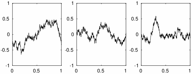
and (9) can be used directly in an implementation. We illustrate this in Figures 1 and 2 where three realizations of $X_{T}(\omega)$, $\omega\in\Omega$, are calculated approximatively with the numerical approximation method (4) in the case where $T=1$, $n=10000$, $h_{n}=1/\sqrt{n}$, $\varrho=\nicefrac{{5}}{{64}}$, $\chi=\nicefrac{{1}}{{128}}$, and $\xi=0$. The Matlab code used to generate Figure 1 can be found in Figure 2 below. The approximation scheme (4) is thus an easily implementable strongly convergent approximation method for the SPDE (3). In particular, to the best of our knowledge, the scheme (4) is the first approximation method in the scientific literature that has been shown to converge strongly to the solution of the stochastic K-S equation (3).

The remainder of this article is organized as follows. In Section 2 the required a priori moment bounds for the nonlinearity-truncated approximation schemes are established and in Section 3 the error analysis is performed in the pathwise sense under the hypothesis of suitable a priori bounds for the approximation processes. Section 4 combines the results of Section 2 and Section 3 and thereby establishes strong convergence in Theorem 4.6, which is the main result of this article. The analysis in Sections 2–4 is carried out for abstract stochastic evolution equations on separable Banach and Hilbert spaces, respectively. Section 5 then verifies that the assumptions of Theorem 4.6 in Section 4 are satisfied in the case of concrete stochastic partial differential equations of the type (3) and, in particular, establishes Corollary 5.10.

In this section we accomplish in Proposition 2.5 and Corollary 2.6 below appropriate a priori bounds for our approximation scheme. Before we establish Proposition 2.5 and Corollary 2.6 below, we present in Lemma 2.1, Lemma 2.2, Lemma 2.3, and Lemma 2.4 a few elementary auxiliary results for Proposition 2.5 and Corollary 2.6.

References

- [1] Becker, S., and Jentzen, A. Strong convergence rates for nonlinearity-truncated Euler-type approximations of stochastic Ginzburg-Landau equations. arXiv:1601.05756 (2016), 58 pages.
- [2] Blömker, D., and Jentzen, A. Galerkin approximations for the stochastic Burgers equation. SIAM J. Numer. Anal. 51, 1 (2013), 694–715.
- [3] Bogachev, V. I. Measure Theory. Vol. I, II. Springer-Verlag, Berlin, 2007.
- [4] Brzeźniak, Z., Carelli, E., and Prohl, A. Finite-element-based discretizations of the incompressible Navier-Stokes equations with multiplicative random forcing. IMA J. Numer. Anal. 33, 3 (2013), 771–824.
- [5] Cox, S., Hutzenthaler, M., and Jentzen, A. Local Lipschitz continuity in the initial value and strong completeness for nonlinear stochastic differential equations. arXiv:1309.5595 (2013), 88 pages.
- [6] Cox, S., Hutzenthaler, M., Jentzen, A., van Neerven, J., and Welti, T. Convergence in Hölder norms with applications to Monte Carlo methods in infinite dimensions. arXiv:1605.00856 (2016), 38 pages.
- [7] Da Prato, G., and Zabczyk, J. Stochastic equations in infinite dimensions, vol. 44 of Encyclopedia of Mathematics and its Applications. Cambridge University Press, Cambridge, 1992.
- [8] Duan, J., and Ervin, V. J. On the stochastic Kuramoto-Sivashinsky equation. Nonlinear Anal. 44, 2, Ser. A: Theory Methods (2001), 205–216.
- [9] Graham, C., and Talay, D. Stochastic simulation and Monte Carlo methods, vol. 68 of Stochastic Modelling and Applied Probability. Springer, Heidelberg, 2013. Mathematical foundations of stochastic simulation.
- [10] Gyöngy, I., and Millet, A. On discretization schemes for stochastic evolution equations. Potential Anal. 23, 2 (2005), 99–134.
- [11] Gyöngy, I., Sabanis, S., and Šiška, D. Convergence of tamed Euler schemes for a class of stochastic evolution equations. Stoch. Partial Differ. Equ. Anal. Comput. (2015), 1–21.
- [12] Henry, D. Geometric theory of semilinear parabolic equations, vol. 840 of Lecture Notes in Mathematics. Springer-Verlag, Berlin, 1981.
- [13] Hu, Y. Semi-implicit Euler-Maruyama scheme for stiff stochastic equations. In Stochastic analysis and related topics, V (Silivri, 1994), vol. 38 of Progr. Probab. Birkhäuser Boston, Boston, MA, 1996, pp. 183–202.
- [14] Hutzenthaler, M., and Jentzen, A. Convergence of the stochastic Euler scheme for locally Lipschitz coefficients. Found. Comput. Math. 11, 6 (2011), 657–706.
- [15] Hutzenthaler, M., and Jentzen, A. Numerical approximations of stochastic differential equations with non-globally Lipschitz continuous coefficients. Mem. Amer. Math. Soc. 4 (2015), 1–112.
- [16] Hutzenthaler, M., Jentzen, A., and Kloeden, P. E. Strong and weak divergence in finite time of Euler’s method for stochastic differential equations with non-globally Lipschitz continuous coefficients. Proc. R. Soc. Lond. Ser. A Math. Phys. Eng. Sci. 467 (2011), 1563–1576.
- [17] Hutzenthaler, M., Jentzen, A., and Kloeden, P. E. Strong convergence of an explicit numerical method for SDEs with non-globally Lipschitz continuous coefficients. Ann. Appl. Probab. 22, 4 (2012), 1611–1641.
- [18] Hutzenthaler, M., Jentzen, A., and Kloeden, P. E. Divergence of the multilevel Monte Carlo Euler method for nonlinear stochastic differential equations. Ann. Appl. Probab. 23, 5 (2013), 1913–1966.
- [19] Jentzen, A. Stochastic Partial Differential Equations: Analysis and Numerical Approximations. Lecture notes, ETH Zurich, summer semester 2015, available online at https://people.math.ethz.ch/~grsam/NASPDE_MATH_FS15/script/NASPDE_130.pdf, September 2015.
- [20] Jentzen, A., and Kloeden, P. E. The numerical approximation of stochastic partial differential equations. Milan J. Math. 77, 1 (2009), 205–244.
- [21] Jentzen, A., and Kloeden, P. E. Overcoming the order barrier in the numerical approximation of stochastic partial differential equations with additive space-time noise. Proc. R. Soc. Lond. Ser. A Math. Phys. Eng. Sci. 465, 2102 (2009), 649–667.
- [22] Jentzen, A., Kloeden, P. E., and Winkel, G. Efficient simulation of nonlinear parabolic SPDEs with additive noise. Ann. Appl. Probab. 21, 3 (2011), 908–950.
- [23] Jentzen, A., and Pušnik, P. Strong convergence rates for an explicit numerical approximation method for stochastic evolution equations with non-globally Lipschitz continuous nonlinearities. arXiv:1504.03523 (2015), 38 pages.
- [24] Kloeden, P. E., and Neuenkirch, A. The pathwise convergence of approximation schemes for stochastic differential equations. LMS J. Comput. Math. 10 (2007), 235–253.
- [25] Kovács, M., Larsson, S., and Lindgren, F. On the discretization in time of the stochastic Allen-Cahn equation. arXiv:1510.03684 (2015), 34 pages.
- [26] Kurniawan, R. Numerical approximations of stochastic partial differential equations with non-globally Lipschitz continuous nonlinearities. Master thesis, University of Zurich and ETH Zurich (2014), 74 pages.
- [27] Lord, G. J., and Tambue, A. Stochastic exponential integrators for the finite element discretization of SPDEs for multiplicative and additive noise. IMA J. Numer. Anal. 33, 2 (2013), 515–543.
- [28] Prévôt, C., and Röckner, M. A concise course on stochastic partial differential equations, vol. 1905 of Lecture Notes in Mathematics. Springer, Berlin, 2007.
- [29] Qi, R., and Wang, X. An accelerated exponential time integrator for semi-linear stochastic strongly damped wave equation with additive noise. arXiv:1602.06050 (2016), 20 pages.
- [30] Sabanis, S. A note on tamed Euler approximations. Electron. Commun. Probab. 18 (2013), no. 47, 1–10.
- [31] Sabanis, S. Euler approximations with varying coefficients: the case of superlinearly growing diffusion coefficients. arXiv:1308.1796 (2015), 24 pages.
- [32] Stroock, D. W. Probability Theory, second ed. Cambridge University Press, 2010. Cambridge Books Online.
- [33] Tretyakov, M. V., and Zhang, Z. A fundamental mean-square convergence theorem for SDEs with locally Lipschitz coefficients and its applications. SIAM J. Numer. Anal. 51, 6 (2013), 3135–3162.
- [34] Wang, X., and Gan, S. The tamed Milstein method for commutative stochastic differential equations with non-globally Lipschitz continuous coefficients. J. Difference Equ. Appl. 19, 3 (2013), 466–490.
- [35] Wang, X., and Qi, R. A note on an accelerated exponential Euler method for parabolic SPDEs with additive noise. Applied Mathematics Letters 46 (2015), 31–37.