Heterogeneous diffusion, viscosity and the Stokes Einstein relation in binary liquids
Abstract
We investigate the origin of the breakdown of the Stokes-Einstein relation (SER) between diffusivity and viscosity in undercooled melts. A binary Lennard-Jones system, as a model for a metallic melt, is studied by molecular dynamics. A weak breakdown at high temperatures can be understood from the collectivization of motion, seen in the isotope effect. The strong breakdown at lower temperatures is connected to an increase in dynamic heterogeneity. On relevant timescales some particles diffuse much faster than the average or than predicted by the SER. The van-Hove self correlation function allows to unambiguously identify slow particles. Their diffusivity is even less than predicted by the SER. The time-span of these particles being slow particles, before their first conversion to be a fast one, is larger than the decay time of the stress correlation. The contribution of the slow particles to the viscosity rises rapidly upon cooling. Not only the diffusion but also the viscosity shows a dynamically heterogeneous scenario. We can define a “slow” viscosity. The SER is recovered as relation between slow diffusivity and slow viscosity.
pacs
64.70.pe,66.10.-x,66.20.-dI Introduction
Diffusivity and shear viscosity largely characterize the dynamics of liquids. The shear viscosity is a macroscopic measure of the resistance of the fluid against shear deformation whereas the diffusion coefficient measures the long range atomic motion. Far above the liquidus temperature the atomic quantity and the macroscopic are connected by the Stokes-Einstein relation (SER):[1]
| (1) |
where is the temperature, an effective radius of the particle, is the Boltzmann constant and the constant varies between 4 and 6 depending on slip or stick boundary between particle and fluid. The SER is derived for the diffusion of uncorrelated macroscopic spheres in a liquid. Treating the motions of the solvent atoms as uncorrelated the SER is also applied to the diffusion of single atoms or molecules at high temperatures. Discrepancies of up to 20% can be absorbed in an effective hydrodynamic radius and a change of the boundary condition from stick to slip.[2] In the absence of values of either or the SER is often employed to estimate the missing quantity. It has been widely used in fields as distinct as transport in cells[3, 4] and magma flow [5, 6]. Molecular transport is treated by using an effective hydrodynamic radius in Eq. (1). The shape of small molecules can be included by replacing the Stokes formula for spheres by the one for ellipsoids.[7] Some effects of collective motion can be included by accounting for the wave vector dependence of the velocity field leading to a generalized SER.[2, 8]
The viscosity is not always known, or is difficult to compute and, therefore, the structural relaxation time is often used as an alternative to study the temperature dependence. This alternative equation is frequently referred to as Stokes-Einstein-Debye relation (SEDR), assuming
| (2) |
The proportionality holds approximately, but breaks down even for simple binary glasses as the temperature is lowered.[9]
It has been shown both in experiment [10, 11, 12, 13, 14, 15, 16, 17, 18] and simulation [19, 20, 21, 22, 23, 24, 25, 26, 27, 28, 29, 30, 31, 32, 9, 33, 34, 35] that upon cooling towards the glass transition the SER breaks down, the diffusivity remaining much larger than estimated via the SER or SEDR from the increase in viscosity or relaxation time. These experiments and simulations report mostly a breakdown in the SER about 30% above the glass transition temperature or in the region of the critical temperature of mode coupling theory[36]. Both measurements of metallic glasses [15, 18] and computer simulations [28, 30, 31, 33, 35] have however shown that there is already a weaker breakdown of the SER at much higher temperatures. This has been attributed to an increase of cooperativity.
To account for deviations from the SER, an empirical modification, fractional SER,has been proposed, where is replaced by with .[37] A number of theories predict fractional SER’s or SEDR’s. There is no consent on the value of the fractional exponent . It has been argued that such deviations from should be taken as a hint to look for effects beyond hydrodynamics which affect or exponentially.[38] One such effect could be the increased collectivity of motion. In that temperature range, barriers in configuration space start to dominate the dynamics. Hopping motion becomes visible and eventually dominates over flow. Consequently the diffusion coefficient rises above its SER-value. Concentrating on hopping motion between deep energy minima (meta-basins) Heuer and coworkers found for a fractional SEDR exponents as low as .[39] Considering fluctuations in the heights of barriers in the hopping dynamics of a colloidal system larger values of have been reported.[40] Similar values are obtained in a model where one treats fluctuations in the time between hops, persistence times, again similar exponents are gained. These values are in good agreement with experiments.[11, 16] In a simulation treating fluctuations of jamming of atomic mobility a similar exponent, , was found.[41] Another argument for a fractional SER exponent can be given using Adam-Gibbs theory arguing that the activation free energies of diffusion and viscosity are differently influenced by configurational entropy.[33]
A fractional SER can also be derived from the coupling model[42].
In an experiment on Zr64Ni36 upon cooling a transition from the SER dependence to has been observed. It was rationalized from Mode coupling theory[36] (MCT) that describes the transition from a flow motion dominated by binary collisions to one dominated by collective motion.[18] Surprisingly this transition sets in at a temperature far above the MCT critical temperature, even above the liquidus temperature. Including spatially heterogeneous relaxations in MCT again a fractional SER is found.[43]
The low temperature breakdown of the SER is mostly ascribed to the dynamic heterogeneity that abruptly grows at similar temperatures. To quantify the effect has proved rather elusive and often somewhat arbitrary definitions of fast and slow particles have been used. Particles are often divided into fluid or solid types. Solid type particles diffuse via hopping motion which is often regarded as nearest neighbor hopping. For a hard sphere model with density above the MCT critical density it was argued that the breakdown is due to particles that hop over distances that are integers of the particle spacing (solid like particles).[27] Alternatively the appearance of secondary peaks in the self correlation function is used.[34] These secondary peaks are mainly observed for small minority components. We will show that the SER breakdown also occurs for the majority component where no secondary peak is found and which dominates the viscosity. In agreement with the experimental results on diffusion in metallic melts[44] no typical length scale was found in simulations of CuZr.[45] Hopping motion can be identified but does not involve a definite length scale and in general cannot easily be identified from the atomic self correlation function. In a metallic melt, jump processes are typically not jumps between localized sites but jumps of strings of atoms.[44]
In composite liquids the breakdown of the SER occurs in general at different temperates for the different components.[29, 30] It has been argued that the breakdown of the SER is directly related to a dynamical decoupling of the components.[29] Such decoupling is in contradiction to the picture of collective string motion. Changes in dynamics, however, do affect the two components differently and quantities such as the ratio of the diffusion coefficients can be used as marker.[30, 35]
In the following we present a molecular dynamics study of a binary Lennard-Jones system for temperatures down to approximately the MCT critical temperature. After giving calculational details we evaluate the diffusion coefficients and the viscosity and find a breakdown of the SER. From the ratio of the component diffusion coefficients we find two transition temperatures, first weak break around and then a strong violation of the SER near . We then establish that diffusion in the relevant temperature interval is collective and that heterogeneity rapidly rises at the low temperatures. The van-Hove self correlation function is used to identify slow particles without using ad hoc cutoffs. The evolution of the slow particle contribution defines a slow diffusion coefficient and the lifetime of a particle staying slow. This time is larger than the average stress correlation time. Like the diffusion the viscosity is subject to a dynamically heterogeneous scenario. For a virtual fluid, formed by these slow particles only, the SER is recovered.
II Calculational details
The simulations were done for binary systems of 5488 atoms with a ratio of 4:1 between A- and B-atoms. The atoms interact via a binary Lennard-Jones potential described by
| (3) |
where the subscripts denote the two species A and B. The potential cutoff was set at . As the parameters, we took the values of Kob and Andersen [46]: , , , and . The parameters and ensure continuity of the potential and its first derivative at the cutoff. All masses are set to . As usual, in the following, we will give all results in the reduced units of energy , , and atomic mass. To compare with real metallic glasses one can equate one time unit () roughly to 1 ps. The time step is . At the higher temperatures the time step was reduced to and . The calculations were done with periodic boundary conditions at constant volume, where the volume at each temperature was fixed to give an average pressure, after aging, of . The heat bath is simulated by comparing the temperature averaged over 20 time steps with the nominal temperature. At each time step 1% of the temperature difference is adjusted by random additions to the particle velocities. Apart from the very first steps of the aging procedure the correction, after excursions of the temperature due to relaxations, does not exceed of the average velocity. This procedure assures that existing correlations between the motion of atoms are only minimally affected. The investigated temperatures ranged from to . The samples were aged at the high temperature then rapidly quenched to the next lower temperature and again aged. Apart from small residual effects at the lowest temperatures and no significant effect of not sufficient aging was observed. We used 8 independent samples. To improve the statistics for some calculations, e. g. the diffusional isotope effect and viscosity, these samples were split, after aging, into up to 250 sub-samples each. These were subsequently aged for a shorter time span.
III Calculation
III.1 Diffusion
We calculate the diffusion coefficients from the long time evolution of the mean square displacements using the standard expression
| (4) |
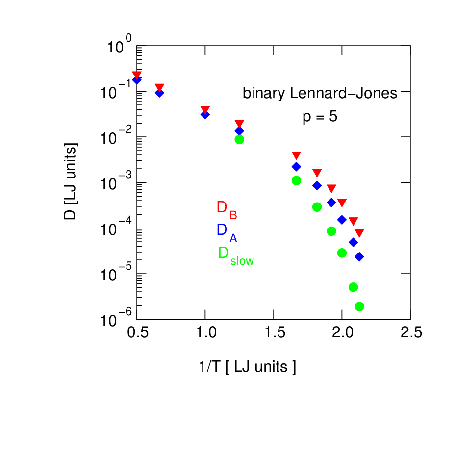
where indicates the average over all atoms of species and all samples. Fig. 1 shows for both A- and B-atoms the usual behavior. At high temperature the diffusivity follows with temperature an Arrhenius law. As predicted by MCT or a Vogel-Fulcher-Tamann (VFT) relation, at lower temperatures the diffusivities drop rapidly below their respective Arrhenius values. The onset temperature for this drop is for both components. The temperature range of the present investigation does not allow an unambiguous identification of low temperature VFT or MCT laws. The MCT critical temperature is . Additionally, we show in the figure values of the slow diffusion contribution (), which we will discuss further down. To get an estimate for the timescale of diffusional motion we define a diffusional time, as the time in which the average mean square displacement increases, according to Eq. (4), by . In the temperature interval from to this diffusional time of the A-atoms increases from by four orders of magnitude to about 7000. The values of are given in Fig. 14 further down.
It has been argued [30, 35] that in binary metallic melts the temperature dependence of the ratio of the diffusion coefficients of the two components is a sensitive probe of the change in dynamics which affects the two components differently. According to Fig. 2 the present system shows three temperature regimes. At high temperatures () the two diffusion coefficients evolve in parallel. In an intermediate regime () the ratio increases with . Finally, below the ratio increases rapidly. The high temperature regime as expected for simple liquid when diffusion is dominated by binary collisions and back-flow effects or chemical bonds are not too important. The ratio is given by the inverse ratio of the effective atomic radii. In this temperature regime the SER is expected to hold.
In the other two temperature regimes one expects first a weak deviation and then a catastrophic breakdown of the SER. This will be discussed further down.

III.2 Viscosity
We calculate the shear viscosity, , from the Green-Kubo relation as time integral over the stress auto-correlation function [47]:
| (5) |
with
| (6) |
where is the simulation volume and stands for the off-diagonal elements of the macroscopic stress tensor computed from the momenta and virials
| (7) |

Fig. 3 shows the time evolution of the Green-Kubo integral for temperatures from down to . AS an additional check of the reliability of our results we compared them for all temperatures to the values obtained for sets of different samples which were fully independent of the ones used in the present study. These control calculations were done using the LAMMPS program package.[48] The agreement was always within 5%. We are concentrating in this work on the strong violation of the SER at lower temperature where it is Larger by orders of magnitude.

The blue diamonds in Fig. 4 show the viscosity calculated from Eq. (5). As characteristic for metallic melts, two temperature regimes can be distinguished: a slow increase upon cooling at high temperatures and a much more rapid one at lower temperatures. The strength of the change of the asymptotic slopes shows that our system can be classified as fairly fragile. By extrapolation we find a crossover temperature of in good agreement with the onset temperature found for diffusion. The transition from high to low temperature viscosity spans the temperature interval . This corresponds roughly to the intermediate regime in , Fig. 2.
III.3 Stokes Einstein Relation
Combining the diffusion and viscosity data we can now calculate the SER, Eq. (1). In Fig. 5 we plot against inverse temperature. The SER holds as long as remains constant, independent of temperature. In agreement with the constant ratio the SER holds for temperatures down to about for both components. Below one clearly observes a rapid increase. The intermediate region is not seen unambiguously. For the larger A-atoms the relation holds approximately the temperature interval (open blue diamonds in the insert). This agrees with the experimental observation of Brillo et al. [18] and simulations for CuZr[30, 31]. For the smaller B-atoms this transition interval seems shifted to higher temperatures (not shown). It has been argued that the near constancy of is a signature of collective flow as described by MCT. However, a fractional SER, , (solid blue diamonds in the insert) holds in the shifted temperature interval . This value of is in good agreement to experiments on small organic molecules.[11, 16]. The present data are insufficient to clearly identify the proper relation in this higher temperature range ().

Also shown in the figures are values for slow atoms. This will be explained in the following section where we discuss the evolution of diffusion and viscosity with temperature in more detail.
IV Discussion
To gain more insight into the breakdown of the SER we take a closer look at both diffusion and viscosity. Main reasons for the breakdown, discussed in the literature, are increases of both collectivity and dynamic heterogeneity upon cooling. To quantify the collectivity of diffusion we use the isotope effect and for the dynamic heterogeneity the non-Gaussianity. Having established these we turn to the van-Hove self correlation function that allows separation of slow and fast diffusional motion. Separating the different contributions to the stress auto-correlations we find the contributions of slow and fast atoms to the viscosity. The different processes governing diffusion and viscosity are essentially on different time-scales. Comparing these is essential in understanding the SER in undercooled liquids.
IV.1 Isotope effect
At high temperatures and low densities, diffusion in liquids is dominated by binary collisions. The kinetic approximation for the mass dependence of the diffusion constant, , holds. When the temperature is lowered or the density is increased, effects of collective motion gain importance and the diffusional mass changes to an effective mass, . A frequently used measure of this collectivization is the isotope effect parameter [49]
| (8) |
where denotes the different components and and denote different isotopes. Using radio-tracer isotopes of Co values of or less have been measured in metallic glasses and supercooled metallic melts [50, 51]. These low values, compared to the typical value of for vacancy diffusion in crystals, is taken as strong evidence of a collective process. Due to experimental difficulties no systematic study of the temperature dependence is available. Using large mass differences, early molecular dynamics simulations for hard disks and LJ-systems found again small isotope effects [52, 53, 54, 55]. Using small mass differences, simulations of monotonic and binary LJ-systems at pressure gave a drop from at high temperatures to approaching the glass transition.[56, 57].
We repeated these calculations for the present system that has a shorter cutoff and is under high pressure, . We changed the the mass of small randomly chosen subsets of A- and B-atoms, each comprising 1.8% of the species, by . The average mass was thus kept constant. Due to the small concentrations clustering effects should not be important. For all 6 atom species (A and B, average mass, heavy and light) the diffusion coefficient was calculated and was evaluated. The mass change was . Additional test runs with and showed no significant difference. Starting point were the 8 samples which had been aged before the calculation of the diffusion coefficients, Fig. 1. To gain sufficient statistics for each of these 8 samples at least 1000 sets with changed mass were created and evaluated. A conservative estimate of the resulting uncertainty is about 10% and 20% for the A- and B-atoms,respectively.

Fig. 6 shows a behavior similar to the zero pressure system. The shorter cutoff reduces the collectivity slightly. In the previous calculations we have shown that the isotope effect of the majority component A is essentially given by the density alone. For the minority component B such a scaling with only the density is, however, not valid. There is both a temperature and density dependence. In general one cannot expect a pure density scaling for tracer atoms in a multi-component system.

The isotope effect can be used to estimate the number of atoms effectively participating in the elementary process of diffusion. We write the effective diffusional mass as
| (9) |
where stands for the effective number of atoms moving cooperatively and is the average atomic mass, in our case . Inserting the effective mass into Eq. (8) one finds . From Fig. 6 we deduct that there is already considerable collectivity at the onset temperature and it increases to more than below . Converting this into a correlation length by we get a correlation length which coincides with the length calculated from the four-point correlation. If one attributes the isotope effect to string- or chain-like motion by we get a chain length . Here we assumed an effective dimension of for the chain.[58]
The temperature dependence of does not show any pronounced feature in Fig. 6. The change in dynamics is however reflected in the inverse isotope effect , Fig. 7. The rapid increase in collectivity in the diffusion of the A-atoms at low temperatures is evident. Whether the change in dynamics around observed in Fig. 2 is also reflected in is beyond our accuracy. The same holds for the ratio in Fig. 6. The isotope effect does not give direct information on the nature of collectivity. Values of can still be imagined as originating from weakly correlated pushing in the dense liquid. However, that is not likely for values or . It is well established that in undercooled densely packed metallic liquids collective motion by chain- (string-)like structures becomes dominant.[59, 60, 61] Such mobile chains are the main contributor to the dynamic heterogeneity.
IV.2 Non-Gaussianity
In glasses and undercooled melts the mobility of the atoms varies in time, the so called dynamic heterogeneity. Two approaches are commonly used to describe this phenomenon. Placing the emphasis on the slow particles, four point correlations of displacement or overlap functions are studied and the dynamic heterogeneity is defined from the dynamic susceptibility [62, 63]. Alternatively one quantifies the deviations from Gaussian distributions of displacements, typical for homogeneous diffusion. We adopt the latter approach due to its direct connections to the van-Hove self correlation and to diffusion where the weight is on the fast particles.
We define a non-Gaussianity parameter [64]
| (10) |
For a purely homogeneous motion . For heterogeneous motion increases with time. Since undercooled melts are ergodic and in the long time limit homogeneous, for .

Fig. 8 shows the general behavior expected from numerous earlier simulations. At short times () there is a small increase to around 0.1 due to the inhomogeneity of the vibrational spectrum. This increase shows little temperature dependence. For longer times the non-Gaussianity first increases rapidly, as shown previously[65] , goes through a maximum and finally decays as . The dynamics of the smaller B-atoms is much faster than the one of the A-atoms and the heterogeneity is larger. However, for long times their values decay to the corresponding ones of the A-atoms which shows that the dynamics of the A- and B-particles is coupled. We define a non-Gaussianity time as the time when reaches its maximum value . For the majority A-particles, by scaling with and , the curves of for the different temperatures can be collapsed to a master curve. The scaling does not fully account for the detailed shape of the maxima. Considering the change in collectivity with temperature, discussed above, this is not too surprising. The scaling implies that the maximum value of for a given temperature increases with the time the maximum is reached. For the A-particles we show in Fig. 14 further down. For temperatures below , the times increase rapidly and reach at values of 430 and 150, for the A and B particles, respectively. These times are one order of magnitude less than the diffusion times . The dynamic heterogeneity reaches its maximum long before the particles have on average diffused over appreciable distances. We have previously shown [65], that the time dependencies of can be explained by collective chain- (string-)dynamics. This dynamics involves two times, one defining the mobility of the chains, the other the decay of the chains. The times result from an interplay of these two. One can imagine the heterogeneous dynamics as strings of particles moving in a slow environment. The fast strings will loose from time to time particles, most likely at the ends, to the slow environment. To compensate they will pick up new particles. Moving strings also trigger the formation of new strings or disintegrate. Both scenarios lead to a correlation between moving particles[44] and cause a transition from slow to fast particle and vice versa.
IV.3 Van-Hove self correlation function
The time dependent distribution of the displacements of single atoms can be expressed by the van-Hove self correlation function (vHSCF). In an isotropic system it can be averaged over the space angle to give
| (11) |
where is the position of atom at time . is a probability function whose space integral is time independent equal unity. It is usually plotted as . For the vHSCF is a -function at . With time the atoms are displaced and the vHSCF broadens. In a purely homogeneous system the vHSCF keeps its Gaussian shape, the non-Gaussianity , Eq. (10). Vibrations and ballistic motion lead to a small broadening which rapidly saturates in time, the deviation from a Gaussian shape is small, Fig. 8. For long times the system becomes homogeneous again and the vHSCF is determined by the diffusion coefficient
| (12) |
At intermediate times, when the non-Gaussianity parameter is large, one observes a strong deviation from the Gaussian shape. Such deviations are typical for many disordered systems.[66] This is the time region which is of main interest in the present investigation. As example Fig. 9 shows the the time evolution at of the vHSCF for both components.

It shows the evolution with time of long range tails of the vHSCF for both components. At the often observed secondary peak around becomes visible for the B-atoms. For the A-atoms there might be traces of a shoulder. In a simulation of CuZr it has been shown that the secondary peak is not due to a preferred jump length, but is due to increased residence times at previous nearest neighbor sites.[56]. The secondary peak forms at times comparable to the “diffusion time”, , but long after the non-Gaussianity has passed its maximum value at . For the long range tails become part of a strongly broadened Gaussian given by Eq. (12). We plot against . In such representation a Gaussian is seen as a straight line.


As example Fig. 10 shows a logarithmic plot for the A-atoms at and at different times. In this representation Gaussians are seen as straight line which level off with time. The actual values of the vHSCF for larger distances lie above this straight line, indicating an enhanced mobility of some atoms. The slower than Gaussian decay of the vHSCF at larger distances reflects the tails in Fig. 9. With increasing time this enhancement vanishes as can be seen for at the two later times. The calculated vHSCF nearly coincides with its Gaussian asymptote, in agreement with the vanishing non-Gaussianity (Fig. 8). However even when there is a strong curvature in the calculated values, the central part still shows a Gaussian shape which persists at the lower temperature to long times (). The generally accepted picture of the dynamic heterogeneity is that at any time there are slow and fast atoms which exchange their roles with time and thus preserve homogeneity in the long time limit. At short times, the central, Gaussian part of the vHSCF is comprised mainly of those atoms which have no fast history.
We fit this central part of the vHSCF by a Gaussian. The fit is done for to . The width of the central Gaussian is given by the sum of vibration or ballistic motion, cage motion and slow-diffusion. The first two contributions become constant after some initial time whereas the diffusional part increases as . We write
| (13) |
Here gives the fraction of atoms contained in the central peak. These are essentially the atoms which have not jumped (have not been fast atoms). Such fits were done for temperatures ranging from 0.47 to 2.0. The slow atom Gaussians are given as green straight lines in Fig. 10. The width B(t) can be written as
| (14) |
Here the constant accounts for vibrational, ballistic and cage motion which are supposed to be fast on the diffusional time scales. The above decomposition can only be done when there is a sufficient time interval during which the slow motion of atoms persists before these atoms convert into “fast” ones. In our case we can evaluate Eq. 14 for temperatures below . Eq. 14 can only be used as long as the majority of atoms is still . From Fig. 10 and the equivalent Figs. for the other temperatures we estimate an accuracy of about 5% for the asymptotic . If one does the fit formally to long times will transform with time into the long time diffusion coefficient .

This time evolution of the Gaussian width of the vHSCF, as calculated from its central part, is exemplified in Fig. 11. It shows for both components the changeover from “slow diffusion” to normal diffusion. Neglecting dynamic heterogeneity and doing Gaussian fits for the vHSCF on some not too long timescale can give apparent diffusion coefficients varying between the slow value and the long time diffusion coefficient. Thus values of the diffusivity, which are derived by a Gaussian approximation, depend on measuring time, fit range and weighting factors.
At short times the width for A and B particles coincide within our accuracy. This indicates a strong cooperativity in this temperature range, in agreement with the above results of non-Gaussianity and isotope effect.
The slow diffusion coefficients derived from Eq. (14) are shown in Fig.1 by green circles. The drop of from the Arrhenius values is much more pronounced than the one of the average long time coefficients. At i is one order of magnitude smaller than . The product strongly drops below the constant value predicted by the SER, shown by green circles in Fig. 5. We cannot verify the claim, sometimes made, that the SER holds for the slow particles. To restore the validity of the SER one could introduce an appropriate definition of “slow” by either prescribing a timescale for the fit of the vHSCF or by using appropriate cutoff radii. We take a different approach and consider the heterogeneity of as well as of .
As mentioned before an essential parameter characterizing the heterogeneous dynamics is the conversion rate from slow to fast. The decay of the amplitude of the central Gaussian can be used to extract this rate. For short times the decay is given by
| (15) |
A value indicates that all atoms are in the central Gaussian. Fast cage hopping and heterogeneity of vibration and ballistic motion reduce the factor. As the central Gaussian merges with time into the long time diffusional Gaussian so does after the initial decay increase again to one. The amplitude initially decays exponentially indicating the rate of the transformation of slow particles into fast ones. Assuming that this is correlated to jumps, chains of atoms losing atoms and picking up others, this gives an estimate of the jump rate. An example of the time dependence of the central Gaussian is shown in Fig. 12. The conversion time increases in the temperature interval by two orders of magnitude, see Fig. 14. It is much larger than the non-Gaussianity time but smaller than the diffusion time. Fig. 11 shows that the central Gaussian showing the slow diffusion is clearly visible for time up to and even above .

IV.4 Viscosity time and partial viscosities
The Green-Kubo expression for the viscosity offers two advantages. First, one can study the time evolution of the Green-Kubo integral Eq. (5)
| (16) |
and thus define a time during which the stresses are sufficiently correlated to contribute to . To quantify the time-span during which the major part of is accumulated we define a viscosity time as
| (17) |
Secondly the sums in Eq. (5) can be split to show the contributions of different groups of atoms to .

The time evolution of is shown for two examples in Fig. 13 (solid black line). From these time evolutions we gain shown as red up-triangles in Fig. 14. It shows that the stress correlation decays faster, the viscosity evolves faster, than the conversion of a slow particle to a fast one, , whence the stress evolution is heterogeneous. Slow environments remain slow over relevant times. It is therefore useful to study the different contributions to separately. We introduce partial stress tensors for groups of atoms
| (18) |
and
| (19) |
where the index denotes all particles (total), all A or B particles (A or B), all slow A-particles or all fast A-particles. By definition . We count those A-atoms as slow which have been displaced least during the time . As we can determine only for temperatures , we only analyze the slow and fast contributions in that temperature range.
As example Fig 13 shows the normalized and some of the constituting terms for two temperatures. Not surprisingly we find that the viscosity of our system is dominated at all temperatures by the 80% A-particles. The contribution of the B-particles (B-total) is halved from about 12% at to at . We will, therefore, concentrate on the A-particles. Comparing the A-total and A-A terms one sees that the A-B contribution is nearly negligible. Since we have a ratio of 1.7 between the numbers of fast and slow A-atoms one expects in a homogeneous system a similar ratio for the fast-total and slow-total contributions to . This holds approximately at . But at the lower temperature the two contributions become comparable. Furthermore the slow-slow contribution becomes equal to the slow-total one, i.e. the slow A-atoms act as a subsystem. We use this to introduce a virtual slow system where all A-atoms are slow and contribute, as the slow atoms contribute in the real system. We substitute A-A slow-slow . The resulting viscosity of the virtual slow system is shown in Fig. 4 by green circles. It obeys approximately the SER. In this virtual system the stress correlations decays more slowly than in the real system, the virtual becomes similar to .
IV.5 Timescales
In Fig. 14 we summarize the different timescales encountered in this investigation and compare them with the -relaxation time . All timescales show the characteristic upturn at temperatures below . The time , which measures essentially the lifetime of the stress correlation entering the Green-Kubo relation for the viscosity, broadly coincides with . The maximum of the non-Gaussianity is reached on similar time scales. For the highest temperatures saturates when it is no longer dominated by diffusion and the non-Gaussianity is given by vibrational (ballistic) heterogeneity. At the low temperature side drops below as has been noted earlier [67]. With decreasing temperature the slow-diffusion time, , markedly diverges from the average diffusion time, , and from . The most interesting result is that the timescale for conversion from slow to fast A-particles, is larger than and the average . Dividing the atoms into slow and fast is therefore sensible on the timescales relevant for the buildup of the viscosity. There are of course some stress correlations over longer times, but these contribute only little to the viscosity. We want to stress that is not the same as the time a particle is a fast diffuser , as studied before[22]. The two times are related by an equilibrium condition for the concentration of slow and fast particles, . In the virtual system that consists only of slow A-particles is increased to approximately of the real system.

IV.6 Error-analysis
The accuracy of our results are affected by both limitations of the computations and by system immanent problems. The statistical errors can be estimated from the scatter of the data points in time as well as temperature. Due to the long aging times the samples at the different temperatures can be taken as fairly independent. We estimate the statistical error of the viscosity as less than 5% and for the partial viscosities as less than 10%. The diffusivities are calculated more accurately from the mean square displacements. At the lowest temperatures aging effects become noticeable.
It has been shown that at low temperatures there is a split between the aging rates of diffusivity and heterogeneity on one side and energy and pressure or volume on the other, with the second being the slower ones.[68] Viscosity presumably belongs to the slower aging group. Insufficient aging then might result in good values for the diffusivity but too low ones for the viscosity and as effect too low values of the SER. For our data this might have occurred for . Therefore we did not use this temperature in the final analysis but restricted to temperatures up from .
Both the calculated diffusion coefficients and the viscosities are affected by finite size effects which increase with lowering the temperature. These size effects are more pronounced for the diffusivities [69]. Simulation with different system sizes have shown that for our systems with 5488 particles the effect on the calculated SER is only marginal.
More important are the system immanent uncertainties of our calculation. We have introduced some times which define timescales but do not affect the actual calculations (, , , ). Inaccuracies in these numbers do not affect the general results. The conversation time from slow to fast () is more critical. It is determined from the values of the low asymptotes in Fig. 10. At the higher temperature () the time span between ballistic or vibrational motion and significant long range diffusion is too short for an accurate evaluation and we have omitted these values. According to Eq. (12) an error in the propagates with a factor 1.5 to . Apart from the lowest value we don’t expect the error to exceed a few percent.
The most critical step is the identification of the slow particles. During the relevant time for the viscosity a large number of particles are for some time “fast”. These particles also contribute to , Fig. 12, but should not be counted as “slow”. We have taken this into account by picking out these atoms which have moved least, including reversed jumps. Varying, in reasonable limits, and its fraction used to determine the SER for the slow system is changed by around 20%.
V Conclusion
Using molecular dynamics simulation of a binary Lennard-Jones melt we have investigated diffusion, viscosity and the Stokes-Einstein relation (SER), between them, as function of temperature. Three temperature regimes can be distinguished. At high temperatures the diffusion obeys an Arrhenius law, the viscosity is low and the SER holds (). Upon cooling the dynamics becomes increasingly collective but not yet strongly heterogeneous. In this intermediate temperature the SER is weakly violated. The relation between viscosity and diffusivity is often described by a fractional SER, .[37] For temperatures down to our results can be fitted with , in good agreement with experiments on organic liquids[11, 16]. As discussed in the introduction, fractional SER have been derived for numerous models accounting for hopping and fluctuations. As alternative a transition from the SER to a relation , emphasizing the growing collectivity, has been claimed.[18, 30, 31] The present data do not suffice to decide between the two description. The emphasis of this work is on the lower temperature region where the SER violation is much stronger and cannot be described by a fractional SER with a positive exponent .
At low temperatures approaching the glass transition the viscosity increases rapidly and the diffusion drops below the Arrhenius values, the SER is strongly violated, rapidly increases with . At the SER is violated by a factor of 2.5. The system shows both large dynamic heterogeneities and a strong collectivity of motion. We show that the strong violation of the SER results from the heterogeneity. With decreasing temperature viscosity becomes dominated by slow particles while diffusion is by fast particles. We share this picture with the majority of workers in the field. The definition of fast and slow often is limited to hopping motion. Other than in hard sphere systems, in metallic melts there is a smooth distribution of hopping distances and, therefore there is no clear identification of particles which have hopped.[45] As remedy sometimes a cutoff length in the van-Hove self-correlation (vHSCF) is used to separate slow and fast particles. The results for the SER depend crucially on this cutoff.
In the present work we show that slow and fast particles can be separated using the vHSCF. No distinction between hopping and flow motion is needed. At not too large times the vHSCF exhibits a Gaussian center. This is due to slow particles whereas fast ones are mainly seen in the non-Gaussian tails. The broadening of the central Gaussian with time measures a slow diffusivity. From the amplitude of the Gaussian we gain the lifetime of a particle as slow, before it undergoes a fast motion which takes it out of central Gaussian. This conversion time is longer than timespan during which the integral over the stress correlation contributes strongly in the Green Kubo formula to the viscosity. On the relevant time scales we observe a slow subsystem that with decreasing temperature more and more dominates the viscosity. It acts as a quasi static heterogeneity. Calculating an SER from the diffusivity of the slow particles and the viscosity leads to a dramatic underestimation of the SER values. Making a Gaussian approximation of the vHSCF over some distance would increase the SER ratio again. The SER can be regained without any implicit parameter when one considers the heterogeneity of both he stress correlation as of the diffusivity. In a virtual melt formed from the slow subsystem the SER is obeyed.
VI Acknowledgments
We are grateful to T. Voigtmann for many stimulating discussions throughout this work. HRS acknowledges the hospitality of the Institut für Materialphysik im Weltall at DLR, Cologne. The authors gratefully acknowledge the computing time granted on the supercomputer JUROPA at Jülich Supercomputing Center (JSC). The work was partially supported by the German Academic Exchange Servive (DAAD) through the DLR-DAAD programme under grant No. 131.
References
- [1] A. Einstein, Ann. Phys. 17, 549 (1905).
- [2] U. Balucani and M. Zoppi, Dynamics of the Liquid State (Clarendon Press, Oxford, 1994).
- [3] G. Clough, J. Physiol. 328, 389 (1982).
- [4] M.R. McCarthy, K.D. Vandegriff, and R. M. Winslow, Biophys. Chem. 94, 103 (2001).
- [5] J. P. Poirier, Geophys. J. 92, 99 (1988).
- [6] B. T. Poe, P. F. McMillan, D. C. Rubie, S. Chakraborty, J. Yarger, and J. Diefenbacher, Science 276, 1245 (1997).
- [7] F. Perrin, J. Phys. Radium 5, 497 (1934).
- [8] T. Gaskell, U. Balucani,and R. Vallauri, Phys. Chem. Liq. 19, 193 (1989).
- [9] Z. Shi, P. G. Debenedetti, and F. Stillinger, J. Chem. Phys. 138, 12A526 (2013).
- [10] E. Rössler, Phys. Rev. Lett. 65, 1595 (1990).
- [11] F. Fujara, B. Geil, H. Sillescu, and G. Fleischer, Z. Phys. B 88, 195 (1992).
- [12] M. T. Cicerone, F. R. Blackburn, and M. D. Ediger, J. Chem. Phys. 102, 471 (1995).
- [13] G. Heuberger and H. Sillescu, J. Phys. Chem. 100, 15255 (1996).
- [14] A. Voronel, E. Veliyulin, V. Sh. Machavariani, A. Kisliuk, and D. Quitmann, Phys. Rev. Lett. 80, 2630 (1998).
- [15] A. Meyer, W. Petry, M. Koza, and M.-P. Macht, Appl. Phys. Lett. 83, 3894 (2003).
- [16] S. F. Swallen, P. A. Bonvallet, R. J. McMahon, and M. D. Ediger, Phys. Rev. Lett. 90, 015901 (2003).
- [17] A. Bartsch, K. Rätzke, A. Meyer, and F. Faupel, Phys.Rev. Lett. 104, 195901 (2010).
- [18] J. Brillo, A. I. Pommrich, and A. Meyer, Phys. Rev. Lett. 107, 165902 (2011).
- [19] D. Thirumalai and R. D. Mountain, Phys. Rev. E 47, 479 (1993).
- [20] M. Nicodemi and A. Coniglio, Phys. Rev. E 57, R39 (1999).
- [21] L. Angelani, G. Parisi, G. Ruocco, and G. Viliani, Phys. Rev. Lett. 81, 4648 (1998).
- [22] R. Yamamotu and A. Onuki, Phys. Rev. E 58, 3515 (1999).
- [23] P. Allegrini, J. F. Douglas, and S. C. Glotzer, Phys. Rev. E 60, 5714(1999).
- [24] C. DeMichele and D. Leporini, Phys. Rev. E 63, 036701 (2001).
- [25] A. Mukherjee, S. Bhattacharyya, and B. Bagchi, J. Phys. Chem. 116, 4577 (2002).
- [26] P. Bordat, F. Affouard, M. Descamps, and F. Müller-Plathe, J. Phys.:Condens Matter 15, 5397 (2003).
- [27] S. K. Kumar, G. Szamel and J. F. Douglas, J. Chem. Phys. 124, 214501 (2006).
- [28] S. K. Das, J. Horbach, and T. Voigtmann, Phys. Rev. B 78, 064208 (2008).
- [29] F. Affouard, M. Descamps, L.-C. Valdes, J. Habasaki, P. Bordat, and K. L. Ngai, J. Chem. Phys. 131 104510 (2009).
- [30] X. J. Han and H. R. Schober, Phys. Rev. B 83, 224201 (2011).
- [31] X. J. Han and H. R. Schober, J. Chem. Phys. 144, 124505 (2016).
- [32] Y. Lü, H. Cheng, and M. Chen, J. Chem. Phys. 136, 214505 (2012). 138, 12A548 (2013).
- [33] S. Sengupta, S. Karmakar, C. Dasgupta, and S. Sastry, J. Chem. Phys.
- [34] S. Sengupta and S. Karmakar, J. Chem. Phys. 140, 224505 (2014).
- [35] A. Jaiswal, T. Egami, and Y. Zhang, Phys. Rev. B 91, 134204 (2015).
- [36] W. Goetze and L. Sjogren, Rep. Prog. Phys. 55, 241 (1992).
- [37] G. L. Pollack and J. J. Enyeart, Phys. Rev. A 31, 980 (1985).
- [38] R. Zwanzig and K. Harrison, J. Phys. Chem 83, 5861 (1985).
- [39] A. Heuer, J. Phys.: Condens. Matter 20, 373101 (2008).
- [40] K. S. Schweitzer and E. Saltzman, J. Phys. Chem. B 108, 19729 (2004).
- [41] Y. J. Jung, J. P. Garrahan, and D. Chandler, Phys. Rev. E 69, 061205 (2004).
- [42] K. L. Ngai Phil. Mag. B 79, 1783 (1999).
- [43] T. Rizzo and T. Voigtmann, EPL 111, 56008 (2015).
- [44] F. Faupel, W. Frank, M.-P. Macht, H. Mehrer, V. Naundorf, K. Rätzke, H. R. Schober, S. K. Sharma, and H. Teichler, Rev. Mod. Phys. 75,237 (2003).
- [45] M. Kluge and H. R. Schober, Phys. Rev. B 70, 224209 (2004).
- [46] W. Kob and H. C. Andersen, Phys. Rev. E 51, 4626 (1995). (Butterworts, London, 1984).
- [47] M. P. Allen and D. J. Tildesley, Computer Simulation of Liquids, (Clarendon Press, Oxford 1987).
- [48] http://lammps.sandia.gov.
- [49] A. H. Schoen, Phys. Rev. Lett. 1, 138 (1958).
- [50] F. Faupel, P. W. Hüppe, and K. Rätzke, Phys. Rev. Lett. 65, 1219 (1990).
- [51] H. Ehmler, A. Heesemann, K. Rätzke, F. Faupel, and U. Geyer, Phys. Rev. Lett. 80, 4919 (1998).
- [52] P. T. Herman and B. J. Alder, J. Chem. Phys. 56, 987 (1972).
- [53] I. Ebbsjö, P. Schofield, K. Sköld, and I. Waller, J. Phys. C 7, 3891 (1974).
- [54] R. J. Bearman and D. L. Jolly, Mol. Phys. 44, 665 (1981).
- [55] M. J. Nuevo, J. J. Morales, D. M. Heyes, Phys. Rev. E 51, 2026 (1995).
- [56] M. Kluge and H. R. Schober, Phys. Rev. E 62, 597 (2000).
- [57] H. R. Schober, Solid state Commun. 119, 73 (2001).
- [58] C. Oligschleger and H. R. Laird, Phys. Rev. B 59, 811 (1999).
- [59] H. R. Schober, C. Oligschleger, and B. B. Laird, J. Non-Cryst. Solids 156, 965 (1993).
- [60] H. R. Schober, C. Gaukel, and C. Oligschleger, Prog. Theor. Phys. Suppl. 126, 67 (1997).
- [61] C. Donati, J. F. Douglas, W. Kob, S. J. Plimplton, P. H. Poole, and S. C. Glotzer, Phys. Rev. Lett. 80, 2338 (1998).
- [62] C. Donati, S. C. Glotzer, and P. H. Poole, Phys. Rev. Lett. 82, 5064 (1999).
- [63] E. Flenner, M. Zhang, and G. Szamel, Phys. Rev. E 83, 051501 (2011).
- [64] A. Rahmann, Phys. Rev. 136, A405 (1964).
- [65] D. Caprion, J. Matsui, and H. R. Schober, Phys. Rev. Lett. 85, 4239 (2000).
- [66] P. Chaudhuri, L. Berthier, and W. Kob, Phys. Rev. Lett 99, 060604 (2007).
- [67] E. J. Saltzman and K. S. Schweitzer, Phys. Rev. E 74, 061501 (2006).
- [68] H. R. Schober, Phys. Rev. B 85, 024204 (2012).
- [69] I-C. Yeh and G. Hummer, J. Phys. Chem. B 108, 15873 (2004).