R-FUSE: Robust Fast Fusion of Multi-Band Images Based on Solving a Sylvester EquationThanks: Part of this work has been supported by the ERA-NET MED MapInvPlnt Project no. ANR-15-NMED-0002-02, by the Hypanema ANR Project no. ANR-12-BS03-003 and by ANR-11-LABX-0040-CIMI within the program ANR-11-IDEX-0002-02 within the thematic trimester on image processing. Thanks:  Qi Wei and Simon Godsill are with Department of Engineering, University of Cambridge, CB2 1PZ, Cambridge, UK (e-mail: {qi.wei, sjg}@eng.cam.ac.uk).Thanks:  Nicolas Dobigeon and Jean-Yves Tourneret are with University of Toulouse, IRIT/INP-ENSEEIHT, 2 rue Camichel, BP 7122, 31071 Toulouse cedex 7, France (e-mail: {nicolas.dobigeon, jean-yves.tourneret}@enseeiht.fr).Thanks:  José Bioucas-Dias is with Instituto de Telecomunicações and Instituto Superior Técnico, Universidade de Lisboa, Portugal (e-mail: {bioucas}@lx.it.pt).

The multi-band image fusion problem, i.e., fusing hyperspectral (HS) and multispectral (MS)/panchromatic (PAN) images has recently been receiving particular attention in remote sensing [2]. High spectral resolution multi-band imaging generally suffers from the limited spatial resolution of the data acquisition devices, mainly due to an unavoidable tradeoff between spatial and spectral sensitivities [3]. For example, HS images benefit from excellent spectroscopic properties with hundreds of bands but are limited by their relatively low spatial resolution compared to MS and PAN images (that are acquired in much fewer bands). As a consequence, reconstructing a high-spatial and high-spectral multi-band image from two degraded and complementary observed images is a challenging but crucial issue that has been addressed in various scenarios [4, 5, 6, 7]. In particular, fusing a high-spatial low-spectral resolution image and a low-spatial high-spectral image is an archetypal instance of multi-band image reconstruction, such as pansharpening (MS+PAN) [8] or hyperspectral pansharpening (HS+PAN) [2]. Generally, the linear degradations applied to the observed images with respect to (w.r.t.) the target high-spatial and high-spectral image reduce to spatial and spectral transformations. Thus, the multi-band image fusion problem can be interpreted as restoring a three dimensional data-cube from two degraded data-cubes. A detailed formulation of this problem is presented in the next section.

This work directly follows the formulation of [1] and uses the well-admitted linear degradation model

where

• •

  ${\mathbf{X}}\in\mathbb{R}^{m_{\lambda}\times n}$ is the full resolution target image,

• •

  ${{\mathbf{Y}}}_{\mathrm{L}}\in\mathbb{R}^{n_{\lambda}\times n}$ and ${{\mathbf{Y}}}_{\mathrm{R}}\in\mathbb{R}^{m_{\lambda}\times m}$ are the observed spectrally degraded and spatially degraded images,

• •

  ${{\mathbf{L}}}\in\mathbb{R}^{n_{\lambda}\times m_{\lambda}}$ is the spectral response of the sensor,

• •

  ${\mathbf{B}}\in\mathbb{R}^{n\times n}$ is a cyclic convolution operator on the bands,

• •

  ${\mathbf{S}}\in\mathbb{R}^{n\times m}$ is a $d=d_{r}\times d_{c}$ uniform downsampling operator, which has $m=n/d$ ones on the block diagonal and zeros elsewhere, such that ${{\mathbf{S}}}^{H}{\mathbf{S}}=\textbf{I}_{m}$,

• •

  ${\mathbf{N}}_{\mathrm{L}}\in\mathbb{R}^{n_{\lambda}\times n}$ and ${\mathbf{N}}_{\mathrm{R}}\in\mathbb{R}^{m_{\lambda}\times m}$ are additive noise terms that are assumed to be distributed according to the following matrix normal distributions [9]

  $$\begin{array}[]{ll}{\mathbf{N}}_{\mathrm{L}}\sim\mathcal{MN}_{m_{\lambda},m}(\boldsymbol{0}_{m_{\lambda},m},\boldsymbol{\Lambda}_{\mathrm{L}},\textbf{I}_{m})\\ {\mathbf{N}}_{\mathrm{R}}\sim\mathcal{MN}_{n_{\lambda},n}(\boldsymbol{0}_{n_{\lambda},n},\boldsymbol{\Lambda}_{\mathrm{R}},\textbf{I}_{n}).\end{array}$$

Computing the ML or the Bayesian estimators (associated with any prior) is a challenging task, mainly due to the large size of ${\mathbf{X}}$ and to the presence of the downsampling operator ${\mathbf{S}}$, which prevents any direct use of the Fourier transform (FT) to diagonalize the the joint spatial degradation operator $\bf{BS}$. To overcome this difficulty, several computational strategies have been designed to approximate the estimators. Based on a Gaussian prior, a Markov chain Monte Carlo (MCMC) algorithm was implemented in [10] to generate a collection of samples asymptotically distributed according to the posterior distribution of ${\mathbf{X}}$. The Bayesian estimators of ${\mathbf{X}}$ can then be approximated using these samples. Despite this formal appeal, MCMC-based methods have the major drawback of being computationally expensive, which prevents their effective use when processing images of large size. Relying on exactly the same prior model, the strategy developed in [11] exploits an alternating direction method of multipliers (ADMM) embedded in a block coordinate descent method (BCD) to compute the maximum a posterior (MAP) estimator of ${\mathbf{X}}$. This optimization strategy allows the numerical complexity to be greatly decreased when compared to its MCMC counterpart. Based on a prior built from a sparse representation, the fusion problem was solved in [12, 13] with the split augmented Lagrangian shrinkage algorithm (SALSA) [14], which is an instance of ADMM. In [1], contrary to the algorithms described above, a much more efficient method was proposed to solve explicitly an underlying Sylvester equation (SE) derived from (1), leading to an algorithm referred to as Fast fUsion based on Sylvester Equation (FUSE). This algorithm can be implemented per se to compute the ML estimator in a computationally efficient manner. The proposed FUSE algorithm has also the great advantage of being easily generalizable within a Bayesian framework when considering various priors. The MAP estimators associated with a Gaussian prior similar to [10, 11] can be directly computed thanks to the proposed strategy. When handling more complex priors such as [12, 13], the FUSE solution can be conveniently embedded within a conventional ADMM or a BCD algorithm. Although the FUSE algorithm has significantly accelerated the fusion of multi-band images, it requires the non-trivial assumption that the blurring matrix ${\mathbf{B}}$ is invertible, which is not always guaranteed in practice.

In this work, we propose a more robust version of FUSE algorithm, which is termed as R-FUSE. In this R-FUSE, the FT of the target image, instead of its blurring version as in [1], is computed explicitly by exploiting the Woodbury formula. A direct consequence of this modification is getting rid of the invertibility assumption for the blurring matrix ${\mathbf{B}}$. A side product of this modification is that the permutations conducted in the frequency domain (characterized by the matrix ${\mathbf{P}}$ in [1]) are no longer required in the R-FUSE algorithm.

Minimizing (2) w.r.t. ${\mathbf{U}}$ is equivalent to force the derivative of $L({\mathbf{U}})$ to be zero, i.e.,$\nabla L({\mathbf{U}})=0$, leading to the following matrix equation

As mentioned in Section I-B, the difficulty for solving (3) results from the high dimensionality of ${\mathbf{U}}$ and the presence of the downsampling matrix ${\mathbf{S}}$. The work in [1] showed that Eq. (3) can be solved analytically with two assumptions

• •

  The blurring matrix ${\mathbf{B}}$ is a block circulant matrix with circulant blocks.

• •

  The decimation matrix ${\mathbf{S}}$ corresponds to downsampling the original image and its conjugate transpose ${\mathbf{S}}^{H}$ interpolates the decimated image with zeros.

As a consequence, the matrix ${\mathbf{B}}$ can be decomposed as ${\mathbf{B}}={\mathbf{F}}{\mathbf{D}}{\mathbf{F}}^{H}$ with ${\mathbf{B}}^{H}={\mathbf{F}}{\mathbf{D}}^{\ast}{\mathbf{F}}^{H}$, where ${\mathbf{F}}\in\mathbb{R}^{n\times n}$ is the discrete Fourier transform (DFT) matrix (${\mathbf{F}}{\mathbf{F}}^{H}={\mathbf{F}}^{H}{\mathbf{F}}=\textbf{I}_{n}$), ${\mathbf{D}}\in\mathbb{R}^{n\times n}$ is a diagonal matrix and $\ast$ represents the conjugate operator. Another non-trivial assumption used in [1] is that the matrix ${\mathbf{D}}$ (or equivalently ${\mathbf{B}}$) is invertible, which is not necessary in this work as shown in Section III-B. The decimation matrix satisfies the property ${\mathbf{S}}^{H}{\mathbf{S}}=\textbf{I}_{m}$ and the matrix $\underline{{\mathbf{S}}}\triangleq{\mathbf{S}}{\mathbf{S}}^{H}\in\mathbb{R}^{n\times n}$ is symmetric and idempotent, i.e., $\underline{{\mathbf{S}}}=\underline{{\mathbf{S}}}^{H}$ and $\underline{{\mathbf{S}}}\underline{{\mathbf{S}}}^{H}=\underline{{\mathbf{S}}}^{2}=\underline{{\mathbf{S}}}$. For a practical implementation, multiplying an image by $\underline{{\mathbf{S}}}$ can be achieved by doing entry-wise multiplication with an $n\times n$ mask matrix with ones in the sampled position and zeros elsewhere.

After multiplying (3) on both sides by $\left({\mathbf{H}}^{H}\boldsymbol{\Lambda}_{\mathrm{R}}^{-1}{\mathbf{H}}\right)^{-1}$, we obtain

where
${\mathbf{C}}_{1}=\left({\mathbf{H}}^{H}\boldsymbol{\Lambda}_{\mathrm{R}}^{-1}{\mathbf{H}}\right)^{-1}\left({\left({{\mathbf{L}}}{\mathbf{H}}\right)}^{H}\boldsymbol{\Lambda}_{\textrm{L}}^{-1}{{{\mathbf{L}}}{\mathbf{H}}}\right)$
${\mathbf{C}}_{2}={{\mathbf{B}}\underline{{\mathbf{S}}}{\mathbf{B}}}^{H}$

Eq. (4) is a Sylvester matrix equation that admits a unique solution if and only if an arbitrary sum of the eigenvalues of ${\mathbf{C}}_{1}$ and ${\mathbf{C}}_{2}$ is not equal to zero [17].

Using the eigen-decomposition ${\mathbf{C}}_{1}={\mathbf{Q}}{\bf{\Lambda}}{\mathbf{Q}}^{-1}$ and multiplying both sides of (4) by ${\mathbf{Q}}^{-1}$ leads to

Right multiplying (6) by the DFT matrix ${\mathbf{F}}$ on both sides and using the definitions of matrices ${\mathbf{C}}_{2}$ and $\bf B$ yields

Note that ${\bf{UF}}\in\mathbb{R}^{\widetilde{m}_{\lambda}\times n}$ is the FT of the target image, which is a complex matrix. Eq. (7) can be regarded as an SE w.r.t. ${\mathbf{Q}}^{-1}{\bf{UF}}$, which has a simpler form compared to (4) as ${\bf{\Lambda}}$ is a diagonal matrix. Instead of using any block permutation matrix as in [1], we propose to solve the SE (7) row-by-row (i.e., band-by-band). Recall the following lemma originally proposed in [1].

By simply decomposing the matrix ${\mathbf{J}}_{d}$ as ${\mathbf{J}}_{d}=\boldsymbol{1}_{d}\boldsymbol{1}_{d}^{T}$, where $\boldsymbol{1}_{d}\in\mathbb{R}^{d}$ is a vector of ones and using the mixed-product property of Kronecker product, i.e., $\left({\mathbf{A}}_{1}{\mathbf{A}}_{2}\right)\otimes\left({\mathbf{A}}_{3}{\mathbf{A}}_{4}\right)=\left({\mathbf{A}}_{1}\otimes{\mathbf{A}}_{3}\right)\left({\mathbf{A}}_{2}\otimes{\mathbf{A}}_{4}\right)$ (if ${\mathbf{A}}_{1}$, ${\mathbf{A}}_{2}$, ${\mathbf{A}}_{3}$ and ${\mathbf{A}}_{4}$ are matrices of proper sizes), we can easily get the following result

Substituting (9) into (7) leads to

where $\bar{{\mathbf{U}}}={{\mathbf{Q}}^{-1}\bf{UF}},{\mathbf{M}}=\frac{1}{d}\bar{{\mathbf{D}}}\bar{{\mathbf{D}}}^{H},\bar{{\mathbf{D}}}={\mathbf{D}}\left(\boldsymbol{1}_{d}\otimes\textbf{I}_{m}\right),\bar{{\mathbf{C}}}={{\mathbf{Q}}^{-1}{\mathbf{C}}}{{\mathbf{F}}}$. Eq. (10) is an SE w.r.t. $\bar{{\mathbf{U}}}$ whose solution is significantly easier than the one of (6), due to the simple structure of the matrix ${\mathbf{M}}$. To ease the notation, the diagonal matrices $\bf{\Lambda}$ and ${\mathbf{D}}$ are rewritten as ${\bf{\Lambda}}=\textrm{diag}\left(\lambda_{1},\cdots,\lambda_{\widetilde{m}_{\lambda}}\right)$ and ${\mathbf{D}}=\textrm{diag}\left({\mathbf{D}}_{1},\cdots,{\mathbf{D}}_{d}\right)$, where $\textrm{diag}\left(\cdot_{1},\cdots,\cdot_{k}\right)$ represents a (block) diagonal matrix whose (block) diagonal elements are $\cdot_{1},\cdots,\cdot_{k}$ and $\lambda_{i}\geq 0$, $\forall i$. Thus, we have $\bar{{\mathbf{D}}}^{H}\bar{{\mathbf{D}}}=\sum\limits_{t=1}^{d}{\mathbf{D}}_{t}^{H}{\mathbf{D}}_{t}=\sum\limits_{t=1}^{d}{\mathbf{D}}_{t}^{2}$.

In the following, we will show that (10) can be solved row-by-row explicitly. First, we rewrite $\bar{{\mathbf{U}}}$ and $\bar{{\mathbf{C}}}$ as $\bar{{\mathbf{U}}}=\left[\bar{{\mathbf{u}}}_{1}^{T},\cdots,\bar{{\mathbf{u}}}_{\widetilde{m}_{\lambda}}^{T}\right]^{T}$ and $\bar{{\mathbf{C}}}=\left[\bar{{\mathbf{c}}}_{1}^{T},\cdots,\bar{{\mathbf{c}}}_{\widetilde{m}_{\lambda}}^{T}\right]^{T}$, where $\bar{{\mathbf{u}}}_{i}\in\mathbb{R}^{1\times n}$ and $\bar{{\mathbf{c}}}_{i}\in\mathbb{R}^{1\times n}$ are row vectors. Using these notations, (10) can be decomposed as

for $i=1,\cdots,\widetilde{m}_{\lambda}$. Direct computation leads to

Following the Woodbury formula [18] and using $\bar{{\mathbf{D}}}^{H}\bar{{\mathbf{D}}}=\sum\limits_{t=1}^{d}{\mathbf{D}}_{t}^{2}$, the inversion in (11) can be easily computed as $\left({\mathbf{M}}+\lambda_{i}\textbf{I}_{n}\right)^{-1}=\lambda_{i}^{-1}\textbf{I}_{n}-\lambda_{i}^{-1}\bar{{\mathbf{D}}}\left(\lambda_{i}d\textbf{I}_{m}+\sum\limits_{t=1}^{d}{\mathbf{D}}_{t}^{2}\right)^{-1}\bar{{\mathbf{D}}}^{H}$. As $\lambda_{i}d\textbf{I}_{m}+\sum\limits_{i=1}^{d}{\mathbf{D}}_{i}^{2}$ is a real diagonal matrix, its inversion is easy to be computed with a complexity of order ${\mathcal{O}}\left(m\right)$. Using this simple inversion, the solution $\bar{{\mathbf{U}}}$ of the SE (10) can be computed row-by-row (band-by-band) as

for $i=1,\cdots,\widetilde{m}_{\lambda}$. The final estimator of ${\mathbf{X}}$ is obtained as

It is interesting to mention some important differences between the proposed R-FUSE strategy and the one of [1]:

• •

  The matrix ${\mathbf{B}}$ (or ${\mathbf{D}}$) is not required to be invertible.

• •

  Each band can be restored as a whole instead of block-by-block ($d$ blocks).

Algorithm 1 summarizes the derived R-FUSE steps required to calculate the estimated image $\hat{{\mathbf{X}}}$, where the different parts with [1] have been highlighted in red.

The most computationally expensive part of the proposed algorithm is the computation of the matrix $\bar{{\mathbf{C}}}$ (because of the FFT and iFFT operations), which has a complexity of order $\mathcal{O}(\widetilde{m}_{\lambda}n\log n)$. The left matrix multiplications with ${\mathbf{Q}}^{-1}$ (to compute $\bar{{\mathbf{C}}}$) and with $\left({\mathbf{H}}^{H}\boldsymbol{\Lambda}_{\mathrm{R}}^{-1}{\mathbf{H}}\right)^{-1}$ (to compute ${\mathbf{C}}$) have a complexity of order $\mathcal{O}(\widetilde{m}_{\lambda}^{2}n)$. Thus, the calculation of $\bar{{\mathbf{C}}}$ has a total complexity of order $\mathcal{O}(\widetilde{m}_{\lambda}n\cdot\mathrm{max}\left\{\log n,\widetilde{m}_{\lambda}\right\})$, which can be approximated by $\mathcal{O}(\widetilde{m}_{\lambda}n\log n)$ as $\log n\gg\widetilde{m}_{\lambda}$.

Note that the proposed R-FUSE scheme can be embedded within an ADMM or a BCD algorithm to deal with Bayesian estimators, as explained in [1].

Following [1], we used the restored signal-to-noise ratio (RSNR), the averaged spectral angle mapper (SAM), the universal image quality index (UIQI), the relative dimensionless global error in synthesis (ERGAS) and the degree of distortion (DD) as quantitative measures to evaluate the quality of the fused results. The larger RSNR and UIQI, or the smaller SAM, ERGAS and DD, the better the fusion.

The reference image considered here as the high-spatial and high-spectral image is a $512\times 256\times 93$ HS image acquired over Pavia, Italy, by the reflective optics system imaging spectrometer (ROSIS). This image was initially composed of $115$ bands that have been reduced to $93$ bands after removing the water vapor absorption bands. A composite color image of the scene of interest is shown in Fig. 1 (right).

First, ${\mathbf{Y}}_{\mathrm{R}}$ has been generated by applying a $5\times 5$ Gaussian filter (shown in the left of Figs. 3) and by down-sampling every $d_{r}=d_{c}=4$ pixels in both vertical and horizontal directions for each band of the reference image. Second, a $4$-band MS image ${\mathbf{Y}}_{\mathrm{L}}$ has been obtained by filtering ${\mathbf{X}}$ with the LANDSAT-like reflectance spectral responses [19]. The HS and MS images are both contaminated by zero-mean additive Gaussian noises with $\textrm{SNR}_{\mathrm{H}}=40$dB for HS bands and $\textrm{SNR}_{\mathrm{M}}=30$dB for MS bands. The observed HS and MS images are shown in Fig. 1 (left and middle).

We consider the Bayesian fusion with Gaussian [10] and TV [12] priors that were considered in [1]. The proposed R-FUSE and FUSE algorithms are compared in terms of their performance and computational time for the same optimization problem (corresponding to (18) in [1]). The estimated images obtained with the different algorithms are depicted in Fig. 2 and are visually very similar. The corresponding quantitative results are reported in Table I and confirm the same performance of FUSE and R-FUSE in terms of the various fusion quality measures (RSNR, UIQI, SAM, ERGAS and DD). Note that the results associated with a TV prior are slightly better than the ones obtained with a Gaussian prior, which can be attributed to the well-known denoising property of the TV prior. A particularity of the R-FUSE algorithm is its reduced computational complexity due to the avoidance of any permutation in the frequency domain when solving the Sylvester matrix equation, as demonstrated by the computational time also reported in Table I.

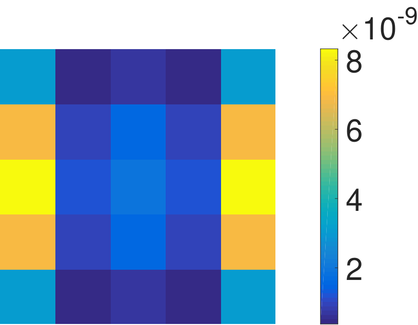
In this section, we consider a kernel similar to the one used in Section IV-B, which is displayed in the middle of Fig. 3 (the difference between the two kernels is shown in the right). Note that this trivial change implies that the Fourier transform of the new kernel has some values that are very close to zero, which may drastically impact the performance of the FUSE algorithm. The fusion performance of FUSE and R-FUSE with a TV prior is summarized in Table II. Obviously, the performance of FUSE degrades a lot due to the presence of close-to-zero values in the kernel FT, which does not agree with the invertibility assumption of ${\mathbf{D}}$. On the contrary, the proposed R-FUSE provides results very close to (almost the same with) those obtained in Section IV-B, demonstrating its robustness w.r.t. the blurring kernel.

References

- [1] Q. Wei, N. Dobigeon, and J.-Y. Tourneret, “Fast fusion of multi-band images based on solving a Sylvester equation,” IEEE Trans. Image Process., vol. 24, no. 11, pp. 4109–4121, Nov. 2015.
- [2] L. Loncan, L. B. Almeida, J. M. Bioucas-Dias, X. Briottet, J. Chanussot, N. Dobigeon, S. Fabre, W. Liao, G. Licciardi, M. Simoes, J.-Y. Tourneret, M. Veganzones, G. Vivone, Q. Wei, and N. Yokoya, “Hyperspectral pansharpening: a review,” IEEE Geosci. Remote Sens. Mag., vol. 3, no. 3, pp. 27–46, Sept. 2015.
- [3] C.-I. Chang, Hyperspectral data exploitation: theory and applications. New York: John Wiley & Sons, 2007.
- [4] H. Aanaes, J. Sveinsson, A. Nielsen, T. Bovith, and J. Benediktsson, “Model-based satellite image fusion,” IEEE Trans. Geosci. Remote Sens., vol. 46, no. 5, pp. 1336–1346, May 2008.
- [5] T. Stathaki, Image fusion: algorithms and applications. New York: Academic Press, 2011.
- [6] M. Gong, Z. Zhou, and J. Ma, “Change detection in synthetic aperture radar images based on image fusion and fuzzy clustering,” IEEE Trans. Image Process., vol. 21, no. 4, pp. 2141–2151, Apr. 2012.
- [7] A. P. James and B. V. Dasarathy, “Medical image fusion: A survey of the state of the art,” Information Fusion, vol. 19, pp. 4–19, 2014.
- [8] B. Aiazzi, L. Alparone, S. Baronti, A. Garzelli, and M. Selva, “25 years of pansharpening: a critical review and new developments,” in Signal and Image Processing for Remote Sensing, 2nd ed., C. H. Chen, Ed. Boca Raton, FL: CRC Press, 2011, ch. 28, pp. 533–548.
- [9] A. Gupta and D. Nagar, Matrix Variate Distributions, ser. Monographs and Surveys in Pure and Applied Mathematics. Taylor & Francis, 1999.
- [10] Q. Wei, N. Dobigeon, and J.-Y. Tourneret, “Bayesian fusion of multi-band images,” IEEE J. Sel. Topics Signal Process., vol. 9, no. 6, pp. 1117–1127, Sept. 2015.
- [11] ——, “Bayesian fusion of multispectral and hyperspectral images using a block coordinate descent method,” in Proc. IEEE GRSS Workshop Hyperspectral Image SIgnal Process.: Evolution in Remote Sens. (WHISPERS), Tokyo, Japan, Jun. 2015.
- [12] M. Simoes, J. Bioucas-Dias, L. Almeida, and J. Chanussot, “A convex formulation for hyperspectral image superresolution via subspace-based regularization,” IEEE Trans. Geosci. Remote Sens., vol. 53, no. 6, pp. 3373–3388, Jun. 2015.
- [13] Q. Wei, J. Bioucas-Dias, N. Dobigeon, and J. Tourneret, “Hyperspectral and multispectral image fusion based on a sparse representation,” IEEE Trans. Geosci. Remote Sens., vol. 53, no. 7, pp. 3658–3668, Jul. 2015.
- [14] M. Afonso, J. M. Bioucas-Dias, and M. Figueiredo, “An augmented Lagrangian approach to the constrained optimization formulation of imaging inverse problems.” IEEE Trans. Image Process., vol. 20, no. 3, pp. 681–95, 2011.
- [15] C.-I. Chang, X.-L. Zhao, M. L. Althouse, and J. J. Pan, “Least squares subspace projection approach to mixed pixel classification for hyperspectral images,” IEEE Trans. Geosci. Remote Sens., vol. 36, no. 3, pp. 898–912, 1998.
- [16] J. M. Bioucas-Dias and J. M. Nascimento, “Hyperspectral subspace identification,” IEEE Trans. Geosci. Remote Sens., vol. 46, no. 8, pp. 2435–2445, 2008.
- [17] R. H. Bartels and G. Stewart, “Solution of the matrix equation AX+ XB= C,” Communications of the ACM, vol. 15, no. 9, pp. 820–826, 1972.
- [18] M. A. Woodbury, “Inverting modified matrices,” Memorandum report, vol. 42, p. 106, 1950.
- [19] D. Fleming, “Effect of relative spectral response on multi-spectral measurements and NDVI from different remote sensing systems,” Ph.D. dissertation, University of Maryland, Department of Geography, USA, 2006.