Asymptotics of random domino tilings of rectangular Aztec diamonds

Alexey Bufetov Alexey BufetovDepartment of Mathematics, Massachusetts Institute of Technology, Cambridge, MA, USA. E-mail: alexey.bufetov@gmail.com and Alisa Knizel Alisa KnizelDepartment of Mathematics, Massachusetts Institute of Technology, Cambridge, MA, USA. E-mail: alisik@math.mit.edu

Abstract.

We consider asymptotics of a domino tiling model on a class of domains which we call rectangular Aztec diamonds. We prove the Law of Large Numbers for the corresponding height functions and provide explicit formulas for the limit. For a special class of examples, the explicit parametrization of the frozen boundary is given. It turns out to be an algebraic curve with very special properties. Moreover, we establish the convergence of the fluctuations of the height functions to the Gaussian Free Field in appropriate coordinates. Our main tool is a recently developed moment method for discrete particle systems.

1. Introduction

We study the asymptotic behavior of uniformly random domino tilings of domains drawn on the square grid. This model has received a significant attention in the last twenty five years ([16], [17], [20], [27], [29], [30]). Let us briefly describe our results.

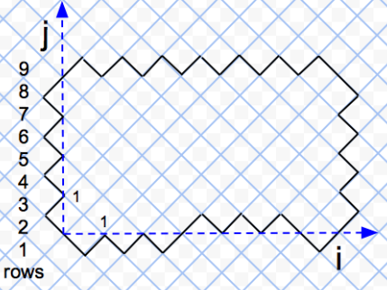
We consider a class of domains, which we call rectangular Aztec diamonds, see Figure 1 for an example. This type of domains generalizes a well-known case of the Aztec diamond, introduced in [20], at the same time inheriting many of its combinatorial properties. For instance, similar to the Aztec diamond, the domains we consider also have a rectangular shape with sawtooth boundary.

Refer to caption — Figure 1. Domino tiling of a Rectangular Aztec diamond $\mathcal{R}(6,(1,2,3,7,8,9),3)$ .

The main feature of this class of domains is a variety of different boundary conditions which are allowed on one side of the rectangle. These boundary conditions are parameterized by configurations of boxes with dots as presented in Figure 1. When the mesh size goes to zero the limit behavior of the boundary boxes can be parameterized by a probability measure ${\boldsymbol{\eta}}$ on $\mathbb{R}$ with a compact support. We are able to analyze a global asymptotic behavior of the uniform random tiling of such a domain for an arbitrary choice of this measure.

Limit shape. A domino tiling can be conveniently parameterized by the so-called height function, see Section 3.2. It is an integer-valued function on the vertices of the square grid inside the domain, which satisfies certain conditions (see Definition 3.10 for further details). There is a one-to-one correspondence between tilings and height functions (as long as the height is fixed at one vertex). A random domino tiling naturally gives rise to a random height function. In Theorem 3.12 we prove that for an arbitrary measure ${\boldsymbol{\eta}}$ a random height function converges to a deterministic function as the mesh size of the grid goes to zero, furthermore, we give an explicit formula for it.

In [17] it was shown that the limit shape exists for a wide class of domains on the square grid and can be found as a solution to a certain variational problem. Our approach is different and provides an explicit formula for the limit height function. Our computation of the limit shape is closely related to the notion of the free projection from the Free Probability Theory (see Remark 3.9).

Frozen boundary. Typically, a limit shape forms frozen facets, that is areas, where only one type of domino is present. There also exists a connected open liquid region inside the domain in which arbitrary local configurations of dominos are present. The curve, which separates the liquid region from the frozen zones is called frozen boundary.

In a particular case, when the measure ${\boldsymbol{\eta}}$ is a uniform measure of density $1$ on a union of $s$ segments such that their lengths add to $1$ , we give an explicit parametrization of the frozen boundary, see Theorem 5.1. It turns out to be an algebraic curve of rank $2s$ and genus zero with very special properties. The degree of the frozen boundary linearly depends on the number of segments. Therefore, the subclass of domains we consider provides a diverse variety of limit shapes of an arbitrary complexity.

Moreover, our formulas allow to analyze the frozen boundary for an arbitrary measure ${\boldsymbol{\eta}}$ . We discuss several examples in Section 7.

Fluctuations. For arbitrary boundary conditions on one side of the rectangular Aztec diamond we prove a Central Limit Theorem for a global behavior of the random height function (see Theorem 6.9), which is the main result of this paper. We show that after a suitable change of coordinates the fluctuations are described by the Gaussian Free Field. The appearance of the Gaussian Free Field as a universal object in this class of probabilistic tiling models originates from the work of Kenyon (see [30], [31] ).

In [30] Kenyon proved a central limit theorem for uniformly random tilings of domains of an arbitrary shape, but with very special boundary conditions such that the limit shape does not have any frozen facets. In contrast, we analyze rectangular domains with arbitrary boundary conditions on one of the sides and the limit shape in our case always has frozen facets. The fluctuations of the liquid region for a random tiling model containing both frozen facets and liquid region were first studied in [4].

Depending on the boundary conditions, the Law of Large Numbers can have a quite complicated form. It is reflected in a (possibly complicated) choice of the complex structure, that is a map from the liquid region into the complex half-plane. In other words, it is the choice of the coordinate in which the Gaussian Free Field appears as a limit object.

A parallel (and actually more developed) story exists for the case of lozenge tilings. We refer to [32] for the exposition and further references on the subject. Both the domains we consider and the fluctuation results are close in spirit to [39], [40], however, the approach we take is entirely different.

We use a moment method for this type of problems. It was introduced and developed in [9], [10]. Let us comment on two other known methods. The method based on the study of a family of orthogonal polynomials, which was extensively used in the case of the Aztec diamond, does not seem to be available in our setting. A large class of tiling problems fits the framework of Schur processes which was introduced in [38]. It was shown in [38] that any Schur process is a determinantal process with a correlation kernel suitable for asymptotics analysis. Papers [18],[39], [40] study the lozenge tiling model which is combinatorially similar to a Schur process yet does not fit this framework; a significant effort was necessary to derive a correlation kernel there. It is an important challenge to find a reasonable correlation kernel for the tiling model studied in the present paper and to perform its asymptotic analysis. However, we believe that the moment method is the most suitable method for the analysis of the global behavior in this class of problems (see Remark 6.10 for further comments).

In this paper we give a “model case” analysis of a specific class of domino tilings. However, we believe that the moment method and the tools developed in this paper are applicable in many other models. Let us mention some of them.

The domino tiling model considered in this paper can be interpreted as a random collection of non-intersecting lines, see Figure 4 and Section 2.3 for details. In the case of the Aztec diamond this interpretation was first used by Johansson in [28], and later many similar and more general ensembles of non-intersecting lines were studied, see [6], [5], [8], [7] and references therein. Some of these ensembles can be viewed as dimer models. More precisely, in [7] it was shown how to interpret an arbitrary Schur process as a dimer model on a so-called rail yard graph.

The main novelty of the presented approach is that we consider non-intersecting lines with arbitrary boundary conditions on one side. We suggest that all such models can be analyzed with the use of the moment method and the results of this paper. Because the global behavior of the height function significantly depends on the boundary conditions in all these models, we expect further interesting results in this direction.

This paper is organized as follows. In Section 2 we discuss combinatorial properties of rectangular Aztec diamonds. In Sections 3 and 4 we analyze the limit shape of the tilings. In Section 5 we study the frozen boundary for a specific class of examples. In Section 6 we prove the global Central Limit Theorem. In Section 7 we study some examples which are not covered by Section 5. In 8. Appendix A we briefly comment on a more general class of probability measures on rectangular Aztec diamonds. In 9. Appendix B we provide a result on the local behavior of these tilings.

Acknowledgements

The authors are deeply grateful to Alexei Borodin and Vadim Gorin for very helpful discussions. The authors would like to thank anonymous referees for many valuable comments which helped to improve the manuscript.

2. The model description

In this section we study the combinatorics of the model. We establish a bijection between the domino tilings of a rectangular Aztec diamond and the sequences of Young diagrams with some special properties. This will allow us to bring in the machinery of the Schur functions to study the asymptotics. The key observation is Proposition 2.13.

In the end of the section we discuss another combinatorial realization for our model through the non-intersecting line ensembles, which was mentioned in introduction.

2.1. Combinatorics of the model

Let us present a formal definition of the domain we are considering.

Definition 2.1.

Let $N\in\mathbb{N}$ and $\Omega=(\Omega_{1},\dots,\Omega_{N})$ , where $1=\Omega_{1}<\Omega_{2}<\dots<\Omega_{N}$ and $\Omega_{i}\in\mathbb{N}$ . Set $m=\Omega_{N}-N.$

Introduce the coordinates $(i,j)$ as in Figure 5. Let us denote by $C(i,j)$ a unit square with the vertex coordinates $(i,j),$ $(i-\frac{1}{2},j+\frac{1}{2}),$ $(i+\frac{1}{2},j+\frac{1}{2}),$ $(i,j+1).$

The rectangular Aztec diamond $\mathcal{R}(N,\Omega,m)$ is a polygonal domain which is built of $2N+1$ rows of unit squares $C(i,j).$ Let us enumerate the rows starting from the bottom as shown in Figure 5. Then the $k$ -th row consists of unit squares $C(i,j),$ where

•

$i=0,1,\dots,\Omega_{N}$ and $j=0,1,\dots,N-1,$ when $k=2s,$ $s=0,1,\dots,N;$
•

$i=\frac{1}{2},\frac{3}{2},\dots,\Omega_{N}-\frac{1}{2}$ and $j=\frac{1}{2},\frac{3}{2},\dots,N-\frac{1}{2},$ when $k=2s+1,$ $s=1,2,\dots,N;$
•

$i=\Omega_{l}-\frac{1}{2}$ and $j=-\frac{1}{2}$ for $l=1,2,\dots,N,$ when $k=1.$ We call this row the boundary of $\mathcal{R}(N,\Omega,m)$ .

Definition 2.2.

A domino tiling of a rectangular Aztec diamond $\mathcal{R}(N,\Omega,m)$ is a set of pairs $(C(i_{1},j_{1}),C(i_{2},j_{2})),$ called dominos, such that the unit squares $C(i_{1},j_{1}),C(i_{2},j_{2})\subset\mathcal{R}(N,\Omega,m)$ share an edge and every unit square belongs to exactly one domino.

Let us denote the set of domino tilings of $\mathcal{R}(N,\Omega,m)$ by $\mathfrak{D}(N,\Omega,m).$

Definition 2.3.

Let $D\in\mathfrak{D}(N,\Omega,m)$ be a domino tiling of $\mathcal{R}(N,\Omega,m).$ We call a domino $d=(C(i_{1},j_{1}),C(i_{2},j_{2}))\in D$ a $V$ -domino if $max(i_{1},i_{2})\in\mathbb{N}$ and we call it a $\Lambda$ -domino otherwise. In other words, the dominos going upwards starting from an odd row are $V$ -dominos and those ones starting from an even row are $\Lambda$ -dominos. We also call the corresponding squares $C(i_{1},j_{1}),C(i_{2},j_{2})$ — $V$ -squares and $\Lambda$ -squares accordingly.

Lemma 2.4.

The set of V-squares in $\mathcal{R}(N,\Omega,m)$ determines the tiling uniquely.

Proof.

Let us reconstruct the tiling given the set of V-squares coming from some unknown tiling. We will show that we can reconstruct it in a unique way. Let us enumerate the squares in each row from left to right.

We start by looking at the V-squares in the first row. All squares in the first row are V-squares and there are exactly $N$ of them. Let us take the first V-square in the first row. We will pair it with the first V-square in the second row. We can always do it since we know that there exists at least one domino tiling with this set of V-squares. We can proceed until the end of the first row. Note that at this point we have used all V-squares from the second row and this is the only way we could pair the V-squares from the first row with something.

Now we pair the first $\Lambda$ -square in the second row with the first $\Lambda$ -square in the third row. We can proceed until the end of the second row. Note that at this point we have used all squares from the second row and all $\Lambda$ -squares from the third row. Moreover, this is the only way we could pair $\Lambda$ -squares from the second row with something. Now we look at V-squares in the third row and notice that there are $N-1$ of them. This is because the total number of squares in the third row is less by one than the total number of squares in the second row. We start pairing them with V-squares from the third row in the same way.

We continue in this fashion until we pair all $\Lambda$ -squares from row $2N$ with all the squares from row $2N+1.$

∎

Definition 2.5.

Let $\mu$ be a $n$ -tuple of natural numbers $\mu=(\mu_{1}\geq\mu_{2}\dots\geq\mu_{n}\geq 0).$ We will denote $\ell(\mu)=n.$ A Young diagram $Y_{\mu}$ is a set of boxes in the plane with $\mu_{1}$ boxes in the first row, $\mu_{2}$ boxes in the second row, etc.

We call a Young diagram $Y_{\mu}$ rectangular $n\times m$ Young diagram if $m=\mu_{1}=\mu_{2}=\dots=\mu_{n}.$ Let us denote it $Y_{n\times m}.$

Definition 2.6.

Let $Y_{\mu}$ be a Young diagram, where $\mu=\mu_{1}\geq\mu_{2}\dots\geq\mu_{n}\geq 0.$ A dual Young diagram $Y_{\mu^{\vee}}$ is obtained by taking the transpose of the original diagram $Y_{\mu}$ . Explicitly we have that $\mu^{\vee}_{i}$ is equal to the length of the $i$ -th column of $Y_{\mu}.$

Construction 2.7.

Due to Lemma 2.4 we can encode any domino tiling $D\in\mathfrak{D}(N,\Omega,m)$ pictorially as it is shown in Figure $\ref{fig:points}.$ We simply put a yellow node in the center of every V-square from an even row and a pink node in the center of every V-square from an odd row. The configuration of these nodes determines the tiling uniquely. In the case of the Aztec diamond such encoding was suggested by Johansson [28].

Let us associate to every configuration of the nodes the following sequence of Young diagrams $Y_{j}$ . Each diagram $Y_{j}$ corresponds to the $j$ -th row $j=1,2,\dots,2N$ , which has $n_{j}$ V-squares and $m_{j}$ $\Lambda$ -squares. Let us take a rectangular $n_{j}\times m_{j}$ Young diagram. We start drawing a stepped line $\ell_{j}$ inside it starting from the left bottom corner. At step $k$ if the $i$ -th square in the row is a V-square $\ell_{j}$ goes up by one, otherwise the line goes to the right by one. The stepped line $\ell_{j}$ is the boundary of a Young diagram, see Figure $\ref{fig:diagram}.$

Let us look at the $j$ -th row. It has $N-\lfloor\frac{j-1}{2}\rfloor$ V-squares in positions $i_{1},\dots,i_{N-\lfloor\frac{j-1}{2}\rfloor}$ starting from the left. Then the Young diagram we obtain corresponds to the $N-\lfloor\frac{j-1}{2}\rfloor$ -tuple $(i_{N-\lfloor\frac{j-1}{2}\rfloor}-\lfloor\frac{j-1}{2}\rfloor,\dots,i_{2}-2,i_{1}-1).$

To construct a Young diagram corresponding to the boundary row we complete the row by virtually adding $m$ $\Lambda$ -squares so that $\mathcal{R}(N,\Omega,m)$ becomes a proper rectangular with sawtooth boundary. Let us denote the Young diagram corresponding to the boundary row $Y_{\omega},$ where $\omega$ is an $N$ -tuple of integers, more precisely, $\omega=(\Omega_{N}-N,\dots,\Omega_{1}-1).$

Definition 2.8.

Let $Y_{\omega}$ , where $\omega=\omega_{1}\geq\omega_{2}\dots\geq\omega_{N}\geq 0,$ be a Young diagram contained in a rectangle $N\times m$ Young diagram $Y_{N\times m}$ . Let $\mathcal{S}(Y,N,m)$ be the following set of sequences of Young diagrams

\mathcal{S}(Y_{\mu},N,m)=\{(Y_{\mu^{(N)}}=Y_{\omega},Y_{\nu^{(N)}},\dots,Y_{\mu^{(1)}},Y_{\nu^{(1)}}\},

such that

•

$\ell(\mu^{(i)})=i$ and $\ell(\nu^{(i)})=i$ for $i=1,2,\dots,N.$
•

$Y_{\mu^{(i)}}\subset Y_{i\times(m+N-i)}$ for $i=1,2,\dots,N;$
•

$Y_{\nu^{(i)}}\subset Y_{i\times(m+N-i+1)}$ for $i=1,2,\dots,N;$
•

$Y_{\mu^{(i)}}\subset Y_{\nu^{(i)}}$ for $i=1,2,\dots,N;$
•

$Y_{\nu^{(i)}}$ $\setminus$ $Y_{\mu^{(i)}}$ is a vertical strip of length $l\leq i$ for $i=1,2,\dots,N;$ that is $Y_{\nu^{(i)}}$ can be obtained from $Y_{\mu^{(i)}}$ by adding $l$ boxes, no two in the same row, see Figure 9.

•

$Y_{\nu^{(i+1)}}\setminus Y_{\mu^{(i)}}$ is a horizontal strip. In other words, they interlace $(Y_{\mu^{(i)}}\prec Y_{\nu^{(i+1)}}),$ that is

\nu^{(i+1)}_{1}\geq\mu^{(i)}_{1}\geq\dots\geq\nu^{(i+1)}_{i}\geq\mu^{(i)}_{i}\geq\nu^{(i+1)}_{i+1},\text{ for }i=1,2,\dots,N-1.

Theorem 2.9.

Construction 2.7 defines a map

Y\colon\mathfrak{D}(N,\Omega,m)\rightarrow\mathcal{S}(Y_{\omega},N,m).

The map is bijective.

Proof.

Let $\mathcal{D}\in\mathfrak{D}(N,\Omega,m)$ be a domino tiling and let $Y(\mathcal{D})=(Y_{\mu^{(n)}=\omega},Y_{\nu^{(N)}},\dots,Y_{\mu^{(1)}},Y_{\nu^{(1)}})$ . Let us first check that this map is well-defined, i.e. $Y(\mathcal{D})\in\mathcal{S}(Y_{\omega},N,m).$ Thus, we need to verify all the properties in Definition 2.8. Figure 10 illustrates the proof.

By construction $Y_{\mu^{(i)}}\subset Y_{n_{i}\times m_{i}},$ where $n_{i}$ and $m_{i}$ are the number of $V$ -squares and $\Lambda$ -squares in the row with number $2(N-i)+1$ . Following the proof of Lemma 2.4 we see that $n_{i}=i$ and $m_{i}=N+m-i.$ Also, the length of $Y_{\mu^{(i)}}$ is equal to the number of $V$ -squares in the corresponding row. Thus, we get $\ell(\mu^{(i)})=i.$ Similarly we have $Y_{\nu^{(i)}}\subset Y_{i\times(m+N-i+1)}$ and $\ell(\nu^{(i)})=i.$

Note that by construction $\mu_{j}^{(i)}$ is precisely the number of $\Lambda$ -squares to the left from the $j$ -th $V$ -square in the corresponding row with number $k=2(N-i)+1$ . Let us look at this row. The $V$ -squares from it are paired with $V$ -squares from the next row in $\mathcal{D}$ . It can be shown by induction that the number of $\Lambda$ -squares to the left from the $j$ -th $V$ -square in the $k+1$ row is always equal or greater by one than the same quantity for the $j$ -th $V$ -square in the $k$ -th row. It follows from the fact that if the $j$ -th $V$ -square is in position $n$ in the $k$ -th row (i.e. it is the $n$ -th square from the left in this row) it must be paired with the $j$ -th $V$ -square from the next row in position $n$ or $n+1,$ see Figure 6. Therefore, $Y_{\mu_{j}^{(i)}}\subset Y_{\nu_{j}^{(i)}}$ and $Y_{\nu^{(i)}}$ $\setminus$ $Y_{\mu^{(i)}}$ is a vertical strip with a number of blocks $\leq i.$

Consider $Y_{\nu^{\vee,(i)}},$ the Young diagram dual to $Y_{\nu^{(i)}}.$ Note that by construction $\nu^{\vee,(i)}_{j}$ is precisely the number of $V$ -squares to the left from the $j$ -th $\Lambda$ -square in the corresponding row with number $k=2(N-i)+2$ , where this time we count from the right. Let us look at this row. Then the $\Lambda$ -squares from the next row are paired with the $\Lambda$ -squares from this row, moreover, the $j$ -th $\Lambda$ -square in position $n$ is paired with the $j$ -th $\Lambda$ -square in position $n$ or $n+1$ from the next row counting from the right. Again, we get that $Y_{\nu^{\vee,(i)}}$ $\setminus$ $Y_{\mu^{\vee,(i+1)}}$ is a vertical strip. Thus, $Y_{\mu^{(i+1)}}$ $\setminus$ $Y_{\nu^{(i)}}$ is a horizontal strip. Therefore, the interlacing condition holds.

So far we have checked that the map $Y$ is well-defined. From Lemma 2.4 it follows that it is injective.

Let us construct the inverse map $Y^{(-1)}\colon\mathcal{S}(Y_{\alpha},N,m)\rightarrow\mathfrak{D}(N,\Omega,m).$ Inverting the Construction 2.7 we see that each element $y\in\mathcal{S}(Y_{\alpha},N,m)$ defines a configuration of V-squares. Our goal is to show that there exists a tiling with such a configuration of V-squares. We can reconstruct it using the same ideas as we used in the proof of Lemma 2.4. We start by pairing V-squares from the first row with V-squares from the second row starting from the left. We can always pair the $j$ -th V-square from the first row in position $n$ with the $i$ -th V-square from the second row because it has to be in position $n$ or $n+1$ due to our assumptions on $y.$ Then we proceed to the next row and pair $\Lambda$ -squares with $\Lambda$ squares in the third row. The map $Y^{(-1)}$ is then well-defined and injective. Therefore, $Y$ is a bijection. ∎

2.2. Uniform measure on $\mathcal{S}(Y_{\alpha},N,m)$ .

Theorem 2.9 allows us to reduce any question about the uniform measure on the set of domino tilings $\mathfrak{D}(N,\Omega,m)$ to the same question for the uniform measure on $\mathcal{S}(Y_{\alpha},N,m).$ This is the core of our approach.

Let $U(N)$ denote the group of all $N\times N$ complex unitary matrices. It is well-known that all irreducible representations of $U(N)$ are parameterized by their highest weights, which are signatures of length $N,$ that is, $N$ -tuples of integers $\lambda=(\lambda_{1}\geq\lambda_{2}\geq\dots\geq\lambda_{N}).$ We denote by $\mathbb{GT}_{N}$ the set of all signatures and the length of a signature is denoted by $\ell(\lambda)$ . We call a signature non-negative if $\lambda_{N}\geq 0.$ Note that the set of all nonnegative signatures $\mathbb{GT}_{N}^{+}$ is in bijection with the set of Young diagrams $\mathbb{Y}_{N}$ with $N$ rows (rows are allowed to have zero length).

Definition 2.10.

Let $\lambda\in\mathbb{GT}_{N}.$ The rational Schur function is

(2.1)

s_{\lambda}(u_{1},\dots,u_{N})=\frac{\textup{det}_{i,j=1,\dots,N}(u^{\lambda_{j}+N-j}_{i})}{\prod\limits_{1\leq i<j\leq N}(u_{i}-u_{j})}.

Proposition 2.11.

$($ Weyl, [45] $)$ The value of the character of the irreducible representation $\pi^{\lambda}$ corresponding to the signature $\lambda=(\lambda_{1}\geq\dots\geq\lambda_{N})$ on a unitary matrix $\mathfrak{u}\in U(N)$ with eigenvalues $u_{1},\dots,u_{n}$ is given by the rational Schur function:

\textup{Trace}(\pi^{\lambda}(\mathfrak{u}))=s_{\lambda}(u_{1},\dots,u_{N}).

Let $\mu^{(n)}$ and $\nu^{(n)}$ be two non-negative signatures of length $n.$ Recall that Schur functions form a basis for the algebra of symmetric functions. Define the coefficients $\mathrm{st}(\mu^{(n)}\rightarrow\nu^{(n)})$ and $\mathrm{pr}(\nu^{(n)}\rightarrow\mu^{(n-1)})$ via

(2.2)

\frac{s_{\mu^{(n)}}(u_{1},\dots,u_{n})}{s_{\mu^{(n)}}(1^{n})}\displaystyle\prod\limits^{n}_{i=1}\frac{(1+u_{i})}{2}=\sum_{\nu^{(n)}\in\mathbb{GT}_{n}}\mathrm{st}(\mu^{(n)}\rightarrow\nu^{(n)})\frac{s_{\nu^{(n)}}(u_{1},\dots,u_{n})}{s_{\nu^{(n)}}(1^{n})},

(2.3)

\frac{s_{\nu^{(n)}}(u_{1},\dots,u_{n-1},1)}{s_{\nu^{(n)}}(1^{n})}=\sum_{\mu^{(n-1)}\in\mathbb{GT}_{n-1}}\mathrm{pr}(\nu^{(n)}\rightarrow\mu^{(n-1)})\frac{s_{\mu^{(n-1)}}(u_{1},\dots,u_{n-1})}{s_{\mu^{(n-1)}}(1^{n})},

where $1^{n}$ is a notation for a string $(1,1,\dots,1)$ of length $n.$

Lemma 2.12.

The following equalities hold

(2.4)

\mathrm{st}(\mu^{(n)}\rightarrow\nu^{(n)})=\begin{cases}\frac{s_{\nu^{(n)}}(1^{n})}{2^{n}s_{\mu^{(n)}}(1^{n})},&\mu^{(n)}\subset\nu^{(n)};\\ 0,&{otherwise},\end{cases}

(2.5)

\mathrm{pr}(\nu^{(n)}\rightarrow\mu^{(n-1)})=\begin{cases}\frac{s_{\mu^{(n)}}(1^{n})}{s_{\nu^{(n)}}(1^{n})},&\mu^{(n-1)}\prec\nu^{(n)};\\ 0,&{otherwise.}\end{cases}

As a consequence,

(2.6)

\sum\limits_{\nu^{(n)}\in\mathbb{GT}_{n}}\mathrm{st}(\mu^{(n)}\rightarrow\nu^{(n)})=1\text{ and }\sum\limits_{\mu^{(n-1)}\in\mathbb{GT}_{n-1}}\mathrm{pr}(\nu^{(n)}\rightarrow\mu^{(n-1)})=1.

Proof.

Let us start with the first identity. Let $e_{l}$ be the $l$ -th elementary symmetric function. Recall the Pieri’s rule

e_{l}s_{\mu}=\sum\limits_{\mu\subset\lambda}s_{\lambda},

where the sum is taken over $\lambda$ obtained from $\mu$ by adding $l$ boxes, no two in the same row.

Note that

\displaystyle\prod\limits_{j=1}^{n}\frac{(1+u_{j})}{2}=\frac{1}{2^{n}}\sum\limits_{j=1}^{n}e_{j}(u_{1},\dots,u_{n}).

Therefore,

\mathrm{st}(\mu^{(n)}\rightarrow\nu^{(n)})=\begin{cases}\frac{s_{\nu^{(n)}}(1^{n})}{2^{n}s_{\mu^{(n)}}(1^{n})},&\mu^{(n)}\subset\nu^{(n)};\\ 0,&{otherwise},\end{cases}

where $\nu^{(n)}$ is obtained from $\mu^{(n)}$ by adding $l$ boxes such that $l\leq n.$

We can also compute

(2.7)

s_{\mu^{(n)}}(1^{n})e_{l}(1^{n})=s_{\mu^{(n)}}(1^{n})\binom{n}{l}=\sum\limits_{\mu^{(n)}\subset\lambda}s_{\lambda}(1^{n}),

where the sum is taken over $\lambda$ obtained from $\mu^{(n)}$ by adding $l$ boxes, no two in the same row.

From (2.7) we conclude

\sum\limits_{\nu^{(n)}\in\mathbb{GT}_{n}}\mathrm{st}(\mu^{(n)}\rightarrow\nu^{(n)})=\frac{1}{2^{n}}\sum\limits_{l=1}^{n}\binom{n}{l}=1.

The equation (2.3) is a well-known branching rule for the Schur polynomials. Thus, we get

\mathrm{pr}(\nu^{(n)}\rightarrow\mu^{(n-1)})=\begin{cases}\frac{s_{\mu^{(n)}}(1^{n})}{s_{\nu^{(n)}}(1^{n})},&\mu^{(n-1)}\prec\nu^{(n)};\\ 0,&{otherwise.}\end{cases}

Moreover, we have

\textup{dim}(\pi^{\mu^{(n)}})=s_{\mu^{(n)}}(1^{n})=\sum\limits_{\nu^{(n)}\prec\mu^{(n)}}\textup{dim}(\pi^{\nu^{(n)}})=\sum\limits_{\nu^{(n)}\prec\mu^{(n)}}s_{\nu^{(n)}}(1^{n}).

∎

Let us fix a signature $\mu$ of length $N.$ Lemma 2.12 allows us to define a probability measure on the sequences of signatures of the form

\mathcal{S}^{N}=\{(\mu^{(N)},\nu^{(N)},\dots,\mu^{(1)},\nu^{(1)})\}

by the formula

(2.8)

\mathcal{P}^{N}_{\mu}\left((\mu^{(N)},\nu^{(N)},\dots,\mu^{(1)},\nu^{(1)})\right)=\\ =1_{\mu^{(N)}=\mu}\mathrm{st}(\mu^{(N)}\rightarrow\nu^{(N)})\prod\limits_{j=1}^{N-1}\mathrm{pr}(\nu^{(N-j+1)}\rightarrow\mu^{(N-j)})\mathrm{st}(\mu^{(N-j)}\rightarrow\nu^{(N-j)}),

where $\mu^{(i)},\nu^{(i)}\in\mathbb{GT}_{i}.$

This measure is similar to a Schur process; the only difference is that we fix a boundary condition $\mu$ (the factor $1_{\mu^{(N)}}=\mu$ in the formula (2.8)) which does not fit the framework of Schur processes (boundary conditions have to be empty there). It is this difference that significantly distinguishes asymptotic analysis of our model (as well as models in [18], [39], [40]) with the case of Schur processes.

Proposition 2.13.

Let $\mathcal{R}(\Omega,N,m)$ be a rectangular Aztec diamond. Let us denote the support of measure $\mathcal{P}^{N}_{\omega}$ by $\mathbb{S}_{\omega},$ where $\omega$ is the signature corresponding to the boundary row of $\mathcal{R}(\Omega,N,m).$ The set of domino tilings $\mathfrak{D}(\Omega,N,m)$ of $\mathcal{R}(\Omega,N,m)$ is in bijection with $\mathbb{S}_{\omega}.$ Moreover, the measure $\mathcal{P}^{N}_{\omega}$ is uniform on $\mathbb{S}_{\omega}$ and, therefore, on $\mathfrak{D}(\Omega,N,m).$

Proof.

From (2.5) and (2.4) for any $(\mu^{(N)},\nu^{(N)},\dots,\mu^{(1)},\nu^{(1)})$ we have

		$\displaystyle\mathcal{P}^{N}_{\omega}\left((\mu^{(N)},\nu^{(N)},\dots,\mu^{(1)},\nu^{(1)})\right)=$
		$\displaystyle=\frac{1}{2^{N}}\frac{s_{\nu^{(1)}}(1^{N})}{s_{\mu^{(1)}}(1^{N})}\frac{s_{\mu^{(2)}}(1^{N-1})}{s_{\nu^{(1)}}(1^{N})}\frac{1}{2^{N-1}}\frac{s_{\nu^{(2)}}(1^{N-1})}{s_{\mu^{(2)}}(1^{N-1})}\cdots\frac{1}{2}\frac{s^{\nu^{(N)}}(1)}{s_{\mu^{(N)}}(1)}=$
		$\displaystyle=\frac{1}{2^{N(N+1)/2}s_{\omega}(1^{N})},$

when $(\mu^{(N)},\nu^{(N)},\dots,\mu^{(1)},\nu^{(1)})\in\mathcal{S}(Y_{\omega},N,m)$ and zero otherwise. Recall that by Theorem 2.9 the set $\mathcal{S}(Y_{\omega},N,m)$ is in bijection with the set of domino tilings $\mathfrak{D}(\Omega,N,m).$

Therefore, $\mathcal{P}^{N}_{\omega}$ defines the uniform measure on $\mathfrak{D}(\Omega,N,m).$

∎

Corollary 2.14.

The number of domino tilings of $\mathcal{R}(\Omega,N,m)$ is equal to

(2.9)

|\mathfrak{D}(\Omega,N,m)|=2^{N(N+1)/2}s_{\omega}(1^{N}).

This formula was obtained in [15] based on the results from [14] and [35], see also [26]. There are many ways to prove the corresponding formula in the case of the Aztec diamond, see [20].

2.3. Non-intersecting line ensembles

Let us describe in more detail another combinatorial interpretation of our tiling model, which was discussed in the introduction.

One can imagine superimposing a rectangular Aztec diamond upon a checkerboard coloring and obtaining four types of dominos, as the black unit square might be either to the right/left (resp. top/bottom) unit square of a horizontal (resp. vertical) domino. In this way to each tiling one can bijectively associate a set of non-intersecting lines, as shown in Figure 4. This construction first appeared in [28], we use a slightly different but equivalent representation from [5].

Next, one can think of a rectangular Aztec diamond as being embedded into tilings of $\mathbb{R}^{2}$ , where outside the domain we add only non-overlapping horizontal dominos and fill the whole space with them. Then, by means of a simple transformation one obtains a bijection between a tiling of a rectangular Aztec diamond $\mathcal{R}(N,\Omega,m)$ and a configuration of non-intersecting lines on a Lindström-Gessel-Viennot (LGV) directed graph (see [21] and [42]), built out of $N+m$ basic blocks, see Figure 11. Note that $\Omega$ determines the boundary conditions along the bottoms of the basic blocks as shown in Figure 11. By construction from a yellow vertex a line can go up-right or to the right, while from a red vertex the line goes to the right or down-right.

Introduce the coordinate system as in the right picture in Figure 11. Let us associate to every vertical section $t=i,$ where $i=1,\dots 2N+1,$ a signature. Consider the set of nodes on a section. Suppose the nodes that belong to the lines from the ensemble have coordinates $s_{1}>s_{2}>\dots>s_{i}.$ Then the corresponding signature is $(s_{1}+1\geq s_{2}+2\geq\dots\geq s_{i}+i).$ In this way to every non-intersecting line ensemble one associates a sequence of signatures $(\gamma_{1},\rho_{1},\dots,\gamma_{N},\rho_{N},\gamma_{N+1}).$ Note that $\gamma_{N+1}=(0\geq 0\geq\dots\geq 0).$

Consider the following probability model on the set of the non-intersecting line ensembles. Let us assign weight $1$ to each horizontal edge, weight $\alpha=1$ to each vertical edge and $\beta=\frac{1}{2}$ to each down-right edge. Consider the $i$ -th basic block, let $(\gamma_{i},\rho_{i},\gamma_{i+1})$ be a triple of signatures corresponding to its left side, middle section and its right side. Let us assign to this block the following weight

w(\text{block})=s_{\rho_{i}/\gamma_{i+1}}(\alpha)\cdot s_{\rho_{i}/\gamma_{i}}(\hat{\beta}),

where $s_{\rho/\gamma}$ is a skew Schur function. Here $\alpha$ stands for the specialization of the symmetric functions into a single nonzero variable equal to $\alpha$ (with complete homogeneous symmetric functions specializing into $h_{n}(\alpha)=\alpha^{n},n\geq 0)$ , and $\hat{\beta}$ stands for the specialization into a single “dual” variable equal to $\beta$ (with complete homogeneous symmetric functions specializing into $h_{n}(\hat{\beta})=1$ if $n=0,$ $h_{n}(\hat{\beta})=\beta$ if $n=1$ , and $h_{n}(\hat{\beta})=0$ if $n\geq 2)$ . The quantities $w(\text{block})$ are essentially indicators times a power of a parameter.

Define the probability $\mathbb{P}_{L}$ of an non-intersecting line ensemble satisfying our combinatorial and boundary conditions to be the product of the corresponding weights of the blocks.

Proposition 2.15.

Measure $\mathbb{P}_{L}$ is a uniform probability measure on the set $L(N,\Omega,m)$ of all non-intersecting line ensembles satisfying our combinatorial and boundary conditions.

We do not go into details of the proof of this proposition since we will not need it further, see the recent exposition in [2].

We conclude that the uniform measure on the set of tilings $\mathfrak{D}(N,\Omega,m)$ corresponds under the above bijection to a measure $\mathbb{P}_{L}$ on the ensembles of non-intersecting lines.

There are many other interesting tiling models that have an interpretation as ensembles of non-intersecting lines. For example, random tilings of a tower, discussed in [5]. More generally, the random dimer model on a rail yard graph [7] fits into the framework of the Schur generating functions. We believe that our approach can be used to analyze the global behavior for these models with arbitrary boundary conditions.

3. Law of Large numbers

The main technique we use in the paper is the moment method introduced by Bufetov and Gorin in [9] and [10]. In this section we first present some background to give an overview of the method and then show that the model of random domino tilings of rectangular Aztec diamonds fits into this framework. Subsequently, we prove the Law of Large numbers for the random height function.

3.1. LLN for the moments

One way to encode a signature $\lambda\in\mathbb{GT}_{N}$ is through the counting measure $m[\lambda]$ on $\mathbb{R}$ corresponding to it via

(3.1)

m[\lambda]=\frac{1}{N}\sum_{i=1}^{N}\delta\left(\frac{\lambda_{i}+N-i}{N}\right),

where $\delta$ is a delta measure. Note that we incorporate the scaling into this formula.

Let $\rho$ be a probability measure on the set of all signatures $\mathbb{GT}_{N}.$ The pushforward of $\rho$ with respect to the map $\lambda\rightarrow m[\lambda]$ defines a random probability measure on $\mathbb{R}$ that we denote $m[\rho].$

Definition 3.1.

Let $\rho$ be a probability measure on $\mathbb{GT}_{N}.$ The Schur generating function $\mathcal{S}^{U(N)}_{\rho}(u_{1},\dots,u_{N})$ is a symmetric Laurent power series in $(u_{1},\dots,u_{N})$ given by

(3.2)

\mathcal{S}^{U(N)}_{\rho}(u_{1},\dots,u_{N})=\sum\limits_{\lambda\in\mathbb{GT}(N)}\rho(\lambda)\frac{s_{\lambda}(u_{1},\dots,u_{N})}{s_{\lambda}(1,\dots,1)}.

We will need the following two results from [9].

Theorem 3.2.

$($ [9], Theorem 5.1 $)$ Let $\rho(N)$ be a sequence of measures such that for each $N=1,2,\dots$ , $\rho(N)$ is a probability measure on $\mathbb{GT}_{N}$ . Suppose that $\rho(N)$ is such that for every $j$

\lim_{N\to\infty}\frac{1}{N}\ln(\mathcal{S}^{U(N)}_{\rho(N)}(u_{1},\dots,u_{j},1^{N-j}))=Q(u_{1})+\dots+Q(u_{j}),

where $Q$ is an analytic function in a neighborhood of $1$ and the convergence is uniform in an open $($ complex $)$ neighborhood of $(1,\dots,1)$ . Then random measures $m[\rho(N)]$ converge as $N\to\infty$ in probability, in the sense of moments to a deterministic measure ${\boldsymbol{\eta}}$ on $\mathbb{R}$ , whose moments are given by

(3.3)

\int_{\mathbb{R}}x^{j}{\boldsymbol{\eta}}(dx)=\sum_{\ell=0}^{j}\frac{j!}{\ell!(\ell+1)!(j-\ell)!}\frac{\partial^{\ell}}{\partial u^{\ell}}\left(u^{j}Q^{\prime}(u)^{j-l}\right)\Biggr|_{u=1}.

Let us introduce some notation. Let $\eta$ be a compactly supported measure on $\mathbb{R}.$ Let $M_{k}({\boldsymbol{\eta}})=\int_{\mathbb{R}}x^{k}{\boldsymbol{\eta}}(dx)$ be its $k$ -th moment. Set

(3.4)

S_{\eta}(z)=z+M_{1}({\boldsymbol{\eta}})z^{2}+z^{3}M_{2}({\boldsymbol{\eta}})+\dots

to be the generating function of the moments of $\eta.$ Define $S_{\eta}^{(-1)}(z)$ to be the inverse series to $S_{\eta}(z)$ , that is $S_{\eta}^{(-1)}\bigl(S_{\eta}(z)\bigr)=S_{\eta}\bigl(S_{\eta}^{(-1)}(z)\bigr)=z.$

Let

(3.5)

R_{\eta}(z)=\frac{1}{S_{\eta}^{(-1)}(z)}-\frac{1}{z}

be the Voiculescu $R$ –transform of measure $\eta.$

Define the function $\textup{H}_{\eta}(u)$ as

(3.6)

\textup{H}_{\eta}(u)=\int_{0}^{\ln(u)}R_{\eta}(t)dt+\ln\left(\frac{\ln(u)}{u-1}\right),

which should be understood as a power series in $(u-1)$ .

Note that we have the following expression for its derivative:

(3.7)

\textup{H}^{\prime}_{\eta}(u)=\frac{1}{uS_{\eta}^{(-1)}(\log u)}-\frac{1}{u-1}.

Lemma 3.3.

If $\eta$ is a measure with compact support, then $\textup{H}_{\eta}(u)$ as a power series in $(u-1)$ is uniformly convergent in an open neighborhood of $u=1$ .

Proof.

Immediately follows from the definitions. ∎

We will need the following mild technical assumption.

Definition 3.4.

A sequence of signatures $\lambda(N)\in\mathbb{GT}_{N}$ is called regular, if there exists a piecewise–continuous function $f(t)$ and a constant $C$ such that

(3.8)

\lim_{N\to\infty}\frac{1}{N}\sum_{j=1}^{N}\left|\frac{\lambda_{j}(N)}{N}-f(j/N)\right|=0

and

(3.9)

\left|\frac{\lambda_{j}(N)}{N}-f(j/N)\right|<C,\quad\quad j=1,\dots,N,\quad N=1,2,\dots.

Remark 3.5.

Informally, the condition (3.8) means that scaled by $N$ coordinates of $\lambda(N)$ approach a limit profile $f$ . The restriction that $f(t)$ is piecewise–continuous is reasonable, since $f(t)$ is a limit of monotone functions and, thus, is monotone $($ therefore, we only exclude the case of countably many points of discontinuity for $f$ $)$ . We use condition (3.9) since it guarantees that all the measures which we assign to signatures and their limits have $($ uniformly $)$ compact supports — thus, these measures are uniquely defined by their moments.

Theorem 3.6.

$($ [9], [24],[25] $)$ Suppose that $\lambda(N)\in\mathbb{GT}_{N}$ , $N=1,2,\dots$ is a regular sequence of signatures, such that $\lim_{N\to\infty}m[\lambda(N)]={\boldsymbol{\eta}}\text{ (in weak topology)}.$ Then for any $j=1,2,\dots,N$ we have

(3.10)

\lim_{N\to\infty}\frac{1}{N}\ln\left(\frac{s_{\lambda(N)}(u_{1},\dots,u_{j},1^{N-j})}{s_{\lambda(N)}(1^{N})}\right)=\textup{H}_{\boldsymbol{\eta}}(u_{1})+\dots+\textup{H}_{\boldsymbol{\eta}}(u_{j}),

where the convergence is uniform over an open $($ complex $)$ neighborhood of $(1,\dots,1).$

The uniform measure on the set of domino tilings of a rectangular Aztec diamond $\mathcal{R}(N,\Omega,m)$ induces a measure on the set of all possible configurations of $N-\lfloor\frac{k-1}{2}\rfloor$ $V$ -squares in the $k$ -th row, for $k=1,\dots,2N.$ Due to Theorem 2.13 we can think of it from the other prospective, more precisely, as a measure on the signatures $\lambda\in\mathbb{GT}_{N-\lfloor\frac{k-1}{2}\rfloor}.$ Let us denote the measure we get on the set of signatures by $\rho^{k}(N)$ and $\lfloor\frac{k-1}{2}\rfloor$ by $t.$

Lemma 3.7.

(3.11)

\begin{cases}\mathcal{S}^{U(N)}_{\rho^{k}(N)}(u_{1},\dots,u_{N-t})=\frac{s_{\omega}(u_{1},\dots,u_{N-t},1^{t})}{s_{\omega}(1^{N})}\prod\limits_{j=1}^{N-t}\left(\frac{1+u_{j}}{2}\right)^{t},&k=2t+1,\text{ }t=0,\dots,N-1;\\ \mathcal{S}^{U(N)}_{\rho^{k}(N)}(u_{1},\dots,u_{N-t})=\frac{s_{\omega}(u_{1},\dots,u_{N-t},1^{t})}{s_{\omega}(1^{N})}\prod\limits_{j=1}^{N-t}\left(\frac{1+u_{j}}{2}\right)^{t+1},&k=2t+2,\text{ }t=0,\dots,N-1.\end{cases}

Proof.

This statement is an immediate corollary of Proposition 2.13. ∎

We consider $N\rightarrow\infty$ asymptotics such that all the dimensions of $\mathcal{R}(N,\Omega(N),m(N))$ linearly grow with $N$ . Assume that the sequence of signatures $\omega(N)$ corresponding to the first row is regular and $\lim\limits_{N\to\infty}m[\omega(N)]={\boldsymbol{\eta}}_{\omega}.$ Then from Theorem 3.6 it follows that for any $j=1,2,\dots,N$

(3.12)

\lim_{N\to\infty}\frac{1}{N}\ln\left(\frac{s_{\lambda(N)}(u_{1},\dots,u_{j},1^{N-j})}{s_{\lambda(N)}(1^{N})}\right)=\textup{H}_{{\boldsymbol{\eta}}_{\omega}}(u_{1})+\dots+\textup{H}_{{\boldsymbol{\eta}}_{\omega}}(u_{j}).

Let us look at what is happening at the $k$ -th row, we assume that $k=[2\kappa N]$ and $\kappa<1.$ It has $N-t=\lfloor\frac{k-1}{2}\rfloor$ $V$ -squares. We have

(3.13)

\lim_{N\to\infty}\frac{1}{(1-\kappa)N}\log\left(\mathcal{S}^{U(N)}_{\rho^{k}(N)}(u_{1},\dots,u_{j},1^{N-t-j})\right)=\\ =\lim_{N\to\infty}\frac{1}{(1-\kappa)N}\log\left(\frac{s_{\omega}(u_{1},\dots,u_{j},1^{N-t-j})}{s_{\omega}(1^{N})}\prod\limits_{i=1}^{j}\left(\frac{1+u_{i}}{2}\right)^{t/t+1}\right)=\\ =\sum\limits_{i=1}^{j}\left(\frac{\kappa}{1-\kappa}\log\left(\frac{1+u_{i}}{2}\right)+\frac{1}{1-\kappa}\textup{H}_{{\boldsymbol{\eta}}_{\omega}}(u_{i})\right).

Thus, from Theorem 3.2 we get the following proposition.

Proposition 3.8.

Assume that the sequence of signatures $\omega(N)$ corresponding to the first row is regular and $\lim\limits_{N\to\infty}m[\omega(N)]={\boldsymbol{\eta}}_{\omega}$ $($ weak convergence $)$ . Random measures $m[\rho^{k}(N)]$ converge as $N\to\infty$ in probability, in the sense of moments to a deterministic measure ${\boldsymbol{\eta}}^{\kappa}$ on $\mathbb{R}$ , whose moments are given by

(3.14)

\int_{\mathbb{R}}x^{j}{\boldsymbol{\eta}}^{\kappa}(dx)=\frac{1}{2(j+1)\pi{\mathbf{i}}}\oint_{1}\frac{dz}{z}\left(zQ^{\prime}(z)+\frac{z}{z-1}\right)^{j+1},

where $Q^{\prime}(u)=\frac{1}{1-\kappa}\left(\frac{\kappa}{1+u}+\textup{H}^{\prime}_{{\boldsymbol{\eta}}_{\omega}}(u)\right)$ and the integration goes over a small positively oriented contour around $1$ .

Proof.

From Theorem 3.2 using the integral representation of the derivative we get

(3.15)

M_{j}({\boldsymbol{\eta}}^{k})=\sum_{\ell=0}^{j}\frac{j!}{\ell!(\ell+1)!(j-\ell)!}\frac{\partial^{\ell}}{\partial u^{\ell}}\left(u^{j}Q^{\prime}(u)^{j-l}\right)\Biggr|_{u=1}\\ =\frac{1}{2\pi{\mathbf{i}}}\oint_{1}\sum_{l=0}^{j}\frac{1}{l+1}{j\choose l}\frac{z^{j}Q^{\prime}(z)^{j-l}}{(z-1)^{l+1}}dz=\\ \quad\text{(we can add a holomorphic function to the integrand)}\\ =\frac{1}{2\pi{\mathbf{i}}}\oint_{1}\frac{z^{j}Q^{\prime}(z)^{j+1}}{j+1}\sum_{l=-1}^{j}{{j+1}\choose{l+1}}\frac{1}{Q^{\prime}(z)^{l+1}(z-1)^{l+1}}dz\\ =\frac{1}{2\pi{\mathbf{i}}}\oint_{1}\frac{z^{j}Q^{\prime}(z)^{j+1}}{j+1}\left(1+\frac{1}{Q^{\prime}(z)(z-1)}\right)^{j+1}dz\\ =\frac{1}{2(j+1)\pi{\mathbf{i}}}\oint_{1}\frac{dz}{z}\left(zQ^{\prime}(z)+\frac{z}{z-1}\right)^{j+1}.

∎

Remark 3.9.

Proposition 3.8 implies the existence of a limit shape for the model we are considering. As we noted in the introduction, for a uniform measure on tilings this result is not new, it follows from [17], [33]. However, Proposition 3.8 supplies explicit formulas for the answer which allows the further study of properties of limit shapes. Also, a similar analysis is possible in the case of some non-uniform measures, see 8. Appendix A.

We can put the computation of this limit shape into the context of the quantized free convolution. This notion $($ introduced in [9] $)$ is closely but non-trivially related to the notion of the free convolution, a well-known operation introduced by D. Voiculescu $($ see e.g. [44] $)$ . The computation of the limit shape in our case results in the following algorithm: we start with an arbitrary measure with compact support ${\boldsymbol{\eta}}_{w}$ , then consider a semigroup ${\boldsymbol{\eta}}_{w}\otimes t\mathcal{B}$ $($ the quantized free convolution of two measures $)$ , where $t>0$ and $\mathcal{B}$ is an extreme beta character, and finally compute quantized free projections of the measures from this semigroup. We refer to [9] for definitions of these operations and notions.

The relation between tiling models and free probability is very interesting and yet to be well-understood. See Remark 6.10 for further comments.

3.2. Height function

Definition 3.10.

[43] Let $D\in\mathfrak{D}(N,\Omega,m)$ be a domino tiling of a rectangular Aztec diamond $\mathcal{R}(N,\Omega,m).$ Let us impose checkerboard coloring on the plane $(i,j)$ such that the boundary row of $\mathcal{R}(N,\Omega,m)$ consists of the dark squares, see Figure 12. A height function $h_{D}$ is an integer-valued function on the vertices of the lattice squares of $\mathcal{R}(N,\Omega,m)$ which satisfies the following properties:

•

if an edge $(u,v)$ does not belong to any domino in $D$ then $h(v)=h(u)+1$ if $(u,v)$ has a dark square on the left, and $h(v)=h(u)-1$ otherwise.
•

if an edge $(u,v)$ belongs to a domino in $D$ then $h(v)=h(u)+3$ if $(u,v)$ has the dark square on the left, and $h(v)=h(u)-3$ otherwise.
•

$h_{D}(u_{0})=0$ , where $u_{0}$ is the vertex in the upper right corner of $\mathcal{R}(N,\Omega,m),$ see Figure 12.

Fix a domino tiling $D\in\mathfrak{D}(N,\Omega,m)$ . Note that the height function is uniquely determined on the boundary of the domain. Let us calculate it inside. Consider a vertex $(i,j)$ inside the domain. It is the left-most vertex of a unit square that belongs to a row with number $(2j+1).$ Such a row contains $(N-\lfloor j\rfloor)$ $V$ -squares. Let $Y_{\mu^{D,j}}$ be the Young diagram corresponding to this row under the Construction 2.7, where $\mu^{D,j}=(\mu^{D,j}_{1}\geq\mu^{D,j}_{2}\geq\dots\geq\mu^{D,j}_{N-\lfloor j\rfloor}).$ Define the function

(3.16)

\Delta^{N}_{D}(i,j)\colon=\left|\left\{1\leq s\leq N-\lfloor j\rfloor:\mu^{D,j}_{s}+(N-\lfloor j\rfloor)-s\geq i\right\}\right|.

Denote by $t_{k}$ the position of the $k$ -th $V$ -square in this row counting from the left. By construction we have

\mu^{D,j}_{s}+(N-\lfloor j\rfloor)-s=t_{N-\lfloor j\rfloor-s+1}-1.

Thus, $\Delta^{N}_{D}(i,j)$ simply counts the number of $V$ -squares to the right from the vertex $(i,j)$ in the corresponding row. Note that we can rewrite it in terms of the measure $m[\mu^{D,j}]$

(3.17)

\Delta^{N}_{D}(i,j)=(N-\lfloor j\rfloor)\int 1_{[\frac{i}{N-\lfloor j\rfloor},\infty]}dm[\mu^{D,j}].

Lemma 3.11.

Let $D\in\mathfrak{D}(N,\Omega,m)$ be a domino tiling of the rectangular Aztec diamond $\mathcal{R}(N,\Omega,m).$ Let $(i,j)$ be a vertex inside the domain. Then

(3.18)

h_{D}((i,j))=2\left(2N+m-j-\lfloor i\rfloor-2\Delta^{N}_{D}(i,j)\right),\text{ }j=0,\dots,N.

Proof.

Consider a path from $(-\frac{1}{2},j)$ to $(N+m+\frac{1}{2},j)$ for the even rows and a path from $(0,j)$ to $(N+m,j)$ for the odd rows such that it goes from vertex $(i,j)$ to $(i+1,j)$ along the boundary of a domino $d\in D,$ see Figure 13.

By the definition of the height function with every step along this path it changes by one. The sign of this change depends on whether the path goes along the boundary of a $V$ -square or a $\Lambda$ -square. Let us follow this path from right to left. Then the height function increases by two if the path goes along the boundary of a $\Lambda$ -square and decreases by two otherwise. Note that the number of squares to the right from the vertex $(i,j)$ is equal to $(N+m-\lfloor i\rfloor).$ So the total increment of the height function is equal to

2\left(\#\{\Lambda-\text{squares}\}-\#\{V-\text{squares}\}\right)=2\left((N+m-\lfloor i\rfloor)-2\#\{V-\text{squares}\}\right).

Thus, what is left is to compute the value of the height function on the right boundary of the domain. It is easily done by going alone the boundary starting from the point $u_{0}.$ We see that it is equal to $2(N-j).$ ∎

Theorem 3.12.

$($ Law of Large numbers for the height function. $)$ Consider $N\rightarrow\infty$ asymptotics such that all the dimensions of a rectangular Aztec diamond $\mathcal{R}(N,\Omega(N),m(N))$ linearly grow with $N$ . Assume that the sequence of signatures $\omega(N)$ corresponding to the first row is regular, $\lim\limits_{N\to\infty}m[\omega(N)]={\boldsymbol{\eta}}_{\omega}$ $($ weak convergence $)$ and $m(N)/N\rightarrow\nu\in\mathbb{R}_{>0}$ as $N$ goes to infinity. Let us fix $\kappa\in(0,1)$ and let ${\boldsymbol{\eta}}^{\kappa}$ be the limit of measures $m[\rho^{k}(N)],$ which is given by Proposition 3.8.

Define

{\mathbb{h}}(\chi,\kappa):=2\left(2+\nu-\kappa-\chi-2(1-\kappa)\int\limits_{\frac{\chi}{1-\kappa}}^{\infty}{\mathbb{d}}{\boldsymbol{\eta}}^{\kappa}(x)\right).

Then the random height function $h_{\mathfrak{D}}$ converges uniformly in probability to a deterministic function ${\mathbb{h}}(\chi,\kappa)$ :

\frac{h_{\mathfrak{D}}([\chi N],[\kappa N])}{N}\rightarrow{\mathbb{h}}(\chi,\kappa),\text{ as }N\rightarrow\infty,

where $(\chi,\kappa)$ are the new continuous parameters of the domain.

Proof.

From Lemma 3.11 we see that for a fixed $j=[\kappa N]$ the height function is the scaled distribution function of the measure $m[\rho^{k}(N)]$ up to a constant, where $k$ is the number of the corresponding row. Thus, from Proposition 3.8 the Law of Large numbers follows, see e.g. Proposition 2.2 [3].

∎

4. Properties of the limit measure

Let us fix some notation. We consider $N\rightarrow\infty$ asymptotics such that all the dimensions of a rectangular Aztec diamond $\mathcal{R}(N,\Omega(N),m(N))$ linearly grow with $N$ . The limit domain scaled by $N$ is denoted $\mathcal{R}$ and the new continuous coordinates inside the domain are $(\chi,\kappa).$ We also assume that the sequence of signatures $\omega(N)$ corresponding to the first row is regular (see Definition 3.4) and the sequence of measures $\{m[\omega(N)]\}$ weakly converge to ${\boldsymbol{\eta}}_{\omega}.$ In this section our goal is to compute the density of the limit measures ${\boldsymbol{\eta}}^{\kappa},$ defined in Proposition 3.8 .

4.1. Stieltjes transform of the limit measure

Note that under our assumptions ${\boldsymbol{\eta}}_{\omega}$ has compact support. Moreover, it is absolutely continuous with respect to the Lebesgue measure and its density takes values in $[0,1].$

Recall that the Stieltjes transform of a compactly-supported measure $\eta$ is defined as

\textup{St}_{\eta}(t)=\int\limits_{\mathbb{R}}\frac{\eta[ds]}{t-s},

for $t\in\mathbb{C}\setminus\textup{Support}(\eta).$

If the measure $\eta$ has moments $M_{k}$ of any order $k$ then the Stieltjes transform admits for each integer $n$ an asymptotic expansion in the neighbourhood of infinity given by

\textup{St}_{\eta}(t)=\sum_{k=0}^{n}\frac{M_{k}}{t^{k+1}}+o\left(\frac{1}{t^{k+1}}\right).

In particular, in this case there is the following connection between the moment generating function $S_{\eta}$ (3.4) and the Stieltjes transform $\textup{St}_{\eta}$ :

S_{\eta}\left(\frac{1}{t}\right)=\textup{St}_{\eta}(t)

for $t$ in the neighborhood of infinity.

Let $x\in\mathbb{C}$ and $\kappa\in(0,1).$ Consider the following system of equations in $z$ and $t,$ where $z\in\mathbb{C}\setminus\mathbb{R}_{-}$ and $t\in\mathbb{C}\setminus\textup{Support}({\boldsymbol{\eta}}_{\omega})$

(4.1)

\begin{cases}\mathbf{F}_{\kappa}(z{,}t)=x,\\ \textup{St}_{{\boldsymbol{\eta}}_{\omega}}(t)=\log(z),\end{cases}

where we consider the principal branch of the logarithm and

(4.2)

\mathbf{F}_{\kappa}(z,t):=\frac{z}{(1-\kappa)}\Big(\frac{t}{z}-\frac{1}{(z-1)}+\frac{\kappa}{1+z}\Big)+\frac{z}{z-1}.

This system of equations will provide formulas for the limit shape. We start the analysis of (4.1) considering the case when $x$ is sufficiently large. The formal power series formalism will be useful for us.

Recall that whenever a formal power series of the form $g(u)=\sum\limits_{i=1}^{\infty}g_{i}u^{i}\in\mathbb{R}[[u]]$ has $g_{1}\neq 0,$ there exists a formal power series $h(u)=\sum\limits_{i=1}^{\infty}h_{i}u^{i}\in\mathbb{R}[[u]]$ that is a unique composition inverse of $g(u),$ meaning that $g(h(u))=u.$

In the case of Laurent series of the form $p(u)=\frac{1}{u}+\sum\limits_{i=0}^{\infty}p_{i}u^{i}\in\mathbb{R}((u))$ there also exists a unique composite inverse Laurent series $q(u)=\sum\limits^{\infty}_{i=1}q_{i}(\frac{1}{u})^{i}\in\mathbb{R}((u))$ such that $p(q(u))=u.$

Note that $\textup{St}_{{\boldsymbol{\eta}}_{\omega}}(t)$ is a uniformly convergent power series in $\frac{1}{t}$ for $t$ in a neighborhood of infinity. Let

t(z):=\textup{St}^{(-1)}_{{\boldsymbol{\eta}}_{\omega}}(\log z),

which we view as a Laurent series in $(z-1).$ More precisely, we have

t(z)=\frac{1}{z-1}+\sum\limits_{i=0}^{\infty}u_{i}(z-1)^{i},\quad u_{i}\in\mathbb{C}.

Substituting this formula into $\mathbf{F}_{\kappa}(z,t)$ (4.1) we obtain that $\mathbf{F}_{\kappa}(z,t(z))$ is of the following form as Laurent series in $(z-1):$

\mathbf{F}_{\kappa}(z,t(z))=\frac{1}{z-1}+\sum\limits_{i=0}^{\infty}f_{i}(z-1)^{i},\quad f_{i}\in\mathbb{C}.

This series is uniformly convergent for $z$ in a punctured neighborhood of $1.$

Define $z^{\kappa}(x)$ as the composite inverse to $\mathbf{F}_{\kappa}(z,t(z)).$ Note that $z^{\kappa}(x)$ is formal power series in $\frac{1}{x},$ which is uniformly convergent for $x$ in a neighborhood of infinity.

Lemma 4.1.

The following formula is valid for $x$ in a neighborhood of infinity

\textup{St}_{{\boldsymbol{\eta}}^{\kappa}}(x)=\log(z^{\kappa}(x)),

where $\textup{St}_{{\boldsymbol{\eta}}^{\kappa}}(x)$ is the Stieltjes transform of the limit measure ${\boldsymbol{\eta}}^{\kappa},$ defined in Proposition 3.8.

Proof.

We know from Proposition 3.8 that the $j$ -th moment of measure ${\boldsymbol{\eta}}^{\kappa}$ can be computed as

M_{j}({\boldsymbol{\eta}}^{\kappa})=\frac{1}{2(j+1)\pi{\mathbf{i}}}\oint_{1}\frac{dz}{z}\left(\frac{z}{(1-\kappa)}\left(\textup{H}^{\prime}_{{\boldsymbol{\eta}}_{\omega}}(z)+\frac{\kappa}{1+z}\right)+\frac{z}{z-1}\right)^{j+1},

where the contour of integration is a circle of radius $\epsilon\ll 1$ around $1.$

Using the formula (3.7)

\textup{H}^{\prime}_{{\boldsymbol{\eta}}_{\omega}}(z)=\frac{1}{uS_{{\boldsymbol{\eta}}_{\omega}}^{(-1)}(\log z)}-\frac{1}{z-1}.

for $\textup{H}^{\prime}_{{\boldsymbol{\eta}}_{\omega}}$ we get

\frac{z}{(1-\kappa)}\left(\textup{H}^{\prime}_{{\boldsymbol{\eta}}_{\omega}}(z)+\frac{\kappa}{1+z}\right)+\frac{z}{z-1}=\mathbf{F}_{\kappa}(z,t(z)),

where $t(z)=\textup{St}^{(-1)}_{{\boldsymbol{\eta}}_{\omega}}(\log z).$

Now we can compute the Stieltjes transform for $x$ in the neighborhood of infinity as

\sum_{j=0}^{\infty}\frac{M_{j}({\boldsymbol{\eta}}^{\kappa})}{x^{j+1}}=-\frac{1}{2\pi{\mathbf{i}}}\oint_{1}\frac{dz}{z}\log\left(1-\frac{\mathbf{F}_{\kappa}(z,t(z))}{x}\right).

Integrating by parts we get

\sum_{j=0}^{\infty}\frac{M_{j}({\boldsymbol{\eta}}^{\kappa})}{x^{j+1}}=\frac{1}{2\pi{\mathbf{i}}}\oint_{1}\log(z)\frac{\partial_{z}\left(1-\frac{\mathbf{F}_{\kappa}(z,t(z))}{t}\right)}{1-\frac{\mathbf{F}_{\kappa}(z,t(z))}{x}}.

The integrand has poles at roots of $\mathbf{F}_{\kappa}(z,t(z))=x.$ For $x$ large enough the only root inside the region of integration is given by a unique composite inverse series of the Laurent series $\mathbf{F}_{\kappa}(z,t(z))$ for $z$ in the neighborhood of $1.$ We need to compute the residue to obtain the final result. Thus, we get

\textup{St}_{{\boldsymbol{\eta}}^{\kappa}}(x)=\log(z^{\kappa}(x))

for $x$ in the neighborhood of infinity. Another way to justify the last step is to use the notions of residues and integration by parts for formal power series rather than integrals. ∎

4.2. The density of ${\boldsymbol{\eta}}^{\kappa}$

Let us define a function

{\mathbb{Z}}^{\kappa}(x)=\exp(\textup{St}_{{\boldsymbol{\eta}}^{\kappa}}(x)),

where $x\in\mathbb{C}\setminus\textup{Support}({\boldsymbol{\eta}}^{\kappa}).$

Note that due to Lemma 4.1

(4.3)

\mathbf{F}_{\kappa}({\mathbb{Z}}^{\kappa}(x),t({\mathbb{Z}}^{\kappa}(x)))-x=0

for $x$ in the neighborhood of infinity. Since the left-hand side of this equation is an analytic function on its domain of definition, the equality holds for any $x\in\mathbb{C}\setminus\textup{Support}({\boldsymbol{\eta}}^{\kappa}).$ Therefore, ${\mathbb{Z}}^{\kappa}(x)$ is one of the roots of (4.1). The system of equations (4.1) may have several roots. A certain effort is necessary in order to determine which of them should be chosen. We deal with this problem in the rest of this section.

Let us recall a well-known fact about Stieltjes transform of a measure.

Lemma 4.2.

If a measure $\eta$ has a continuous density $f(x)$ with respect to the Lebesgue measure then the following formula is valid

f(x)=-\lim\limits_{\varepsilon\rightarrow 0^{+}}\frac{1}{\pi}\textup{Im}(\textup{St}_{\eta}(x+i\varepsilon)).

Theorem 4.3.

The density of ${\boldsymbol{\eta}}^{\kappa}$ is given by

(4.4)

{\mathbb{d}}{\boldsymbol{\eta}}^{\kappa}(x)=\frac{1}{\pi}\textup{Arg}({\mathbb{z}}^{\kappa}_{+}(x)),

where ${\mathbb{z}}^{\kappa}_{+}(x)$ is the unique complex root of the system $($ 4.1 $)$ which belongs to the upper half-plane. This formula is valid for such $(x,\kappa)$ that the complex root exists, the density is equal to zero or one otherwise.

Proof.

We will first prove this statement for a special case of measure ${\boldsymbol{\eta}}_{\omega}.$ Let us fix a natural number $s$ and let $(a_{1},a_{2},\dots,a_{s})$ and $(b_{1},b_{2},\dots,b_{s})$ be two $s$ -tuples of real numbers such that

a_{1}<b_{1}<a_{2}<b_{2}\dots<a_{s}<b_{s}\text{ and }\sum\limits_{i=1}^{s}(b_{i}-a_{i})=1.

Assume that ${\boldsymbol{\eta}}_{\omega}$ is a uniform measure on the union of the intervals $[a_{i},b_{i}].$

Then we can compute

\textup{St}_{{\boldsymbol{\eta}}_{\omega}}(t)=\log\frac{(t-a_{1})\cdots(t-a_{s})}{(t-b_{1})\cdots(t-b_{s})}.

Let us fix $\kappa\in(0,1).$

Throughout the proof we will use the following fact. Consider a function

R(z)=\frac{(z-u_{1})(z-u_{2})\cdots(z-u_{s})}{(z-v_{1})(z-v_{2})\cdots(z-v_{s})},\quad z\in\mathbb{R};

where $\{u_{i}\}$ and $\{v_{i}\}$ interlace. Then $R(z)$ is strictly piecewise monotone between its singularities. It can be proved by induction using the decomposition of $R(z)$ into the sum of simple fractions.

Lemma 4.4.

In the case of the uniform measure on the union of the intervals $[a_{i},b_{i}]$ the system of equations $($ 4.1 $)$ for $x\in\mathbb{R}$ has at most one pair of complex conjugate solutions.

Proof.

Let us express $t$ as a function of $x,$ $\kappa$ and $z$ from the first equation of (4.1)

(4.5)

t(z,\kappa,x)=x(1-\kappa)+\frac{2\kappa z}{z^{2}-1}

and substitute it into the second one. Let us fix $x.$ We claim that the resulting equation (4.6) will have at most one pair of complex conjugate solutions:

(4.6)

G(z,x)=z,

where

(4.7)

G(z,x)=\frac{(2\kappa z+x(1-\kappa)(z^{2}-1)-a_{1}(z^{2}-1))\cdots(2\kappa z+x(1-\kappa)(z^{2}-1)-a_{s}(z^{2}-1))}{(2\kappa z+x(1-\kappa)(z^{2}-1)-b_{1}(z^{2}-1))\cdots(2\kappa z+x(1-\kappa)(z^{2}-1)-b_{s}(z^{2}-1))}.

Let us denote the numerator of $G(z,x)$ by $G_{a}(z,x)$ and its denominator by $G_{b}(z,x).$

Let us compute the discriminant of the equation

z^{2}(1-\kappa x)+2\kappa z+(\kappa x-x)-(z^{2}-1)y=0,

which is equivalent to $t(z,x,\kappa)=y.$

It is equal to

D=y^{2}+(2\kappa x-2x)y+(\kappa^{2}+x^{2}+\kappa^{2}x^{2}-2\kappa x^{2})=(y+(\kappa x-x))^{2}+\kappa^{2}\geq 0.

Therefore, both polynomials $G_{a}(z,x)$ and $G_{b}(z,x)$ have only real roots, moreover, since $\kappa>0$ all their roots are distinct. Let $\{\alpha_{1},\dots,\alpha_{2s}\}$ be the ordered set of roots of polynomial $G_{a}(z,x)$ and let $\{\beta_{1},\dots,\beta_{2s}\}$ be the ordered set of roots of polynomial $G_{b}(z,x).$

We claim that the roots of $G_{a}(z,x)$ and $G_{b}(z,x)$ interlace.

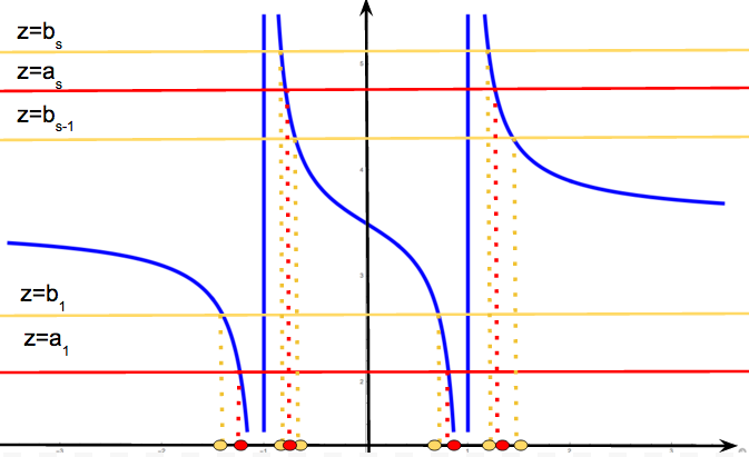
The function $t(z,x,\kappa)$ is decreasing on the intervals $(-\infty,-1),$ $(-1,1)$ and $(1,\infty).$ It follows from the computation of its derivative which is equal to $-\frac{2\kappa(1+z^{2})}{(z^{2}-1)^{2}}$ (recall $\kappa\in(0,1)).$

Thus, since $a_{i}$ and $b_{i}$ interlace the solutions of equations $t(z,x,\kappa)=a_{i}$ and $t(z,x,\kappa)=b_{i}$ will also interlace on each interval of monotonicity. Looking at a general graph of $t(z,x,\kappa)$ and examining the cases we will conclude that the interlacing condition is preserved on the whole line, see Figure 14. Indeed, let us consider the interval $(-\infty,-1).$ Let the lines $y=a_{i}$ and $y=b_{i}$ intersect the graph of $t(z,x,\kappa)$ on this interval. Then the right-most point will be the intersection with the line $y=a_{1}.$ Consider the interval $(-1,1).$ Then the left-most point of intersection will be the intersection with the line $y=b_{s}$ and the right-most point of intersection will be the intersection with the line $y=a_{1}.$ Finally, consider the interval $(1,\infty).$ Let the lines $y=a_{i}$ and $y=b_{i}$ intersect the graph of $t(z,x,\kappa)$ on this interval then the left-most point of intersection will be the intersection with the line $y=b_{s}.$

The leading coefficient of $G_{a}(z,x)$ is $\prod\limits_{i=1}^{2s}(x(1-\kappa)-a_{i})$ and the leading coefficient of $G_{b}(z,x)$ is $\prod\limits_{i=1}^{2s}(x(1-\kappa)-b_{i}).$ First, assume that $x(1-\kappa)-b_{i}\neq 0$ for $i=1,\dots,2s.$ Since $\{\alpha_{i}\}$ and $\{\beta_{i}\}$ interlace the function $G(z,x)$ is always piecewise monotone in $z$ . Examining the cases in Figure 14 we conclude that

\text{ if }\alpha_{1}<\beta_{1},\text{ then }\frac{\prod\limits_{i=1}^{2s}(x(1-\kappa)-a_{i})}{\prod\limits_{i=1}^{2s}(x(1-\kappa)-b_{i})}<0,\text{ and }

\text{ if }\alpha_{1}>\beta_{1},\text{ then }\frac{\prod\limits_{i=1}^{2s}(x(1-\kappa)-a_{i})}{\prod\limits_{i=1}^{2s}(x(1-\kappa)-b_{i})}>0.

Thus, $G(z,x)$ is increasing on every interval $(\beta_{i},\beta_{i+1})$ from $-\infty$ to $\infty.$ There are $2s-1$ such intervals and on every interval there is at least one real solution to $($ 4.6 $),$ see Figure 15. Since the degree of the corresponding polynomial equation is $2s+1$ there exists at most one pair of complex conjugate roots.

∎

Consider the case when $x(1-\kappa)-b_{i}=0$ for some $i.$ Examining the Figure 14 we see that $\alpha_{1}<\beta_{1}<\dots<\beta_{2s-1}<\alpha_{s}.$ Note that

\frac{\prod\limits_{j=1}^{2s}(b_{i}-a_{j})}{2\kappa\prod\limits_{j=1,j\neq i}^{2s}(b_{i}-b_{j})}<0.

Similarly it can be shown that $G(z,x)$ is piecewise increasing. We again can find $2s-2$ roots on every interval $(\beta_{i},\beta_{i+1}).$ Since the degree of the corresponding polynomial equation is $2s$ there exists at most one pair of complex conjugate roots. ∎

Let $x_{0}$ be such that $($ 4.6 $)$ has a pair of complex roots. From the proof of Lemma 4.4 we see that $($ 4.6 $)$ has $2s-1$ distinct real roots when $x(1-\kappa)-b_{i}\neq 0$ for $i=1,\dots,2s$ and $2s-2$ distinct real roots when $x(1-\kappa)-b_{i}=0$ for some $i.$ Due to the Implicit Function Theorem those roots are well-defined in some complex neighborhood $\mathcal{U}$ of $x$ . Let us denote them $z_{j}(x)$ (where $j=1,\dots,2s-1$ or $j=1,\dots,2s-2$ corresponding to two cases mentioned above.)

Lemma 4.5.

The derivative of $z_{j}(x)$ with respect to $x$ at $x_{0}$ is non-negative, for $i=1,\dots 2s-1.$ Moreover, it is equal to zero if and only if $z_{j}(x_{0})=1.$

Proof.

Since $z_{i}(x)$ is given as an implicit function, its derivative can be computed in the following way

(4.8)

z_{i}^{\prime}(x)=-\frac{G^{\prime}_{x}(z,x)}{G^{\prime}_{z}(z,x)-1}.

First, we show that $G^{\prime}_{x}(z,x)\leq 0.$ Recall that

G(z,x)=\frac{(x(1-\kappa)+\frac{2\kappa z}{z^{2}-1}-a_{1})\cdots(x(1-\kappa)+\frac{2\kappa z}{z^{2}-1}-a_{s})}{(x(1-\kappa)+\frac{2\kappa z}{z^{2}-1}-b_{1})\cdots(x(1-\kappa)+\frac{2\kappa z}{z^{2}-1}-b_{s})}.

Thus, when $z\neq\pm 1,$ the statement of the lemma is equivalent to the statement that function

f(y)=\frac{(y-u_{1})\cdots(y-u_{s})}{(y-v_{1})\cdots(y-v_{s})}

is a piecewise decreasing function, where $u_{1}<v_{1}<u_{2}<\dots<u_{n}<v_{n}.$ Thus, it follows that $G^{\prime}_{x}(z,x)<0$ for $z\neq\pm 1.$ Note that $z=-1$ can never be a solution to $($ 4.1 $)$ and when $z=1$ we have $G^{\prime}_{x}(z,x)=0.$

Next, we show that $G^{\prime}_{z}(z_{i}(x_{0}),x_{0})>1.$ From the proof of Lemma 4.4 we know that $G(z,x_{0})$ is an increasing function from $-\infty$ to $\infty$ on every interval $(\beta_{i},\beta_{i+1}).$ Since $x_{0}$ is such that $($ 4.6 $)$ has a pair of complex roots we conclude that there is exactly one real solution $z_{j}(x_{0})$ to $($ 4.6 $)$ on every interval $(\beta_{i},\beta_{i+1}).$ Therefore, $G^{\prime}_{z}(z_{j}(x_{0}),x_{0})>1$ since $G(z,x)-z$ goes from $-\infty$ to $\infty$ on $(\beta_{i},\beta_{i+1})$ and has exactly one root.

Now let us consider $\tilde{x}=x_{0}+i\varepsilon\in\mathcal{U},$ for some very small $\varepsilon.$ From the sign of derivative we obtain $\textup{Im}(z_{i}(\tilde{x}))>0.$ On the other hand,

{\mathbb{Z}}^{\kappa}(\tilde{x})=\exp\left(\int\limits_{\mathbb{R}}\frac{((x_{0}-s)-i\varepsilon)m[ds]}{(x_{0}-s)^{2}+\varepsilon^{2}}\right).

It follows that $\textup{Im}({\mathbb{Z}}^{\kappa}(\tilde{x}))<0.$ Thus, ${\mathbb{Z}}^{\kappa}(x)$ cannot be equal to a real root if the complex roots exist. Therefore, ${\mathbb{Z}}^{\kappa}(x)$ coincides with the unique complex root with negative imaginary part at $x_{0}.$

Finally, from Lemma 4.2 we conclude that

{\mathbb{d}}{\boldsymbol{\eta}}^{\kappa}(x)=-\lim\limits_{\varepsilon\rightarrow 0^{+}}\frac{1}{\pi}\textup{Im}(\textup{St}_{{\boldsymbol{\eta}}^{\kappa}}(x+i\varepsilon))=-\lim\limits_{\varepsilon\rightarrow 0^{+}}\frac{1}{\pi}\textup{Im}\left(\log\left({\mathbb{Z}}^{\kappa}(x+i\varepsilon)\right)\right)=\frac{1}{\pi}\textup{Arg}({\mathbb{z}}^{\kappa}_{+}(x)).

for this class of measures.

Now let us consider a general case of a measure ${\boldsymbol{\eta}}_{\omega}.$ There exists a sequence of measures $\{\eta_{i}\}$ that converges weakly to ${\boldsymbol{\eta}}_{\omega},$ where $\eta_{i}$ is a uniform measure with density one on a sequence of intervals. Then we can pass to the limit in equation (4.4). ∎

Remark 4.6.

Note that the scaling which we use computing ${\boldsymbol{\eta}}^{\kappa}$ is $\frac{1}{(1-\kappa)N},$ while the coordinates of the domain scale as $\frac{1}{N}.$

Definition 4.7.

Let $\mathcal{L}$ be the set of $(\chi,\kappa)$ inside $\mathcal{R}$ such that the density ${\mathbb{d}}{\boldsymbol{\eta}}^{\kappa}(\frac{\chi}{1-\kappa})$ is not equal to $0$ or $1$ . Then $\mathcal{L}$ is called the liquid region. Its boundary $\partial\mathcal{L}$ is called the frozen boundary.

Note that the density ${\mathbb{d}}{\boldsymbol{\eta}}^{\kappa}(\frac{\chi}{1-\kappa})$ is not equal to 0 or 1 if and only if the system (4.1) has a complex solution for $(\chi,\kappa)\in\mathcal{R}.$

5. Frozen boundary

In this section we consider a special case of a rectangular Aztec diamond $\mathcal{R}(N,\Omega,m)$ with

\text{ }\Omega=(A_{1},\dots,B_{1},A_{2},\dots,B_{2},\dots,A_{s},\dots,B_{s}),\text{ where }\sum_{i=1}^{s}(B_{i}-A_{i}+1)=N,\text{ see Figure \ref{fig:boundary}.}

Denote the string $(A_{1},A_{2}\dots,A_{s})$ by $A^{(s)}$ and the string $(B_{1},B_{2}\dots,B_{s})$ by $B^{(s)}.$ We call such domain a rectangular Aztec diamond of type $(N,A^{(s)},B^{(s)})$ .

We are interested in the following asymptotic regime of its growth :

\lim_{N\rightarrow\infty}\frac{A_{i}(N)}{N}=a_{i},\text{ }\lim_{N\rightarrow\infty}\frac{B_{i}(N)}{N}=b_{i},

where $a_{1}<b_{1}<\dots<a_{s}<b_{s}$ are new parameters such that $\sum\limits_{i=1}^{s}(b_{i}-a_{i})=1.$ We will call $s$ the number of segments.

The sequence of signatures $\{\omega(N)\}$ is regular and the limit measure ${\boldsymbol{\eta}}_{\omega}$ is a uniform measure on the union of intervals $[a_{i},b_{i}]$ considered in the proof of the Lemma 4.4.

Theorem 5.1.

The frozen boundary of the limit of a rectangular Aztec diamond of type $(N,A^{(s)},B^{(s)})$ is a rational algebraic curve $C$ with an explicit parametrization (5.3). Moreover, its dual $C^{\vee}$ is of degree $2s$ and is given in the following parametric form

(5.1)

C^{\vee}=\left(\theta,\text{ }\frac{2\theta\Pi_{s}(\theta)}{(\Pi_{s}(\theta)-1)(\Pi_{s}(\theta)+1)}\right),

where

\Pi_{s}(\theta)=\frac{(1-a_{1}\theta)(1-a_{2}\theta)\cdots(1-a_{s}\theta)}{(1-b_{1}\theta)(1-b_{2}\theta)\cdots(1-b_{s}\theta)}.

Remark 5.2.

In projective geometry a dual curve of a given plane curve $C$ is a curve in the dual projective plane consisting of the set of lines tangent to $C$ .

If $C$ is given in a parametric form $C=(x,y)$ then the parametrization of its dual

$C^{\vee}=(x^{\vee},y^{\vee})$ can be found by the following formula:

(5.2)

\begin{cases}x^{\vee}=\frac{y^{\prime}}{yx^{\prime}-xy^{\prime}};\\ y^{\vee}=-\frac{x^{\prime}}{yx^{\prime}-xy^{\prime}}.\end{cases}

We are interested in the dual curve because its parametrization can be written in a simple form and it also encodes the information about the tangents.

Proof.

In the case of a rectangular Aztec diamond of type $(N,A^{(s)},B^{(s)})$ we can rewrite the system of equations (4.1) in the following form:

\begin{cases}\frac{(t-a_{1})(t-a_{2})\cdots(t-a_{s})}{(t-b_{1})(t-b_{2})\cdots(t-b_{s})}=z,\\ F_{\kappa}(z)=\frac{z}{(1-\kappa)}\left(\frac{t}{z}-\frac{1}{z-1}+\frac{\kappa}{1+z}\right)+\frac{z}{z-1}=\frac{\chi}{(1-\kappa)},\end{cases}

Let us express $z$ from the second equation and plug it into the first one. We find that

z^{\pm}(t,\kappa)=\frac{\kappa\pm\sqrt{\kappa^{2}+(t-\chi)^{2}}}{t-\chi}.

From Theorem 4.3 it follows that $(\chi,\kappa)$ belongs to the frozen boundary if and only if the resulting equation has a double root.

Let us introduce the following notation $\textup{L}\Pi_{s}(t):=\log\Pi_{s}(t).$ The condition that the resulting equation has a double root can be rewritten as the following system

\begin{cases}\Pi_{s}(t)=z^{\pm}(t,\kappa),\\ \textup{L}\Pi_{s}(t)^{\prime}=(\log(z^{\pm}(t,\kappa))))^{\prime}.\end{cases}

This system can be solved for $\chi$ and $\kappa$ and we find that

(5.3)

\chi(t)=\frac{\Pi_{s}(t)^{2}\textup{L}\Pi_{s}(t)t+\textup{L}\Pi_{s}(t)t+\Pi_{s}(t)^{2}-1}{(\Pi_{s}(t)^{2}+1)\textup{L}\Pi_{s}(t)}\text{ and }\kappa(t)=-\frac{(\Pi_{s}(\theta)^{2}-1)^{2}}{2(\Pi_{s}(t)^{2}+1)\Pi_{s}(t)\textup{L}\Pi_{s}(t)}.

This gives us the parametric representation of the frozen boundary. In order to compute its dual we use the formula (5.2).

Note that $\Pi_{s}(t)^{\prime}=\Pi_{s}\cdot\textup{L}\Pi_{s}(t).$ Using this relation we get the parametric representation (5.1) of the dual curve after some lengthy computation, where we introduced the parameter $\theta=\frac{1}{t}.$

From the parametric representation it is easy to see that the degree of the dual curve is equal to $2s.$

∎

Definition 5.3.

[33] A degree $d$ real algebraic curve $C\subset\mathbb{R}\textup{P}^{2}$ is winding if

•

It intersects every line $L\subset\mathbb{R}\textup{P}^{2}$ in at least $d-2$ points counting multiplicity;
•

There exists a point $p_{0}\in\mathbb{R}\textup{P}^{2}\setminus C$ called center, such that every line through $p_{0}$ intersects $C$ in $d$ points.

The dual to a winding curve is called a cloud curve.

Proposition 5.4.

The frozen boundary $C$ is a cloud curve of rank $2s,$ where $s$ is the number of segments. Moreover, it is tangent to the following $2s+2$ lines

\mathcal{L}=\{\chi=a_{i}|i=1,\dots,s\}\cup\{\chi=b_{i}|i=1,\dots,s\}\cup\{\kappa=0\}\cup\{\kappa=1\}.

Proof.

We need to check that the dual curve $C^{\vee}=(x,y)$ is winding. Let us write down the equation for the dual curve in terms of the coordinates $x$ and $y.$ Let us denote

P_{a}(x)=(1-a_{1}x)(1-a_{2}x)\dots(1-a_{s}x)\text{ and }P_{b}(x)=(1-b_{1}x)(1-b_{2}x)\dots(1-b_{s}x).

In terms of $x$ and $y$ we get the following equation of $C^{\vee}$

(5.4)

y(P_{a}(x)-P_{b}(x))(P_{a}(x)+P_{b}(x))-2xP_{a}(x)P_{b}(x)=0

Note that $P_{a}(0)=P_{b}(0)=1$ . Thus, the rank of $C$ is $2s.$

We need to compute the intersection of $C^{\vee}$ with any given line in $\mathbb{R}\textup{P}^{2}.$ Let us start with the lines given by $y=cx+d,$ where $c,d\in\mathbb{R}.$ Then the points of intersection satisfy the following equation

(5.5)

(cx+d)(P_{a}(x)-P_{b}(x))(P_{a}(x)+P_{b}(x))=2xP_{a}(x)P_{b}(x).

We will use the same strategy as in Lemma 4.4. We can assume that $a_{1}>0$ since we can move the limit rectangle to the right along the $\chi$ axis, which does not affect the geometric properties of the frozen boundary. The roots of the RHS of equation (5.5) are $\{0,\frac{1}{a_{1}},\frac{1}{b_{1}},\dots,\frac{1}{a_{s}},\dots,\frac{1}{b_{s}}\}.$ Since $\{a_{i}\}$ and $\{b_{i}\}$ interlace, all the roots of $p_{-}=P_{a}(x)-P_{b}(x)$ and $p_{+}=P_{a}(x)+P_{b}(x)$ are real and there are $2s-1$ distinct roots. Moreover, there exist two roots of $p_{\pm}$ in every interval $(\frac{1}{a_{i+1}},\frac{1}{a_{i}})$ and the point $\frac{1}{b_{i}}$ lies in between those roots. Therefore, the roots of the polynomial given by the LHS of (5.5) interlace with the roots of the polynomial given by the RHS with probably an exception of an interval containing the zero of $cx+d.$ So we have found at least $2s-2$ real points of intersection of our curve with lines of the form $y=cx+d.$

Next, consider the lines $x=d.$ The intersection will be at infinity. We need to consider the homogenized polynomial that defines our curve adding the third homogeneous coordinate $z$ .

y(P_{a}(x,z)-P_{b}(x,z))(P_{a}(x,z)+P_{b}(x,z))-2xP_{a}(x,z)P_{b}(x,z)=0,

P_{a}(x,z)=(z-a_{1}x)(z-a_{2}x)\dots(z-a_{s}x)\text{ and }P_{b}(x,z)=(z-b_{1}x)(z-b_{2}x)\dots(z-b_{s}x).

The homogeneous form of the equation of the line is $x=dz.$ Thus, we see that this line intersects the curve at the point $(0:1:0)$ with multiplicity $2s-1.$ The case of the line $z=0$ is analogous.

Note that due to the computation above if we choose a point $p_{0}$ on the line $y=0$ outside the interval $(0,\frac{1}{a_{1}})$ any line passing through $p_{0}$ will intersect the curve $C^{\vee}$ at at least $2s-1$ real points. Therefore, any line through $p_{0}$ will intersect $C^{\vee}$ at exactly $2s$ real points. So the point $p_{0}$ can be chosen to be the center.

Notice that the points $(x,y)=(0,\frac{1}{a_{i}})$ as well as $(x,y)=(0,\frac{1}{b_{i}})$ belong to $C^{\vee}.$ The roots of $(P_{a}(x)-P_{b}(x))(P_{a}(x)+P_{b}(x))$ correspond to $2s-1$ points of tangency of $C$ with the line $\kappa=0.$ Also, when $x=0$ the $y$ coordinate of $C^{\vee}$ is $1$ , which corresponds to the tangent $\kappa=1$ of $C.$ From these the second statement of the proposition follows.

∎

Remark 5.5.

From (5.1) and (5.3) we see that the points of tangency of $C=(\chi(\theta),\kappa(\theta))$ with $\kappa=0,$ that is, with the side of rectangle with nontrivial boundary conditions, are precisely the roots of

\prod\limits_{i=1}^{s}\frac{x-a_{i}}{x-b_{i}}=\pm 1.

6. Central Limit Theorem

In this section we study the fluctuations of the limit shape. In particular, we show that the fluctuations are described by the Gaussian Free Field. There are two major steps in the proof of this result. First, we describe the complex structure on the liquid region that leads to the appearance of the Gaussian Free Field as the limit object. Next, we give an overview of the results from [10] that allow us to perform the computations to establish the main result Theorem 6.3.

6.1. Characterization of the liquid region

By Theorem 4.3 $(\chi,\kappa)\in\mathcal{L}$ (see definition 4.7 and the remark above it) if and only if the system of equations (4.1) has complex roots. Let us recall it

\begin{cases}\mathbf{F}_{\kappa}(z{,}t)=\frac{\chi}{(1-\kappa)},\\ \textup{St}_{{\boldsymbol{\eta}}_{\omega}}(t)=\log(z),\end{cases}

where

\mathbf{F}_{\kappa}(z,t)=\frac{z}{(1-\kappa)}\Big(\frac{t}{z}-\frac{1}{(z-1)}+\frac{\kappa}{1+z}\Big)+\frac{z}{z-1}.

From the first equation we find that

(6.1)

z_{\pm}(\chi,\kappa)(t)=\frac{\kappa\pm\sqrt{\kappa^{2}+(t-\chi)^{2}}}{t-\chi}\text{ and }t=\frac{\chi z^{2}+2\kappa z-\chi}{z^{2}-1}.

It follows that $z_{\pm}(\chi,\kappa)$ is complex if and only if $t$ is (if one of them is real then the other one has to be real too).

Let $\mathbb{H}$ be the upper half-plane of the complex plane.

Lemma 6.1.

Let $t\in\mathbb{H}.$ Then there exists $z(t)$ such that $(z(t),t)$ is the solution to $($ 4.1 $)$ if and only if the following equation holds

(6.2)

p^{\chi,\kappa}(t)\colon=\chi-\left(t+\kappa\left(\frac{1}{\exp(-\textup{St}_{{\boldsymbol{\eta}}_{\omega}}(t))-1}+\frac{1}{\exp(-\textup{St}_{{\boldsymbol{\eta}}_{\omega}}(t))+1}\right)\right)=0.

Proof.

Let $t$ be a solution to (6.2). Let us express $\textup{St}_{{\boldsymbol{\eta}}_{\omega}}(t))$ from this equation. We find that

\textup{St}_{{\boldsymbol{\eta}}_{\omega}}(t)=\log(z_{\pm}(\chi,\kappa)(t)).

Picking the right sign we find $z(t)$ which solves (4.1). A direct computations shows that if $(z,t)$ is a solution of 4.1 then $t$ is a solution to (6.2).

∎

Note that from Lemma 4.4 using Rouché’s theorem it follows that there exists a unique solution $t\in\mathbb{H}$ of (6.2). Denote

S(t):=\textup{St}_{{\boldsymbol{\eta}}_{\omega}}(t)

for convenience.

The next Proposition defines a homeomorphism between the liquid region and the upper half-plane $\mathbb{H}.$

Proposition 6.2.

Let

T_{\mathcal{L}}\colon\mathcal{L}\rightarrow\mathbb{H}

map $(\chi,\kappa)\in\mathcal{L}$ to the corresponding unique root of (6.2) in $\mathbb{H}.$ Then, $T_{\mathcal{L}}$ is a homeomorphism with inverse $t\rightarrow(\chi_{\mathcal{L}}(t),\kappa_{\mathcal{L}}(t))$ for all $t\in\mathbb{H}$ , given by

(6.3)

\chi_{\mathcal{L}}(t)=t+\frac{\exp(S(\bar{t}))(\exp(2S(t))-1)(t-\bar{t})}{(\exp(S(t))-\exp(S(\bar{t})))(1+\exp(S(t)+S(\bar{t})))};

(6.4)

\kappa_{\mathcal{L}}(t)=-\frac{(\exp(2S(t))-1)(\exp(2S(\bar{t}))-1)(t-\bar{t})}{2(\exp(S(t))-\exp(S(\bar{t})))(1+\exp(S(t)+S(\bar{t})))}.

Proof.

The proof is completely analogous to the proof of Theorem 2.1 in [18]. For the reader’s convenience we will present it.

We need to show

(1)

$\mathcal{L}$ is non-empty. More precisely, we will show that whenever $|t|$ is large enough $t\rightarrow(\chi_{\mathcal{L}}(t),\kappa_{\mathcal{L}}(t))\in\mathcal{R}$ and (6.2) holds. Then it follows that $(\chi_{\mathcal{L}}(t),\kappa_{\mathcal{L}}(t))\in\mathcal{L}$ for such $t.$
(2)

$\mathcal{L}$ is open.
(3)

$T_{\mathcal{L}}\colon\mathcal{L}\rightarrow\mathbb{H}$ is continuous.
(4)

$T_{\mathcal{L}}\colon\mathcal{L}\rightarrow\mathbb{H}$ is injective.
(5)

$T_{\mathcal{L}}\colon\mathcal{L}\rightarrow T_{\mathcal{L}}(\mathcal{L})$ has inverse for all $t\in T_{\mathcal{L}}(\mathcal{L}).$
(6)

$T_{\mathcal{L}}(\mathcal{L})=\mathbb{H}.$

Let us start with (1). Fix $t\in\mathbb{H}$ and define

(6.5)

(\chi,\kappa)=(\chi_{\mathcal{L}}(t),\kappa_{\mathcal{L}}(t))

using (6.3) and (6.4) . Then the following equation holds

(6.6)

(\exp(2S(t))-1)(t-\chi)=2\exp(S(t))\kappa.

It is equivalent to (6.2).

Second, let us look at the Taylor expansions for $\chi_{\mathcal{L}}(t)$ and $\kappa_{\mathcal{L}}(t),$ when $|t|$ goes to infinity.

Let $a,b\in\mathbb{R}$ be such that $\textup{Support}({\boldsymbol{\eta}}_{\omega})\subset[a,b].$ We have the following asymptotics for the Stieltjes transform

S(t)=\frac{1}{t}+\frac{\alpha}{t^{2}}+\frac{\beta}{t^{3}}+O(|t|^{-4}),

where $\alpha=\int_{a}^{b}x\text{ }{\boldsymbol{\eta}}_{\omega}[dx]$ and $\beta=\int_{a}^{b}x^{2}{\boldsymbol{\eta}}_{\omega}[dx].$ After some computation we get

\chi=\alpha+O(|t|^{-1})\text{ and }\kappa=1+\left(\alpha^{2}-\beta-\frac{1}{6}\right)\frac{1}{|t|^{2}}+O(|t|^{-3}).

Recall that by our assumptions ${\boldsymbol{\eta}}_{\omega}$ is a probability measure such that $b-a>1$ since ${\boldsymbol{\eta}}_{\omega}\leq\lambda,$ where $\lambda$ is the Lebesgue measure. Therefore, we have

a+\frac{1}{2}=\int_{a}^{a+1}xdx<\alpha<\int_{b-1}^{b}xdx=b-\frac{1}{2}.

Similarly,

\beta-\alpha^{2}>\frac{1}{2}\int\int_{0}^{1}(x-y)^{2}dxdy=\frac{1}{12}.

It follows that $(\chi,\kappa)\in(a+\frac{1}{2},b-\frac{1}{2})\times(0,1)$ whenever $|t|$ is chosen to be sufficiently large. This proves (1).

Consider (2). Let $(\chi_{1},\kappa_{1})\in\mathcal{L}$ and $t_{1}=T_{\mathcal{L}}(\chi_{1},\kappa_{1}).$ We will show that $(\chi_{2},\kappa_{2})\in\mathcal{L}$ whenever $|\chi_{1}-\chi_{2}|$ and $|\kappa_{1}-\kappa_{2}|$ are sufficiently small. Fix $\epsilon>0$ such that $B(t_{1},\epsilon)\subset\mathbb{H}$ . Let $t_{1}$ is the unique root of $p^{\chi_{1},\kappa_{1}}(t)$ in $\mathbb{H},$ the extreme value theorem gives,

\inf\limits_{t\in\partial B(t_{1},\epsilon)}|p^{\chi_{1},\kappa_{1}}(t)|>0.

Also,

(6.7)

|p^{\chi_{1},\kappa_{1}}(t)-p^{\chi_{2},\kappa_{2}}(t)|<\epsilon

for any $\epsilon>0,$ whenever $|\chi_{1}-\chi_{2}|$ and $|\kappa_{1}-\kappa_{2}|$ are sufficiently small.

Whenever $|\chi_{1}-\chi_{2}|$ and $|\kappa_{1}-\kappa_{2}|$ are sufficiently small $|p^{\chi_{1},\kappa_{1}}(t)|>|p^{\chi_{1},\kappa_{1}}_{+}(t)-p^{\chi_{2},\kappa_{2}}_{+}(t)|.$ Rouchés Theorem implies that $p^{\chi_{1},\kappa_{1}}_{+}(t)$ has a root in $B(t,\epsilon).$

Consider (3). The analysis is very similar to part (2) and is tautologically the same as in [18].

Consider (4). Suppose there exist $(\chi_{1},\kappa_{1}),(\chi_{2},\kappa_{2})\in\mathcal{L}$ such that $T_{\mathcal{L}}(\chi_{1},\kappa_{1})=T_{\mathcal{L}}(\chi_{2},\kappa_{2})=t\in\mathbb{H}.$

From (6.2) we get

t=\frac{\kappa_{1}\chi_{1}-\kappa_{2}\chi_{2}}{\kappa_{1}-\kappa_{2}}.

But then $t\in\mathbb{R}$ whenever $\kappa_{1}\neq\kappa_{2},$ which contradicts $t\in\mathbb{H}.$ Thus, $\kappa_{1}=\kappa_{2}\in(0,1).$ It follows $\chi_{1}=\chi_{2}$ too.

Consider (5). This follows from (6.6).

Consider (6). We already know that $T_{\mathcal{L}}(\mathcal{L})$ is open and homeomorphic to $\mathcal{L}$ . Suppose there exists $t\in\partial T_{\mathcal{L}}(\mathcal{L})$ such that $t\in\mathbb{H}\setminus T_{\mathcal{L}}(\mathcal{L}).$ Let $\{t_{n}\}\in T_{\mathcal{L}}(\mathcal{L})$ be a sequence that converges to $t$ as $n\rightarrow\infty$ . There exists a subsequence of $\{(\chi_{\mathcal{L}}(t_{n}),\kappa_{\mathcal{L}}(t_{n}))\}$ that converges to some $(\chi,\kappa).$ Then we can pass to the limit in (6.2) and we see that $(\chi,\kappa)\in\mathcal{R}$ and $t=T_{\mathcal{L}}(\chi,\kappa).$ This is a contradiction. ∎

6.2. Gaussian Free Field

A Gaussian family is a collection of jointly Gaussian random variables $\{\xi_{a}\}_{a\in\Upsilon}$ indexed by an arbitrary set $\Upsilon$ . We assume that all our random variables are centered, that is

\mathbf{E}\xi_{u}=0,\qquad\mbox{ for all }u\in\Upsilon.

Any Gaussian family gives rise to a covariance kernel $\mathrm{Cov}:\Upsilon\times\Upsilon\to\mathbb{R}$ defined by

\mathrm{Cov}(u_{1},u_{2})=\mathbf{E}(\xi_{u_{1}}\xi_{u_{2}}).

Assume that a function $\tilde{C}:\Upsilon\times\Upsilon\to\mathbb{R}$ is such that for any $n\geq 1$ and $u_{1},\dots,u_{n}\in\Upsilon$ , $[\tilde{C}(u_{i},u_{j})]_{i,j=1}^{n}$ is a symmetric and positive-definite matrix. Then there exists a centered Gaussian family with the covariance kernel $\tilde{C}$ (see e.g. [11]).

Let $C_{0}^{\infty}$ be the space of smooth real–valued compactly supported test functions on the upper half-plane $\mathbb{H}$ . Let us set

\tilde{G}(z,w):=-\frac{1}{2\pi}\ln\left|\frac{z-w}{z-\bar{w}}\right|,\qquad z,w\in\mathbb{H}.

This is the Green function of the Laplace operator on $\mathbb{H}$ with Dirichlet boundary conditions. Define a function $C:C_{0}^{\infty}\times C_{0}^{\infty}\to\mathbb{R}$ via

C(f_{1},f_{2}):=\int_{\mathbb{H}}\int_{\mathbb{H}}f_{1}(z)f_{2}(w)\tilde{G}(z,w)dzd\bar{z}dwd\bar{w}.

The Gaussian Free Field (GFF) $\mathfrak{G}$ on $\mathbb{H}$ with zero boundary conditions can be defined as a Gaussian family $\{\xi_{f}\}_{f\in C_{0}^{\infty}}$ with covariance kernel $C$ .

The integrals $\int f(z)\mathfrak{G}(z)dz$ over finite contours in $\mathbb{H}$ with continuous functions $f(z)$ make sense, cf. [41], while the field $\mathfrak{G}$ cannot be defined as a random function on $\mathbb{H}$ .

6.3. Statement of the theorem

Consider a rectangular Aztec diamond $\mathcal{R}(N,\Omega,m).$ Let $\omega$ be a signature corresponding to the boundary row under Construction 2.7.

We have defined a probability measure $P^{N}_{\omega}$ on the sets of signatures

\mathcal{S}^{N}=(\mu^{(N)},\nu^{(N)},\dots,\mu^{(1)},\nu^{(1)}),

see equation (2.8).

Let us define a function $\Delta^{N}$ on $\mathbb{R}_{\geq 0}\times\mathbb{R}_{\geq 0}\times\mathcal{S}\to\mathbb{N}$ via

(6.8)

\Delta^{N}\colon(x,y,(\mu^{(N)},\nu^{(N)},\dots,\mu^{(1)},\nu^{(1)}))\rightarrow\\ \sqrt{\pi}\left|\left\{1\leq s\leq N-\lfloor y\rfloor:\mu^{(N-\lfloor y\rfloor)}_{s}+(N-\lfloor y\rfloor)-s\geq x\right\}\right|.

Recall the definition (3.16) of $\Delta^{N}_{D}(i,j),$ where $D\in\mathfrak{D}(N,\Omega,m)$ and $(i,j)$ is a lattice vertex in $\mathcal{R}(N,\Omega,m).$ Its domain of definition can be extended to $(i,j)\in\mathbb{R}_{\geq 0}\times\mathbb{R}_{\geq 0}.$ We get

(6.9)

\Delta^{N}(i,j,\mu(D))=\sqrt{\pi}\Delta^{N}_{D}(i,j).

Here $\mu(D)$ is the sequence of signatures corresponding to $Y(D),$ where $Y$ is a bijection between $\mathfrak{D}(N,\Omega,m)$ and $\mathcal{S}(N,\Omega,m),$ see Theorem 2.9.

Let us denote by $\Delta^{N}_{\mathfrak{D}}(x,y)$ the pushforward of the measure $P^{N}_{\omega}$ on $\mathcal{S}^{N}$ with respect to $\Delta^{N}$ . Note that due to Proposition 2.13 $\Delta^{N}_{\mathfrak{D}}(x,y)$ coincides with the pushforward of the uniform measure on $\mathfrak{D}(N,\Omega,m)$ with respect to $\Delta_{D}.$

Let us carry $\Delta^{N}_{\mathfrak{D}}(x,y)$ over to $\mathbb{H}$ in the following way

{\mathbb{\Delta}}_{\mathfrak{D}}^{N}(z):=\Delta_{\mathfrak{D}}^{N}(N\chi_{\mathcal{L}}(z),N\kappa_{\mathcal{L}}(z)),\qquad z\in\mathbb{H},

where $\chi_{\mathcal{L}}(z)$ is defined by (6.3) and $\kappa_{\mathcal{L}}(z)$ is defined by (6.4). For a real number $0<\kappa<1$ and an integer $j$ define a moment of the random function ${\mathbb{\Delta}}_{\mathfrak{D}}^{N}$ as

(6.10)

M^{\kappa}_{j}=\int_{-\infty}^{+\infty}\chi^{j}\left({\mathbb{\Delta}}_{\mathfrak{D}}^{N}(N\chi,N\kappa)-\mathbf{E}{\mathbb{\Delta}}_{\mathfrak{D}}^{N}(N\chi,N\kappa)\right)d\chi.

Also define the corresponding moment of GFF via

\mathcal{M}^{\kappa}_{j}=\int_{z\in\mathbb{H};\kappa_{\mathcal{L}}(z)=\kappa}\chi_{\mathcal{L}}(z)^{j}\mathfrak{G}(z)\frac{d\chi_{\mathcal{L}}(z)}{dz}dz.

Theorem 6.3 (Central Limit Theorem).

Let ${\mathbb{\Delta}}_{\mathfrak{D}}^{N}(z)$ be a random function corresponding to the uniformly random domino tiling of the rectangular Aztec diamond in the way described above. Then

{\mathbb{\Delta}}_{\mathfrak{D}}^{N}(z)-\mathbf{E}{\mathbb{\Delta}}_{\mathfrak{D}}^{N}(z)\xrightarrow[N\to\infty]{}\mathfrak{G}(z).

In more details, as $N\to\infty$ , the collection of random variables $\{M^{\kappa}_{j}\}_{1\geq\kappa>0;j\in\mathbb{N}}$ converges, in the sense of finite-dimensional distributions, to $\{\mathcal{M}^{\kappa}_{j}\}_{1\geq\kappa>0;j\in\mathbb{N}}$ .

Remark 6.4.

Due to Lemma 3.11 the corresponding statement for the random height function $h_{\mathfrak{D}}$ follows.

Remark 6.5.

Theorem 6.3 establishes the convergence for a certain limited class of test functions. It is very plausible that the statement can be extended to a larger class of test functions, but we do not address this question here.

6.4. Schur generating functions

For the proof of Theorem 6.3 we will use the moment method of Schur-generating functions from [10]. In this section we will recall necessary notions and results from [10] (Theorems 6.7 and 6.8 below). After this we will apply them to our measure (Theorem 6.9).

Definition 6.6.

We say that a sequence of probability measures $\rho(N)$ on $\mathbb{GT}_{N}$ is CLT-appropriate if theirs Schur generating functions $S^{U(N)}_{\rho(N)}(x_{1},\dots,x_{N})$ satisfy the following condition: For any fixed $k\in\mathbb{N}$ we have

•

\lim_{N\to\infty}\frac{\partial_{i}\ln S^{U(N)}_{\rho(N)}(x_{1},x_{2},\dots,x_{k},1^{N-k})}{N}=F(x_{i}),\qquad 1\leq i\leq k,

•

\lim_{N\to\infty}\partial_{i}\partial_{j}\ln S^{U(N)}_{\rho(N)}(x_{1},x_{2},\dots,x_{k},1^{N-k})=G(x_{i},x_{j}),\qquad 1\leq i,j\leq k,\ i\neq j,

where the functions $F(x)$ and $G(x,y)$ are holomorphic in a neighborhood of the unity, and the convergence is uniform over an open complex neighborhood of $(x_{1},\dots,x_{k})=(1^{k})$ . Note that the functions in the left-hand side of these equations depend on $k$ variables, while the the functions in the right-hand side depend on 1 or 2 variables, respectively.

For $\lambda\in\mathbb{GT}_{k_{1}},\mu\in\mathbb{GT}_{k_{2}}$ , $k_{1}\geq k_{2}$ , let us introduce the coefficients $\mathrm{pr}_{k_{1}\to k_{2}}(\lambda\to\mu)$ (the construction is similar to the one from Section 2) via

\frac{s_{\lambda}(x_{1},\dots,x_{k_{2}},1^{k_{1}-k_{2}})}{s_{\lambda}(1^{k_{1}})}=\sum_{\mu\in\mathbb{GT}_{k_{2}}}\mathrm{pr}_{k_{1}\to k_{2}}(\lambda\to\mu)\frac{s_{\mu}(x_{1},\dots,x_{k_{2}})}{s_{\mu}(1^{k_{2}})}.

For a symmetric function $g(x_{1},\dots,x_{N})$ we define the coefficients $\mathrm{st}_{(g)}^{(N)}(\lambda\to\mu)$ , for $\lambda\in\mathbb{GT}_{N}$ , $\mu\in\mathbb{GT}_{N}$ , via

g(x_{1},\dots,x_{N})\frac{s_{\lambda}(x_{1},\dots,x_{N})}{s_{\lambda}(1^{N})}=\sum_{\mu\in\mathbb{GT}_{N}}\mathrm{st}_{(g)}^{(N)}(\lambda\to\mu)\frac{s_{\mu}(x_{1},\dots,x_{N})}{s_{\mu}(1^{N})},

where we assume that the function $g(x_{1},\dots,x_{N})$ is such that the number of terms in the summation in the right-hand side is finite for all $\lambda$ .

Let $m$ be a positive integer and let $0<a_{1}\leq\dots\leq a_{m}=1$ be reals. Let $\rho_{N}=\rho_{[a_{m}N]}$ be a CLT-appropriate measure on $\mathbb{GT}_{[a_{m}N]}$ with the Schur generating function $S_{N}$ , and let $g_{1}(x_{1},\dots,x_{[a_{1}N]})$ , $\dots$ , $g_{m}(x_{1},\dots,x_{[a_{m}N]})$ be a collection of Schur generating functions of some CLT-appropriate probability measures.

Let us define the probability measure on the set

\mathbb{GT}_{[a_{m}N]}\times\mathbb{GT}_{[a_{m}N]}\times\mathbb{GT}_{[a_{m-1}N]}\times\mathbb{GT}_{[a_{m-1}N]}\times\dots\times\mathbb{GT}_{[a_{1}N]}\times\mathbb{GT}_{[a_{1}N]}.

That is, we need to define the probability of a collection of signatures $(\mu^{(m)}$ , $\nu^{(m)}$ , $\mu^{(m-1)}$ , $\nu^{(m-1)}$ , $\dots$ , $\mu^{(1)}$ , $\nu^{(1)})$ , where $\mu^{(i)}$ , $\nu^{(i)}$ are signatures of length $[a_{i}N]$ , $i=1,2,\dots,m$ . Let us do this in the following way.

Let

	$\displaystyle H_{m}^{\mu}(x_{1},\dots,x_{[a_{m}N]}):=S_{N}(x_{1},\dots,x_{[a_{m}N]}),$
	$\displaystyle H_{m}^{\nu}(x_{1},\dots,x_{[a_{m}N]}):=H_{m}^{\mu}(x_{1},\dots,x_{[a_{m}N]})g_{m}(x_{1},\dots,x_{[a_{m}N]}),$
	$\displaystyle H_{m-1}^{\mu}(x_{1},\dots,x_{[a_{m-1}N]}):=H_{m}^{\nu}(x_{1},\dots,x_{[a_{m-1}N]},1^{[a_{m}N]-[a_{m-1}N]}),$
	$\displaystyle H_{m-1}^{\nu}(x_{1},\dots,x_{[a_{m-1}N]}):=H_{m-1}^{\mu}(x_{1},\dots,x_{[a_{m-1}N]})g_{m-1}(x_{1},\dots,x_{[a_{m-1}N]}),$
	$\displaystyle\dots\dots\dots\dots\dots$
	$\displaystyle H_{1}^{\mu}(x_{1},\dots,x_{[a_{1}N]}):=H_{2}^{\nu}(x_{1},\dots,x_{[a_{2}N]},1^{[a_{2}N]-[a_{1}N]}),$
	$\displaystyle H_{1}^{\nu}(x_{1},\dots,x_{[a_{1}N]}):=H_{1}^{\mu}(x_{1},\dots,x_{[a_{1}N]})g_{1}(x_{1},\dots,x_{[a_{1}N]}),$

Assume that the coefficients $\mathrm{st}^{[a_{t}N]}_{g_{t}}(\mu\to\nu)$ , $t=1,\dots,s$ are positive for all $t$ , $\mu\in\mathbb{GT}_{[a_{t}N]}$ , $\nu\in\mathbb{GT}_{[a_{t}N]}$ (again, we also assume that the linear decomposition which defines these coefficients is finite).

We define the probability of the configuration $(\mu^{(m)},\nu^{(m)},\dots,\mu^{(1)},\nu^{(1)})$ by

(6.11)

\mathcal{P^{N}}(\mu^{(m)},\nu^{(m)},\mu^{(m-1)},\nu^{(m-1)},\dots,\mu^{(1)},\nu^{(1)})\\ :=\rho_{N}(\mu^{(m)})\mathrm{st}^{[a_{1}N]}_{g_{1}}(\mu^{(1)}\to\nu^{(1)})\prod_{i=2}^{m}\mathrm{st}^{[a_{i}N]}_{g_{i}}(\mu^{(i)}\to\nu^{(i)})\mathrm{pr}_{[a_{i}N]\to[a_{i-1}N]}(\nu^{(i)}\to\mu^{(i-1)}).

The conditions above guarantee the existence of the following limits:

\lim_{N\to\infty}\frac{\partial_{i}\ln H^{\mu}_{t}(x_{1},x_{2},\dots,x_{k},1^{N-k})}{N}=:F_{t}(x_{i}),\qquad 1\leq i\leq k

\lim_{N\to\infty}\partial_{i}\partial_{j}\ln H^{\mu}_{t}(x_{1},x_{2},\dots,x_{k},1^{N-k})=:G_{t}(x_{i},x_{j}),\qquad 1\leq i,j\leq k,\ i\neq j,

for any $t=1,2,\dots,m$ .

Let

p_{k;t}:=\sum_{i=1}^{[a_{t}N]}\left(\mu^{(t)}_{i}+[a_{t}N]-i\right)^{k},

be (shifted) moments of these signatures. These functions become random when we consider the random sequence $(\mu^{(m)},\nu^{(m)},\dots,\mu^{(1)},\nu^{(1)})$ distributed according to the probability measure $\mathcal{P}^{N}$ . We are interested in the asymptotic behavior of these functions.

Theorem 6.7.

$($ [10] $)$ In the notations above, the collection of random functions

\{N^{-k}(p_{k;t}-\mathbf{E}p_{k;t})\}_{t=1,\dots,m;k\in\mathbb{N}}

is asymptotically Gaussian with the limit covariance

\lim_{N\to\infty}N^{-k_{1}-k_{2}}\mathrm{cov}\left(p_{k_{1};t_{1}},p_{k_{2};t_{2}}\right)=\frac{a_{1}^{k_{1}}a_{2}^{k_{2}}}{(2\pi{\mathbf{i}})^{2}}\oint_{|z|=\varepsilon}\oint_{|w|=2\varepsilon}\left(\frac{1}{z}+1+(1+z)F_{t_{1}}(1+z)\right)^{k_{1}}\\ \times\left(\frac{1}{w}+1+(1+w)F_{t_{2}}(1+w)\right)^{k_{2}}\left(G_{t_{2}}(z,w)+\frac{1}{(z-w)^{2}}\right)dzdw,

where $\varepsilon\ll 1$ and $1\leq t_{1}\leq t_{2}\leq m$ .

Now we will apply this theorem to our case. Consider $N\rightarrow\infty$ asymptotics of a rectangular Aztec diamond $\mathcal{R}(N,\Omega(N),m(N)).$ We assume that the sequence of signatures $\omega(N)$ corresponding to the first row is regular and the sequence of measures $\{m[\omega(N)]\}$ weakly converge to ${\boldsymbol{\eta}}_{\omega}.$ Our probability measure on the set of domino tilings $\mathfrak{D}(N,\Omega,m)$ defined by (8.3) has $\rho$ concentrated on a single signature (but with a non-trivial asymptotic behavior), and the functions $g_{i}$ are equal to the powers of $\prod_{i}(1+x_{i})$ times a constant.

Let us recall some results from [10]. We will need the following theorem.

Theorem 6.8 ([24], [10]).

Suppose that $\lambda(N)\in\mathbb{GT}_{N}$ , $N=1,2,\dots$ is a regular sequence of signatures such that

\lim_{N\to\infty}m[\lambda(N)]={\boldsymbol{\eta}}.

Then we have

(6.12)

\lim_{N\to\infty}\partial_{1}\partial_{2}\log\left(\frac{s_{\lambda(N)}(x_{1},x_{2},\dots,x_{k},1^{N-k})}{s_{\lambda(N)}(1^{N})}\right)\\ =\partial_{1}\partial_{2}\log\left(1-(x_{1}-1)(x_{2}-1)\frac{x_{1}H^{\prime}_{\boldsymbol{\eta}}(x_{1})-x_{2}H^{\prime}_{{\boldsymbol{\eta}}}(x_{2})}{x_{1}-x_{2}}\right),

where the convergence is uniform over an open complex neighborhood of $(x_{1},\dots,x_{k})=(1^{k})$ .

Construction 2.7 assigns to each row with number $[2\kappa N]$ of $\mathcal{R}(N,\Omega,m)$ a Young diagram given by a $[(1-\kappa)N]$ -tuple $\mu^{([(1-\kappa)N])}_{i}=(\mu_{1},\dots,\mu_{[(1-\kappa)N]}).$ We define the moment function as

p_{j}^{\kappa}:=\sum_{i=1}^{[(1-\kappa)N]}\left(\mu^{([(1-\kappa)N])}_{i}+[(1-\kappa)N]-i\right)^{j}.

Theorem 6.9.

In the notations above, the collection of random functions

\{N^{-k}(p_{j}^{\kappa}-\mathbf{E}p_{j}^{\kappa})\}_{0<\kappa\leq 1;j\in\mathbb{N}}

is asymptotically Gaussian with the limit covariance

(6.13)

\lim_{N\to\infty}N^{-j_{2}-j_{1}}\mathrm{cov}\left(p_{j_{1}}^{\kappa_{1}},p_{j_{2}}^{\kappa_{2}}\right)=\frac{(1-\kappa_{1})^{j_{1}}(1-\kappa_{2})^{j_{2}}}{(2\pi{\mathbf{i}})^{2}}\oint_{|z|=\varepsilon}\oint_{|w|=2\varepsilon}\left(\frac{1}{z}+1+(1+z)F_{1}(1+z)\right)^{j_{1}}\\ \times\left(\frac{1}{w}+1+(1+w)F_{2}(1+w)\right)^{j_{2}}Q(z,w)dzdw,

where $\varepsilon\ll 1$ and $1\geq\kappa_{1}\geq\kappa_{2}>0$ ,

F_{1}(z)=\frac{1}{1-\kappa_{1}}H^{\prime}_{{\boldsymbol{\eta}}_{\omega}}(1+z)+\frac{\kappa_{1}}{(1-\kappa_{1})(z+2)},

F_{2}(w)=\frac{1}{1-\kappa_{2}}H^{\prime}_{{\boldsymbol{\eta}}_{\omega}}(1+w)+\frac{\kappa_{2}}{(1-\kappa_{2})(w+2)}

and

Q(z,w)=\partial_{z}\partial_{w}\left(\log\left(1-zw\frac{(1+z)H^{\prime}_{{\boldsymbol{\eta}}_{\omega}}(1+z)-(1+w)H^{\prime}_{{\boldsymbol{\eta}}_{\omega}}(1+w)}{z-w}\right)\right)+\frac{1}{(z-w)^{2}}.

Proof.

It immediately follows from Theorem 6.7, Theorem 6.8 and Lemma 3.7.

∎

Remark 6.10.

Let us make several comments about this result.

The general mechanism of Theorem 6.7 automatically produces the central limit theorem for moments. However, a further analysis is necessary in order to show that the obtained covariance matches the one coming from the Gaussian Free Field.

One can use another generator of the semigroup with respect to the quantized free convolution $($ see Remark 3.9 $)$ . In the case of rectangular Aztec diamonds we used

\prod\limits_{i}(1+x_{i})/2=\prod\limits_{i}(1+\frac{1}{2}(x_{i}-1)),

which can be understood as an extreme beta character with parameter $\frac{1}{2}$ . Instead, one can use formulas

\prod(1+\beta(x_{i}-1))\text{ or }\prod(1+\alpha(x_{i}-1))^{-1},\text{ where }0<\beta<1,\text{ and }0<\alpha<+\infty.

One can immediately generalize our results to the case when the probability measure comes from these formulas. We give some details for $0<\beta<1$ case in 8. Appendix A.

One can also analyze another types of processes, in particular, Schur processes $($ or ensembles of non-intersecting paths, see Section 2.3 $)$ . In this case one needs to suitably modify Theorem 6.7; these generalizations quite straightforwardly follow from the technique of [10]. After this, one can apply the technique of this paper in order to extract all necessary information about limit shapes, frozen boundary, and global fluctuations.

Finally, let us remark that while the moment method proved to be very convenient for the study of the global behavior of our model, it does not give insight on the local behavior. Nevertheless, it is possible to extract some information about it from the known results on lozenge tilings. We discuss it in 9. Appendix B.

6.5. Proof of Theorem 6.3

The goal of this section is to obtain Theorem 6.3 from Theorem 6.9.

First, let us make a change of variables

\tilde{z}=S_{{\boldsymbol{\eta}}_{\omega}}^{(-1)}\left(\log(1+z)\right),\qquad\tilde{w}=S_{{\boldsymbol{\eta}}_{\omega}}^{(-1)}\left(\log(1+w)\right),

in equation (6.13).

Using the connection between $S_{{\boldsymbol{\eta}}_{\omega}}(z)$ and $H^{\prime}_{{\boldsymbol{\eta}}_{\omega}}(z)$ (see (3.7)), we have

	$\displaystyle\frac{1}{z}+1+\frac{(1+z)H^{\prime}_{{\boldsymbol{\eta}}_{\omega}}(z+1)}{1-\kappa_{1}}=\frac{1}{1-\kappa_{1}}\left(\frac{1}{\tilde{z}}+\frac{\kappa_{1}}{\exp(-S_{{\boldsymbol{\eta}}_{\omega}}(\tilde{z}))-1}\right),$
	$\displaystyle\frac{1}{w}+1+\frac{(1+w)H^{\prime}_{{\boldsymbol{\eta}}_{\omega}}(w+1)}{1-\kappa_{2}}=\frac{1}{1-\kappa_{2}}\left(\frac{1}{\tilde{w}}+\frac{\kappa_{2}}{\exp(-S_{{\boldsymbol{\eta}}_{\omega}}(\tilde{w}))-1}\right),$
	$\displaystyle\log\left(\left(\frac{1}{w}+1+(1+w)H^{\prime}_{{\boldsymbol{\eta}}_{\omega}}(w)\right)-\left(\frac{1}{z}+1+(1+z)H^{\prime}_{{\boldsymbol{\eta}}_{\omega}}(z)\right)\right)=\log\left(\frac{1}{\tilde{w}}-\frac{1}{\tilde{z}}\right).$

Substituting these equalities and slightly transforming the expression, we obtain that the right-hand side of (6.13) is equal to

(6.14)

\frac{1}{(2\pi{\mathbf{i}})^{2}}\oint_{|z|=\varepsilon}\oint_{|w|=2\varepsilon}\left(\frac{1}{\tilde{z}}+\frac{\kappa_{1}}{\exp(-S_{{\boldsymbol{\eta}}_{\omega}}(\tilde{z}))-1}+\frac{\kappa_{1}}{\exp(-S_{{\boldsymbol{\eta}}_{\omega}}(\tilde{z}))+1}\right)^{j_{1}}\\ \times\left(\frac{1}{\tilde{w}}+\frac{\kappa_{2}}{\exp(-S_{{\boldsymbol{\eta}}_{\omega}}(\tilde{w}))-1}+\frac{\kappa_{2}}{\exp(-S_{{\boldsymbol{\eta}}_{\omega}}(\tilde{w}))+1}\right)^{j_{2}}\frac{1}{(\tilde{z}-\tilde{w})^{2}}d\tilde{z}d\tilde{w}.

For any $0<\kappa\leq 1$ the set $\{z\in\mathbb{H}:\kappa_{\mathcal{L}}(z)=\kappa\}$ is a well-defined curve in $\mathbb{H}$ . Let $\mathcal{Z}_{\kappa}$ be a union of this curve and its complex conjugate.

Let $0<\kappa_{1}\leq\kappa_{2}\leq 1$ . Given the explicit formulas (6.3) and (6.4), it is easy to check that the curve $\mathcal{Z}_{\kappa_{2}}$ encircles the curve $\mathcal{Z}_{\kappa_{1}}$ . Therefore, we can deform contours in (6.14) and obtain

(6.15)

\frac{1}{(2\pi{\mathbf{i}})^{2}}\oint_{\tilde{z}\in\mathcal{Z}(\kappa_{1})}\oint_{\tilde{w}\in\mathcal{Z}(\kappa_{2})}\left(\frac{1}{\tilde{z}}+\frac{\kappa_{1}}{\exp(-S_{{\boldsymbol{\eta}}}(\tilde{z}))-1}+\frac{\kappa_{1}}{\exp(-S_{{\boldsymbol{\eta}}_{\omega}}(\tilde{z}))+1}\right)^{j_{1}}\\ \times\left(\frac{1}{\tilde{w}}+\frac{\kappa_{2}}{\exp(-S_{{\boldsymbol{\eta}}_{\omega}}(\tilde{w}))-1}+\frac{\kappa_{2}}{\exp(-S_{{\boldsymbol{\eta}}_{\omega}}(\tilde{w}))+1}\right)^{j_{2}}\frac{1}{(\tilde{z}-\tilde{w})^{2}}d\tilde{z}d\tilde{w}.

Note that for $\tilde{z}\in\mathcal{Z}(\kappa_{1})$ the expression

\frac{1}{\tilde{z}}+\frac{\kappa_{1}}{\exp(-S_{{\boldsymbol{\eta}}_{\omega}}(\tilde{z}))-1}+\frac{\kappa_{1}}{\exp(-S_{{\boldsymbol{\eta}}_{\omega}}(\tilde{z}))+1}

is real and is equal to $\chi_{\mathcal{L}}(z),$ see Lemma 6.1. Therefore, we can rewrite (6.15) as

-\frac{1}{4\pi^{2}}\oint_{\tilde{z}\in\mathcal{Z}(\kappa_{1})}\oint_{\tilde{w}\in\mathcal{Z}(\kappa_{2})}\chi_{\mathcal{L}}(\tilde{z})^{j_{1}}\chi_{\mathcal{L}}(\tilde{w})^{j_{2}}\frac{1}{(\tilde{z}-\tilde{w})^{2}}d\tilde{z}d\tilde{w},

Integrating (6.10) by parts we see that

M^{\kappa}_{j}=\frac{N^{-j+1}\sqrt{\pi}}{j+1}\left(p_{j+1}^{\kappa}-\mathbf{E}p_{j+1}^{\kappa}\right).

Therefore, the set $\{M^{\kappa}_{j}\}_{1\geq\kappa>0,j\in\mathbb{N}}$ converges to the Gaussian distribution with zero mean and limit covariance

(6.16)

\lim_{N\to\infty}\mathrm{cov}\left(M^{\kappa_{1}}_{j_{1}},M^{\kappa_{1}}_{j_{1}}\right)=\frac{-1}{4\pi(j_{1}+1)(j_{2}+1)}\oint_{z\in\mathcal{Z}(\kappa_{1})}\oint_{z\in\mathcal{Z}(\kappa_{2})}\chi_{\mathcal{L}}(z)^{j_{1}}\chi_{\mathcal{L}}(z)^{j_{2}}\\ \times\frac{d\chi_{\mathcal{L}}(z)}{dz}\frac{d\chi_{\mathcal{L}}(w)}{dw}\frac{1}{(z-w)^{2}}dzdw.

By definition, the set $\{\mathcal{M}^{\kappa}_{j}\}_{1\geq\kappa>0,j\in\mathbb{N}}$ is Gaussian with zero mean and covariance

(6.17)

\mathrm{cov}\left(\mathcal{M}^{\kappa_{1}}_{j_{1}},\mathcal{M}^{\kappa_{2}}_{j_{2}}\right)=\oint_{z\in\mathbb{H}:\kappa_{\mathcal{L}}(z)=\kappa_{1}}\oint_{z\in\mathbb{H}:\kappa_{\mathcal{L}}(z)=\kappa_{2}}\chi_{\mathcal{L}}(z)^{j_{1}}\chi_{\mathcal{L}}(z)^{j_{2}}\\ \times\frac{d\chi_{\mathcal{L}}(z)}{dz}\frac{d\chi_{\mathcal{L}}(w)}{dw}\left(\frac{-1}{2\pi}\ln\left|\frac{z-w}{z-\bar{w}}\right|\right)dzdw.

Using the equality

2\ln\left|\frac{z-w}{z-\bar{w}}\right|=\ln(z-w)-\ln(z-\bar{w})-\ln(\bar{z}-w)+\ln(\bar{z}-\bar{w}),

we can write it in the form

\mathrm{cov}\left(\mathcal{M}^{\kappa_{1}}_{j_{1}},\mathcal{M}^{\kappa_{2}}_{j_{2}}\right)=-\frac{1}{4\pi}\oint_{z\in\mathcal{Z}(\kappa_{1})}\oint_{z\in\mathcal{Z}(\kappa_{2})}\chi_{{\boldsymbol{\eta}}}(z)^{j_{1}}\chi_{{\boldsymbol{\eta}}}(z)^{j_{2}}\frac{d\chi_{{\boldsymbol{\eta}}}(z)}{dz}\frac{d\chi_{{\boldsymbol{\eta}}}(w)}{dw}\ln(z-w)dzdw.

Integration by parts shows that this formula coincides with the right-hand side of (6.16) which concludes the proof of the theorem.

7. Examples of the frozen boundary

7.1. The Aztec diamond

The Aztec diamond is a rectangular Aztec diamond of type $(N,A^{1}=1,B^{1}=N).$ In this case we have $a_{1}=0$ and $b_{1}=1.$

Therefore, we obtain

\textup{St}_{{\boldsymbol{\eta}}_{\omega}}(t)=\log\frac{t}{t-1}.

Then we solve the equation $\textup{St}_{{\boldsymbol{\eta}}_{\omega}}(t)=\log z$ for $t$ and substitute it into (4.2) we get

\mathbf{F}_{\kappa}(z)=\frac{z}{z-1}+\frac{\kappa z}{(1-\kappa)(z+1)}.

Solving explicitly the equation

\mathbf{F}_{\kappa}(z)=\frac{\chi}{1-\kappa}

we find

{\mathbb{z}}^{\kappa}_{+}(\chi)=\frac{-1+2\kappa+\sqrt{(2\chi-1)^{2}+(2\kappa-1)^{2}-1}}{2(1-\chi)}.

Thus, the density

{\mathbb{d}}{\boldsymbol{\eta}}^{\kappa}\left(\frac{\chi}{1-\kappa}\right)=\frac{1}{\pi}\textup{Arg}\left(\frac{1-2\kappa-\sqrt{(2\chi-1)^{2}+(2\kappa-1)^{2}-1}}{2(\chi-1)}\right),

where $(\chi,\kappa)$ is such that $(2\chi-1)^{2}+(2\kappa-1)^{2}-1<0.$

Thus, the frozen boundary is given by the equation

(2\chi-1)^{2}+(2\kappa-1)^{2}-1=0,

as expected.

Figure 18. The Arctic circle.

7.2. The Aztec half-diamond

Definition 7.1.

The Aztec half-diamond is a rectangular Aztec diamond $\mathcal{R}(N,\Omega,N-1),$ where $\Omega=(1,3,\dots,2N-1).$

This domain was considered in [22] and subsequently in [37].

In this case we obtain that ${\boldsymbol{\eta}}_{\omega}$ is a uniform measure on $[0,2].$ We can explicitly compute

\textup{St}_{{\boldsymbol{\eta}}_{\omega}}(t)=-\frac{1}{2}\log\left(1-\frac{2}{t}\right).

Then we solve the equation $\textup{St}_{{\boldsymbol{\eta}}_{\omega}}(t)=\log z$ for $t$ and substitute it into (4.2) we get

\mathbf{F}_{\kappa}(z)=\frac{2z(\kappa-z)}{(-1+z)(1+z)}=\chi.

Therefore,

{\mathbb{d}}{\boldsymbol{\eta}}^{\kappa}\left(\frac{\chi}{1-\kappa}\right)=\frac{1}{\pi}\textup{Arg}\left(\frac{-\kappa-\sqrt{\kappa^{2}+\chi(\chi-2)}}{\chi-2}\right).

So the frozen boundary is the curve given by the equation

\kappa^{2}+\chi(\chi-2)=0

for $\kappa\in[0,1)$ and $\chi\in[0,2].$

7.3. The case of the uniform measure on $[0,\theta]$

We consider a rectangular Aztec diamond $\mathcal{R}(N,\Omega,(\theta-1)(N-1)),$ where $\Omega=(1,1+\theta,\dots,\theta(N-1)+1)$ and $\theta\in\mathbb{Z}_{>0}.$

We obtain that ${\boldsymbol{\eta}}_{\omega}$ is a uniform measure on $[0,\theta].$ In this case we can explicitly compute

\textup{St}_{{\boldsymbol{\eta}}_{\omega}}(t)=-\frac{1}{\theta}\log\left(1-\frac{\theta}{t}\right).

Let $\theta=4.$ We can explicitly solve the system (6.1) on the computer and we obtain that the frozen boundary is the curve given by the equation

f(\chi,\kappa)=27\kappa^{4}+(\kappa^{2}+(\chi-4)\chi)^{3}.

for $\kappa\in[0,1)$ and $\chi\in[0,4].$

7.4. Frozen boundary for general boundary conditions

For an arbitrary measure ${\boldsymbol{\eta}}_{w}$ the limit shape (and, in particular, the frozen boundary) is determined by the quantized free projection of ${\boldsymbol{\eta}}_{w}$ , see Remark 3.9. However, it is not easy to obtain an explicit parametrization of the frozen boundary from such a description. We performed a necessary analysis in some particular cases in Sections 5 and Sections 7.1–7.3, and we do not address the general case in details.

Proposition 6.2 gives an explicit connection between the geometry of the liquid region in our model and the model of random lozenge tilings of “half-hexagons” studied by Duse and Metcalfe [18] and [19]. Moreover, the techniques developed by these authors can be directly applied in our situation. Let us mention one corollary of the results from [18], [19].

For a general limit measure the frozen boundary can have a complicated structure (see the discussion and examples in [19]), however, it is always possible to give an explicit parametrization (not necessarily algebraic) of a part of the boundary called the edge, a natural boundary on which universal asymptotic behavior is expected.

For a set $S\subset\mathbb{R}$ let $\bar{S}$ denote its closure and $S^{\circ}$ denote its interior. From Lemma 2.2 in [18] it follows that

(\chi_{\mathcal{L}}(\cdot),\kappa_{\mathcal{L}}(\cdot))\colon\mathbb{H}\rightarrow\mathcal{L}

defined by (6.3) and (6.4) has a unique continuous extension to an open set $R\subset\mathbb{R}$ given by

(7.1)

R\colon=\left(\overline{(\mathbb{R}\backslash\textup{Supp}({\boldsymbol{\eta}}_{\omega}))\cup(\mathbb{R}\backslash\textup{Supp}(\lambda-{\boldsymbol{\eta}}_{\omega}))}\right)^{\circ},

where $\lambda$ denotes the Lebesgue measure (recall that under our usual assumptions ${\boldsymbol{\eta}}_{\omega}$ is absolutely continuous with respect to Lebesgue measure and has density $\leq 1$ ).

Definition 7.2.

The edge $\mathcal{E}$ is a smooth curve which is the image of the extended map $(\chi_{\mathcal{L}}(\cdot),\kappa_{\mathcal{L}}(\cdot))\colon R\rightarrow\partial\mathcal{L}.$

The formulas (6.3) and (6.4) for $(\chi_{\mathcal{L}}(\cdot),\kappa_{\mathcal{L}}(\cdot))$ give rise to an explicit parametrization of $\mathcal{E}.$ It is natural to conjecture that in a generic situation the edge is not an algebraic curve (its parametrization involves exponents of the Stieltjes transform of the limit measure), but we do not address this question formally. In the case considered in Section 5 when ${\boldsymbol{\eta}}_{\omega}$ is a uniform measure on a union of segments $R=\mathbb{R}$ and the parametrization is the same as the one obtained in Theorem 5.1.

8. Appendix A

Let $0<\beta<1.$ Consider the following more general measure on the set of tilings of rectangular Aztec diamond $\mathcal{R}(\Omega,N,m).$ In the case of the Aztec diamond it was discussed in [13].

Let $\mu^{(n)}$ and $\nu^{(n)}$ be two non-negative signatures of length $n.$ Define the coefficients $\mathrm{st}_{\beta}(\mu^{(n)}\rightarrow\nu_{\beta}^{(n)})$ and $\mathrm{pr}(\nu^{(n)}\rightarrow\mu^{(n-1)})$ via

(8.1)

\frac{s_{\mu^{(n)}}(u_{1},\dots,u_{n})}{s_{\mu^{(n)}}(1^{n})}\prod\limits^{n}_{i=1}(1+\beta(u_{i}-1))=\sum_{\nu^{(n)}\in\mathbb{GT}_{n}}\mathrm{st}_{\beta}(\mu^{(n)}\rightarrow\nu^{(n)})\frac{s_{\nu^{(n)}}(u_{1},\dots,u_{n})}{s_{\nu^{(n)}}(1^{n})},

(8.2)

\frac{s_{\nu^{(n)}}(u_{1},\dots,u_{n-1},1)}{s_{\nu^{(n)}}(1^{n})}=\sum_{\mu^{(n-1)}\in\mathbb{GT}_{n-1}}\mathrm{pr}_{\beta}(\nu^{(n)}\rightarrow\mu^{(n-1)})\frac{s_{\mu^{(n-1)}}(u_{1},\dots,u_{n})}{s_{\mu^{(n-1)}}(1^{n})},

Analogously to the construction from Section 2 we can define a probability measure on the sequences of signatures of the form

\mathcal{S}^{N}=\{(\mu^{(N)},\nu^{(N)},\dots,\mu^{(1)},\nu^{(1)})\}

by the formula

(8.3)

\mathcal{P}^{N,\beta}_{\mu}((\mu^{(N)},\nu^{(N)},\dots,\mu^{(1)},\nu^{(1)}))=\\ =1_{\mu^{(N)}=\mu}\mathrm{st}_{\beta}(\mu^{(N)}\rightarrow\nu^{(N)})\prod\limits_{j=1}^{N-1}(\mathrm{pr}_{\beta}(\nu^{(N-j+1)}\rightarrow\mu^{(N-j)})\mathrm{st}_{\beta}(\mu^{(N-j)}\rightarrow\nu^{(N-j)})),

where $\mu^{(i)},\nu^{(i)}\in\mathbb{GT}_{i}.$

Let $\mathcal{R}(\Omega,N,m)$ be a rectangular Aztec diamond and $\omega$ be a signature corresponding to its boundary row. Then the measure $\mathcal{P}^{N,\beta}_{\omega}$ corresponds to some measure on the set of domino tilings $\mathfrak{D}(\Omega,N,m)$ . When $\beta=\frac{1}{2}$ we know from Proposition 2.13 that the corresponding measure is the uniform measure, for general $\beta$ in can be shown in the same fashion that the corresponding measure is $\mathcal{P}_{q}$ for $q=\frac{\beta}{1-\beta}$ defined by

(8.4)

\mathcal{P}_{q}(D\in\mathfrak{D}(\Omega,N,m))=\frac{q^{\text{number of the horizontal dominos in }D}}{(1+q)^{N(N+1)/2}s_{\omega}(1^{N})}.

This fact in the case of the Aztec diamond is well known, see [29] and [5]; for a recent exposition see [8].

Next, using the very same arguments as in the case of $\beta=\frac{1}{2}$ we can study the asymptotics of random domino tilings of $\mathcal{R}(\Omega,N,m)$ with respect to $\mathcal{P}_{q}.$ We decided to include only the statements of the results in this case.

Proposition 8.1.

Consider $N\rightarrow\infty$ asymptotics such that all the dimensions of a rectangular Aztec diamond $\mathcal{R}(N,\Omega(N),m(N))$ linearly grow with $N$ . Let $(\chi,\kappa)$ be the new continuous coordinates of the domain. Assume that the sequence of signatures $\omega(N)$ corresponding to the first row is regular and $\lim\limits_{N\to\infty}m[\omega(N)]={\boldsymbol{\eta}}_{\omega}.$ Let us fix $\kappa\in(0,1)$ and let ${\boldsymbol{\eta}}_{q}^{\kappa}$ be the limit of measures $m[\rho_{q}^{k}(N)],$ induced by $\mathcal{P}_{q}$ at the level $k.$ The density of ${\boldsymbol{\eta}}_{q}^{\kappa}$ can be computed in the following way

(8.5)

{\mathbb{d}}{\boldsymbol{\eta}}_{q}^{\kappa}(x)=\frac{1}{\pi}\textup{Arg}({\mathbb{z}}^{\kappa}_{+}(x)),

where ${\mathbb{z}}^{\kappa,q}_{+}(x)$ is the unique complex root of the system

(8.6)

\begin{cases}\mathbf{F}^{\beta}_{\kappa}(z,t)=\frac{z}{(1-\kappa)}\Big(\frac{t}{z}-\frac{1}{(z-1)}+\frac{\kappa q}{1+q+q(z-1)}\Big)+\frac{z}{z-1}=x,\\ \textup{St}_{{\boldsymbol{\eta}}_{\omega}}(t)=\log(z).\end{cases}

which belongs to the upper half-plane. This formula is valid for such $(x,\kappa)$ that the complex root exists, the density is equal to zero or one otherwise.

Theorem 8.2.

The frozen boundary of the limit of a random rectangular Aztec diamond of type $(N,A^{(s)},B^{(s)})$ with respect to the measure $\mathbb{P}^{N,q}_{\omega}$ is a rational algebraic curve $C_{\beta}$ with an explicit parametrization (8.7). Moreover, its dual $C_{q}^{\vee}$ is of degree $2s$ and is given in the following parametric form

(8.7)

C_{q}^{\vee}=\left(\theta,\text{ }\frac{(1+q)\theta\Pi_{s}(\theta)}{(\Pi_{s}(\theta)-1)(q\Pi_{s}(\theta)+1)}\right),

where

\Pi_{s}(\theta)=\frac{(1-a_{1}\theta)(1-a_{2}\theta)\cdots(1-a_{s}\theta)}{(1-b_{1}\theta)(1-b_{2}\theta)\cdots(1-b_{s}\theta)}.

The Central Limit Theorem 6.9 is also generalized straightforwardly, we omit its statement.

9. Appendix B

In this section we show that the local fluctuations in our model are governed by the discrete sine kernel. The conjectured local limit first appeared in [34], and the proof for the Aztec diamond is given in [13]. This is an immediate corollary of a result of [23] about lozenge tilings, which uses the methods from [39]. Such a derivation is possible because the distribution of a signature on one level of our probabilistic model can be obtained from some random lozenge tilings model. However, it does not seem possible to obtain the two-dimensional local (or global) behavior with the help of this relation between domino and lozenge tilings.

First, let us formulate the general result from [23]. Assume that $\{\rho_{N}\}_{N\geq 1}$ is a sequence of probability measures which satisfies assumptions of Theorem 3.2. Let $0<a<1$ , and let $\rho^{a}_{N}$ be the probability measure on $\mathbb{GT}_{[aN]}$ with the Schur generating function

(9.1)

\mathcal{S}^{U(N)}_{\rho^{a}_{N}}(u_{1},\dots,u_{[aN]})=\left.\mathcal{S}^{U(N)}_{\rho_{N}}(u_{1},\dots,u_{N})\right|_{u_{[aN]+1}=1,\dots,u_{N}=1},

(such a measure exists because the coefficients in the branching rule for Schur functions are nonnegative). In fact, due to (9.1) the measure $\rho^{a}_{N}$ encodes the distribution of random lozenge tilings with random boundary conditions $\rho_{N}$ in the model considered by Petrov in [39]. By Theorem 3.2, the random probability measures $m[\rho^{a}_{N}]$ converge to a deterministic measure ${\boldsymbol{\eta}}^{a}$ . Let $\phi^{(a)}(x)$ be the density of ${\boldsymbol{\eta}}^{a}$ with respect to the Lebesgue measure (recall that it always exist and takes values in $[0;1]$ ).

For $p\in(0;1)$ a discrete sine kernel is defined by the formula

K_{p}(y_{1},y_{2})=\frac{\sin(p\pi(y_{1}-y_{2}))}{\pi(y_{1}-y_{2})},\qquad y_{1},y_{2}\in\mathbb{Z}.

Let $\lambda=(\lambda_{1}\geq\lambda_{2}\geq\dots\geq\lambda_{[aN]})$ be a random signature distributed according to $\rho^{a}_{N}$ . For $x_{1},\dots,x_{m}\in\mathbb{Z}$ denote by $\theta^{(m)}(x_{1},\dots,x_{m})$ the probability that $\{x_{1},\dots,x_{m}\}\subset\{\lambda_{i}+N-i\}_{i=1\dots[aN]}$ .

Proposition 9.1.

Let $x\in\mathbb{R}$ , and let $x(N)$ be a sequence of integers such that $x(N)/N\to x$ , as $N\to\infty$ . For $m\in\mathbb{N}$ let $x_{1}(N),\dots,x_{m}(N)$ be sequences of integers such that $x_{i}(N)-x(N)$ does not depend on $N$ , $i=1,\dots,m$ .

Then, in the assumptions and notations above, we have

\lim_{N\to\infty}\theta^{(m)}(x_{1}(N),\dots,x_{m}(N))=\det_{i,j=1}^{m}\left[K_{\phi^{(a)}(x)}(x_{i}(N),x_{j}(N))\right],

$($ note that the right-hand side does not depend on $N$ $)$ .

Proposition 9.1 immediately follows from Theorem 4.1 of [23] and Theorem 3.2.

Let us apply it to our setting. Let $k=k(N)$ be a sequence of integers such that $k(N)/N\to a$ as $N\to\infty$ . Recall that $\rho^{k(N)}$ is a probability measure on signatures of length $N-\lfloor\frac{k(N)-1}{2}\rfloor$ coming from uniform domino tilings, see Section 3. Recall that the measures $m[\rho^{k(N)}]$ have a limit measure ${\boldsymbol{\eta}}^{\kappa}$ . The expression for its density ${\mathbb{d}}{\boldsymbol{\eta}}^{\kappa}$ is given by Theorem 4.3.

Now let $\lambda=(\lambda_{1}\geq\lambda_{2}\geq\dots\geq\lambda_{N-\lfloor\frac{k-1}{2}\rfloor})$ be a random signature distributed according to $\rho^{k(N)}$ . For $x_{1},\dots,x_{m}\in\mathbb{Z}$ denote by $\tilde{\theta}^{(m)}(x_{1},\dots,x_{m})$ the probability that $\{x_{1},\dots,x_{m}\}\subset\{\lambda_{i}+N-i\}_{i=1\dots N-\lfloor\frac{k-1}{2}\rfloor}$ .

Proposition 9.2.

Then

\lim_{N\to\infty}\tilde{\theta}^{(m)}(x_{1}(N),\dots,x_{m}(N))=\det_{i,j=1}^{m}\left[K_{{\mathbb{d}}{\boldsymbol{\eta}}^{\kappa}(x)}(x_{i}(N),x_{j}(N))\right],

$($ note that the right-hand side does not depend on $N$ $)$ .

Proof.

It directly follows from Lemma 3.7 and Proposition 9.1. ∎

References

[1] G. Anderson, A. Guionnet, O. Zeitouni, An introduction to random matrices, Cambridge Studies in Advanced Mathematics, vol 118, Cambridge University Press.
[2] D. Betea, C. Boutillier, J. Bouttier, G. Chapuy, S. Corteel, M. Vuletic, Perfect sampling algorithms for Schur processes, Preprint (2015), http://arxiv.org/pdf/1407.3764.pdf.
[3] A. Borodin, A. Bufetov, G. Olshanski, Limit shapes for growing extreme characters of U( $\infty$ ), Ann. of Applied Prob. 2015, Vol. 25, No. 4, 2339–2381, https://arxiv.org/pdf/1311.5697.pdf.
[4] A. Borodin, P.L. Ferrari, Anisotropic KPZ growth in 2 + 1 dimensions, Comm. Math. Physics, 325 (2014), 603–684, https://arxiv.org/pdf/0804.3035v2.pdf.
[5] A. Borodin, P.L. Ferrari, Random tilings and Markov chains for interlacing particles, Preprint (2015), http://arxiv.org/pdf/1506.03910v1.pdf.
[6] A. Borodin , S. Shlosman, Gibbs Ensembles of Nonintersecting Paths Comm. in Math. Physics, 293 (2010), 145–-170, http://arxiv.org/pdf/0804.0564v1.pdf.
[7] C. Boutillier, J. Bouttier, G. Chapuy, S. Corteel, and S. Ramassamy, Dimers on Rail Yard Graphs, Preprint, (2015), http://arxiv.org/abs/1504.05176.
[8] J. Bouttier, G. Chapuy, S. Corteel, From Aztec diamonds to pyramids: steep tilings, Preprint, (2014), http://arxiv.org/abs/1407.0665.
[9] A. Bufetov, V. Gorin, Representations of classical Lie groups and quantized free convolution, Geometric and Functional Analysis, June 2015, Volume 25, Issue 3, pp 763-814, http://arxiv.org/pdf/1311.5780.pdf.
[10] A. Bufetov, V. Gorin, Fluctuations of particle systems determined by Schur generating functions, Preprint (2016), https://arxiv.org/pdf/1604.01110v1.
[11] P. Cartie, Introduction a l’etude des mouvements browniens a plusieurs parametres, Séminaire de probabilités (Strasbourg), 5:58–75, 1971.
[12] S. Chhita, K. Johansson, Domino statistics of the two-periodic Aztec diamond, Preprint, (2014), http://arxiv.org/pdf/1410.2385.pdf.
[13] S. Chhita, K. Johansson, B. Young, Asymptotic domino statistics in the Aztec diamond, Ann. of Applied Prob., (2015), Vol. 25, No. 3, 1232–1278, http://arxiv.org/pdf/1212.5414v3.pdf.
[14] M. Ciucu, Perfect matchings of cellular graphs, J. Algebraic Combin., 5 (1996), 87–103.
[15] M. Ciucu, Enumeration of perfect matchings in graphs with reflective symmetry, J. Comb. Theory, Ser. A 77 (1997), 67–97.
[16] H. Cohn, N. Elkies, J. Propp, Local statistics for random domino tilings of the Aztec diamond, Duke Math. J., 85 (1996), 117–166, http://arxiv.org/pdf/math/0008243.pdf.
[17] H. Cohn, R. Kenyon, J. Propp, A variational principle for domino tilings. J. Amer. Math. Soc., 14(2):297–346 (electronic), (2001), http://arxiv.org/pdf/math/0008220v3.pdf.
[18] E. Duse, A. Metcalfe, Asymptotic geometry of discrete interlaced patterns: Part I, Preprint, (2014), http://arxiv.org/abs/1412.6653.
[19] E. Duse, A. Metcalfe, Asymptotic geometry of discrete interlaced patterns: Part II, Preprint, (2015), https://arxiv.org/pdf/1507.00467v2.pdf.
[20] N. Elkies, G. Kuperberg, M. Larsen, and J. Propp, Alternating-sign matrices and domino tilings I, Journal Algebraic Combin., 1(2):111–132, (1992), http://arxiv.org/pdf/math/9201305v1.pdf.
[21] P. L. Ferrari, H. Spohn, Domino tilings and the six-vertex model at its free-fermion point, J. Phys. A, 39(33):10297–10306, 2006, http://arxiv.org/pdf/cond-mat/0605406v1.pdf.
[22] B. J. Fleming, P. J. Forrester, Interlaced particle systems and tilings of the Aztec diamond, J. Stat. Physics, (2011), 142, 441–459, http://arxiv.org/pdf/1004.0474v1.pdf.
[23] V. Gorin, Bulk universality for random lozenge tilings near straight boundaries and for tensor products, Preprint, (2016), arXiv:1603.02707
[24] V. Gorin, G. Panova, Asymptotics of symmetric polynomials with applications to statistical mechanics and representation theory, Annals of Probability, Volume 43, Number 6 (2015), 3052–3132, http://arxiv.org/pdf/1301.0634v6.pdf.
[25] A. Guionnet, M. Maïda, A Fourier view on the R-transform and related asymptotics of spherical integrals, Journal of Functional Analysis, 222 (2005), no. 2, 435–490, http://arxiv.org/pdf/math/0406121v3.pdf.
[26] H. A. Helfgott, I. Gessel, Enumeration of Tilings of Diamonds and Hexagons with Defects, Elec. J. Comb., 6 No. 1, R16 (1999), 21 pp, http://arxiv.org/abs/math/9810143.
[27] W. Jochush, J. Propp, P. Shor, Random domino tilings and the arctic circle theorem, Preprint, (1995), http://arxiv.org/abs/math/9801068.
[28] K. Johansson, The arctic circle boundary and the Airy process, Annals of Probability, 33(1):1–30, 2005, http://arxiv.org/pdf/math/0306216.pdf.
[29] K. Johansson, Non-intersecting paths, random tilings and random matrices, Probability Theory Related Fields, 123, 225–280, 2002, http://arxiv.org/pdf/math/0011250v1.pdf.
[30] R. Kenyon, Dominos and the Gaussian free field, Annals of Probability ,29 (2001), 1128–1137, http://arxiv.org/pdf/math-ph/0002027.pdf.
[31] R. Kenyon, Height fluctuations in the honeycomb dimer model, Comm. Math. Physics, 281 (2008) 675–709, http://arxiv.org/pdf/math-ph/0405052v2.pdf.
[32] R. Kenyon, Lectures on dimers, 2009, https://arxiv.org/abs/0910.3129.
[33] R. Kenyon, A. Okounkov, Limit shapes and the complex Burgers equation, Acta Mathematica, December 2007, Volume 199, Issue 2, pp 263-302, http://arxiv.org/pdf/math-ph/0507007v3.pdf.
[34] R. Kenyon, A. Okounkov, S. Sheffield, Dimers and Amoebae, Ann. of Math., (2) 163 (2006), no.3, 1019–1056.
[35] W. H. Mills, D. P. Robbins, and H. Rumsey, Alternating sign matrices and descending plane partitions, J. Comb. Theory Ser. A 34 (1983), 340–359.
[36] A. Nica, R. Speicher, Lectures on the Combinatorics of Free Probability, Cambridge University Press, 2006.
[37] E. Nordenstam, B. Young, Domino shuffling on Novak half-hexagons and Aztec half-diamonds. Electronic J. Combin., 18(1), Paper 181, 22, 2011, http://arxiv.org/pdf/1103.5054.pdf.
[38] A. Okounkov, N., Reshetikhin Correlation func tion of Schur process with application to local geometry of a random 3-dimensional Young diagram, J.Amer. Math. Soc., 16 (2003), no.3, 581–603, https://arxiv.org/pdf/math/0107056v3.pdf.
[39] L. Petrov, Asymptotics of Random Lozenge Tilings via Gelfand-Tsetlin Schemes, Probability Theory and Related Fields, 160 (2014), no. 3, 429–487, http://arxiv.org/pdf/1202.3901v2.pdf.
[40] L. Petrov, Asymptotics of Uniformly Random Lozenge Tilings of Polygons. Gaussian Free Field, Annals of Probability, 43 (2014), no. 1, 1–43, http://arxiv.org/pdf/1206.5123.pdf
[41] S. Sheffield, Gaussian free fields for mathematicians, Probability Theory and Related Fields, 139:521–541, (2007), http://arxiv.org/pdf/math/0312099v3.pdf.
[42] J.R. Stembridge, Nonintersecting paths, Pfaffians, and plane partitions, Adv. Math., 83 (1990), 96–131.
[43] W. P. Thurston, Conway’s tiling groups, Amer. Math. Monthly, 97 (1990), 757–773.
[44] D. Voiculescu, K. Dykema, A. Nica, Free random variables, CRM Monograph Series, vol. 1, American Mathematical Society, Providence, RI, 1992.
[45] H. Weyl, The Classical Groups: Their invariants and representations. Princeton, University Press, 1939.

Asymptotics of random domino tilings of rectangular Aztec diamonds

Abstract.

1. Introduction

Acknowledgements

2. The model description

2.1. Combinatorics of the model

Definition 2.1.

Definition 2.2.

Definition 2.3.

Lemma 2.4.

Proof.

Definition 2.5.

Definition 2.6.

Construction 2.7.

Definition 2.8.

Theorem 2.9.

Proof.

2.2. Uniform measure on 𝒮⁡(Yα,N,m)\mathcal{S}(Y_{\alpha},N,m).

Definition 2.10.

Proposition 2.11.

Lemma 2.12.

Proof.

Proposition 2.13.

Proof.

Corollary 2.14.

2.3. Non-intersecting line ensembles

Proposition 2.15.

3. Law of Large numbers

3.1. LLN for the moments

Definition 3.1.

Theorem 3.2.

Lemma 3.3.

Proof.

Definition 3.4.

Remark 3.5.

Theorem 3.6.

Lemma 3.7.

Proof.

Proposition 3.8.

Proof.

Remark 3.9.

3.2. Height function

Definition 3.10.

Lemma 3.11.

Proof.

Theorem 3.12.

Proof.

4. Properties of the limit measure

4.1. Stieltjes transform of the limit measure

Lemma 4.1.

Proof.

4.2. The density of 𝜼κ{\boldsymbol{\eta}}^{\kappa}

Lemma 4.2.

Theorem 4.3.

Proof.

Lemma 4.4.

Proof.

Lemma 4.5.

Proof.

Remark 4.6.

Definition 4.7.

5. Frozen boundary

Theorem 5.1.

Remark 5.2.

Proof.

Definition 5.3.

Proposition 5.4.

Proof.

Remark 5.5.

6. Central Limit Theorem

6.1. Characterization of the liquid region

Lemma 6.1.

Proof.

Proposition 6.2.

Proof.

6.2. Gaussian Free Field

6.3. Statement of the theorem

Theorem 6.3 (Central Limit Theorem).

Remark 6.4.

Remark 6.5.

2.2. Uniform measure on $\mathcal{S}(Y_{\alpha},N,m)$ .

4.2. The density of ${\boldsymbol{\eta}}^{\kappa}$

7.3. The case of the uniform measure on $[0,\theta]$