Submitted to Phys Rev Fluids (1 April 2016)
Transport between two fluids across their mutual flow interface: the streakline approach
Abstract
Mixing between two different miscible fluids with a mutual interface must be initiated by fluid transporting across this fluid interface, caused for example by applying an unsteady velocity agitation. In general, there is no necessity for this physical flow barrier between the fluids to be associated with extremal or exponential attraction as might be revealed by applying Lagrangian coherent structures, finite-time Lyapunov exponents or other methods on the fluid velocity. It is shown that streaklines are key to understanding the breaking of the interface under velocity agitations, and a theory for locating the relevant streaklines is presented. Simulations of streaklines in a cross-channel mixer and a perturbed Kirchhoff’s elliptic vortex are quantitatively compared to the theoretical results. A methodology for quantifying the unsteady advective transport between the two fluids using streaklines is presented.
pacs
47.10.Fg, 47.51.+a, 47.55.N-, 47.32.Ff, 47.27nd, 47.32.cbI Introduction
If present in a steady nonchaotic flow, coherent blobs of two miscible fluids separated by a streamline will tend to mix together via the typically inefficient mechanism of diffusion. This is a common situation in microfluidics, in which a sample and a reagent are to be mixed in order to achieve a biochemical reaction in, say, a DNA synthesis experiment, and in which low Reynolds numbers are inevitable due to spatial dimensions and typical velocity scales. Accelerating the mixing can be achieved by introducing unsteady velocity agitations to impart advective transport across the flow interface. If this process results in fluid filamentation across/near the interface, it will enhance diffusive mixing in addition to causing advective intermingling between the two fluids. Understanding this process, and being able to quantify resulting fluid mixing, is important in flows ranging from geophysical to microfluidic, for example in assessing how an introduced pollutant blob mixes with exterior fluid in the ocean, or how a sample and a reagent can be mixed together effectively in micro- or nano-level bioreactors.
The role of Lagrangian ‘unsteady flow barriers’ in separating regions of fluid which move coherently is now well-established [1, 2, 3]. Ideas for these arose from the concepts of stable and unstable manifolds for stagnation points in steady flows, which in many models can be shown to explicitly demarcate regions which have different Lagrangian flow characteristics (see Fig. 1 in each of [4, 5, 6, 3], for steady examples; these arguments have been shown to work in unsteady flows as well [7].). Thus, for example, the outer boundary of an oceanic eddy in such a model would contain one or more stagnation points, each of whose stable manifolds connects up as the unstable manifold of another (or the same) stagnation point. This is necessary to ensure a different flow topology inside the eddy/vortex from the outside. When a stable manifold coincides with an unstable manifold it is called a heteroclinic manifold [8]. These entities satisfy a variety of other interesting characteristics, including (i) being associated with curves/surfaces of maximal attraction or repulsion, (ii) blobs on them eventually expanding exponentially in some directions while contracting exponentially in complementary directions, and (iii) being transport barriers in the sense that the fluid on the two sides remains ‘almost’ coherent under the flow. By targetting exactly these characteristics in unsteady flows defined only for finite times, obtained either from numerical solutions of governing equations or directly from experimental/observational velocity data, researchers from many fields attempt to determine unsteady flow barriers. For the three characteristics mentioned, the relevant methods are respectively (i) hyperbolic Lagrangian coherent structures [1, 7, 9, 10, 11], (ii) finite-time Lyapunov exponent ridges [12, 13, 14, 15, 16, 17, 18], and (iii) eigenvectors associated with the Perron-Frobenius (transfer) operator [19, 20, 21]. (It must be noted that the term ‘Lagrangian Coherent Structures’ is often used for all these techniques, and many more, to highlight the fact that these are based on Lagrangian evolution of particles; the idea is to determine entities which separate fluid blobs which move in some coherent fashion in a velocity field.) Direct stable/unstable manifold definitions for unsteady flows can also be used by appropriately extending to infinite times [22, 18, 23]. These methods all identify the flow barriers purely by examining the velocity field, i.e., they determine curves/surfaces arising from analysis of the Lagrangian flow equation , where is the (potentially unsteady) velocity field, known either explicitly or from discrete data.
This rich suite of methods continues to grow [24, 25, 26, 27, 28, 29, 30], and improvements to existing methods continue to be reported [2, 31, 32, 10, 11, 15, 33]. However, given that these are all based directly on the velocity, they ignore actual flow interfaces between two fluids. Thus, they are generally inapplicable for two-phase flows of miscible fluids, as highlighted by simple examples in Fig. 1. In the upper panel, two different fluids enter a microchannel from the left, each entering perhaps from syringes or tubes (not pictured) positioned on the upper and lower sides of the channel. Since these fluids could for example be a sample and a reagent in a microfluidic bioreactor, there is no necessity for the two fluids to be needed in the same proportion. This results in the fluids flowing to the right in a laminar fashion, with their mutual fluid interface not along the centerline of the channel. Attempting to identify the flow interface purely from the fluid velocity is futile; there is absolutely nothing distinguished about the streamline along the flow interface (in magenta) in comparison to other streamlines. It is not even the streamline of maximum speed, which (if assuming the classical parabolic velocity profile) is at the centerline 11 1 Local maxima of the speed are defined by Haller as ‘parabolic Lagrangian Coherent Structures,’ for which a theory has been developed [1].. All methods describe above will therefore fail in this simple example. The flow interface is something physical, and not derivable from the velocity field. The lower panel of Fig. 1 shows a situation in which an anomalous fluid (a pollutant, nutrient, chemical, plume of higher temperature, etc) has intruded into the center of a vortex. The flow interface between the interior and exterior fluids here is a streamline, but once again there is nothing distinguished about this streamline based on the velocity field. There are closed streamlines both inside and outside this particular interface which distinguishes between the inside and outside fluids. It is such flow interfaces between miscible fluids, and determining transport across them under the introduction of velocity agitations, that is the focus of this article.

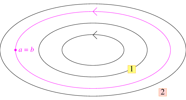
All methods based purely on the velocity field (such as finite-time Lyapunov exponents, curves of extremal attraction, transfer operators, or stable/unstable manifolds) fail in identifying this physical flow interface, even in these simple steady examples. If attempting to determine transport between the fluids, one numerical method which would work is to think of evolving the fluid density of each of the fluids according to an advection-diffusion (convection-diffusion) equation [35, 5, 36, 37, 23, 38] or other relevant dynamics [39, 36, 37, 40]. Rather than limiting attention to the fluid velocity and resulting Lagrangian trajectories, the trick would be to consider the two evolving fluid density fields. One might define the flow interface as a front of one of these density fields, and under the operation of advection and diffusion (assuming that there is a known way to parametrize the Péclet number which characterizes the strength of the diffusion), one might be able to computationally make progress on this issue. However, this will not help in obtaining a broader conceptual understanding of the process. How does the fluid interface evolve? Is it possible to characterize how ‘complicated’ it gets? How can the interchange of fluid be quantified? Is there an optimal velocity agitation to maximize cross-interface transport? Having a theory would give the ability to analyze questions such as these, with the longer term goal of being able to maximize or limit transport [41, 42, 43, 44, 45, 46, 47, 48] according to our wishes.
Studying interfaces between two miscible fluids is not new, and includes much recent work [36, 37, 49, 39, 50, 51, 40, 52]. The approach followed here, in which the Lagrangian particle evolution is directly used in conjunction with techniques inspired by dynamical systems theory, is however a novel approach, which moreover provides tools for answering the questions posed above. The key to proceeding is in determining how one might identify the flow interface under unsteady velocity agitations. It will be argued that the concept of a streakline is the most appropriate to use, under the condition that the velocity agitation is confined to a certain region. (The streaklines used here are not associated with stable/unstable manifolds, as might be the case if considering the interface between a fluid and a bluff body [53, 54, 55, 56].) Briefly, this is because if the agitation is confined to being downstream of in the top panel of Fig. 1, then the streakline passing through will demarcate the boundary between the two fluids, as fluids arriving from upstream on the two sides of are different.
This paper is organized as follows. Section II will develop the theory for the streaklines—the ‘nominal’ flow interfaces when the weak velocity agitations are considered—and their evolution with time. Explicit analytical expressions are obtained by utilizing dynamical systems methods, and are valid for general time-dependence in the velocity agitation, and also allow for compressibility in the fluid. Section III provides a validation of these expressions in comparison to numerical simulations of streaklines, in two examples which are loosely based on Fig. 1. Specifically, the first example considers the impact on the flow interface as a result of introducing flow in cross-channels (a so-called cross-channel micromixer [57, 58, 59, 60, 61, 5]), while the second concerns the impact on the ‘boundary’ of Kirchhoff’s elliptic vortex [62, 63, 64, 65, 66] due to weak external strain. In Section IV, a theory for quantifying the transport between the two fluids as a result of the agitation is developed. Of particular interest here is the question of ‘transport across what?’ since when the flow is unsteady, there is ambiguity in defining the fluid interface. If the interface is thought of in terms of a timeline (i.e., particles seeded on the interface, and evolved with time), since the timeline is a material surface, there can be no transport across it. Therefore, an appropriate way of defining a ‘nominal’ flow barrier, which respects the streakline ideas, needs to be formulated. An explicit approximation for the transport between the two fluids is obtained; this shall be useful in future work in, for example, determining forms of velocity agitations which maximize transport (as in the similar developments for heteroclinic situations [67, 46, 48, 47]). The theory is once again validated by numerical simulations of the same two examples in Section V. The second of these offers a novel way of examining the oft-studied problem of vortices in an external straining field [68, 69, 23, 38, 70, 71, 72, 73, 74]; here, the Lagrangian fluid interchange between the interior and exterior fluids caused by weak external strain is quantified. Finally, directions of future work are outlined in Section VI.
II Upstream and downstream streaklines
Consider a steady two-dimensional flow in which there is a persistent (one-dimensional) flow interface between two different miscible fluids. The persistence of this entity is annoying from the perspective of mixing the two fluids together, and hence the goal is to understand how an unsteady velocity agitation affects this flow interface, and how the resulting advective transport between the fluids can be quantified. Firstly, to introduce notation, consider the steady flow
| (1) |
Incompressibility is not assumed for the fluids, but is assumed to be smooth. Now, a flow interface that persists in the steady flow (1) must have no fluid velocity perpendicular to . Thus, the velocity is tangential to , which can be characterized as part of a streamline of the initial steady flow. Since the velocity is steady, this can be thought of as a streamline, streakline, or pathline, but as shall be seen shortly, when an unsteady velocity agitation is applied, thinking of the flow barrier as a streakline is the correct approach. Let be such a streakline. A velocity agitation will be applied to the part of which lies between the points and only, and this restricted part of shall be denoted . Thus, is a curve which starts at the upstream anchor point , and connects along the streamline emanating from and progressing to the downstream anchor point . Two generic situations are possible: (i) , in which case is an open curve, and (ii) , in which case is a closed curve. These two situations are exactly analogous to those shown in Fig. 1; however, there is no necessity for the streaklines to be as uniform as those pictured here. The streakline is the extension of along the streaklines passing through and ; it is clear that in the open case extends beyond . In the closed case, the streakline can be thought of as retracing the closed loop repeatedly, as will happen if dyed particles are continually ejected at .
There are two assumptions on the flow interface. The first is that be a simple (non self-intersecting) curve. The second—which is crucial—is that on . If at some points on , then will consist of parts of heteroclinic manifolds, and established theory for locating these [75, 4, 3], and the resulting transport time-periodic [68, 76, 77], aperiodic [78] or impulsive [79] situations, applies. Moreover, standard diagnostic tools such as finite-time Lyapunov exponents or curves of maximal attraction are viable candidates for numerically determining the flow barriers. Therefore, stagnation points will be explicitly precluded on ; it shall be non-heteroclinic.

The streakline is easily defined as a curve in , via a parametrization as shown in Fig. 2. Here is a solution to (1)—where the parameter can be thought of as time—which obeys and . The superscript is to be identified with ‘upstream,’ and with ‘downstream’ throughout this article. The restriction identifies , the part lying between and , to which the velocity agitation will be confined. If is closed, then the velocity agitation will occur throughout (the periodic repetition of , except at the anchor point . Indeed, is a periodic function of in this instance, but the restriction to acheived by setting implies that but that is the next instance in which reaches , which is of course . In either the open or closed situation, of interest is the fact that the upstream streakline emanating from is identical to the downstream streakline emanating from in this steady situation, and moreover these are each identical to .
In preparation for introducing time-dependence in the velocity, it pays to understand how the upstream streakline evolves with time. The time-variation of this upstream streakline can be quantified by the definition
| (2) | |||||
The above provides a parametrization of the upstream streakline at each fixed time instance , where the can be thought of as identifying a particle. The particle which is at the location at time is the one which passed through at time (i.e., a time prior to ). Note that the upstream streakline here is not restricted to , since the -values go beyond . This therefore incorporates parts of before (these are particles which will go through in the future), and beyond (these have gone through in the past) shown by the dashed curve in Fig. 2. The upstream streakline encapsulates all trajectories that will go through , in their entirety. Analogously, the downstream streakline
| (3) | |||||
identifies all particles which go through the downstream location at some time. For closed , since , the upstream and downstream streaklines coincide. Thus, in this case, it suffices to simply use one of the definitions.
The parametrization above—with being a fixed particle along the streakline and the time at which the streakline is being observed—shall be retained when the flow is subject to an unsteady velocity agitation in the form
| (4) |
The agitation velocity on shall be confined to be between and only. This shall specifically be stated as
| (5) |
For open this means that the unsteady agitation is zero up to (and including) the point , which enables the understanding that the continues to be at the interface of the two fluids, as they come in towards . Thus, continues to be an anchor point on the flow interface in forward time. Similarly, would be an anchor point on the interface in backward time. For closed , , and periodically traverses . Thus, once going ‘beyond’ on , one returns to points in which a velocity agitation continues to exist, and it cannot be ‘turned off’ as in the open situation. To enable an anchor point on the flow interface to continue to be defined under the agitation, it is necessary to fix the agitation to be zero at , which shall be the release point of the streakline. Moreover— in representing this as an agitation on a dominant steady flow—it shall be assumed that
where , and is smooth in . Note however that is otherwise arbitrary for the theory to follow: it may satisfy , possess aperiodic time-dependence, etc. Now, exactly analogous to the definitions of the steady upstream and downstream streaklines, the unsteady ones associated with (4) can be defined by
| (6) | |||||
and
| (7) | |||||
A mild technicality in comparison with the steady streakline definitions is the replacement of the by , which is any finite positive number. This because it is not possible to maintain control for all time for particles which have gone through the velocity agitation region, but this can only be accomplished for finite times, as large as required.

These streaklines at a fixed time are shown in Fig. 3, to be viewed in conjunction with the steady (non-agitated) streakline picture of Fig. 2. The steady of Fig. 3 is shown by the thick curves: it consists of the thick red curve upstream of , the thick dashed black curve between and (i.e., ), and the thick green curve downstream of . The unsteady upstream steakline is shown in red, and consists of a thick part which coincides with (upstream ), and then the extension which need not. Similarly, , shown in green, coincides with downstream of (shown by the thick green curve), while not necessarily so upstream of . As time progresses, (the thin portions of) will wiggle around due to the velocity agitation. They may even intersect in various ways. Since the upstream and downstream streaklines are not necessarily coincident, the previously clear flow interface between the two fluids has broken. Fluid arriving towards on the two sides of , and then subsequently advecting in forward time, are separated by the upstream streakline . On the other hand, fluid which is ‘separated’ by the part of downstream of is separated by in backward time. The intermingling of and results in fluid which was separated in backward time not being identical to the fluid which is separated in forward time. Transport is achieved between the two fluids as a result of this, and shall be explored in more detail in Section IV. At this point, the focus shall be on determining the time-varying locations of the upstream and downstream streaklines.
In preparation for stating the characterization of the unsteady streaklines, the notation
will be useful. Notice that rotates vectors by , and from Fig. 2,
| (8) |
is a unit normal vector to at the parametric location . The unsteady modifications to the upstream and downstream streaklines in this normal direction can now be quantified:
Theorem 1 (Upstream streakline)
For the proof, the reader is referred to Appendix A. The crux of this theorem is in characterizing the normal displacement from to a point on , as indicated by the arrow in Fig. 3. This is therefore given for by
| (11) |
if the tangential displacement is ignored 22 2 Ignoring the tangential displacement is reasonable in the sense that the streakline has as its parameter varying in precisely the tangential direction, and when plotting for a range of to obtain the streakline curve, any tangential displacement will be barely visible [75]. This is indeed reflected in the examples presented here. If needed, tangential displacements can be quantified [75], but this is unwieldy.. This allows for the streakline to be located and tracked theoretically to , since due to the presence of in the integral (10).
The prefactor in (10) simply ensures that the displacement is zero upstream of if is open, but if is closed, ‘upstream of ’ is once again in the velocity agitation region and thus the displacement incurred is not zero. The subtlety in the upper limit is because in the open situation, once a particle has gone beyond (i.e., beyond ), there is no longer any velocity agitation applying. Hence there will be no additional (leading-order) change in each particle’s position, and so will be set to as shown in Table 1. Before arriving at , it will be ; hence the expression . If is closed, when a particle approaches it has once again arrived at , and it will experience the velocity agitation once again as it repeatedly traverses a path which is close to . Hence the setting of . There is no necessity for to consist of a closed loop, however, since when a streakline arrives back to near , it will generically not be at . This streakline will then wrap around repeatedly. In computing the displacement of the streakline in the closed situation, the terms in (10) involving will therefore periodically repeat, but the presence of the general time-dependence in in (10) ensures that the normal displacement is not generally periodic in or .
If only interested in forward time, i.e., the time-varying curve which separates the two different fluids arriving at and progressing beyond, then the upstream streakline is what is needed. However, the downstream streakline is relevant to understanding the origins of the fluid which are separated beyond . The separating curve is the streakline passing through , i.e., the downstream streakline. As will be seen in Section IV, the downstream streakline also becomes important when attempting to quantify the transport across the (now broken) fluid interface. A similar quantification of the modification, in the direction normal to , of the downstream streakline is possible:
Theorem 2 (Downstream streakline)
The proof for Theorem 2 is similar to that of Theorem 1, and shall be skipped. The use of this theorem is the possibility of representing parametrically by
| (14) |
for . A point which is perhaps not obvious is that when drawn at a time , an upstream streakline may intersect a downstream streakline, in either a transverse or tangential fashion. This is because such intersections correspond to fluid particles which went through in the past, and will go through in the future. This is in constrast to ‘standard’ streakline approaches which might consider releasing particles from both points continuously in time, and viewing the resulting evolving curves forward in time; in this case, intersections are prohibited unless the streakline through has at some intermediate time gone through .
III Streakline validation
In this section, streaklines will be obtained by numerical simulation, and compared with the theoretical expressions of derived previously, in two examples: two fluids in a channel, and an anomalous fluid inside an elliptic vortex. These same examples will be examined subsequently, in Section V, in computing the associated fluid transport.
III.1 Two fluids in a microchannel

As the first example, consider two incompressible fluids travelling along a straight channel. At the microfluidic level, it is well-known that these will tend not to mix across their flow interface, and sloshing fluid in the direction normal to this interface via cross-channels is a standard strategy which is used [57, 58, 59, 60, 61, 5]. This interface is shown by the dashed curve in Fig. 4, which need not be centered since the volume flow rates of the upper and lower fluids need not be the same. For well-developed steady flow (with no flow in the cross-channels), fluid along the interface will at a constant speed, . The steady streakline is therefore . To account for the many possibilities which are available in the literature, a general geometry consisting of cross-channels shall be assumed. The th cross-channel is centered at the location , and is assumed to have width , where for consistency it is necessary that . In this case, , and the upstream point can be taken to be any point upstream of and the downstream point any point downstream of . Thus, and . Experimental evidence [60, 59, 61, 48] suggests that the flow in the cross-channels takes on a parabolic profile, which can be modeled by
| (15) |
for , where is a velocity scale representing the speed at the center of the cross-channel, is the frequency of fluid sloshing, and enables the specification of how the cross-channels are operating in relation to one another. For example, if all cross-channels are in phase, then , and if adjacent ones are exactly out of phase, then . Therefore, the geometry and velocity specification can account for very general cross-channel configurations. It is assumed that .
The observations , and are useful in computing the upstream streakline as given in (11). Thus, to leading-order
| (16) |
where, from (10),
| (17) |
(The subscript is used for ‘channel,’ to contrast with the vortex example to be presented subsequently.) For given parameter values, the integral above can be explicitly computed, thereby providing the time-variation of the upstream streakline via an explicit expression for this general geometry. To compare with numerics, choose a situation where , , and , with channels specified by , , and . Thus, the second cross-channel has a smaller maximum speed than the others, the fourth is triple the width of the others, and the fifth has a phase which is at odds with the exactly-out-of-phase nature of the other channels. Initially, is taken to be the fluid interface. Numerical simulations with red dye released at (upstream of velocity agitations) on the interface at time are shown in Fig. 5 at several instances in time. The black curves illustrate the instantaneous velocities in the cross directions, scaled so that they fit into this picture. It should be noted that beyond (the final point at which the velocity agitation applies with these parameter values, the streakline is not simply along . The curves in the streakline caused by the velocity agitations will be swept along, with no additional agitation. A video of the upstream streakline (i.e., unsteady fluid interface) evolution is provided with the Supplementary Materials.


In Fig. 6, the identical parameter and time values associated with the numerical streakline calculations were used, but now the theoretical leading-order upstream streakline (expressions (16) and (17)) is plotted. The agreement between Figs. 5 and 6 is excellent. One slight difference is that in the theoretical streakline as shown in Fig. 6, the streakline extends all the way across. This is because the theoretical streakline has been computed by considering fluid particles going through at all times in the past. In contrast, the numerical streaklines shown in Fig. 5 were obtained by synthetically releasing red dye at from time onwards. While making a decision of this sort is inevitable in a numerical simulation, the theoretical expressions enable the full streakline, associated with particles released at in the distant past, to be obtained.
To compare the differences in more detail, Fig. 7 shows the numerical simulations (red dots) and the explicit approximation (blue curve) in one plot, at the time corresponding to the last panel in Figs. 5 and 6. This is five times the period of the flow (allowing for the numerically simulated streakline to approach the right-end of the figure), and indeed it should be noted that the streakline must also be periodic in with exactly this period. In general, however, the theory of the previous section does not require such periodicity. The red dots are virtually on top of the blue curve, while it should be noted that is of moderate size. The error is further investigated in Fig. 8, in which the square-sum () error along the streakline, , between the numerical and explicit streaklines is computed at for different values of , and shown by the dots. The linear fit in the log-log plot indicates that the error goes as , which is consistent with the prediction of the theory.


III.2 Anomalous fluid in a vortex

For this example, the attitude adopted by Turner [72] of modeling the interaction of a coherent vortex with its surroundings (consisting possibly of many other vortices distant to it, and also the effect of boundaries) by using a weak external strain field is adopted. While it would be convenient to use a line or Gaussian vortex with circular streamlines (on which particles flow at a constant speed) as the base flow, the utility of the method will be illustrated by using the more complicated Kirchhoff’s classical elliptic vortex [62, 63, 64, 65, 66] as the prototype. In nondimensional coordinates in 2D, this has the flow given by
| (18) |
with , which consists of nested elliptical streamlines centered at the origin. Suppose there are two different fluids inside and outside the elliptic streamline defined by
as shown in Fig. 9, and take . Another rationalization for the choice of this particular streamline could be that it is associated with a critical angular momentum value as dictated by an outer flow [72], thereby defining the ‘boundary’ of the vortex; however, the ‘two-fluid’ paradigm as illustrated in Fig. 9 will be the main motivation which drives the analysis to follow. Before introducing an external strain field as an unsteady velocity agitation, a useful parametrization shall be presented. If is the standard polar angle, then the ellipse has a parametrization with being . So will be used instead of to identify location/particle along the streakline. Therefore
The rotation is anticlockwise around , and thus the relevant normal unit vector is
which points ‘inwards’ as shown in Fig. 9. If is the time variation as a particle traverses , then
and so the relationship between the time and the polar location is
| (19) |
where the choice when (i.e., at ) has been made.
Now, following a commonly modeled idea [68, 69, 23, 38, 70, 71, 72, 73, 74], suppose the vortex is placed in an unsteady strain field. Here, this is modeled by the inclusion of a weak unsteady velocity agitation added to (18), subject to the constraint that for all . Then, Theorem 1 gives the fact that the unsteady streakline at a location and time perturbs in the direction by an amount (see also Fig. 9). The subscript used here is for ‘vortex,’ to distinguish from that of the previous example. Thus, the - and -coordinates of the unsteady streakline to leading-order obey
| (20) |
and
| (21) |
The value of can be obtained from (10), with now identified with , and by recasting the integral with respect to the polar angle as opposed to using (19):
| (22) |
In obtaining (22), several factors such as the incompressibility of the flow in (18), and the rewriting using (19) of in the temporal argument of , have been used. There should be a term in (10) which multiplies the above expression (but has not been explicitly stated), where is any large number; this simply means that (29) is valid for any finite , but not for .
Next, the theoretical flow interface, as characterized by the unsteady streakline expression above, shall be verified for a particular choice of unsteady velocity agitation . Suppose that, conforming with for all ,
| (23) |
is chosen, where is small. This represents an agitation in the -direction which is modulated periodically in , but aperiodically in time. Thus, the expressions in (20) and (21) will be the expressions for the streakline, with error . The general expression (22) becomes in this situation
| (24) |
Numerical simulations of the streakline passing through are shown in Fig. 10, where , , with red dye is released from time onwards. To accentuate the variation displayed, the relatively large value of is used. It should be noted that as increases, the streaklines shown are not simple retracings and extensions of previous curves; the previous curves are themselves moving. The velocity agitation (23) considered here is purely in the -direction, and displays a transition at between two (almost) stationary states; this is displayed by the black dashed curve (scaled in the -direction to be visible in this plot). A movie of the streakline evolution is provided with the Supplementary Materials. As the streakline wraps around, in this case the inner parts of the streakline accummulate towards an almost elliptic trajectory. The analytical expressions given by (20), (21) and (22) are used to generate Fig. 11. By choosing the range of , the analytical streakline can be computed beyond the lead point of the figures in Fig. 10 (representing dye released from before ), and also backwards from the point (representing points which will go through in the future). However, in producing Fig. 11, a range which is approximately that displayed in Fig. 10 has been used to enable comparison. The agreement between the theoretical and numerical streaklines is good even at this value of . However, as the streakline wraps around, the analytical expression loses its ability to match the simulation. The reason for this is that in the analytical expression, the leading-order velocity on is what is being used, even as it wraps around. In reality, however, after wrapping around once, the streakline would have ventured into a different location. This is still -close which means the analytical expression is rigorous, but the error term, which is valid for in terms of the definition of the upstream streakline (6), now kicks in. In terms of , this means that the error can increase outside a domain . This fact is being displayed in Fig. 11, with the error clearly increasing at large . The matching between the curves when restricted to wrapping around just once is very good, and smaller values (not pictured), have greater accuracy (even for several wraps around). Furtunately, as shall be seen in Section IV, restricting to wrapping around less than once is sufficient in evaluating transport of fluid.


IV Transport quantification
Previous sections outlined theory and examples in determining the upstream and downstream streaklines under a velocity agitation. Before the agitation, these coincided, and ran along the flow interface between the two fluids. Thus, in that situation, there was no transport across the flow interface. The issue now is to attempt to quantify the transport ‘across the flow interface’ after the agitation. But what exactly is the flow interface after applying the agitation? Does it make sense to compute a flux across a stationary (Eulerian) curve? How can a flux in a Lagrangian sense be defined?
The difficulties here are familiar in a different situation: when the interface consisted of a coincident stable and unstable manifold (a so-called heteroclinic manifold) before perturbation. After the agitation, it would split into stable and unstable manifolds which are not coincident, and which moreover move with time. In this case, the concept of lobe dynamics [68, 76] can be applied when the agitation is time-periodic in a specific way, or for more general perturbations it is possible to define an instantaneous transport [78, 32]. However, the current situation is different: the original flow interface is not a heteroclinic manifold. Nevertheless, the ideas from [78, 32, 3] can be adapted to this situation.

Suppose that, before perturbation, the flow interface was unequivocally defined by , as shown in Fig. 2. Now, when the velocity agitation is included, at each time there will be an upstream streakline going through , and a downstream streakline going through , as shown in Fig. 3. Consider fluid arriving near to from upstream. The fluid on either side of the upstream streakline is different, and therefore will continue to be different as time progresses forward. In other words, the upstream streakline can be considered a flow interface between the two fluids in forward time. On the other hand, consider fluid on the two sides of the downstream streakline to downstream of . Had there been no velocity agitation, the downstream streakline would separate the two fluids as one progresses downstream from . But the presence of the velocity agitation means that this separation has been disturbed, and the relative positioning of the upstream and downstream streaklines, and their movement with time, affects the transfer of fluid. How can this transfer be assessed, bearing in mind that the streaklines shown in Fig. 3 are wiggling around with time, and may (or may not) intersect in various ways in the agitation region?
The trick to computing a transfer, specifically as an instantaneous flux of fluid, is to use the idea of a gate which was originally suggested by Poje and Haller [81] (and used elsewhere [82]) as a strategy for flux determination across numerically determined stable and unstable manfolds, but later adapted by Balasuriya to obtain a flux for a broken heteroclinic situation in time-aperiodic flows [78, 3]. Consider a time . Take a parameter value , and consider the point on , i.e., a point on the original steady streakline but within the agitation region. Draw a normal line to at this point, extending far enough out to intersect both the upstream and the downstream streakline . The intersections occur at the points and respectively, and these must be near to . This construction is shown in Fig. 12, based on the streakline configuration in Fig. 3. This line between and is the gate . Now define the pseudo-streakline to be the three connected curves (i) the upstream streakline until it hits , (ii) the gate , and (iii) the downstream streakline continuing on from that point. This is the collection of solid curves in Fig. 12.

The pseudo-streakline is a method for trying to identify a ‘nominal’ flow interface, in this unsteady instance in which there actually is no impermeable barrier (since transport occurs between the two fluids). Moreover, since it is defined using segments of , it specifically incorporates the Lagrangian nature of the flow, which is essential in determining transport. To see how transport can be quantified, refer to Fig. 13, which retains the pseudo-streakline as constructed in Fig. 12. Suppose the fluid upstream of is labeled and ; the upstream streakline separates these two fluids in forwards time. On the other hand, suppose the fluids downstream of were labeled and . In the absence of a velocity agitation, the upstream and downstream streaklines would coincide, and lie exactly along . Thus, fluid from region will go to , and to , with no intermingling; is in this steady instance an unequivocal flow interface. The agitation has broken this interface into two entities (the upstreak and downstream streaklines), which are both moving with time, leading to difficulty in defining an interface. The pseudo-streakline incorporates information from both these entities. The transport of fluid across the pseudo-streakline will help define a fluid transport, as follows.
The wish is to quantify how fluid transfers to , and how transfers to ; these were both zero when there was no unsteady agitation. Now, examining Fig. 13, the transfer of fluid to , across the pseudo-streakline, at this instance in time, only occurs by fluid crossing . This is because portions of which are also part of the pseudo-streakline cannot be crossed since these are flow separators. Therefore, the transport of fluid across the gate explicitly characterizes the transfer of fluid from to in the situation pictured. In this case, note that the transfer, in relation to the unperturbed , is in the direction of the normal vector across . If the upstream and downstream streaklines were positioned in the opposite orientation (i.e., was above along in Fig. 13), then the transfer of fluid across the pseudo-streakline would be associated with fluid going to . This is in the direction across . In either case, this is clearly an exchange of fluid.
Suppose the gate is parametrized in terms of the arclength along it. Let be the normal component of the full velocity field across the gate at each location, i.e., the component of the velocity in the direction of . Then, the instantaneous flux across the pseudo-streakline is by definition
| (25) |
Note that the velocity normal to in general includes contributions from both the steady () and unsteady () terms, and moreover is not the same value at all points on . The above is a explicitly a flux in the sense that it is an area of fluid per unit time which crosses the pseudo-streakline instantaneously. If in the positive direction (as in Fig. 13), will be positive. In the upstream/downstream streaklines have the opposite orientation along the normal vector, then it will be negative. When thinking of a time-varying flux, it is best to think of as fixed, corresponding to fixing the location of the gate. As time varies, however, will change, since the locations will vary along the normal vector. At some instances in time, and can interchange their relative positions. If so, these points will ‘go through each other’ on the gate, at that instance in time. The instantaneous flux at this time will be zero. However, once they have gone through one another, there will be flux in the opposite direction. The continuing time-variation of will indicate how fluid continued to go back and forth.
If were closed, the pseudo-streakline would be a closed curve consisting of parts of the upstream and downstream streaklines going through , capped by a gate. (Think of glueing to in Figs. 13 and 12, and throwing away the parts upstream of and downstream of .) This is a nominal flow barrier between the interior and exterior fluids. Moreover, the upstream and downstream streaklines must connect smoothly at , since adjacent points are associated with dye particles which went though a moment ago (on the upstream streakline), and which will go through in a moment (on the downstream streakline). Since remains indubitably on the flow interface, one might consider that the streakline (upstream and downstream) passing through is the flow interface. However, in general these do not coincide as one wraps around , and there will have to be a gate of finite size which connects them at the location . Transport between the interior and exterior fluids—crossing the nominal flow interface—will in general occur by fluid crossing the gate.
Thus in either the open or closed situation, (25) gives the instananeous flux across the nominal flow interface. A simple leading-order expression for is possible:
Theorem 3 (Instantaneous transport)
Consider a pseudo-streakline at time as defined in Fig. 13, with the gate drawn at the location . The instantaneous flux across the pseudo-streakline is
| (26) |
where
| (27) |
For the proof, the reader is referred to Appendix B. The power of Theorem 3 is that, unlike in the definition (25), the instantaneous flux can be represented in terms of known quantities from the steady flow, and the unsteady velocity. Unsteady trajectories (and in particular the unsteady streaklines) are not needed.
A question that might arise is the effect of the location of the gate on the transport quantification. This dependence occurs precisely because a genuine flow interface does not exist after velocity agitation, and therefore a choice needs to be made in demarcating such a interface. This is almost exactly the same issue pondered by Rom-Kedar and collaborators [68, 76] in the freedom of deciding on a ‘pseudo-separatrix’ associated with transport across a heteroclinic manifold in an specifically time-periodic vortical flow. While the current problem is neither heteroclinic nor time-periodic, having to make such a choice is inevitable in the absence of a genuine flow interface. However, if the flow is incompressible, it turns out that this freedom for choosing the location of the gate is actually a spurious freedom. This is because if one takes (27) under the hypothesis that , it is clear that and do not appear independently in the instantaneous flux , but together in the combination . Thus, a shifting of (corresponding to choosing a different location for the gate) merely shifts the time-variation of the flux.
V Transport validation
The two examples examined in Section III are now re-examined. Here, the focus is on determining the advective transport resulting from the interface streakline separating into upstream and downstream streaklines, as outlined in the previous section.
V.1 Two fluids in a microchannel


Consider two fluids in a microchannel, with exactly the velocity agitation and parameter values as used in Section III. Suppose the gate is to be drawn at the value , i.e., at the choice . To numerically simulate the upstream pseudo-streakline at some instance in time , it is therefore necessary to release particles from at times prior to , and allow the streakline to evolve until it intersects a vertical line drawn at . To plot the downstream streakline at the same instance in time, particles must be released synthetically from , which was unspecified in Section III beyond the fact that it must be downstream of . Here, let us take to have the gate be symmetrically between and . However, particles need to be released from after the time , and evolved backwards in time until the gate is intersected. This means that, in general, using numerical simulations to determine the pseudo-streakline—which contains simultaneous snapshots of the upstream and the downstream streakline, ending exactly on the gate—may not be easy. It may not be clear at what instance in time to release particles at and at such that the streakline evolving from these points precisely intersects the gate at the same specified instance in time . Fortunately, for this particular example, since the velocity agitation is in the -direction, and the steady velocity is a constant in the -direction, this can be determined.
Fig. 14 shows the pseudo-streaklines obtained by this process at four different times. At , the flow through the gate indicates that fluid will get transported from the lower to the upper fluid. Since this is in the direction of , this represents a positive instantaneous flux. At , the flux is negative (fluid transports from the upper to the lower fluid through the gate), while it is positive once again at . There is a value between these, near , at which the upstream and downstream streaklines interchange their relative positions on the gate. This is shown in the third panel of Fig. 14; the red and green curves meet on the gate. This is a situation at which the instantaneous flux is zero. As time progresses, repeated interchanges of relative positioning along the gate implies that fluid sloshes back and forth across the gate (and hence across the pseudo-streakline), causing advective transport between the two fluids. The flux (25) in this case is easily obtained by multiplying the length of the gate by the horizontal speed , since the normal velocity to the gate at all points on the gate is the same value. In doing this calculation, the length of the gate should be considered a signed quantity, to reflect the correct direction of transport.


Next, this shall be compared to the analytical expression in Theorem 3. Before writing the instantaneous flux expression for this specific configuration, it can be written for a general channel configuration as described in Section III by
| (28) |
where , and denotes the location of the gate. For a fixed , it is clear that the flux is periodic in with period . This is easily computed for the given parameter values. Now, for the specific channel configuration and parameter values as examined in Section III, the analytical expression is compared with that obtained by the direct numerical simulations inserted into the flux definition (25) in Fig. 15. The top panel shows , the particular value used in Section III, with the red being the numerics and the blue the analytics. The curves are indistinguishable. The lower panel shows the comparison performed now with (but everything else kept identical), showing that indeed the theory loses predictive ability when the agitation is comparable in size to the main flow. Having said that, the theorerical blue curve, obtained using perturbative methods in , still does an excellent job of following the trend of the flux, even for non-small velocity agitations.
V.2 Anomalous fluid in a vortex
Unlike in the previous example, the flow on is not of a constant speed, is curved, and the velocity agitation is not always perpendicular to . Determining the pseudo-streakline at a general time will therefore be more complicated. Take as before, and let be the identical point but after the vortical flow has taken the particle released from one round around the vortex. Thus, when using instead of as a parameter, corresponds to and to . Choose the gate to be drawn at . Since the flow at is in the -direction, the gate occurs along the -axis at this point. Note that points into the vortex; positive instantaneous flux will therefore entrain exterior fluid into the fluid in the interior, whereas negative flux indicates that at that instance in time the interior fluid is escaping.
The fact that the gate is chosen such that the pseudo-streakline consists of parts of streaklines which wrap around the vortex less than once is immediately comforting. This avoids having to deal with accummulated errors when streaklines wrap around more than once, as seen in Section III.
Numerically determining the pseudo-streakline at an instance in time entails first releasing particles from at some time instance in the past, and then allowing the upstream streakline to evolve until it crosses the gate on the -axis. The time one needs to start releasing particles is therefore only implicitly defined, which lends some difficulty in the computation. Similarly, particles need to be released from at some time instance in the future of , and evolved backwards in time until is intersected at exactly time . In performing numerical simulations, an overestimate for the time before for the upstream streakline (or after for the downstream) is estimated first to be from (19), since in the absence of a velocity agitation the time would be exactly . Then the upstream streakline is evolved up to this time beyond , and portions which extrude across are then clipped. By following the same idea, the downstream streakline can be obtained, and the gate drawn in between these. Using exactly the parameter values as in Section III, the pseudo-streaklines were obtained using this procedure at different times , and are pictured in Fig. 16 by the solid curves. The dashed curves are obtained from the analytical approximation (24) and the corresponding expression (not shown) for the downstream streakline. The instantaneous flux is going out of the vortex at all instances pictured, with a large value at , smaller at , and very small at . Numerical simulations at many other time values (not shown) indicate that the flux is always negative (i.e., outward), but becomes vanishingly small as gets large. Can an insight to this be obtained from the theoretical transport measure?
In calculating this, the first observation is that the downstream quantity for a general incompressible velocity agitation is almost the same as (22), excepting for the absence of the leading negative sign, and the fact that the limits are from to . Thus, the instantaneous flux function becomes
| (29) |
For the specific velocity perturbation considered in Section III, and with the gate chosen to be at , the instantaneous flux becomes
| (30) |
This is shown by the blue curve in the top panel of Fig. 17 for the same parameter values used for the numerical simulation. The theoretical flux is always negative, has a time-dependence which is symmetric about (reflecting the term chosen in the velocity agitation), and decays to zero. The implication is that the fluid which was in the interior of the elliptic vortex continues to leak out at all times, though the leakage is largest near and becomes vanishingly small as gets large. This will be visible as a tendril or filament of the inner fluid escaping to the outer one, with the tendril wrapping around in the anti-clockwise direction. It is interesting that this new approach reveals exactly the qualitative behavior that is well-documented for vortices in external shear flows [38, 6, 73]. From the mixing perspective, diffusion would then act on the tendril, causing the inner fluid to becomes dispersed in the outer one. The effect of diffusion is not explicit in the theory here, which focusses specifically on the advective (Lagrangian) flow. However, in reality this advective process promotes fluid mixing through advection-driven diffusion.
The red curve in Fig. 17 is obtained from numerical simulations, using the definition (25), for the same parameter values as the theoretical blue curve. At this relatively high value of , there is some difference between the curves. Taking smaller values would make the curves approach one another.


A minor point which must be made is the connection to imcompressibility, which is satisfied for the velocity conditions chosen in this example. Does the fact that there is a flux exiting the vortex for all time contradict incompressibility? The answer is no, since the closed pseodo-streakline—the purported flow interface under the unsteady conditions—compensates for the expelled fluid by becoming smaller. This is indeed visible by comparing the areas enclosed within the closed pseudo-streaklines in Fig. 16; these get smaller as increases. Indeed, the rate of change of the area enclosed by the pseudo-streakline is precisely the definition of the instantaneous flux, when is closed.

VI Concluding remarks
The concepts of stable and unstable manifolds—and various finite-time analogues such as finite-time Lyapunov exponent ridges [12, 13, 14, 15, 16, 17, 18, 33], curves of extremal attraction/repulsion [1, 7, 9, 10, 11], partitions based on Perron-Frobenius operators [19, 20, 21], time-clipped manifolds [22, 32], fronts associated with averaged flow quantities [29, 30] and other Lagrangian Coherent Structure type approaches [24, 25, 26, 27, 28]—are important in demarcating flow barriers in single phase unsteady flows. Here, the focus is on two-phase flows, in which such entities derived purely by examining the velocity field do not distinguish the flow barrier. In the steady, as-yet-unmixed situation, the flow barrier is the interface between the two fluids, which is identified physically as opposed to from characteristics of the fluid velocity. This article has focussed on determining the flow interface, and the transport across it, when an unsteady velocity agitation is introduced. The relevance of streaklines has been highlighted, and their usage in defining a nominal interface (a pseudo-streakline), and quantifying an instantaneous transport across this has been elucidated. Under the condition that the velocity agitation is weak (i.e., has speeds significantly smaller than that of the base steady velocities), a theory for determining the streaklines, and the transport flux, has been developed. Validations of the method in comparison to numerically computed streaklines was performed for the open (two fluids flowing along a channel) and closed (a blob of one fluid inside a vortex) flow interfaces situations.
The method for quantifying the transport across the flow interface developed in this paper depends on the velocity agitation being small in comparison to the base flow, which is steady. However, the method does not require incompressibility, or a particular form of time-dependence, and is thus fairly general. Indeed, it is likely that recent work [79] which characterizes the effect of an impulsive velocity (such as obtained by tapping a fluidic device, say) on stable/unstable manifolds, can be modified to determine the streaklines and transport associated with a non-heteroclinic flow interface, consonant for example with the impulsively strained vortex numerics of [73].
The presence of a theoretical approximation for the transport offers scope in being able to optimize it. Such has been done in the case where the flow barrier was a heteroclinic manifold (coincident stable and unstable manifold) in the situation where a sinusoidally varying velocity agitation was applied [67, 46, 47, 48]. Given that the transport expression (27) obtained in this non-heteroclinic instance shares some similarities with the heteroclinic theory of [67, 46, 47, 48], there is obvious scope in being able to adapt those ideas to this situation. Since there are also analytical expressions (11) and (14) for the streaklines, another possibility is being able to quantify how complicated these entities get due to advection, as a measure of eventual diffusive transport. There is considerable evidence of the presence of an optimal frequency of a velocity agitation in order to maximize mixing [48, 83, 84, 85, 86, 87, 88, 89, 90, 91]; would it be possible to determine this in, for example, configurations such as that of the channel examined here? Alternatively, can one obtain insight into the best positioning of cross-channels to effect the best mixing across the flow interface? Questions such as these are under investigation, and will be reported on in follow-up work.
It is interesting that streaklines have also been suggested as having importance in evaluating transport, independently by Karrasch in a recently accepted article [92] discovered by the author just before initial submission of the present paper. The differential topology and donating region viewpoints of that article [92] do not have an obvious connection to the present paper, which focusses on fluid interchange between two miscible fluids across their interface. Nevertheless, further investigation of a possible relationship will be pursued.
The approach presented here offers a different viewpoint on the oft-examined vortex-in-an-external-strain problem [68, 69, 23, 38, 70, 71, 72, 73, 66, 65], in the sense that it permits a direct computation of the fluid flux into, or out of, the vortex as a function of time, for a given weak external strain field. In this sense, it captures Lagrangian transport, as opposed to standard methods which, for example, picture the time evolution of the frozen-time (Eulerian) vorticity field [73, 72]. There are of course connections between the Lagrangian and Eulerian viewpoints, but in cases where the transport is important, the current approach may provide new insights.
The closed flow interface situation appears to be of particular interest in modeling how a blob of fluid (an oil/pollutant/nutrient/plankton/chemical patch) which is placed in an anomalous fluid mixes in with its surroundings. Once again, ‘standard’ methods for detecting coherent structure boundaries directly from the velocity field are not necessarily applicable, since the flow interface is a physical boundary between two fluids as opposed to an entity derivable from the velocity field. The methods outlined in this article are a first step towards understanding the Lagrangian transport associated with this from a theoretical perspective. The trick is trying to identifying the flow interface in the presence of an unsteady velocity, which can be done here if there is an anchor point on the interface at which the unsteady component of the velocity is zero. If not, there is a difficulty in deciding where to release particles for the streakline determination. How one might figure out the pseudo-streakline (i.e., the relevant unsteady flow interface) when there is no such anchor point is not clear. Note that the process of evolving particles on the closed steady flow interface (i.e., examining the timeline) is not effective in assessing transport, since this closed loop simply remains a closed loop under unsteady velocity agitations, and therefore a transport between the interior and exterior across this is zero. This is of course true for any material curve, which precludes their usage for transport assessment. A nominal flow interface across which there is transport needs to be enunciated. The ability to do so using streaklines when there is at least one anchor point, as outlined here, can hopefully be build on, in the situation of weak strain which is never zero on the interface.
Appendix A Proof of Theorem 1 [Upstream streakline]
The proof here is in the spirit of the proof of Theorem 2.1 in [75], in which an unstable manifold’s displacement is characterized. However, this situation is different, since it is the upstream streakline that is required. Imagine fixing the time , and also the particle in this time-slice which is at the location in the steady flow (1). Due to the action of the unsteady velocity agitation , this particle will be at a nearby location, away, at a location . Thinking of as fixed, but with as the time-variable, define
| (31) |
From (2), it is clear that , the steady streakline at location ; this passed through a time prior to . For the unsteady flow streakline as defined through (6), represents the location of the same particle, and thus is the difference occurring as the result of including . This difference is since is , and then so is . Note moreover that
| (32) |
is the projection of the displacement of the streakline in the direction normal to at . Hence, the goal is to determine in terms of known quantities from the steady flow. To do this, it is necessary to differentiate (31) with respect to at fixed . Fortunately, it turns out that this part of the calculation is identical to that in the proof of Theorem 2.1 in [75], and hence by inspection of equation (3.6) of [75] it is possible to write
| (33) | |||||
where terms have been discarded. Next, (33) will be multiplied by the integrating factor
and integrated from to . Before proceeding, these limits will require some explanation. The lower limit arises since when inserted into (31) this yields
by using the streakline property (6). Intuitively, this is because the particle from the steady streakline, and that from the unsteady streakline, share the property that they both emanated from the point . Next, consider the upper limit . If is open, using Table 1 in the situation where (i.e., the streakline has not yet reached ), then . Inserting this will give , which according to (32) is the correct entity sought in the time-slice . If, however, the streakline is beyond , it no longer experiences a velocity agitation. That is, for . In this case the upper limit becomes , thereby switching off the term when it is not present. On the other hand, if is closed, Table 1 implies that directly, leading to the quantity . As the streakline repeatedly traverses an -close path to , it continually accumulates modifications due to the velocity agitation. Thus, multiplying (33) by the integrating factor and integrating from to yields
| (34) |
Next, a change of variables is applied, and the integral above becomes exactly (10). However, there is an additional prefactor in (10). This simply ‘turns on’ the function for values above (all the way up to , where can be large). To understand this, consider first open , in which case according to Table 1, . If , the understanding of the streakline, according to (6) would be points which in the future pass through . Since there is no velocity agitation before particles reach , there is no correction to the steady streakline in this case. Hence, the correction term, encoded in , must be set to zero if , which is what is accomplished by the prefactor. Next, if is closed, particles which arrive at are already arriving from a region in which the velocity agitation applies, and thus will incur displacements from the steady streakline. Therefore, should not be set to zero for values of , which is accomplished by setting . (Recall that the definitions for the upstream (6) and downstream (7) streaklines were only legitimate for , for any finite value.) This completes the derivation of (10). The interpretation (11), as being the projection in the normal direction to , arises because of (32).
Appendix B Proof of Theorem 3 [Instantaneous transport]
The proof is based on two observations. First, the displacement from the downstream to the upstream streakline, measured along the gate, is from Theorems 1 and 2 simply to leading-order. If this is positive, it means that the upstream streakline is situated in a positive direction in comparison to the downstream one when considering the direction along . This enables the determination of whether the gate provides a channel for instantaneous flux from fluid to (if positive), or from to (if negative), as is clear from Fig. 13. Second, the fluid velocity at all points on , in the normal direction, is to leading-order . This is because in the absence of a velocity agitation the velocity at , on , is , and points normal to , and moreover both and the unsteady velocity agitation have size . Multiplying the velocity across by the length of therefore gives the instantaneous flux across it; to leading order this is therefore . Thus,
However, in this situation, and so and , whether is open
or closed. Moreover, by taking large, it is clear that the indicator function appearing outside the integrals in
(10) and (13) is always unity. Therefore, has an
integral from to , whereas has negative an integral from to . Since the integrand is
identical, this simply transforms to an integral from to , which gives the expression (27).
Acknowledgements.
Support from the Australian Research Council through Future Fellowship grant FT130100484 is gratefully acknowledged.References
- [1] G. Haller, Annu. Rev. Fluid Mech. 47, 137 (2015).
- [2] T. Peacock, G. Froyland, and G. Haller, Chaos 25, 087201 (2015).
- [3] S. Balasuriya, Melnikov methods for barriers and transport in unsteady flows, SIAM Series on Mathematical Modeling and Computation (SIAM Press, in press, 2016).
- [4] S. Balasuriya, in Ergodic Theory, Open Dynamics and Structures (Springer, 2014) Chap. 1, pp. 1–30.
- [5] S. Balasuriya, J. Micromech. Microeng. 25, 094005 (2015a).
- [6] S. Balasuriya and C. Jones, Nonlin. Proc. Geophys. 8, 241 (2001).
- [7] D. Kelley, M. Allshouse, and N. Ouellette, Phys. Rev. E 88, 013017 (2013).
- [8] J. Guckenheimer and P. Holmes, Nonlinear Oscillations, Dynamical Systems and Bifurcations of Vector Fields (Springer, New York, 1983).
- [9] G. Haller and G.-C. Yuan, Phys. D 147, 352 (2000).
- [10] D. Karrasch, M. Farazmand, and G. Haller, J. Comput. Dyn. 2, 83 (2015).
- [11] F. Onu, F. Kuhn, and G. Haller, J. Comput. Sci. 7, 26 (2015).
- [12] S. Shadden, F. Lekien, and J. Marsden, Phys. D 212, 271 (2005).
- [13] G. He, C. Pan, L. feng, Q. Gao, and J. Wang, J. Fluid Mech. 792, 274 (2016).
- [14] H. Huntley, B. Lipphardt, G. Jacobs, and A. Kirwan, J. Geophys. Res. Oceans 120, 6622 (2015).
- [15] D. Nelson and G. Jacobs, J. Comput. Phys. 295, 65 (2015).
- [16] P. Johnson and C. Meneveau, Phys. Fluids 27, 085110 (2015).
- [17] A. BozorgMagham and S. Ross, Commun. Nonlin. Sci. Numer. Simu. 22, 964 (2015).
- [18] M. Branicki and S. Wiggins, Nonlin. Proc. Geophys. 17, 1 (2010).
- [19] G. Froyland and K. Padberg, Phys. D 238, 1507 (2009).
- [20] G. Froyland, K. Padberg, M. England, and A. Treguier, Phys. Rev. Lett. 98, 224503 (2007).
- [21] G. Froyland, N. Santitissadeekorn, and A. Monahan, Chaos 20, 043116 (2010).
- [22] S. Balasuriya, J. Nonlin. Sci. , in press (2016b).
- [23] D. del Castillo Negrete, Phys. Fluids 10, 576 (1998).
- [24] M. Allshouse and J.-L. Thiffeault, Phys. D 241, 95 (2012).
- [25] R. Mundel, E. Fredj, H. Gildor, and V. Rom-Kedar, Phys. Fluids 26, 126602 (2014).
- [26] T. Ma, N. Ouellette, and E. Bollt, Chaos 26, 023112 (2016).
- [27] T. Ma and E. Bollt, SIAM J. Appl. Dyn. Sys. 13, 1106 (2014).
- [28] M. Budis̆ić and J.-L. Thiffeault, Chaos 25, 087407 (2015).
- [29] I. Mezić, S. Loire, V. Fonoberov, and P. Hogan, Science 330, 486 (2010).
- [30] Z. Levnajić and I. Mezić, Chaos 20, 033114 (2010).
- [31] M. Budis̆ić and I. Mezić, Phys. D 241, 1255 (2012).
- [32] S. Balasuriya, Phys. Fluids 27, 052005 (2015b).
- [33] S. Raben, S. Ross, and P. Vlachos, Experiments in Fluids 55, 1824 (2014).
- [34] Local maxima of the speed are defined by Haller as ‘parabolic Lagrangian Coherent Structures,’ for which a theory has been developed [1].
- [35] J.-L. Thiffeault, Nonlinearity 84, R1 (2012).
- [36] B. Guo, Z. Zheng, M. Celia, and H. Stone, Phys. Fluids 28, 022107 (2016).
- [37] Z. Zheng, L. Rongy, and H. Stone, Phys. Fluids 27, 062105 (2015).
- [38] P. Meunier and E. Villermaux, J. Fluid Mech. 476, 213 (2003).
- [39] J. Fernandez, P. Kurowski, P. Petitjeans, and E. Meiburg, J. Fluid Mech. 451, 239 (2002).
- [40] R. Camassa, Z. Lin, R. McLaughlin, L. Mertens, C. Tzou, J. Walsh, and B. White, J. Fluid Mech. 790, 71 (2016).
- [41] G. Mathew, I. Mezić, S. Grivopoulos, U. Vaidya, and L. Petzold, J. Fluid Mech. 580, 261 (2007).
- [42] Z. Lin, J.-L. Thiffeault, and C. Doering, J. Fluid Mech. 675, 465 (2011).
- [43] L. Cortelezzi, A. Adrover, and M. Giona, J. Fluid Mech. 597, 199 (2008).
- [44] A. Vikhansky, Chem. Engin. Sci. 57, 2719 (2002).
- [45] Z. Lin, E. Lunasin, A. Novikov, A. Mazzucato, and C. Doering, J. Math. Phys. 53, 115611 (2012).
- [46] S. Balasuriya, Phys. Fluids 17, 118103 (2005a).
- [47] S. Balasuriya and M. Finn, Phys. Rev. Lett. 108, 244503 (2012).
- [48] S. Balasuriya, Phys. Rev. Lett. 105, 064501 (2010).
- [49] M. Sussman, P. Smereka, and S. Osher, J. Comput. Phys. 114, 146 (1994).
- [50] R. Lynden-Bell, J. Kohanoff, and M. D. Popolo, Faraday Discussions 129, 57 (2005).
- [51] Y. Young, H. Tufo, A. Dubey, and R. Rosner, J. Fluid Mech. 447, 377 (2001).
- [52] K. Sahu, J. Fluid Mech. 789, 830 (2016).
- [53] P. Roca, A. Cammilleri, T. Duriez, L. Mathelin, and G. Artana, Phys. Fluids 26, 047102 (2014).
- [54] K. Shariff, T. Pulliam, and J. Ottino, “A dynamical systems analysis of kinematics in the time-periodic wake of a circular cylinder,” (American Mathematical Society, 1991) pp. 613–646.
- [55] E. Ziemniak, C. Jung, and T. Tél, Phys. D 76, 123 (1994).
- [56] M. Alam, W. Liu, and G. Haller, Phys. Fluids 18, 043601 (2006).
- [57] F. Bottausci, I. Mezić, C. Meinhart, and C. Cardonne, Proc. Trans. R. Soc. Lond. A 362, 1001 (2004).
- [58] F. Bottausci, C. Cardonne, C. Meinhart, and I. Mezić, Lab Chip 7, 396 (2007).
- [59] X. Niu, L. Liu, W. Wen, and P. Sheng, Appl. Phys. Lett. 88, 153508 (2006a).
- [60] P. Tabeling, M. Chabart, A. Dodge, C. Jullien, and F. Okkels, Phil. Trans. R. Soc. Lond. A 362, 987 (2004).
- [61] Y.-K. Lee, C. Shih, P. Tabeling, and C.-M. Ho, J. Fluid Mech. 575, 425 (2007).
- [62] G. Kirchhoff, Vorlesungen über Mathematische Physik, Vol. 1 (Teubner, Leipzig, 1876).
- [63] C. Y. Wang, Annu. Rev. Fluid Mech. 23, 159 (1991).
- [64] T. Mitchell and L. Rossi, Phys. Fluids 20, 054103 (2008).
- [65] L. Friedland, Phys. Rev. E 59, 4106 (1999).
- [66] V. Meleshko and G. van Heijst, J. Fluid Mech. 272, 157 (1994).
- [67] S. Balasuriya, Phys. D 202, 155 (2005b).
- [68] V. Rom-Kedar, A. Leonard, and S. Wiggins, J. Fluid Mech. 214, 347 (1990).
- [69] S. Kida, J. Phys. Soc. Japan 50, 3517 (1981).
- [70] T. Leweke, S. L. Dizes, and C. Williamson, Annu. Rev. Fluid Mech. 48, 507 (2016).
- [71] S. Mula and C. Tinney, J. Fluid Mech. 769, 570 (2015).
- [72] M. Turner, Phys. Fluids 26, 116603 (2014).
- [73] A. Bassom and A. Gilbert, J. Fluid Mech. 398, 245 (1999).
- [74] V. Zhmur, E. Ryzhov, and K. Koshel, J. Marine Res. 69, 435 (2011).
- [75] S. Balasuriya, SIAM J. Appl. Dyn. Sys. 10, 1100 (2011).
- [76] S. Wiggins, Chaotic Transport in Dynamical Systems (Springer-Verlag, New York, 1992).
- [77] S. Balasuriya, SIAM J. Appl. Dyn. Sys. 4, 282 (2005c).
- [78] S. Balasuriya, Nonlinearity 19, 2775 (2006).
- [79] S. Balasuriya, , submitted (2016c).
- [80] Ignoring the tangential displacement is reasonable in the sense that the streakline has as its parameter varying in precisely the tangential direction, and when plotting for a range of to obtain the streakline curve, any tangential displacement will be barely visible [75]. This is indeed reflected in the examples presented here. If needed, tangential displacements can be quantified [75], but this is unwieldy.
- [81] A. Poje and G. Haller, J. Phys. Oceanography 29, 1649 (1999).
- [82] P. Miller, C. Jones, A. Rogerson, and L. Pratt, Phys. D 110, 105 (1997).
- [83] L.-M. Fu, R.-J. Yang, C.-H. Lin, and Y.-S. Chien, Electrophoresis 5, 1814 (2005).
- [84] A. Rodrigo, R. Rodrigues, N. Formiga, and J. Mota, Chem. Eng. Comm. 193, 743 (2006).
- [85] S. Shin, I. Kang, and Y.-K. Cho, J. Micromech. Microeng. 15, 455 (2005).
- [86] Y. Wang, J. Zhe, B. Chung, and P. Dutta, Microfluid Nanofluid 4, 375 (2008).
- [87] C. Lim, Y. Lam, and C. Yang, Biomicrofluidics 4, 014101 (2010).
- [88] S. Wang, Z. Jiao, X. Huang, C. Yang, and N. Nguyen, Microfluid Nanofluid 6, 847 (2009).
- [89] H. Song, Z. Cai, H. Noh, and D. Bennett, Lab Chip 10, 734 (2010).
- [90] H. Suzuki, C.-M. Ho, and N. Kasagi, J. Microelectromechanical Sys. 13, 779 (2004).
- [91] X. Niu, L. Liu, W. Wen, and P. Sheng, Appl. Phys. Lett. 88, 153508 (2006b).
- [92] D. Karrasch, SIAM J. Appl. Math. , accepted (2016).