Memory Dependent Growth in Sublinear Volterra Differential EquationsThanks: Denis Patterson is supported by the Government of Ireland Postgraduate Scholarship Scheme operated by the Irish Research Council under the project GOIPG/2013/402.

We investigate explicit memory dependence in the asymptotic growth rates of positive solutions of the following scalar Volterra integro-differential equation

where $f$ is a positive sublinear function (i.e. $\lim_{x\to\infty}f(x)/x=0$) and $\mu$ is a non–negative Borel measure. The relevant existence and uniqueness theory regarding equations of the form (1.1) is well known and guarantees a unique solution $x\in C(\mathbb{R}^{+};(0,\infty))$ in the framework of this article [10, Corollary 12.3.2], with the convention that $\mathbb{R}^{+}:=[0,\infty)$. By defining the function

it follows that (1.1) is equivalent to

We also study the asymptotic behaviour of the perturbed Volterra equation

As with the unperturbed equation, it is useful to consider an integral form of (1.4), and by defining

it follows that (1.4) can be written in integral form as

In [6], with $\mu$ a finite measure, we demonstrate that when $f$ is sublinear and asymptotically increasing, the solution of (1.1) obeys $\lim_{t\to\infty}F(x(t))/t=\int_{[0,\infty)}\mu(ds)<\infty,$ where

In other words, the structure of the memory does not affect the asymptotic growth rate of the solution of (1.1) when the total measure is finite: indeed, the entire mass of $\mu$ could be concentrated at $0$, because the ordinary differential equation $y^{\prime}(t)=\int_{[0,\infty)}\mu(ds)\cdot f(y(t))$ for $t\geq 0$ also obeys $F(y(t))/t\to\int_{[0,\infty)}\mu(ds)$ as $t\to\infty$. This is in contrast to the linear case where the growth rate depends crucially on the structure of the memory (cf. [10, Theorem 7.2.3]). In [6] we also show that if $\lim_{t\to\infty}M(t)=\infty$, then $\lim_{t\to\infty}F(x(t))/t=\infty$. This result suggests that allowing the total measure to be infinite makes the long run dynamics more sensitive to the memory but that comparison with a non-autonomous ordinary differential equation may be necessary in this case.

To achieve precise asymptotic results for the solutions of (1.1) and (1.4) we employ the theory of regular variation extensively. We record now for the reader’s convenience the definition of a regularly varying function (in the sense of Karamata) and allied notation.

Regular variation provides a natural generalisation of the class of power functions and the application of the theory of regular variation to the study of qualitative properties of differential equations is an active area of investigation. Recent research themes in this direction are recorded in reviews such as [12] and [14] and all properties of regularly varying functions employed can be found in the classic text [8]. The authors of the present paper give a highly abridged list of the properties we have found useful in the introduction to our work [5], which concerns ordinary differential equations.

Many of the applications of regular variation in the asymptotic theory of linear Volterra equations deal with the situation in which it is desired to capture slow decay in the memory, as captured by a measure or kernel, or a singularity. Of course, slowly fading memory can be described in other ways, using for instance the theory of $L^{1}$ weighted spaces (see e.g.,[16] and for stochastic equations, [7]). When the kernel is integrable, it is often possible to obtain precise rates of decay in $L^{\infty}$ by means of a larger class of kernels (such as the subexponential class studied in [3], of which regularly varying kernels are a subclass). However, for singular equations, or equations with non–integrable kernels, the full power of the theory of regular variation is often needed: in particular, for linear equations, transform methods and the Abelian and Tauberian theorems for regular variation are exploited (see e.g.,[4, 17]). It should be stressed, though, that such methods are of greatest utility for linear equations: indeed, there does not seem to be especial benefit gained in this work in applying such a transform approach. Moreover, in this paper, the equation is intrinsically non–linear: $f(x)$ is not of linear order as $x\to\infty$, and regular variation arises both in the slow decay of $\mu$ and in the sublinear growth of $f$. Also, it is a general theme of the works cited above that the slow decay in the memory, combined with an appropriate type of stability, give rise to convergence at a certain rate to equilibrium. By contrast in this paper, solutions grow, rather than decay.

With a view to applications, we believe the most interesting subclass of equations will retain the property that the asymptotic contribution to the growth rate from a moving interval of any fixed duration ($\tau>0$, say) is negligible, in the sense that

It should be noted that our proofs do not require this stipulation, but we mention it in order to motivate shortly a stronger hypothesis on $M$.

With (1.8) still in force, if $\mu$ is absolutely continuous and admits a non–negative and continuous density $k$, such that $\mu(ds)=k(s)ds$, we see that $k\not\in L^{1}(0,\infty)$ because $M(t)\to\infty$ as $t\to\infty$. In particular the property (1.8) is implied by $k(t)\to 0$ as $t\to\infty$. Therefore, it is perfectly possible for $k$ to lie in another $L^{p}$ space, for some $p>1$. As an example, suppose that $k(t)\sim t^{-\theta}$ as $t\to\infty$ for $\theta\in(0,1)$: then for $p>1/\theta>1$, $k\in L^{p}(0,\infty)$, while $k\not\in L^{1}(0,\infty)$. In this sense, our work shares concerns with existing results in the literature in which the Volterra equation does not possess an integrable kernel (see e.g., [16, 11]).

The type of fading memory property (1.8) we suggested was of interest motivates a stronger assumption on $M$. First, we see that (1.8) implies

and so the non–negativity of $\mu$ implies that $M(t)/t\to 0$ as $t\to\infty$. Since $M(t)\to\infty$ as $t\to\infty$, $M$ is non–decreasing, and $M(t)/t\to 0$ as $t\to\infty$, it is reasonable to suppose that $M\in\text{RV}_{\infty}(\theta)$ for $\theta\in[0,1]$. We note that the inclusion of $\theta=1$ in the parameter range does not lead to any problems in the analysis, and indeed it transpires that our arguments are valid for all $\theta\geq 0$.

Analogously, the nonlinearity, $f$, is a positive and asymptotically increasing function such that $f(x)\to\infty$ and $f(x)/x\to 0$ as $x\to\infty$; hence it is natural to assume that $f\in\text{RV}_{\infty}(\beta)$ for $\beta\in[0,1)$. We can rule out some choices of the parameter $\beta$ rapidly: if $\beta>1$, $f(x)/x\to\infty$ as $x\to\infty$, and if $\beta<0$, $f$ is asymptotic to a decreasing function. When $\beta=0$ we append the hypotheses of asymptotic monotonicity and increase to infinity on $f$, as these are not necessarily satisfied by functions in $\text{RV}_{\infty}(0)$, but otherwise the analysis is essentially the same as when $\beta\in(0,1)$. The exclusion of the case $\beta=1$ is largely on technical grounds: informally, when $\beta=1$, the inverse of the increasing function $F$ defined by (1.7) is no longer regularly varying; $F^{-1}$ now belongs to the class of rapidly varying functions (which we define below). It also can be seen from the nature of our results that the asymptotic behaviour of solutions must be of a different form from those that hold when $\beta<1$. For $\beta<1$, no such technical problem arises, and indeed $F^{-1}$ is regularly varying with index $1/(1-\beta)$.

In some situations, we will consider very rapidly growing forcing terms $H$ in the perturbed equation (1.6) which are not regularly varying. We sometimes consider forcing terms from the class of rapidly varying functions, and a definition of this class follows.

The proof of our main result for (1.1), Theorem 4, relies principally upon comparison methods, properties of regularly varying functions and a time change argument for delay differential equations. We first use constructive comparison methods, similar in spirit to those employed by Appleby and Buckwar [2] for linear equations, to establish “crude” upper and lower bounds on the solution of (1.1). The more challenging construction is that of the lower bound and is completed by comparing solutions of (1.1) with those of a related nonlinear pantograph equation using time change arguments inspired by Brunner and Maset [9]. Finally, we prove a convolution lemma for regularly varying functions (cf. [1, Theorem 3.4]) which is then used, in conjunction with straightforward comparison methods, to sharpen the aforementioned “crude” upper and lower bounds, and show that they coincide. Another paper which uses similar iterative methods to sharpen estimates in the growth of solutions of nonlinear convolution Volterra equations is Schneider [15].

With $\bar{M}(t):=\int_{0}^{t}M(s)ds$, we obtain $\lim_{t\to\infty}F(x(t))/\bar{M}(t)=\Lambda(\beta,\theta)$, or that the growth rate of solutions of (1.1) depend explicitly on both indices of regular variation, and therefore the memory of the system (Theorem 4). The value of the parameter–dependent limit $\Lambda$ can be determined explicitly in terms of the Gamma function. This result is only valid for $\beta\in[0,1)$ and hence may not hold if $f$ is only assumed to be sublinear (i.e. $\lim_{x\to\infty}f(x)/x=0$). In this sense, it appears that the imposition of the hypothesis of regular variation on $f$ and $M$ is intrinsic to the form of the asymptotic behaviour deduced, rather than a being a purely technical contrivance, and the restriction to $\beta\not=1$ also seems justified by grounds other than the complexity of the analysis needed to prove a sharp result.

The results and methods outlined above for (1.1) can also be used to yield sharp asymptotics for the perturbed equation (1.4). If $H$ is positive, solutions to (1.4) will be positive and exhibit unbounded growth; therefore there is no need to assume pointwise positivity of $h$. Hence solutions of (1.4) are no longer necessarily non–decreasing and more delicate comparison techniques are required to treat this additional difficulty.

When $H$ is of the same order of magnitude as the solution of (2.4), we establish non-trivial upper and lower bounds on the solution and then employ a simple fixed point iteration argument to calculate the exact asymptotic growth rate of the solution in terms of a characteristic equation (Theorem 5). Moreover, the converse also holds: growth in the solution of (1.4) at a rate proportional to that of the solution of (2.4) is possible only when $H$ is of the same order as that solution. In these results, the parameter $\theta$ characterises the dependence of the growth rate on the degree of memory in the system. When the perturbation term grows sufficiently quickly, the solution tracks $H$ asymptotically, in the sense that $\lim_{t\to\infty}x(t)/H(t)=1$, even when $H$ is allowed to be highly non-monotone. Indeed, under certain restrictions we can show that our characterisation of rapid growth in the perturbation is necessary in order for $\lim_{t\to\infty}x(t)/H(t)=1$ to prevail.

The following equivalence relation on the space of positive continuous functions and shorthand are used throughout.

$\mu$ is a non-negative Borel measure on $\mathbb{R}^{+}$ with infinite total variation; more precisely

where $M$ is defined as in (1.2). Our first result gives precise information on the asymptotic growth rate of the solution to (1.1). We state our result before carefully analysing the conclusion. We defer the proof to Section 5.

By Karamata’s Theorem (cf. [8, Theorem 1.5.11]), $\lim_{t\to\infty}\bar{M}(t)/tM(t)=1/(1+\theta)$. Hence the conclusion of Theorem 4 is equivalent to

where $B$ denotes the Beta function, which is defined by $B(x,y):=\int_{0}^{1}\lambda^{x-1}(1-\lambda)^{y-1}d\lambda$ (cf. [13, p.142]). Furthermore, since $F^{-1}\in\text{RV}_{\infty}\left(1/(1-\beta)\right)$, (2.2) is also equivalent to

Theorem 4 expresses the leading order asymptotics of the solution in terms of the functions $F$ and $\bar{M}$. The dependence of $\Lambda$ on $\beta$ and $\theta$ is known explicitly and this can be used to gain some insight into second order effects of the nonlinearity and the memory on the growth rate. The following proposition records some properties of the function $\Lambda(\beta,\theta)$ that are useful when interpreting the conclusion of Theorem 4. The proofs of the forthcoming claims are deferred to Section 6.

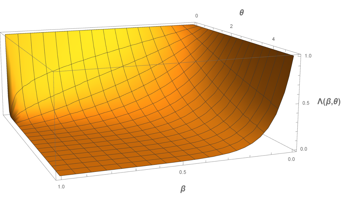
For each fixed $\beta\in(0,1)$, letting $\theta=0$ in Theorem 4 yields $\lim_{t\to\infty}F(x(t))/\bar{M}(t)=1$. The authors have previously obtained this conclusion for sublinear equations of the form (1.3) without regular variation but with $\lim_{t\to\infty}M(t)=M\in(0,\infty)$. Therefore Theorem 4 can be thought of as a continuous extension of our previous results for (1.1) with sublinear nonlinearities and finite measures (see [6] for further details).

For a fixed $\beta\in(0,1)$, a decrease in the value of $\theta$ represents an increase in the rate of decay of the measure $\mu$. This can be made precise by supposing that the measure $\mu$ is absolutely continuous, and specifically that $\mu(ds)=m(s)ds$ for continuous $m\in\text{RV}_{\infty}(\theta-1),\,\theta\in(0,1)$. Therefore, increasing the value of $\theta$ gives more weight to values of the solution in the past (more memory) and we expect the growth rate of solutions of (1.1) to be slower than that of the related ordinary differential equation

The equation (2.4), in contrast, places the entire weight $M(t)$ at the present time, when the solution is largest. Hence, increasing the value of $\theta$ (putting more weight further into the past) slows the growth rate and it is intuitive that $\Lambda(\beta,\theta)$ is decreasing in $\theta$. Using this comparison with (2.4) once more, it is clear that Proposition 1 $(v.)$ must hold since solutions of (1.1) can never grow faster than those of (2.4) (if $f$ is strictly increasing this can be seen by inspection).

For a fixed $\theta\in(0,\infty)$, one might expect an increase in $\beta$ to lead to a faster rate of growth of the solution of (1.1). Therefore, it may initially be surprising that $\Lambda(\beta,\theta)$ is decreasing in $\beta$. This counter-intuitive result is best understood by explaining the error introduced in the approximation of the right-hand side of (1.1). From (1.1)

The error of our upper bound on the solution is proportional to the ratio $f(x(t-s))/f(x(t))$ for $s\in(0,t)$, or $f(x(\lambda t))/f(x(t))$ for $\lambda\in(0,1)$. Since $f\circ x\in\text{RV}_{\infty}(\beta(1+\theta)/(1-\beta))$

When $\gamma(\beta)$ is close to one, the solution of (1.1) is close to that of (2.4) and hence our estimate is sharp. However, $\gamma(\beta)$ is decreasing and $\lim_{\beta\uparrow 1}\gamma(\beta)=0$. Thus the zero limit as $\beta\uparrow 1$ in Proposition 1 $(ii.)$ represents the fact that the solution of (2.4) increases much faster in $\beta$ than the solution to (1.1), for a fixed value of $\theta$.

We now present a result which illustrates how our precise understanding of the asymptotics of solutions of (1.1) can be applied to perturbed versions of the equation, such as (1.4). This result applies to perturbations of (1.1) that are of the same, or smaller, order of magnitude as solutions of the ordinary differential equation (2.4). Our assumptions on $H$ guarantee that $\lim_{t\to\infty}x(t)=\infty$ but this limit is no longer necessarily achieved monotonically and this is reflected in the added complexity of certain technical aspects of the proofs. The proofs of the results in this section are largely deferred to Section 5.

We notice that, when there is a sufficiently slowly growing forcing term $H$, $\lambda=0$, and we recover from (3.2) exactly the asymptotic behaviour of the unperturbed equation, given by (2.3). Also, in the limit as $\lambda\to 0^{+}$, the rate of the unperturbed equation is recovered.

Condition $(ii.)$ on $H$ in Theorem 5 does not cover the case when $H$ is of larger magnitude than the solution of the unperturbed equation (1.1) (or that of (2.4)). To deal with this case, we would like to know the growth rate of the solution when $\lim_{t\to\infty}H(t)/F^{-1}(t\,M(t))=\infty$. Insight into what happens can be gained by sending $\lambda\to\infty$ in Theorem 5. For $\lambda>0$, from Theorem 5, we have

where $\zeta$ depends on $\lambda$ through (3.2). Since $\zeta=\zeta(\lambda)$ is the unique positive solution of (3.2), $\eta=\eta(\lambda)$ is the unique positive solution of $\eta=1+K\eta^{\beta}\lambda^{\beta-1}$ where $K>0$ is the $\lambda$–independent positive quantity

Clearly $\eta(\lambda)>1$ and $\lambda\mapsto\eta(\lambda)$ is in $C^{1}$, by the implicit function theorem. Moreover, by implicit differentiation, $\eta^{\prime}(\lambda)$ obeys

Therefore, as the bracket on the left–hand side is positive, $\lambda\mapsto\eta(\lambda)$ is decreasing. Hence for $\lambda>1$, we have $\eta(\lambda)<1+K\eta(1)^{\beta}\lambda^{\beta-1}$, so $\limsup_{\lambda\to\infty}\eta(\lambda)\leq 1$, and so $\eta(\lambda)\to 1$ as $\lambda\to\infty$.

In view of this discussion, one might expect that $\lim_{t\to\infty}H(t)/F^{-1}(t\,M(t))=\infty$ implies $x(t)\sim H(t)$ as $t\to\infty$, or less precisely that sufficiently rapid growth in $H$ forces $x(t)$ to grow at the rate $H(t)$. Therefore, it is natural to ask under what conditions we would have $x(t)\sim H(t)$ as $t\to\infty$. It is straightforward to show that a necessary condition for $\lim_{t\to\infty}x(t)/H(t)=1$ is that $\lim_{t\to\infty}\int_{0}^{t}M(t-s)f(H(s))ds/H(t)=0$. This motivates the hypothesis

and the following result. This result requires no monotonicity in $H$ and as such allows for $H$ to undergo considerable fluctuation, a point we will illustrate further in Section 4.

When $H$ is regularly varying at infinity the hypotheses of Theorems 5 and 6 align to give a complete classification of the asymptotics (Corollary 1). However, assuming regular variation of $H$ imposes considerable regularity constraints. In particular, $H$ is then asymptotic to an increasing function and this restricts potential applications of Theorem 6 to stochastic functional differential equations.

We exclude the case $\alpha=0$, because it is covered by Theorem 5 with $\lambda=0$.

We state without proof a partial converse to Theorem 6 with $H\in\text{RV}_{\infty}(\alpha),\,\alpha>0$. The proof follows from Corollary 1 and estimation arguments similar to those used throughout this paper.

While discussing the hypothesis that $\lim_{t\to\infty}H(t)/F^{-1}(tM(t))=\infty$ in the context of regular variation it is worth remarking that this hypothesis is also satisfied for $H\in\text{RV}_{\infty}(\infty)$, the so-called rapidly varying functions (see [8, p.83]). If $H\in\text{RV}_{\infty}(\infty)$, then (3.3) holds and Theorem 6 can be applied; this fact is recorded in the following corollary.

Corollary 2 will also hold if $H\in\text{MR}_{\infty}(\infty)$, a sub-class of $\text{RV}_{\infty}(\infty)$ (see [8, p.68] for the definition of $\text{MR}_{\infty}(\infty)$), because this guarantees that $H$ is asymptotic to an increasing function (see [8, p.83]).

The requisite proofs and justifications supporting the discussion in this section are deferred to Section 6.

References

- [1] J. A. D. Appleby. On regularly varying and history-dependent convergence rates of solutions of a Volterra equation with infinite memory. Advances in Difference Equations, 2010(1):1–31, 2010.
- [2] J. A. D. Appleby and E. Buckwar. A constructive comparison technique for determining the asymptotic behaviour of linear functional differential equations with unbounded delay. Differential Equations and Dynamical Systems, 28(3):271–301, 2010.
- [3] J. A. D. Appleby, I. Győri, and D. W. Reynolds. On exact rates of decay of solutions of linear systems of Volterra equations with delay. J. Math. Anal. Appl, 320(1):56–77, 2006.
- [4] J. A. D. Appleby and K. Krol. Long memory in a linear stochastic volterra differential equation. J. Math. Anal. Appl., 380(2):814–830, 2011.
- [5] J. A. D. Appleby and D. D. Patterson. Classification of convergence rates of solutions of perturbed ordinary differential equations with regularly varying nonlinearity. arXiv preprint arXiv:1303.3345, to appear Electron. J. Qual. Theory Differ. Equ., Proc. 10th Coll. QTDE, Paper No. 2, pages 1–38, 2013.
- [6] J. A. D. Appleby and D. D. Patterson. Growth rates of sublinear functional and Volterra differential equations. arXiv preprint arXiv:1602.06256, pages 1–31, 2016.
- [7] J. A. D. Appleby and M. Riedle. Stochastic Volterra differential equations in weighted spaces. J. Integral Equ. Appl., 22(1):1–17, 2010.
- [8] N. H. Bingham, C. M. Goldie, and J. L. Teugels. Regular variation, volume 27. Cambridge University Press, 1989.
- [9] H. Brunner and S. Maset. Time transformations for delay differential equations. Discrete and Continuous Dynamical Systems, Series A, 25(3):751–775, 2009.
- [10] G. Gripenberg, S.-O. Londen, and O. Staffans. Volterra integral and functional equations, volume 34. Cambridge University Press, 1990.
- [11] K. B. Hannsgen. Indirect Abelian theorems and a linear Volterra equation. Trans. Amer. Math. Soc., 142:539–555, 1969.
- [12] V. Marić. Regular variation and differential equations, volume 1726. Springer, 2000.
- [13] F. Olver, D. Lozier, R. Boisvert, and C. Clark. NIST Handbook of Mathematical Functions, US Department of Commerce, National Institute of Standards and Technology, Washington, DC, 2010. Cambridge University Press, Cambridge, London and New York, 2010.
- [14] P. Řehák. Nonlinear differential equations in the framework of regular variation, 2014.
- [15] W. R. Schneider. The general solution of a non-linear integral equation of convolution type. Z. Angew. Math. Phys., 33(1):140–142, 1982.
- [16] D. F. Shea and S. Wainger. Variants of the Wiener-Lévy theorem, with applications to stability problems for some Volterra integral equations. American Journal of Mathematics, 97(2):312–343, 1975.
- [17] J. S. Wong and R. Wong. Asymptotic solutions of linear Volterra integral equations with singular kernels. Transactions of the American Mathematical Society, 189:185–200, 1974.