Leading QCD-induced four-loop contributions to the $\beta$-function of the Higgs self-coupling in the SM and vacuum stability

The evolution of the Higgs self-coupling and of the Higgs field are important ingredients for the Renormalization Group (RG) improved Higgs potential and the study of vacuum stability. A precise determination of the Higgs self-coupling in the Standard Model extended up to the Planck scale is important because this parameter is close to zero at the Planck scale and the question whether the SM vacuum state is stable or not can only be answered definitively by reducing the uncertainties.¹¹ 1 During the last years many detailed studies of the vacuum stability issue in the SM have been performed [4, 5, 6, 7, 8, 9, 10, 11, 12, 13, 14, 15, 16, 17] following the original ideas of [18, 19, 20]. A recent extension to the MSSM can be found in [21]. The largest source of uncertainty is the experimentally measured top mass $M_{\scriptscriptstyle{\text{t}}}$. At a future linear $e^{+}e^{-}$ collider it could, however, be measured with a precision which matches that of the theory input to the vacuum stability analysis (see Fig. 5 in [13]).

On the theory side there are three sources of uncertainty. The first is the difference between the effective Higgs potential $V_{\scriptscriptstyle{\text{eff}}}(\Phi_{\scriptscriptstyle{\text{cl}}})$ [22] and the approximation of the RG-improved potential

where $\Phi_{\scriptscriptstyle{\text{cl}}}=\langle 0|\Phi|0\rangle$ is the classical field strength of the scalar SU(2) doublet $\Phi$, $\gamma_{\scriptscriptstyle{\Phi}}$ the anomalous dimension of $\Phi$ and $\mu_{0}$ the scale where we start the evolution of fields and couplings, e. g. $\mu_{0}=M_{\scriptscriptstyle{\text{t}}}$. This uncertainty is negligible at large values of $\Phi_{\scriptscriptstyle{\text{cl}}}$, e. g. close to the Planck scale [23, 24, 25, 26, 27]. In this approximation the SM vacuum is stable up to the scale $\Lambda\sim M_{\scriptscriptstyle{\text{Planck}}}$ if $\lambda(\mu)>0$ for $\mu\leq\Lambda$.

Another source of theoretical uncertainties is the matching of experimental parameters, e. g. $M_{\scriptscriptstyle{\text{t}}},\alpha_{\scriptscriptstyle{s}}(M_{\scriptscriptstyle{\text{Z}}}),M_{\scriptscriptstyle{\text{H}}}$, to the parameters of the SM Lagrangian, $y_{\scriptscriptstyle{t}}(\mu_{0}),g_{\scriptscriptstyle{s}}(\mu_{0}),\lambda(\mu_{0}),\ldots$ at some initial scale $\mu_{0}$ renormalized in the $\overline{\text{MS}}$-scheme. State of the art is the full numerical two-loop matching [16, 28]. In order to improve precision here three-loop calculations might be attempted and different mass definitions than the pole mass could be used for the top mass.

In this paper we improve on the third source of uncertainty, namely we increase the precision in the $\beta$-functions, calculated in the $\overline{\text{MS}}$-scheme. The $\beta$-function for a coupling $X$ is defined as

and the anomalous dimension of a field $f$ as

where $Z_{\scriptscriptstyle{f}}$ is the field strength renormalization constant, where $X,X_{1},X_{2},\ldots$ are the couplings of the theory which we want to include in the analysis.

The RG functions of the SM were computed at three-loop accuracy during the last years [29, 30, 31, 10, 32, 33, 34, 35]. The four-loop $\beta$-function for the strong coupling $g_{\scriptscriptstyle{s}}$ was first computed in pure QCD [36, 37] and recently extended to the gaugeless limit of the SM, namely to include the dependence on the top-Yukawa coupling $y_{\scriptscriptstyle{t}}$ and the Higgs self-coupling $\lambda$ [2, 3]. The leading four-loop contribution to the Higgs self-coupling $\beta$-function was first presented in [1] and is independently confirmed in this paper.

The paper is structured as follows: In the next section we briefly describe the technical details of the calculation. Then the leading four-loop terms for $\beta_{\lambda}$, $\beta_{y_{\scriptscriptstyle{t}}}$ and $\gamma_{2}^{\scriptscriptstyle{\Phi}}$ are given and the relevance of the four-loop terms numerically determined at the scale of the top quark mass. Finally, we investigate the impact of the new contributions on the evolution of $\lambda$ in order to estimate the uncertainty reduction due to four-loop $\beta$-functions.

In this section we give our results which can be found in machine readable format on
http://www-ttp.particle.uni-karlsruhe.de/Progdata/ttp16/ttp16-008/
For a gerneric SU($N_{\scriptscriptstyle{c}}$) gauge group the colour factors are expressed through the quadratic Casimir operators $C_{\scriptscriptstyle{F}}$ and $C_{\scriptscriptstyle{A}}$ of the fundamental and the adjoint representation of the corresponding Lie algebra. The dimension of the fundamental representation is called $d_{\scriptscriptstyle{R}}$. The adjoint representation has dimension $n_{\scriptscriptstyle{g}}$ and the trace $T_{\scriptscriptstyle{F}}$ is defined by $T_{\scriptscriptstyle{F}}\delta^{ab}=\textbf{Tr}\left(T^{a}T^{b}\right)$ with the group generators $T^{a}$ of the fundamental representation. Higher order invariants are constructed from the symmetric tensors

from the generators of the fundamental representation and analogously $d_{\scriptscriptstyle{A}}^{abcd}$ from the generators of the adjoint representation. The combinations needed and their SU($N_{\scriptscriptstyle{c}}$) values are

Furthermore for SU($N_{\scriptscriptstyle{c}}$) we have

The number of active fermion flavours is denoted by $n_{\scriptscriptstyle{f}}$. The leading four-loop contributions to the $\beta$-functions for the Higgs self-coupling and the top-Yukawa coupling are found to be

in agreement³³ 3 Note that in [1] the definition $\beta_{\lambda}^{\scriptscriptstyle{\text{S.M.}}}=\mu\frac{d\lambda}{d\mu}=2\beta_{\lambda}$ for the $\beta$-function is used. with eq. (4.32) of [1] and

The leading contribution to the anomalous dimension of the Higgs field (or equivalently the scalar SU(2) doublet $\Phi$) at four-loop level is given by

For the lower loop contributions we refer to [10, 32, 33, 34, 35].

All diagrams discussed in the previous section are special in one aspect: they comprise just the minimal number of non-QCD vertexes, that is one for $\beta_{y_{t}}$, two for $\gamma_{2}^{\Phi}$ and four for $\beta_{\lambda}$. Even more, these non-QCD vertexes are of one and the same type, namely the insertion of the scalar top-quark current $\bar{t}\,t$. This means that the corresponding anomalous dimensions should be related to some RG functions in pure QCD describing the QCD evolution of the scalar current(s). The corresponding “effective” Lagrangian

implies, obviously, the following identities valid in all orders in $\alpha_{s}$ (dots below stand for terms which have a different dependence on the SM coupling constants than $y_{t}\,\alpha_{s}^{n}$ (first line) and $y^{2}_{t}\,\alpha_{s}^{n}$ (second line) correspondingly):

Here $\gamma_{m}(\alpha_{s})$ is the quark mass anomalous dimension and the function $\gamma^{SS}_{q}(\alpha_{s})$ appears in the evolution equation

for the scalar correlator ($B$ marking bare quantities)

which is renormalized as

The anomalous dimensions are found to be

Needless to say that a comparison with available results for $\gamma_{m}(\alpha_{s})$ [49, 50] and $\gamma^{SS}_{q}(\alpha_{s})$ [51] confirms the relations (15) and (16) at four-loop order⁴⁴ 4 In fact, both quantities are currently also known to five loops from [52, 53]. .

Finally, let us consider in some detail the last (and somewhat more complicated) case, viz. the $\beta$-function for the Higgs self-coupling $\beta_{\lambda}$. The corresponding renormalization constant coincides up to a factor $\frac{y_{t}^{4}}{4\cdot 4!}$ to that which renormalizes the (1PI) Green’s function of the T-product of four scalar currents:

With $m_{t}\not=0$ we could nullify all external momenta $p_{i}$ in eq. (22) and, thus, consider all $j_{s}$-operators on the rhs of (22) as insertions of the scalar quark current at zero momentum transfer.

As is well-known such insertions can be generated by multiple differentiations of QCD Green functions wrt a quark mass⁵⁵ 5 For the Higgs decay via heavy top loops such relations have been known as low-energy theorems for a long time [54, 55, 56, 57].. This means that the corresponding anomalous dimensions should be related to some pure QCD RG functions. The well-known way to construct the corresponding relations is to use the (renormalized) Quantum Action Principle [58, 59]. Let us briefly outline the main points.

The Quantum Action Principle relates properties of (regularized) Lagrangian and the full Green’s functions. Consider the generating functional of (connected) Green’s functions

defined in

The Action Principle states (in particular) that

where $\lambda$ is a any parameter in the Lagrangian ${\cal L}$. The action principle works for DR Green functions [60] (modulo axial anomalies).

An example: the (renormalized) QCD Lagrangian with $n_{l}$ massless quarks and a massive (top) one is customarily written as

With properly chosen renormalization constants $Z_{i}$ (26) should produce finite Green’s functions. If one differentiates $W(J)$ wrt the (renormalized) top quark mass $m_{t}$ the functional

should also be finite. However, let us consdider eq. (27) at $J=0$. It corresponds, obviously, to the VEV of the operator $Z_{m}Z_{2}\,\bar{t}t(x)$, which is not finite already at order $\alpha_{s}^{0}$ (a couple of typical diagrams contributing to (27) at $J=0$ are shown on Fig. 4).

This means that our QCD Lagrangian (26) is not full: the term responsible for the renormalization of the vacuum energy is missing. The full QCD Lagrangian reads [61]

here $E_{0}(\mu)$ is the (renormalized) vacuum energy and $Z_{0}$ is the corresponding renormalization constant.

Now, a four-fold differentiation of the generating functional (24) (with $\mathcal{L}=\mathcal{L}_{QCD}^{{\scriptscriptstyle{full}}}$) wrt $m_{t}$ immediately leads us to the conclusion that the combination

should be finite. As a result, we arrive at the following identity valid in all orders in $\alpha_{s}$:

where the dots stand for terms which have a different dependence on the SM coupling constants than $y^{4}_{t}\,\alpha_{s}^{n}$ and⁶⁶ 6 We define the QCD $\beta$-function as $\normalsize\beta(\alpha_{\scriptscriptstyle{s}})=\frac{d\alpha_{\scriptscriptstyle{s}}}{d\ln\mu^{2}}$.

is the anomalous dimension of the vaccuum energy

The vacuum anomalous dimension plays an important role in the description of the renormalization mixing of all three scalar gauge-invariant operators with (mass) dimension four:

It was proven in [62, 61] that the matrix of anomalous dimensions in (34) reads:

In addition, the two-point scalar correlator (16) at $q=0$ is obviously related (via the Action Principle) to the four-point correlator (22), as the latter can be obtained from the former by a double differentiation wrt $m_{t}$. This, in turn, leads to the following remarkable relation (again valid in all orders in $\alpha_{s}$):

Thus, one could compute $\gamma_{0}$ in a few different ways.

1. Direct renormalization of the vacuum energy diagrams. This was done for two and three loops in the papers [61] and [63] respectively. At four loops it was first found in this way for a space-time dimension $D=3$ [64, 65] (in the process of computing the free energy in the effective high temperature QCD) and (implicitly, via eq. (30)) in the present paper.

2. By renormalizing the 4-loop scalar correlator [66] in the limit of small quark mass⁷⁷ 7 That is the scalar corelator was expanded at the large momentum limit and the $\gamma_{m}^{SS}$ was found by renormalizing the term of order $m_{t}^{2}/Q^{2}$.. The result was later used in [67] to compute the quartic mass corrections to $R_{had}$ at ${\cal O}(\alpha_{s}^{3})$.

3. By computing the lowest moment of the scalar correlator at 4 loops [68].

4. By computing the lowest low-energy moment of the axial-vector correlator (related via a Ward identity to the VEV of the scalar current) [69].

Note, finally, that the last two evaluations dealt with massive tadpole diagrams and that all calculations of $\gamma_{0}$ at the four-loop level described above are in mutual agreement as well as the two results for $\beta_{\lambda}^{(4)}$: the one displayed in (11) and the one obtained via relation (30).

In this section we want to numerically evaluate the results for the $\beta$-functions presented in section 3. The couplings $g_{\scriptscriptstyle{s}},g_{2},g_{1},y_{\scriptscriptstyle{t}}$ and $\lambda$ in the $\overline{\text{MS}}$-scheme at some fixed scale $\mu_{0}$ can be computed by matching the experimentally measured parameters $\alpha_{\scriptscriptstyle{s}}(M_{\scriptscriptstyle{\text{Z}}})$, $G_{F}$, $M_{W}$, $M_{Z}$, $M_{\scriptscriptstyle{\text{t}}}$ and $M_{\scriptscriptstyle{\text{H}}}$ to them [16, 28], where the uncertainties of $G_{F}$, $M_{W}$ and $M_{Z}$ have a negligible influence on the $\overline{\text{MS}}$-couplings as compared to the other three. The Higgs mass is taken to be $M_{\scriptscriptstyle{\text{H}}}=125.09\pm 0.24$ GeV [70] and the strong coupling is extracted from $\alpha_{\scriptscriptstyle{s}}(M_{\scriptscriptstyle{\text{Z}}})=0.1181\pm 0.0013$ [71].

The top mass is a more difficult subject. At the moment a theoretically well-defined mass is not available to high prescision. The extraction of an $\overline{\text{MS}}$-mass from cross section measurements leads to an uncertainty of $4-5$ GeV [71], the extraction of the pole mass from cross section measurements to [71]

The most precise top mass measurements from LHC and TEVATRON give $M_{\scriptscriptstyle{\text{t}}}^{\scriptscriptstyle{\text{MC}}}\approx 173.34\pm 0.76$ GeV [72] where the Monte Carlo mass parameter $M_{\scriptscriptstyle{\text{t}}}^{\scriptscriptstyle{\text{MC}}}$ would correspond to the pole mass in a purely perturbative setup. Since $M_{\scriptscriptstyle{\text{t}}}^{\scriptscriptstyle{\text{MC}}}$ is affected by real emission and the implementation of the parton shower it eludes a theoretical definition based on the Lagrangian but has to be calibrated to fit the experimental data. The pole mass of a heavy quark also suffers from a conceptual problem, namely the renormalon ambiguity [73, 74]. This is due to the fact that a quark is not observed as a free particle and non-perturbative effects spoil the convergence of the relations between the pole mass and e. g. an $\overline{\text{MS}}$-mass. One way to connect the Monte Carlo and the pole mass is to identify the first with a theoretically well-defined short-distance mass at a scale $R\sim 1-3$ GeV, i. e. the parton shower cut-off of the Monte Carlo simulation [75]. This so-called MSR mass does not suffer from non-perturbative effects such as renormalons due to the IR cutoff. The MSR mass can in turn be connected to the pole mass (by adding the contributions from the IR region) [76] leading to $M_{\scriptscriptstyle{\text{t}}}^{\scriptscriptstyle{\text{pole}}}=173.39\pm 0.76\text{(exp)}{}^{+0.82}_{-0.62}\text{(th)}$ GeV for $M_{\scriptscriptstyle{\text{t}}}^{\scriptscriptstyle{\text{MC}}}=M_{\scriptscriptstyle{\text{t}}}^{\scriptscriptstyle{\text{MSR}}}(3^{+6}_{-2})\text{GeV}$ [77] or combining these errors in quadrature

For the following analysis we take this value which is very close to the Monte Carlo mass, noting however that the discrepancy with the current PDG top pole mass value (37) indicates that the uncertainties on this parameter might be even larger and a direct and precise extraction of theoretically well-defined quantities like the MSR mass or the $\overline{\text{MS}}$ top-Yukawa coupling itself from the experimental data of a linear collider will be necessary in order to match the size of the other uncertainties entering the vacuum stability analysis.

For $M_{\scriptscriptstyle{\text{t}}}=173.39{}^{+1.12}_{-0.98}$ GeV [72, 77] we get the couplings in the $\overline{\text{MS}}$-scheme at the scale of the top mass using two-loop matching relations [16]

where the experimental uncertainty (exp) stems from $M_{t},M_{H}$ and $\alpha_{\scriptscriptstyle{s}}(M_{Z})$ and the theoretical one (theo) from the matching of on-shell to $\overline{\text{MS}}$ parameters [16]. Evaluating $\beta_{\scriptscriptstyle{y_{\scriptscriptstyle{t}}}}$ at the scale $M_{\scriptscriptstyle{\text{t}}}$ we find

which shows the expected suppression of higher order contributions. The four-loop terms are significantly smaller than the lower loop terms. For $\beta_{\scriptscriptstyle{\lambda}}$ however the picture is different. Already in previous works [10, 32, 78] we found a slow convergence of the perturbation series up to three-loop order at the electroweak scale and this is also found true at four-loop level:

As discussed in [32, 78] there is a remarkable cancellation between the terms containing only $g_{\scriptscriptstyle{s}}$ and $y_{\scriptscriptstyle{t}}$ at two-loop⁸⁸ 8 Here for example the numerically largest terms $\propto y_{\scriptscriptstyle{t}}^{4}g_{\scriptscriptstyle{s}}^{2}$, $\propto y_{\scriptscriptstyle{t}}^{6}$ and $\propto\lambda y_{\scriptscriptstyle{t}}^{2}g_{\scriptscriptstyle{s}}^{2}$ cancel so well that the sum of these terms is only about $2-3\%$ of the size of the largest term $\propto y_{\scriptscriptstyle{t}}^{4}g_{\scriptscriptstyle{s}}^{2}$ at $\mu=M_{\scriptscriptstyle{\text{t}}}$. and three-loop level at the scale of the top mass making the overall contribution much smaller than the size of the individual terms. These cancellations seem to accidental, so we cannot predict there existence at four-loop level. However, if the cancellation also exists at this order the terms $\propto y_{\scriptscriptstyle{t}}^{6}g_{\scriptscriptstyle{s}}^{4},\,\propto y_{\scriptscriptstyle{t}}^{8}g_{\scriptscriptstyle{s}}^{2},\,\propto y_{\scriptscriptstyle{t}}^{10},$ etc could make the result significantly smaller and hence increase the convergence of the perturbative series. At higher scales, where $g_{\scriptscriptstyle{s}}$ and $y_{\scriptscriptstyle{t}}$ become smaller the convergence is of course better also if we only include the term $\propto y_{\scriptscriptstyle{t}}^{4}g_{\scriptscriptstyle{s}}^{6}$. At $\mu=10^{9}\text{GeV}$ we find

where the leading four-loop contribution is a factor $4-5$ smaller than the three-loop result but still not completely negligible. We will now check what this means for the evolution of the Higgs self-coupling $\lambda$ up to the Planck scale.

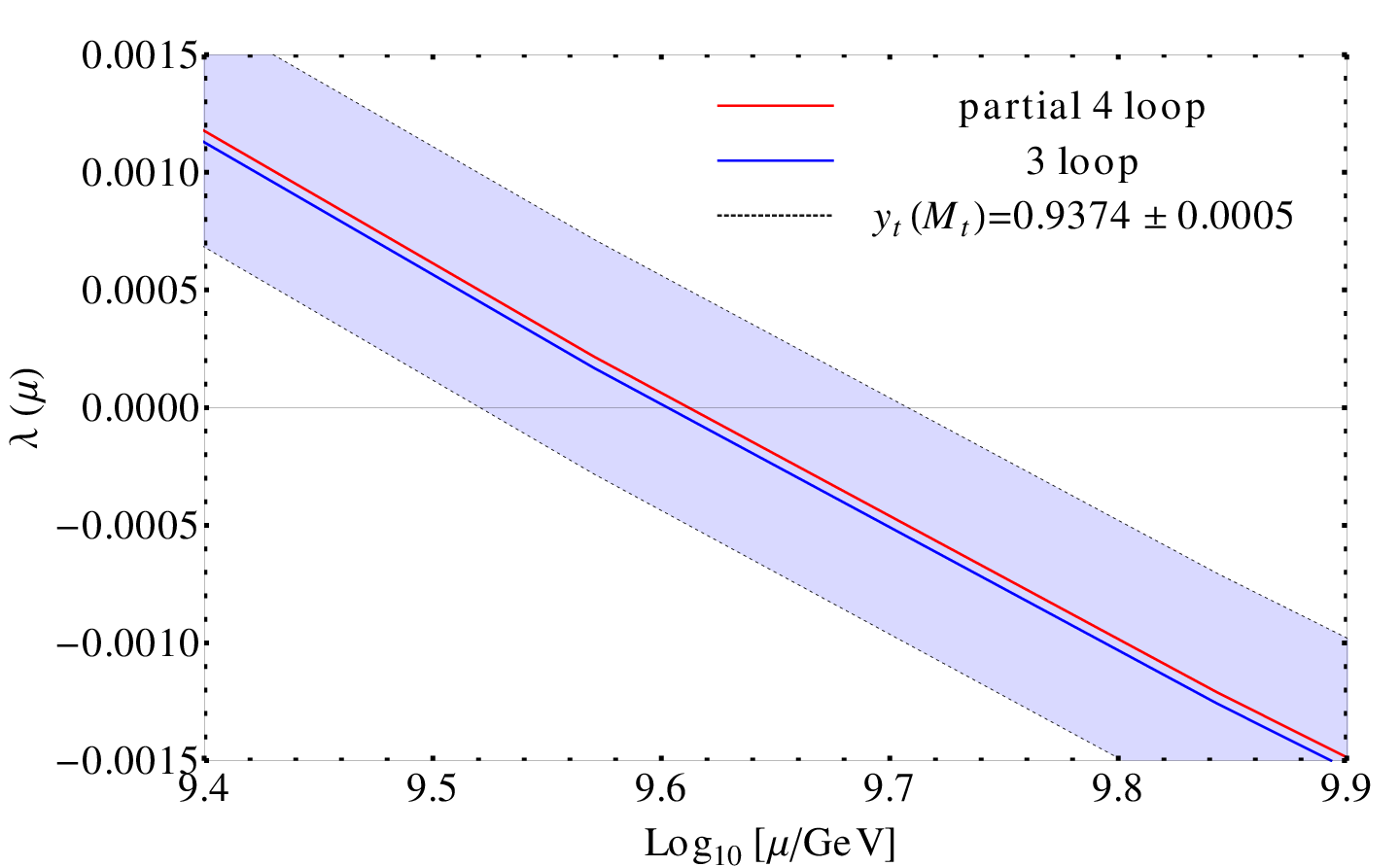
We evolve $\lambda$ from the scale $M_{\scriptscriptstyle{\text{t}}}$ using the initial conditions (39) and the full SM $\beta$-functions (including $g_{\scriptscriptstyle{s}},y_{\scriptscriptstyle{t}},g_{2},g_{1},\lambda$) up to three-loop order and at four-loop level $\beta^{(4)}_{g_{\scriptscriptstyle{s}}}(g_{\scriptscriptstyle{s}},y_{\scriptscriptstyle{t}},\lambda)$ [2, 3] and the leading contributions to $\beta^{(4)}_{y_{\scriptscriptstyle{t}}}(g_{\scriptscriptstyle{s}},y_{\scriptscriptstyle{t}})$ and $\beta^{(4)}_{\lambda}(g_{\scriptscriptstyle{s}},y_{\scriptscriptstyle{t}})$, as given in (12) and (11). Fig. 5 shows the result compared to the largest remaining uncertainties on the theory and on the experimental side. The smaller error band marks the $1\sigma$ uncertainty stemming from the top matching, i.e. we vary $y_{\scriptscriptstyle{t}}$ by $\pm 0.0005$ (see (39)). The larger error band marks the $1\sigma$ uncertainty stemming from the top pole mass.

The difference between the evolution of $\lambda$ with three-loop $\beta$-functions (blue curve) and including the leading four-loop terms (red curve) should give some indication on the uncertainty stemming from the truncation of the perturbative series for the $\beta$-functions. In order to see this difference we have to zoom in. We choose to do this at the scale where $\lambda$ becomes negative, which is shown in Fig. 6. The error bands are calculated using the partial four-loop results and hence centered around the red curve.

In order to further illustrate the dependence of the vacuum stability problem on the top mass and the importance of the issues related to the top pole mass as an input parameter we show the evolution of $\lambda$ also for the PDG value extracted from cross section measurements of the top pole mass (37) and the corresponding uncertainties in Fig. 7.

The conclusion for vacuum stability remains the same as in our previous works [10, 11, 13, 14, 15]. It looks as if $\lambda$ becomes negative at around $\log_{10}\left(\frac{\mu}{\text{GeV}}\right)\sim 9.6$ (or $\log_{10}\left(\frac{\mu}{\text{GeV}}\right)\sim 8.7$ in Fig. 7) rendering the SM not stable if extended up to scales above, but a definitive answer is pending on a more precise extraction of $y_{\scriptscriptstyle{t}}(\mu_{0})$ from experimental data. It is worth noting, however, that due to the reduction in the top mass uncertainty since the combined LHC and TEVATRON analysis [72] a stable SM up to the Planck scale is strongly disfavoured.

In this work we have presented analytical results for the leading four-loop contributions to the $\beta$-function for the Higgs self-coupling $\lambda$ and the top-Yukawa coupling as well as to the anomalous dimension of the Higgs field. These results have been connected to pure QCD RG functions and a relation between the anmalous dimension $\gamma_{0}$ of the vacuum energy and $\gamma^{SS}_{m}$ was found. We have performed an analysis of the evolution of the Higgs self-coupling updating the analyses presented in previous works [10, 11, 13, 14, 15] and establishing a nice hirarchy between the different sources of uncertainty.

With the computation of the leading four-loop terms to $\beta_{\lambda},\beta_{y_{\scriptscriptstyle{t}}}$ and $\beta_{g_{\scriptscriptstyle{s}}}$ the $\beta$-function uncertainty to the question of vacuum stability becomes significantly smaller than the matching uncertainty (before the two were comparable) which is in turn significantly smaller than the experimental top mass uncertainty. We expect that a full calculation of four-loop $\beta$-functions in the SM will confirm this conclusion rendering the remaining $\beta$-function uncertainty almost negligible in comparison to the other sources of uncertainty for a vacuum stability analysis.

One of us (K. Ch.) thanks Mikhail Shaposhnikov for a hint about a possible connection between the vacuum energy and $\beta_{\lambda}$.

This research was supported in part by the Swiss National Science Foundation (SNF) under contract BSCGI0_157722. The work by K. Ch. was supported by the Deutsche Forschungsgemeinschaft through CH1479/1-1.

References

- (1) S. P. Martin, Four-loop Standard Model effective potential at leading order in QCD, Phys. Rev. D92 (2015) 054029, [1508.00912].
- (2) A. V. Bednyakov and A. F. Pikelner, Four-loop strong coupling beta-function in the Standard Model, 1508.02680.
- (3) M. F. Zoller, Top-Yukawa effects on the -function of the strong coupling in the SM at four-loop level, JHEP 02 (2016) 095, [1508.03624].
- (4) F. Bezrukov and M. Shaposhnikov, Standard Model Higgs boson mass from inflation: two loop analysis, JHEP 07 (2009) 089, [0904.1537].
- (5) M. Holthausen, K. S. Lim and M. Lindner, Planck scale Boundary Conditions and the Higgs Mass, JHEP 1202 (2012) 037, [1112.2415].
- (6) J. Elias-Miro, J. R. Espinosa, G. F. Giudice, G. Isidori, A. Riotto et al., Higgs mass implications on the stability of the electroweak vacuum, Phys. Lett. B709 (2012) 222–228, [1112.3022].
- (7) Z.-z. Xing, H. Zhang and S. Zhou, Impacts of the Higgs mass on vacuum stability, running fermion masses and two-body Higgs decays, Phys. Rev. D86 (2012) 013013, [1112.3112].
- (8) F. Bezrukov, M. Y. Kalmykov, B. A. Kniehl and M. Shaposhnikov, Higgs Boson Mass and New Physics, JHEP 1210 (2012) 140, [1205.2893].
- (9) G. Degrassi, S. Di Vita, J. Elias-Miro, J. R. Espinosa, G. F. Giudice et al., Higgs mass and vacuum stability in the Standard Model at NNLO, JHEP 1208 (2012) 098, [1205.6497].
- (10) K. Chetyrkin and M. Zoller, Three-loop -functions for top-Yukawa and the Higgs self-interaction in the Standard Model, JHEP 1206 (2012) 033, [1205.2892].
- (11) M. F. Zoller, Vacuum stability in the SM and the three-loop -function for the Higgs self-interaction, Subnucl. Ser. 50 (2014) 557–566, [1209.5609].
- (12) I. Masina, Higgs boson and top quark masses as tests of electroweak vacuum stability, Phys.Rev. D87 (2013) 053001, [1209.0393].
- (13) M. F. Zoller, Standard Model beta-functions to three-loop order and vacuum stability, in 17th International Moscow School of Physics and 42nd ITEP Winter School of Physics Moscow, Russia, February 11-18, 2014, 2014. 1411.2843.
- (14) M. Zoller, Three-loop beta function for the Higgs self-coupling, PoS LL2014 (2014) 014, [1407.6608].
- (15) M. Zoller, Beta-function for the Higgs self-interaction in the Standard Model at three-loop level, PoS (EPS-HEP 2013) (2013) 322, [1311.5085].
- (16) D. Buttazzo, G. Degrassi, P. P. Giardino, G. F. Giudice, F. Sala, A. Salvio et al., Investigating the near-criticality of the Higgs boson, JHEP 12 (2013) 089, [1307.3536].
- (17) A. V. Bednyakov, B. A. Kniehl, A. F. Pikelner and O. L. Veretin, Stability of the Electroweak Vacuum: Gauge Independence and Advanced Precision, Phys. Rev. Lett. 115 (2015) 201802, [1507.08833].
- (18) N. V. Krasnikov, Restriction of the Fermion Mass in Gauge Theories of Weak and Electromagnetic Interactions, Yad. Fiz. 28 (1978) 549–551.
- (19) H. D. Politzer and S. Wolfram, Bounds on Particle Masses in the Weinberg-Salam Model, Phys. Lett. B82 (1979) 242–246.
- (20) P. Q. Hung, Vacuum Instability and New Constraints on Fermion Masses, Phys. Rev. Lett. 42 (1979) 873.
- (21) M. Bobrowski, G. Chalons, W. G. Hollik and U. Nierste, Vacuum stability of the effective Higgs potential in the Minimal Supersymmetric Standard Model, Phys.Rev. D90 (2014) 035025, [1407.2814].
- (22) S. Coleman and E. Weinberg, Radiative corrections as the origin of spontaneous symmetry breaking, Phys. Rev. D 7 (1973) 1888–1910.
- (23) N. Cabibbo, L. Maiani, G. Parisi and R. Petronzio, Bounds on the Fermions and Higgs Boson Masses in Grand Unified Theories, Nucl. Phys. B158 (1979) 295–305.
- (24) M. Sher, Electroweak Higgs Potentials and Vacuum Stability, Phys.Rept. 179 (1989) 273–418.
- (25) M. Lindner, M. Sher and H. W. Zaglauer, Probing Vacuum Stability Bounds at the Fermilab Collider, Phys.Lett. B228 (1989) 139.
- (26) C. Ford, D. Jones, P. Stephenson and M. Einhorn, The Effective potential and the renormalization group, Nucl. Phys. B395 (1993) 17–34, [hep-lat/9210033].
- (27) G. Altarelli and G. Isidori, Lower limit on the higgs mass in the standard model: An update, Physics Letters B 337 (1994) 141–144.
- (28) B. A. Kniehl, A. F. Pikelner and O. L. Veretin, Two-loop electroweak threshold corrections in the Standard Model, Nucl. Phys. B896 (2015) 19–51, [1503.02138].
- (29) L. N. Mihaila, J. Salomon and M. Steinhauser, Gauge coupling beta functions in the standard model to three loops, Phys. Rev. Lett. 108 (2012) 151602.
- (30) L. N. Mihaila, J. Salomon and M. Steinhauser, Renormalization constants and beta functions for the gauge couplings of the Standard Model to three-loop order, Phys. Rev. D 86 (2012) 096008, [1208.3357].
- (31) A. Bednyakov, A. Pikelner and V. Velizhanin, Anomalous dimensions of gauge fields and gauge coupling beta-functions in the Standard Model at three loops, JHEP 1301 (2013) 017, [1210.6873].
- (32) K. G. Chetyrkin and M. F. Zoller, -function for the Higgs self-interaction in the Standard Model at three-loop level, JHEP 04 (2013) 091, [1303.2890].
- (33) A. Bednyakov, A. Pikelner and V. Velizhanin, Yukawa coupling beta-functions in the Standard Model at three loops, Phys.Lett. B722 (2013) 336–340, [1212.6829].
- (34) A. Bednyakov, A. Pikelner and V. Velizhanin, Higgs self-coupling beta-function in the Standard Model at three loops, Nucl.Phys. B875 (2013) 552–565, [1303.4364].
- (35) A. V. Bednyakov, A. F. Pikelner and V. N. Velizhanin, Three-loop Higgs self-coupling beta-function in the Standard Model with complex Yukawa matrices, Nucl. Phys. B879 (2014) 256–267, [1310.3806].
- (36) T. van Ritbergen, J. Vermaseren and S. Larin, The Four loop beta function in quantum chromodynamics, Phys. Lett. B400 (1997) 379–384, [hep-ph/9701390].
- (37) M. Czakon, The Four-loop QCD beta-function and anomalous dimensions, Nucl.Phys. B710 (2005) 485–498, [hep-ph/0411261].
- (38) P. Nogueira, Automatic Feynman graph generation, J. Comput. Phys. 105 (1993) 279–289.
- (39) T. Seidensticker, Automatic application of successive asymptotic expansions of Feynman diagrams, in 6th International Workshop on New Computing Techniques in Physics Research: Software Engineering, Artificial Intelligence Neural Nets, Genetic Algorithms, Symbolic Algebra, Automatic Calculation (AIHENP 99) Heraklion, Crete, Greece, April 12-16, 1999, 1999. hep-ph/9905298.
- (40) R. Harlander, T. Seidensticker and M. Steinhauser, Complete corrections of Order alpha alpha-s to the decay of the Z boson into bottom quarks, Phys.Lett. B426 (1998) 125–132, [hep-ph/9712228].
- (41) J. A. M. Vermaseren, New features of FORM, math-ph/0010025.
- (42) M. Tentyukov and J. A. M. Vermaseren, The Multithreaded version of FORM, Comput. Phys. Commun. 181 (2010) 1419–1427, [hep-ph/0702279].
- (43) T. Van Ritbergen, A. Schellekens and J. Vermaseren, Group theory factors for feynman diagrams, International Journal of Modern Physics A 14 (1999) 41–96.
- (44) M. Misiak and M. Münz, Two loop mixing of dimension five flavor changing operators, Phys. Lett. B344 (1995) 308–318, [hep-ph/9409454].
- (45) K. G. Chetyrkin, M. Misiak and M. Münz, Beta functions and anomalous dimensions up to three loops, Nucl. Phys. B518 (1998) 473–494, [hep-ph/9711266].
- (46) M. Steinhauser, MATAD: A program package for the computation of massive tadpoles, Comput. Phys. Commun. 134 (2001) 335–364, [hep-ph/0009029].
- (47) A. Smirnov, Algorithm FIRE – Feynman Integral REduction, JHEP 0810 (2008) 107, [0807.3243].
- (48) A. V. Smirnov, FIRE5: a C++ implementation of Feynman Integral REduction, Comput.Phys.Commun. 189 (2014) 182–191, [1408.2372].
- (49) J. A. M. Vermaseren, S. A. Larin and T. van Ritbergen, The 4-loop quark mass anomalous dimension and the invariant quark mass, Phys. Lett. B405 (1997) 327–333, [hep-ph/9703284].
- (50) K. G. Chetyrkin, Quark mass anomalous dimension to , Phys. Lett. B404 (1997) 161–165, [hep-ph/9703278].
- (51) K. G. Chetyrkin, Correlator of the quark scalar currents and at in pQCD, Phys. Lett. B390 (1997) 309–317, [hep-ph/9608318].
- (52) P. A. Baikov, K. G. Chetyrkin and J. H. Kühn, Quark Mass and Field Anomalous Dimensions to , JHEP 10 (2014) 076, [1402.6611].
- (53) P. A. Baikov, K. G. Chetyrkin and J. H. Kühn, Scalar correlator at Higgs decay into b-quarks and bounds on the light quark masses, Phys. Rev. Lett. 96 (2006) 012003, [hep-ph/0511063].
- (54) J. R. Ellis, M. K. Gaillard and D. V. Nanopoulos, A Phenomenological Profile of the Higgs Boson, Nucl. Phys. B106 (1976) 292.
- (55) M. A. Shifman, A. I. Vainshtein and V. I. Zakharov, Remarks on Higgs Boson Interactions with Nucleons, Phys. Lett. B78 (1978) 443.
- (56) B. A. Kniehl and M. Spira, Low-energy theorems in Higgs physics, Z. Phys. C69 (1995) 77–88, [hep-ph/9505225].
- (57) K. G. Chetyrkin, B. A. Kniehl and M. Steinhauser, Decoupling relations to and their connection to low-energy theorems, Nucl. Phys. B510 (1998) 61–87, [hep-ph/9708255].
- (58) J. H. Lowenstein, Differential vertex operations in Lagrangian field theory, Commun. Math. Phys. 24 (1971) 1–21.
- (59) Y.-M. P. Lam, Perturbation Lagrangian theory for scalar fields: Ward-Takahasi identity and current algebra, Phys. Rev. D6 (1972) 2145–2161.
- (60) P. Breitenlohner and D. Maison, Dimensional Renormalization and the Action Principle, Commun. Math. Phys. 52 (1977) 11–38.
- (61) V. P. Spiridonov and K. G. Chetyrkin, Nonleading mass corrections and renormalization of the operators and , Sov. J. Nucl. Phys. 47 (1988) 522–527.
- (62) V. P. Spiridonov, Anomalous Dimension of and Function, preprint IYaI-P-0378 (1984) .
- (63) K. G. Chetyrkin and J. H. Kühn, Quartic mass corrections to R(had), Nucl. Phys. B432 (1994) 337–350, [hep-ph/9406299].
- (64) Y. Schroder, Automatic reduction of four loop bubbles, Nucl.Phys.Proc.Suppl. 116 (2003) 402–406, [hep-ph/0211288].
- (65) F. Di Renzo, A. Mantovi, V. Miccio and Y. Schroder, 3-d lattice qcd free energy to four loops, JHEP 05 (2004) 006, [hep-lat/0404003].
- (66) K. G. Chetyrkin, 1998, unpublished .
- (67) K. G. Chetyrkin, R. V. Harlander and J. H. Kühn, Quartic mass corrections to at , Nucl. Phys. B586 (2000) 56–72, [hep-ph/0005139].
- (68) C. Sturm, Moments of Heavy Quark Current Correlators at Four-Loop Order in Perturbative QCD, JHEP 09 (2008) 075, [0805.3358].
- (69) A. Maier, P. Maierhofer, P. Marquard and A. V. Smirnov, Low energy moments of heavy quark current correlators at four loops, Nucl. Phys. B824 (2010) 1–18, [0907.2117].
- (70) ATLAS, CMS collaboration, G. Aad et al., Combined Measurement of the Higgs Boson Mass in Collisions at and 8 TeV with the ATLAS and CMS Experiments, Phys. Rev. Lett. 114 (2015) 191803, [1503.07589].
- (71) Particle Data Group collaboration, K. Olive et al., Review of Particle Physics, Chin.Phys. C38 (2014) 090001 and 2015 update.
- (72) ATLAS, CDF, CMS and D0, First combination of Tevatron and LHC measurements of the top-quark mass, 1403.4427.
- (73) I. I. Bigi, M. A. Shifman, N. Uraltsev and A. Vainshtein, The Pole mass of the heavy quark. Perturbation theory and beyond, Phys.Rev. D50 (1994) 2234–2246, [hep-ph/9402360].
- (74) M. Beneke, Renormalons, Phys.Rept. 317 (1999) 1–142, [hep-ph/9807443].
- (75) A. H. Hoang, A. Jain, I. Scimemi and I. W. Stewart, Infrared Renormalization Group Flow for Heavy Quark Masses, Phys. Rev. Lett. 101 (2008) 151602, [0803.4214].
- (76) S. Moch et al., High precision fundamental constants at the TeV scale, 1405.4781.
- (77) S. Moch, Precision determination of the top-quark mass, PoS LL2014 (2014) 054, [1408.6080].
- (78) K. G. Chetyrkin and M. F. Zoller, Erratum: -function for the Higgs self-interaction in the Standard Model at three-loop level, Erratum: JHEP 09 (2013) 155, [1303.2890].