Approximation schemes for the study of multi-band Gutzwiller wave functions

We study general multi-band Hubbard models of the form

where $\hat{H}_{0}$ denotes the electrons’ kinetic energy and $\hat{H}_{i;{\rm loc}}$ describes the local Hamiltonian on site $i$ of our simple-cubic lattice with $L$ sites.

To be definite, we consider a three-band Hubbard model where electrons move between orbitals $b$ and $b^{\prime}$ on sites $i$ and $j$ ($i\neq j$). In second quantization the kinetic energy reads

where we introduced the combined spin-orbital index

For our calculations we use the Slater-Koster parameters [18]

for the electron transfers up to 3rd nearest neighbors.

The local Hamiltonian is given by

The single-particle energies encoded in the Hermitian matrix $\tilde{\epsilon}$ describe the crystal fields and the local spin-orbit coupling. For three (degenerate) $t_{2{\rm g}}$ orbitals, the two-particle Coulomb interaction in (5) has the form

where we use the convention $\bar{\uparrow}=\;\downarrow$, $\bar{\downarrow}=\;\uparrow$, and $\hat{n}_{i,b,s}=\hat{c}^{\dagger}_{i,b,s}\hat{c}^{\phantom{\dagger}}_{i,b,s}$ counts the electrons with spin $s$ in orbital $b$ on site $i$. We can diagonalize the local Hamiltonian (5) at least numerically,

and determine its eigenstates (‘multiplet states’) $|\Gamma\rangle_{i}$.

The general multi-band Gutzwiller wave function has the form

where $|\Psi_{0}\rangle$ is a normalized single-particle product state, i.e., a Hartree–Fock wave function. The simplest, and most frequently used, form of the local Gutzwiller correlator is the ‘diagonal Ansatz’,

This wave function contains real variational parameters $\lambda_{\Gamma}$ that allow us to optimize the probability

for the state $|\Gamma\rangle_{i}$ to be occupied in the variational ground state (8). Here, $\langle\dots\rangle_{\Psi_{\rm G}}$ denotes expectation values with respect to $|\Psi_{\rm G}\rangle$.

Two problems arise from the ‘diagonal’ Ansatz (9). First, the spectrum of $\hat{H}_{i;{\rm loc}}$ is usually degenerate and its eigenstates are therefore not uniquely defined. Second, and more importantly, the diagonal operator (9) is not the most general Ansatz. Therefore, it is not clear to what extent physical results change when we work with the general local correlation operator

which contains a (Hermitian) matrix $\tilde{\lambda}$ of (complex) variational parameters. This Ansatz allows us to optimize the occupation and also the composition of the eigenstates $|\Gamma_{d}\rangle_{i}$ of $\hat{P}_{i}$.

The task is the calculation of the variational ground-state energy functional

and its minimization with respect to the variational parameters. For later use, we also define the kinetic energy and the local energy per lattice site as the expectation values of $\hat{H}_{0}/L$ and of $\hat{H}_{i;{\rm loc}}$ at the optimal variational parameters,

It is most convenient for the evaluation of Gutzwiller wave functions in infinite dimensions to impose the following (local) constraints [19, 20],

Here, we introduced the local density matrix $\tilde{C}_{i}$ with the elements

The constraints and other expectation values with the single-particle product state $|\Psi_{0}\rangle$ can be evaluated by means of Wick’s theorem.

As shown in Refs. [19, 20], it is possible to derive analytical expressions for the ground-state energy functional $E_{\rm G}$ in eq. (12) in the limit of infinite spatial dimensions. An application of this energy functional to finite-dimensional systems is usually termed ‘Gutzwiller approximation’. The ground-state energy is a functional of the variational-parameter matrix $\tilde{\lambda}$ and of the single-particle wave function $|\Psi_{0}\rangle$. It can be shown that the optimal state $|\Psi_{0}\rangle$ is the ground-state of an effective single-particle Hamiltonian,

where $\bar{t}^{\sigma,\sigma^{\prime}}_{i,j}$ are renormalized electron transfer parameters and the matrix $\tilde{\eta}$ contains effective crystal fields and spin-orbit couplings [21]. Explicit expressions for our three-band model can be found in Ref. [22]. To study solely the importance of the non-diagonal elements in the variational-parameter matrix $\tilde{\lambda}$, we fix $|\Psi_{0}\rangle$ in most of the following numerical calculations and do not optimize it. If not specified explicitly otherwise, the state $|\Psi_{0}\rangle$ is chosen as the ground state of (17) with $\bar{t}_{i,j}^{\sigma,\sigma^{\prime}}=t_{i,j}^{\sigma,\sigma^{\prime}}$ and $\eta_{\sigma,\sigma^{\prime}}=\epsilon_{\sigma,\sigma^{\prime}}$.

In our numerical optimization, we do not fulfill the constraints exactly but (eventually) with high numerical accuracy, see Ref. [22] where we describe the minimization algorithm in detail. To measure the deviation from the exact constraints, we define

At the minimum of the energy functional, we verify that the $\Delta g<10^{-9}$.

We start with a situation where we break the orbital symmetry with a field of the form $\epsilon_{\sigma,\sigma^{\prime}}=\delta_{\sigma,\sigma^{\prime}}\Delta(\delta_{b,1}-\delta_{b,3})$ for the three orbitals ($\Delta>0$). In this case we have $\tilde{\eta}=\tilde{\epsilon}$ in eq. (17) from which we determine the single-particle state $|\Psi_{0}\rangle$. The multiplet states $|\Gamma\rangle$ follow from the diagonalization of $\hat{H}_{i;{\rm loc}}$ in eq. (5). We introduce the energies $E^{\rm diag,full}$ for the two cases of a minimization that includes all (‘full’) or just diagonal (‘diag’) elements of the variational-parameter matrix $\tilde{\lambda}$.

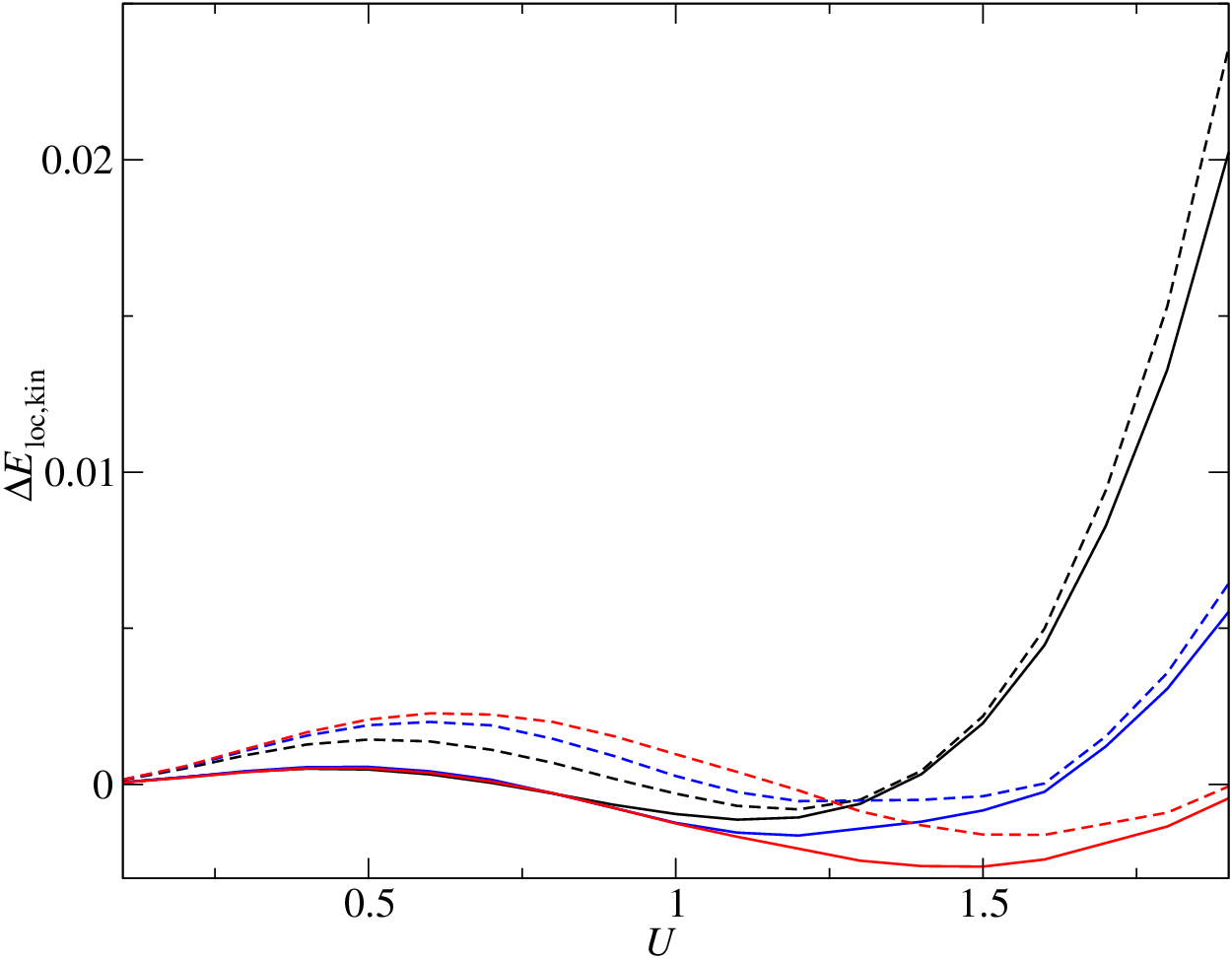
In Fig. 1 we display $\Delta E_{\rm kin}\equiv-(E_{\rm kin}^{\rm diag}-E_{\rm kin}^{\rm full})$ and $\Delta E_{\rm loc}\equiv E_{\rm loc}^{\rm diag}-E_{\rm loc}^{\rm full}$ for three different values of $\Delta$. Although the differences in these energies are clearly discernible, they are actually relatively small because $E_{\rm kin}$ is of the order of unity. This holds in particular for the differences in the total energy $\Delta E$ (not shown). Since we reversed the sign in the kinetic energy curve, $\Delta E$ is given as the (small) difference between solid and dashed lines in Fig. (1), $\Delta E=\Delta E_{\rm loc}-\Delta E_{\rm kin}$; the energy gain by using the full set of variational parameters is seen to be of the order of ${\cal O}(10^{-3})$, an order of magnitude smaller than the differences in kinetic and local energies.

The success of the diagonal form of the Gutzwiller correlator hinges on the proper choice of the basis states $|\Gamma\rangle$. They are formed with a crystal-field in $\epsilon_{\sigma,\sigma^{\prime}}$ for the generic $t_{2{\rm g}}$ orbitals $\phi_{xy}\sim xy$, $\phi_{xz}\sim xz$, and $\phi_{yz}\sim yz$ for $b=1,2,3$. The results for the energies are less good when we work with basis states $|\Gamma\rangle$ that are less appropriate. To illustrate this point, we introduce a rotated crystal field so that the single-electron orbitals are given by

and the new multiplet states $|\Gamma\rangle$ are formed using these single-particle orbitals orbitals. Note that we keep $\tilde{\eta}$ diagonal in the original $t_{2{\rm g}}$-basis in the calculation of $|\Psi_{0}\rangle$ via eq. (17) so that the single-particle band states and the local single-particle orbitals are not aligned anymore. Consequently, as seen from Fig. 2, the differences in the kinetic and local energies from the diagonal and the full variational Ansatz are larger than in the aligned case, by an order of magnitude. Correspondingly, the total variational energy decreases by several percent when we use the full variational-parameter matrix.

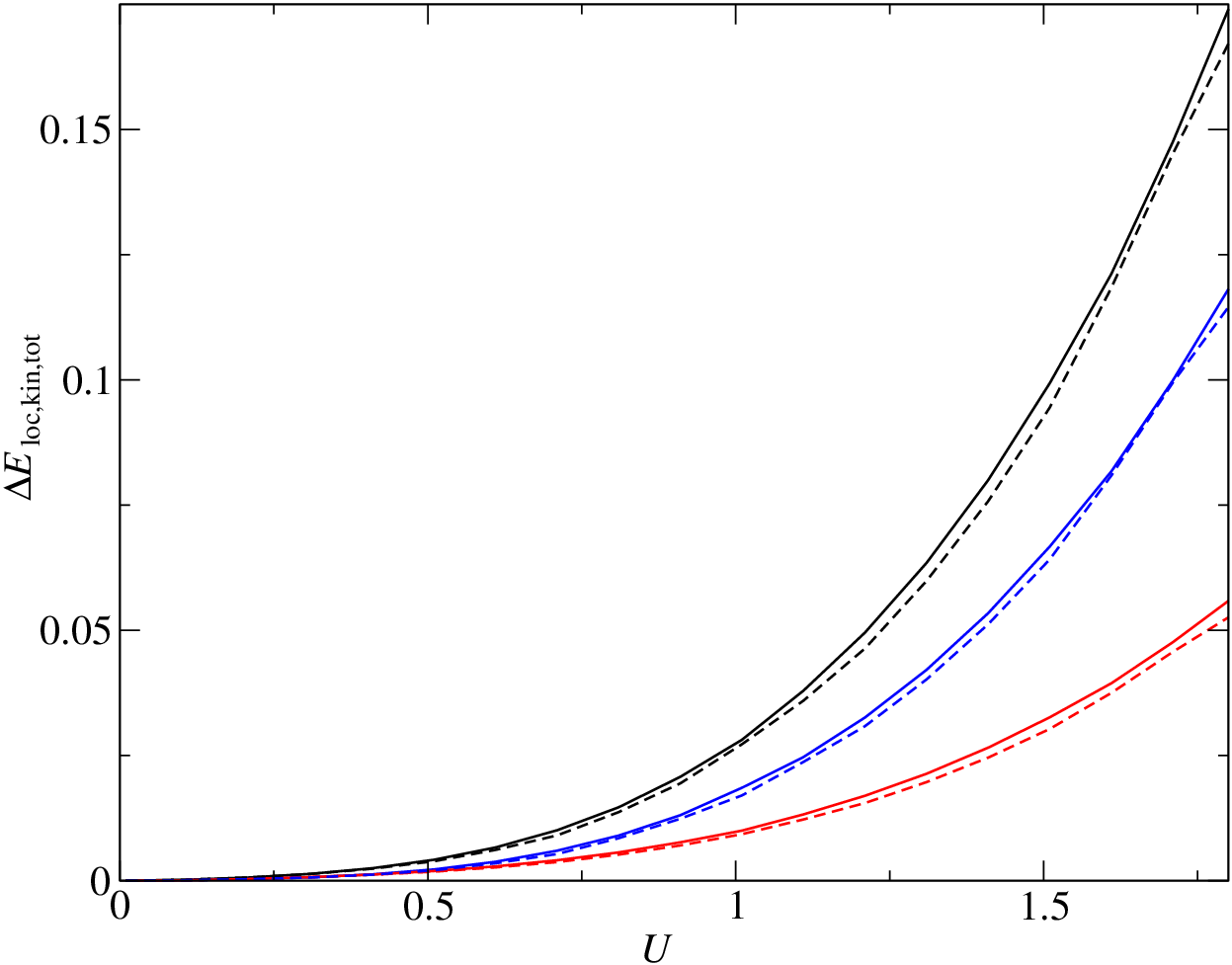
As a first step to improve the variational energies we can introduce non-diagonal variational parameters in the single-particle subspace of the atomic Hamiltonian where $|\Gamma\rangle$ contains only a single electron. The dashed lines in Fig. 2 show the corresponding results for this minimization. As the total energy must improve, the dashed red curve is always below the solid red line. However, the improvement using these additional non-diagonal parameters is marginal. Nevertheless, the inclusion of these terms has a very positive effect on the convergence of our minimization algorithm, as we shall explain now.

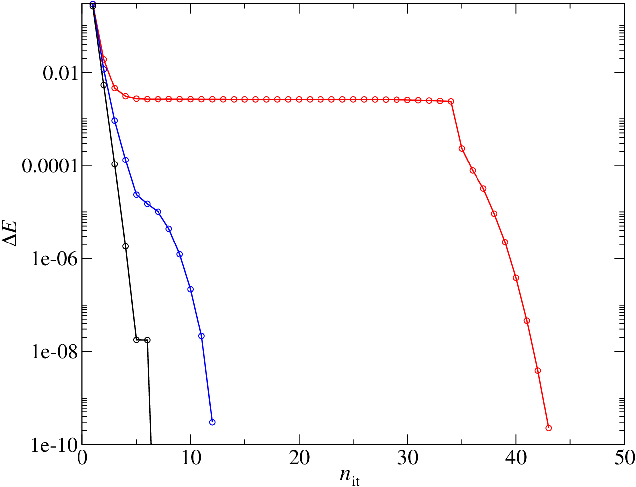
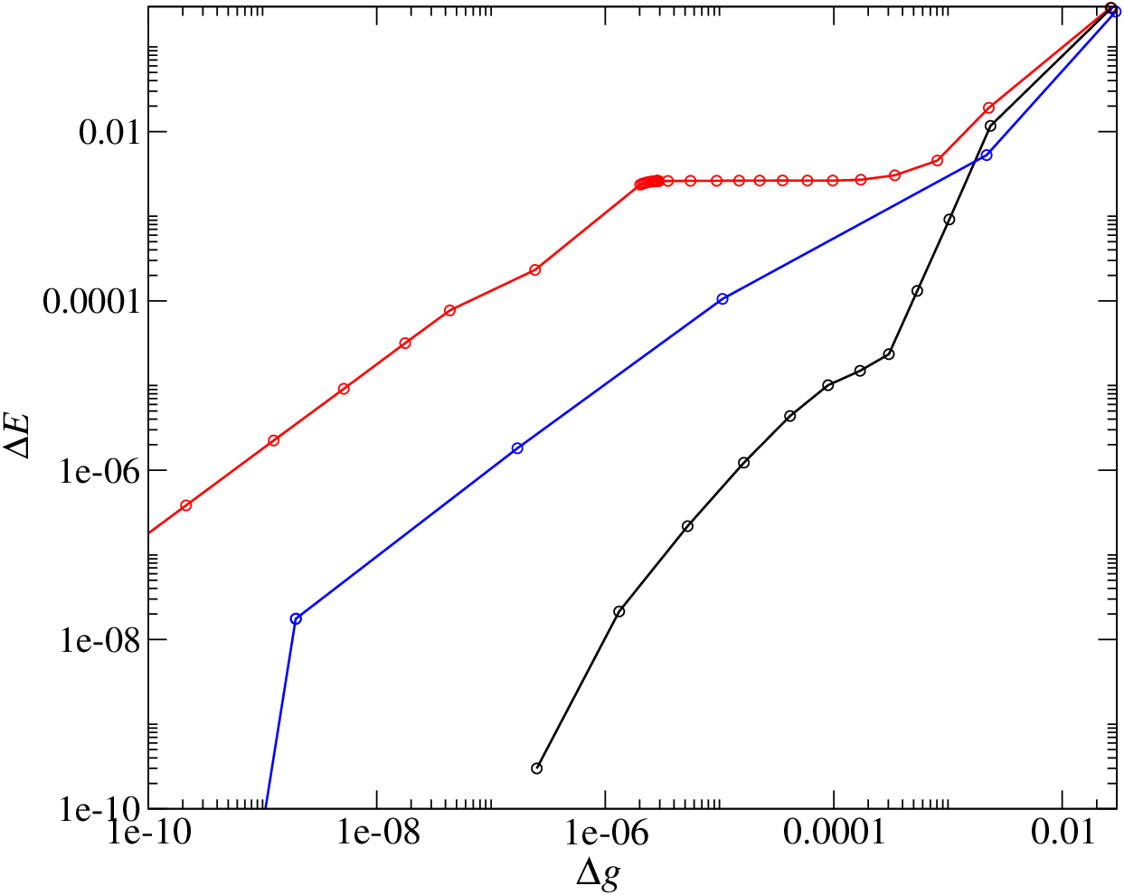
Figure 3 shows, on a logarithmic scale, the convergence of the energy expectation value towards its ground-state value at each step of the minimization algorithm for all three sets of variational-parameter matrices. Apparently, the convergence with a diagonal variational-parameter matrix is very slow when compared to the other two calculations. The main problem with our diagonal matrix is the satisfaction of the constraints (14) and (15). In our ‘Penalty and Augmented Lagrangian Method’ (PALM) [22, 23] we have to reach quite large values of the penalty parameter $\mu$ before the constraints fall below a certain threshold. This can be seen in Fig. 4 where we show the same energies as in Fig. 3, now as a function of the constraint mismatch parameter $\Delta g$ from eq. (18).

Our investigation of the crystal-field splitting shows that in low-symmetry situations we face two problems when we try not to take into account all elements of the Gutzwiller variational-parameter matrix.

• (i)

   The convergence of the minimization algorithm becomes worse, i.e., it takes more iteration steps to reach convergence.

• (ii)

   The expectation value for the variational ground-state energy noticeably increases. In the worst case, this indicates that the variational state is not flexible enough to describe quantitatively (or even qualitatively) the physics of the underlying Hamiltonian.

Our somewhat artificial example to reduce the local symmetry suggests two possible strategies to solve these problems.

• (i)

   To speed up the convergence, take into account a sufficient number of non-diagonal variational parameters in order to satisfy the constraints.

• (ii)

   Choose a proper basis set of multiplet states $|\Gamma\rangle$.

In the following section we shall test our strategies against the case where we reduce the symmetry by including the spin-orbit coupling in our local Hamiltonian.

The spin-orbit coupling provides a physical mechanism that lowers the symmetry of our model with degenerate $t_{2{\rm g}}$ orbitals. Since it influences the local orbitals, it is an important perturbation and requires a large flexibility in the Gutzwiller wave function. At the same time, it generates small quantitative corrections in the ground-state energy so that the Gutzwiller wave function must be evaluated with high numerical accuracy. The physics of such a system is discussed in detail in Ref. [22]. We will therefore concentrate in the following on the technical problem of convergence and accuracy of our energy minimization.

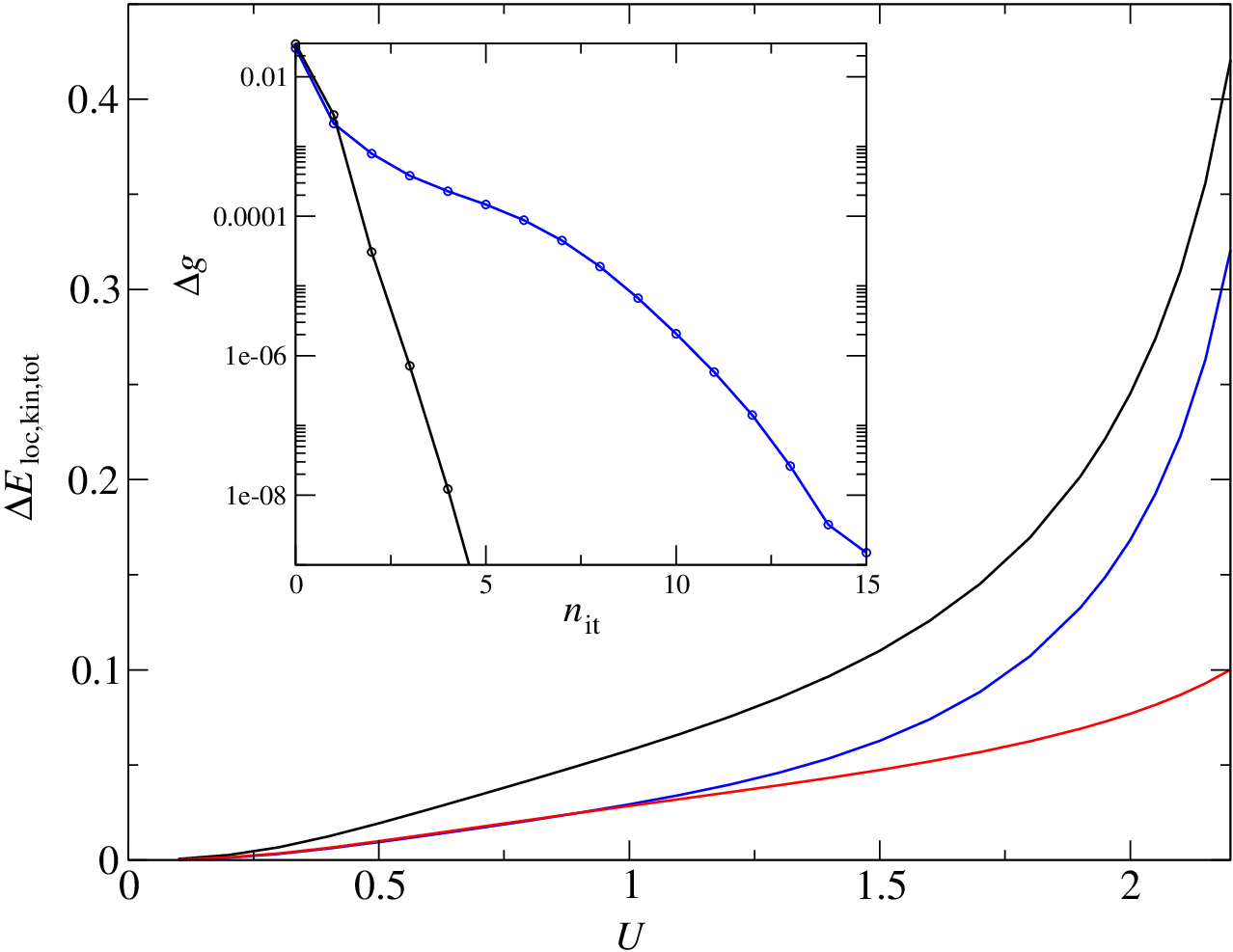
In the presence of the spin-orbit coupling, the six local spin-orbital states split into two-fold ($j=1/2$) and four-fold ($j=3/2$) degenerate sub-spaces. Similar splittings occur in the multiplet states $|\Gamma\rangle$. Since most of these states remain degenerate, we have to make a certain choice of our basis $|\Gamma\rangle$ when we work with a diagonal variational-parameter matrix. It turns out, however, that in the present calculations this choice is not significant, i.e., we obtain hardly any energy gain by optimizing the energy with respect to the basis $|\Gamma\rangle$.

In any case, the discrepancies in energy can be profound, of the order of ten percent for $U=2$, when we compare results for the full and a diagonal variational-parameter matrix. This can be seen in Fig. 5 where we show the energy differences defined in the previous section for a bare spin-orbit coupling of $\zeta=0.2$ [22]. As in our crystal-field calculations in Sect. 3.1, this inaccuracy goes hand in hand with a significantly slower convergence of the minimization algorithm, see the inset of Fig. 5.

As seen from the figure, the discrepancies in the kinetic and potential energies are much worse than those for the total energy. For the kinetic energy, this is reflected by rather different values for the band-width renormalization factors. For example, at $U=2$, the renormalizations are ($q^{2}_{1/2}\approx 0.72$, $q^{2}_{3/2}\approx 0.64$) for a diagonal variational-parameter matrix and ($q_{1/2}^{2}\approx 0.62$, $q_{3/2}^{2}\approx 0.61$) for the full variational-parameter matrix. These values do not change much when we carry out a full minimization also with respect to $|\Psi_{0}\rangle$. The corresponding numbers are ($q^{2}_{1/2}\approx 0.73$, $q^{2}_{3/2}\approx 0.64$) and ($q^{2}_{1/2}\approx 0.62$, $q^{2}_{3/2}\approx 0.60$), respectively. Therefore, the large differences in the band-width renormalization factors are not compensated by optimizing the corresponding single-particle states $|\Psi_{0}\rangle$. The results are generic for a full or only partial treatment of the variational-parameter matrix.

Moreover, in both cases the effective spin-orbit coupling in $\hat{H}_{0}^{\rm eff}$ [22] is quite different, $\bar{\zeta}^{\rm diag}\approx 0.35$ and $\bar{\zeta}^{\rm full}\approx 0.22$. As a consequence, the quasi-particle bandstructures that result from the two calculations [24] differ considerably, with respect to their band-widths and their spin-orbit splittings at various high-symmetry points in the Brillouin zone, see Fig. 6.

The example of the spin-orbit coupling corroborates our findings in Sect. 3.1 that the variational state with a diagonal variational-parameter matrix is not flexible enough to describe the physics of the underlying Hamiltonian.

A natural numerical approach to the problem is the inclusion of only a subset of non-diagonal variational parameters $\lambda_{\Gamma,\Gamma^{\prime}}$. Then, it arises the question how to select the parameters that are taken into account. We have tested two different conditions (CON1 and CON2), where we include all parameters for which

Here, we introduced the local expectation value

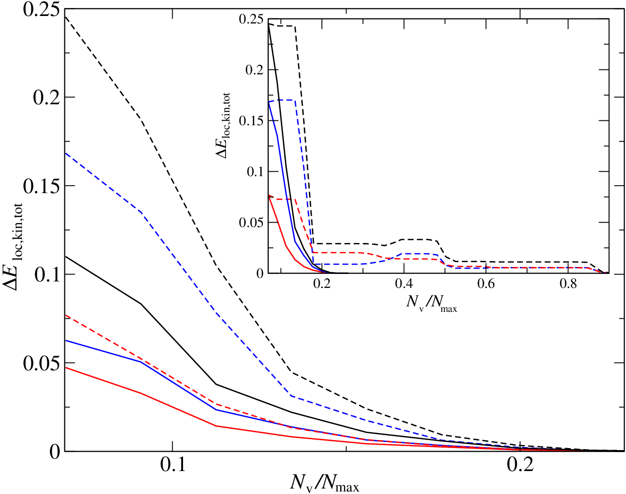
Figure 7 shows the errors in kinetic, local and total energy for $U=1.5,2$, $J/U=0.2$, and $\zeta=0.1,0.2$ as a function of the ratio $N_{\rm v}/N_{\rm max}$ of included variational parameters and their maximum number $N_{\rm max}=924$. Clearly, the method CON1 converges quite rapidly as a function of $N_{\rm v}/N_{\rm max}$. Already $20\%$ of the parameters are sufficient to get a very good agreement with the full calculation. The convergence of CON2 is much worse as can be seen in the inset of Fig. 7.

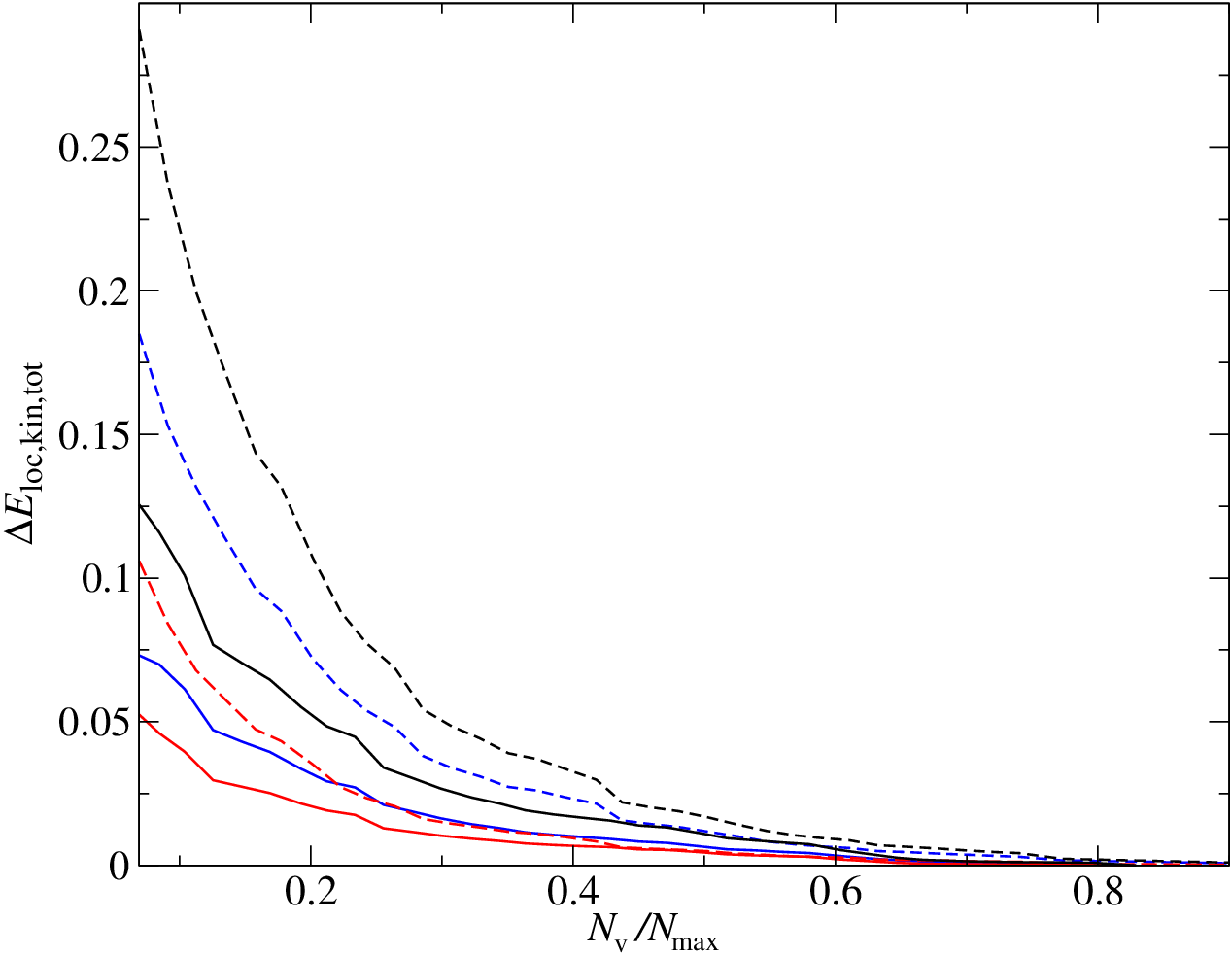
The much better convergence of CON1 does not come as a surprise. The point symmetry of the system is still relatively high so that many variational parameters $\lambda_{\Gamma,\Gamma^{\prime}}$ do not enter the energy functional at all. Such parameters are identified automatically and excluded by CON1 because for them we have $m^{0}_{\Gamma,\Gamma^{\prime}}=0<m_{\rm c}$. In fact, when we lower the symmetry further by introducing an additional crystal field as in Sect. 3.1, the performance of CON1 is less impressive. This can be seen from Fig. 8 where we show the errors in energies for $U=2$, $J/U=0.2$, $\zeta=0.2$, and a crystal-field splitting $\Delta=0.2$.

As seen from Fig. 8, the brute-force inclusion of a maximal number of non-diagonal variational parameters may still lead to significant errors in low-symmetry systems with orbital number $n_{\rm o}>3$. Moreover, unlike in our three-band model, there is no way to estimate systematically the error that is caused by the neglect of some non-diagonal parameters. In the following we develop a more sophisticated algorithm which addresses both of these problems.

If we knew the eigenstates $|\Gamma_{d}\rangle_{i}$ of the optimum Gutzwiller correlation operator in (11) we would obtain the minimal Gutzwiller ground-state energy by working with a correlation operator that depends only on (in our case $64$) diagonal variational parameters. Therefore, it is highly desirable to have an algorithm which systematically improves our multiplet basis $|\Gamma\rangle$ towards $|\Gamma_{d}\rangle$ in order to make non-diagonal variational parameters increasingly dispensable. To achieve this, we perform the following steps.

• (i)

   Start with some initial local multiplet basis $|\Gamma_{0}\rangle$.

• (ii)

   Minimize the energy with respect to a variational-parameter matrix that contains a subset of non-diagonal parameters.

• (iii)

   Determine the eigenstates $|\Gamma_{1}\rangle$ of the optimum variational-parameter matrix $\tilde{\lambda}$ obtained in step (ii).

• (iv)

   Set $|\Gamma_{0}\rangle=|\Gamma_{1}\rangle$ and go back to step (ii) until the variational ground-state energy does not improve significantly anymore.

As an illustration, we apply this algorithm to the system with spin-orbit coupling and crystal-field splitting that we analyzed in Fig. 8. As subsets in step (ii), we choose variational parameters that belong to the subspaces with particle numbers $n_{\rm active}=3$, $n_{\rm active}=2,4$, or $n_{\rm active}=1,5$.

In table 1 we present the error $\Delta E_{\rm tot}$ after each step of the iteration, and the corresponding required CPU time $t_{\rm CPU}$, relative to the CPU time $t^{\rm full}_{\rm CPU}$ for a full Gutzwiller minimization. For comparison, we also show the CPU time $t^{\rm CON1}_{\rm CPU}$ of some CON1 minimizations that lead to the same accuracy, cf. the red dashed line in Fig. 8.

Note that the not strictly-monotonic behavior of $t^{\rm CON1}_{\rm CPU}$ in table 1 is genuine. While the CPU time for the ‘Broyden-Fletcher-Goldfarb-Shanno’ (BFGS) minimization’ with respect to $\tilde{\lambda}$ generally increases with the total number $N_{\rm v}$ of variational parameters, the constraint enforcing ‘Penalty and Augmented Lagrangian method’ (PALM) contains a certain degree of arbitrariness, see Ref. [22]. Therefore, it can occasionally happen that, when increasing $N_{\rm v}$, the PALM scheme needs less loops. This can compensate the increase of $T^{\rm CON1}_{\rm CPU}$ from the BFGS minimization.

Table 1 shows that the convergence of our algorithm is rather fast, especially in the first few steps where the energy makes large gains with modest numerical effort. Only when we try to obtain very, and probably unnecessarily, accurate results, it will eventually be outperformed by a CON1 minimization.

Our algorithm overcomes the computer memory barrier of the CON1 method because its accuracy depends on the allocated CPU time. Most importantly, the iterative algorithm can be expected to converge for any multi-orbital system. Therefore, we think that it is the most promising candidate to be used for a general Gutzwiller minimization code that is needed in a Gutzwiller-DFT program package [27, 28, 29].

References

- [1] G. R. Stewart, Rev. Mod. Phys. 83, 1589 (2011).
- [2] P. Dai, Rev. Mod. Phys. 87, 855 (2015).
- [3] O. Andersen and L. Boeri, Annalen der Physik 523, 8 (2011).
- [4] M. Gutzwiller, Phys. Rev. Lett. 10, 159 (1963).
- [5] M. Gutzwiller, Phys. Rev. 134, A923 (1964).
- [6] W. Metzner and D. Vollhardt, Phys. Rev. Lett. 59, 121 (1987).
- [7] F. Gebhard, Phys. Rev. B 41, 9452 (1990).
- [8] T. Schickling, F. Gebhard, and J. Bünemann, Phys. Rev. Lett. 106, 146402 (2011).
- [9] T. Schickling, F. Gebhard, J. Bünemann, L. Boeri, O. K. Andersen, and W. Weber, Phys. Rev. Lett. 108, 036406 (2012).
- [10] J. Bünemann, T. Schickling, and F. Gebhard, Europhys. Lett. 98, 27006 (2012).
- [11] J. Kaczmarczyk, J. Spałek, T. Schickling, and J. Bünemann, Phys. Rev. B 88, 115127 (2013).
- [12] J. Kaczmarczyk, Phil. Mag. 95, 563 (2015).
- [13] J. Kaczmarczyk, T. Schickling, and J. Bünemann, physica status solidi (b) 252, 2059 (2015).
- [14] M. M. Wysokiński, J. Kaczmarczyk, and J. Spałek, Phys. Rev. B 92, 125135 (2015).
- [15] M. M. Wysokiński, J. Kaczmarczyk, and J. Spałek, arxiv: 1510.00224.
- [16] J. Kaczmarczyk, J. Bünemann, and J. Spałek, New Journal of Physics 16, 073018 (2014).
- [17] K. zu Münster and J. Bünemann, (unpublished).
- [18] J. C. Slater and G. F. Koster, Phys. Rev. 94, 1498 (1954).
- [19] J. Bünemann, W. Weber, and F. Gebhard, Phys. Rev. B 57, 6896 (1998).
- [20] J. Bünemann, F. Gebhard, and W. Weber, in: Frontiers in Magnetic Materials, edited by A. Narlikar, (Springer, Berlin, 2005).
- [21] J. Bünemann, F. Gebhard, T. Schickling, and W. Weber, physica status solidi (b) 249, 1282 (2012).
- [22] J. Bünemann, T. Linneweber, U. Löw, F. Anders, and F. Gebhard, arXiv:1603.07544 (2016).
- [23] J. Nocedal and S. J. Wright, Numerical Optimization, 2nd edition (Springer, New York, 2006).
- [24] J. Bünemann, F. Gebhard, and R. Thul, Phys. Rev. B 67, 75103 (2003).
- [25] G. Borghi, M. Fabrizio, and E. Tosatti, Phys. Rev. B 90, 125102 (2014).
- [26] L. Du, L. Huang, and X. Dai, Eur. Phys. J. B 86, 94 (2013).
- [27] K. M. Ho, J. Schmalian, and C. Z. Wang, Phys. Rev. B 77, 073101 (2008).
- [28] X. Deng, X. Dai, and Z. Fang, Europhys. Lett. 83, 37008 (2008).
- [29] T. Schickling, J. Bünemann, F. Gebhard, and W. Weber, New Journal of Physics 16, 93034 (2014).