Density matrix renormalization group study in energy space for a single-impurity Anderson model and an impurity quantum phase transition
Abstract
The density matrix renormalization group method is introduced in energy space to study Anderson impurity models. The method allows for calculations in the thermodynamic limit and is advantageous for studying not only the dynamical properties but also the quantum entanglement of the ground-state at the vicinity of an impurity quantum phase transition. This method is applied to obtain numerically exactly the ground-state phase diagram of the single-impurity Anderson model on the honeycomb lattice at half-filling. The calculation of local static quantities shows that the phase diagram contains two distinct phases, the local moment (LM) phase and the asymmetric strong coupling (ASC) phase, but no Kondo screening phase. These results are supported by the local spin and charge excitation spectra, which exhibit qualitatively different behavior in these two phases and also reveal the existence of the valence fluctuating point at the phase boundary. For comparison, we also study the low-energy effective pseudogap Anderson model using the method introduced here. Although the high-energy excitations are obviously different, we find that the ground-state phase diagram and the asymptotically low-energy excitations are in good quantitative agreement with those for the single-impurity Anderson model on the honeycomb lattice, thus providing a quantitative justification for the previous studies based on low-energy approximate approaches. Furthermore, we find that the lowest entanglement level is doubly degenerate for the LM phase, whereas it is singlet for the ASC phase and is accidentally three fold degenerate at the valence fluctuating point. This should be contrasted with the degeneracy of the energy spectrum because the ground-state is found to be always singlet. Our results therefore clearly demonstrate that the low-lying entanglement spectrum can be used to determine with high accuracy the phase boundary of the impurity quantum phase transition.
pacs
75.20.Hr, 73.22.Pr, 75.30.HxI Introduction
Recent experiments have revealed that the introduction of adatoms induces the local magnetic moments in graphene [1, 2]. One of the simplest models describing the magnetic impurity problem in graphene is an Anderson impurity coupled to the conduction electrons on the honeycomb lattice with the massless Dirac energy dispersion which results in the linear density of states () around the Fermi level [3]. This problem is known as the pseudogap Kondo problem [4] and has been studied extensively for over a decade by the renormalization group analysis [5, 6] and the numerical renormalization group (NRG) method [7, 8, 9, 10, 11]. These previous studies have already found that, at zero temperature, there exit two phases, i.e., the local moment (LM) phase and the asymmetric strong coupling (ASC) phase, and the phase boundary corresponds to the valence fluctuating (VF) point [7].
These studies are, however, based on the low-energy effective pseudogap Anderson models [4] and focused mostly on the two special cases in the large conduction band limit and in the strong coupling limit [7, 8, 9, 10]. Although the essential part of Kondo physics should be captured in these low-energy analyses, it is rather surprising that the phase diagram even for the simplest and most fundamental Anderson impurity model, not for the low-energy effective models, has not been established so far. The reason is simply because of lack of reliable numerical methods which can treat Anderson impurity models numerically exactly in two and three spatial dimensions. Establishing the numerically exact ground state phase diagram of the Anderson impurity model is also beneficial to the previous studies based on the low-energy effective models since it can provide a strong justification for their approximations.
On the other hand, the entanglement spectrum [12] has attracted much attention recently in condensed matter physics for identifying topologically ordered phases [12, 13, 14, 15, 16]. In these systems, the degeneracy of the low-lying entanglement spectrum is intimately related to the existence of the surface boundary states which are protected by bulk symmetries. Since the magnetic impurity problem can be regarded as a boundary problem in one dimension [17], it is also valuable to explore its quantum entanglement aspects. In this context, the recent study of a “spin-only” version of a two-impurity Kondo model has shown that the gap of the entanglement spectrum can be regarded as an order parameter [18]. The entanglement spectrum is thus expected to be also used to quantify different quantum phases in magnetic impurity models including Anderson impurity models [19].
The main purposes of this paper are threefold. First, we introduce a numerical method which enables us to treat exactly general Anderson impurity models in any spatial dimension in the thermodynamic limit. Secondly, we demonstrate the method developed here by applying it to one of the simplest Anderson impurity models in two spatial dimensions and compare the results with those for the low-energy effective pseudogap Anderson model. Third, we explore the impurity quantum phase transition and the low-lying entanglement spectrum to uncover the degeneracy of the lowest entanglement level across the impurity quantum phase transition.
To this end, here we introduce the density matrix renormalization group (DMRG) method [20, 21] for general Anderson impurity models represented in energy space. This method is applied to the single-impurity Anderson model on the honeycomb lattice at half-filling to determine precisely the ground-state phase diagram in a wide range of parameters, including an intermediate coupling region. The calculations of the local static quantities reveal that the phase diagram contains only two phases, i.e., the LM and ASC phases. The local spin and charge excitation spectra further support these results and also show the existence of the VF point at the phase boundary. We also study the low-energy effective pseudogap Anderson model and compare the ground-state phase diagram as well as the local spin and charge excitation spectra with those for the single-impurity Anderson model on the honeycomb lattice. Although the high-energy excitations are apparently different, the ground-state phase diagrams and the asymptotically low-energy excitations for these two models are found to be in excellent quantitative agreement. Moreover, we find that the degeneracy of the lowest entanglement level is different in the three different regions of the phase diagram, i.e., the LM and ASC phases and the VF point. This is in sharp contrast to the degeneracy of the ground state, which is found always singlet in all three regions. Although it has been pointed out that the sudden change of entanglement properties is not always related to quantum phase transition [22], our results demonstrate that the low-lying entanglement spectrum can be used to determine the impurity quantum phase transition, at least, between the LM and ASC phases.
The rest of this paper is organized as follows. First, the single-impurity Anderson model on the honeycomb lattice and the corresponding low-energy effective pseudogap Anderson model are introduced in Sec. II. The DMRG method to solve general Anderson impurity models in energy space is also described in details in Sec. II. The numerical results for the single-impurity Anderson model on the honeycomb lattice are shown in Sec. III. Based on the local static properties shown in Sec. III.2, the ground-state phase diagram is established in Sec. III.3. The local spin and charge excitation spectra are also calculated in Sec. III.4 to support the phase diagram. Furthermore, these results are compared with those for the low-energy effective pseudogap Anderson model in Sec. III.5. Finally, the low-lying entanglement spectrum and the entanglement entropy for the single-impurity Anderson model on the honeycomb lattice are discussed in Sec. III.6 before summarizing the paper in Sec. IV. The energy space description of the single-impurity Anderson model is discussed in Appendix A and the further technical details of numerical calculations are provided in Appendix B.
II Models and Method
In this section, we first introduce the single-impurity Anderson model on the honeycomb lattice. Considering this model as an example, we describe in details the DMRG method in energy space, which can treat exactly general Anderson impurity models in any spatial dimensions. We also introduce the pseudogap Anderson model as a low-energy effective model for the single-impurity Anderson model on the honeycomb lattice.
II.1 Single-impurity Anderson model
In order to be specific and also because it is one of the simplest models for the magnetic impurity problem in graphene, here we consider the single-impurity Anderson model on the honeycomb lattice [see Fig. 1(a)] defined by the following Hamiltonian:
| (1) |
where the impurity Hamiltonian , including the on-site Coulomb interaction and the on-site potential at the impurity site, is given as
| (2) |
the conduction band with the nearest-neighbor hopping is described on the honeycomb lattice as
| (3) |
and the hybridization between the impurity site and the conduction band is represented as
| (4) |
Here, () is the creation (annihilation) operator of a conduction electron with spin at site on the honeycomb lattice and () is the creation (annihilation) operator of an electron at the impurity site with and . The sum in denoted by runs over nearest-neighbor pairs of conduction sites and on the honeycomb lattice. Notice here that the impurity site is connected to only one of the conduction sites at through the hybridization in , as shown in Fig. 1(a). The electron density is set to be half-filled, i.e., .

II.2 DMRG method in energy space
We first describe the Hamiltonian in energy space. This can be done by noticing that the effective action of the impurity site for can be reproduced exactly by, e.g., the following Hamiltonian:
| (5) | |||||
where () is the creation (annihilation) operator of a conduction electron which represents the eigenstate of with energy and spin , and the local density of state per spin for the conduction band is denoted as [7, 8]. The equivalence between and is shown in Appendix A.
Next, we discretize the energy with the logarithmic discretization scheme
| (6) |
where is the conduction band width ( for the conduction band described by ), is a parameter which sets a series of intervals in ’s with [23], and we set . Defining a representative fermion operator () for each energy interval between and , the Hamiltonian can now be expressed as
| (7) | |||||
where
| (8) |
and
| (9) |
This discretization scheme is similar to the one employed in the NRG method [24]. The local density of states for the conduction band can be calculated with desired accuracy by employing the linear tetrahedron method, as shown in Fig. 2 [25, 26].

Since we can use any discretization scheme to discretize the energy , we also introduce the constant discretization scheme
| (10) |
with . The logarithmic discretization scheme has much denser energy meshes as approaches to zero, but has much less energy meshes for larger away from zero. Therefore, in order to treat correctly the band structure in high-energy scales, the logarithmic discretization scheme requires small close to 1, which is computationally demanding. In contrast, the constant discretization scheme distributes the energy meshes equally for all energy scales. We find that the logarithmic discretization scheme is suitable for the calculation of static quantities but the constant discretization scheme is better computationally to calculate dynamical quantities specially when the high-energy excitations are involved (see Appendix B for more details). It is also shown in Appendix A that the effective action of the impurity site for in both discretization schemes is exactly the same as the one for .
Finally, we transform the Hamiltonian into a one-dimensional form with no long-range hopping terms but keeping the interaction term local. For this purpose, we apply the Lanczos iteration [27] to the second and third terms in the right-hand side of with choosing the impurity site as the initial Lanczos basis vector. Introducing the vector representation of the electron creation and annihilation operators, e.g.,
| (11) | |||||
can be represented as
| (12) |
where is a matrix defined as
Notice here that although the interaction term at the impurity site is described by the same impurity Hamiltonian , introduces long-range hopping terms as the impurity site is hybridized with all conduction sites in energy space. This is usually problematic for DMRG calculations. As shown below, this can be completely alleviated by the Lanczos basis transformation without introducing additional long-range interaction terms for .
Taking as the initial Lanczos basis the -dimensional column unit vector with the th element
| (24) |
we can generate the Lanczos basis via the three-time recurrences
| (25) |
for with and , where
| (26) |
and
| (27) |
i.e., the norm of the -dimensional column vector in the right-hand side of Eq. (25).
Using these Lanczos bases , can be transformed into the following tridiagonal matrix:
and accordingly the electron creations operators are transformed into the new operators as
| (36) |
with . Since and , one can easily show that . Therefore, the new operators and satisfy the fermion anticommutation relations, e.g., . Note also that as .
The resulting Hamiltonian after this basis transformation is
| (37) | |||||
Notice first that the impurity site is described by the same local Hamiltonian as in and therefore the interaction term remains local. On the other hand, the hopping terms are now all short ranged with only nearest-neighbor hopping . Therefore, the model described by is a simple one-dimensional system of sites, as schematically shown in Fig. 1(b), and can be best treated by the DMRG method [20, 21, 28, 29].
Four remarks are in order regarding the method introduced here. First, as it is well known in the standard Lanczos method [27], the transformation from to is exact only when , assuming that is not contained in an invariant subspace and thus the Lanczos iteration is not terminated before generating . Only in this case, and thus
| (38) |
as is a orthogonal matrix.
Second, it is apparent from the construction that this method is for calculations in the thermodynamic limit. and also in the logarithmic discretization scheme determine the energy resolution as well as the model parameters and in . Therefore, these quantities and control the accuracy of with respect to in the thermodynamic limit. In principle, the logarithmic discretization scheme becomes exact when and , where is positive infinitesimal. Similarly, the constant discretization scheme becomes exact when . However, as discussed in Appendix B, we find that reasonably large and (but ) can well represent the thermodynamic limit (provided that is sufficiently small for the logarithmic discretization scheme).
Third, the single-impurity Anderson model in two spatial dimensions is considered here. This is only to simplify the explanation of the method introduced here. The extension of the method to more general cases such as a two-impurity Anderson model and a multiorbital many-impurity Anderson model is rather straightforward by using the block Lanczos technique [30]. Indeed, the similar transformation for Anderson impurity models in real space and its extension to multiorbital systems are found in Refs. [30, 31, 32]. The extension to three-dimensional systems is also straightforward.
Fourth, the method is similar to the NRG approach [24] in that both treat Anderson impurity models represented in energy space. Indeed, the logarithmic discretization scheme is employed in the NRG method, where corresponds to the number of renormalization iterations [24]. However, these two approaches are conceptually different because the DMRG method optimizes the wave function based on the largest eigenstates of the reduced density matrix for that wave function, while the NRG method constructs the low-energy effective Hamiltonian based on the lowest eigenstates of the Hamiltonian. Note also that the method introduced here can take into account the band structure effect accurately over large energy scales, in contrast to the low-energy approximate approaches. This is obviously important when high-energy excitations are discussed.
II.3 Pseudogap Anderson model
It is valuable to compare the results for the single-impurity Anderson model on the honeycomb lattice with those for the corresponding pseudogap Anderson model. The pseudogap Anderson model is described by Hamiltonian or with the following local density of states per spin for the conduction band (see Fig. 2):
| (39) |
This local density of states is directly used for in Eqs. (5) and (7) to construct , which then can be solved by the DMRG method, as described above. The asymptotic behavior of for the conduction band on the honeycomb lattice described by is
| (40) |
for around zero [3]. Therefore, by setting the band width for the pseudogap Anderson model as , can reproduce exactly the asymptotic behavior of for the conduction band on the honeycomb lattice, as shown in Fig. 2.
The pseudogap Anderson model and its strong coupling counterpart, i.e., the pseudogap Kondo model, have been studied extensively using the analytical and NRG methods [4, 5, 6, 7, 8, 9, 10, 11]. The ground-state phase diagram of the pseudogap Anderson model has two distinct phases, the LM phase and the ASC phase, and the VF point at the phase boundary [7]. In the LM phase, a free local moment at the impurity site survives without Kondo screening even at zero temperature. The fixed point of this phase can be characterized as with [7], i.e., the free local moment being decoupled from the conduction band. In the ASC phase, the fixed point is characterized as for , and for [7]. Since the two electrons (two holes) occupy the impurity site for (), no local moment is formed. The fixed point for the VF point is characterized as for and with for [7]. Since the impurity site is decoupled from the conduction band, the ground state is threefold degenerate due to three different local states at the impurity site, i.e., the empty state and the singly occupied states with up or down electron for .
III Results
We first summarize briefly the conditions employed for the numerical calculations before discussing the numerical results for the single-impurity Anderson model on the honeycomb lattice. These results are then compared with those for the pseudogap Anderson model. We also examine the entanglement spectrum for the ground state of the single-impurity Anderson model on the honeycomb lattice to characterize the impurity quantum phase transition.
III.1 Numerical details
We set that (even) in Eq. (37) throughout the calculations discussed here, unless otherwise stated. As already explained in Sec. II.2, (and also when the logarithmic discretization scheme is used) controls the energy resolution and can be taken to be up to . Therefore, in principle, one should take the infinite limit of and along with for the logarithmic discretization scheme. However, we find that the quantities studied here are well converged for sufficiently large but finite values of and with keeping a fixed ratio of , at least, when the logarithmic discretization scheme with as small as 1.15 is used (see Appendix B). Therefore, we take up to with the component of total spin and keep largest eigenstates of the reduced density matrix in the DMRG calculations.
When the logarithmic discretization scheme is used, the discarded weights are found to be significantly small, typically of the order –. The corresponding error of the ground-state energy is as small as , which is even smaller than the smallest level spacing of the eigenvalues for in Eq. (II.2) with . When the constant discretization scheme is used, the discarded weights are as small as and the corresponding error of the ground-state energy is about . We employ the logarithmic discretization scheme to calculate the static quantities as well as the entanglement spectrum and the constant discretization scheme to calculate the full excitation spectra (see Appendix B). However, to extrapolate the static limit of the dynamical quantity, we use the logarithmic discretization scheme with up to . It should be also noted that the ground state is found to be always singlet as long as is even and finite.
III.2 Local static quantities
Let us first calculate the local density per spin at the impurity site
| (41) |
and the total spin at the impurity site
| (42) |
where is the ground state and the spin operator at the impurity site is given as
| (43) |
with being Pauli matrices. Note that because of symmetry of and .

As shown in Fig. 3, we find that these quantities change discontinuously at two distinct values of for given and . It should be emphasized, however, that these deceptively discontinuous changes are simply due to a finite grid size of used in the figures, but not due to the level crossing of two different states as often found in finite-size calculations. Indeed, we find in Fig. 4 that these quantities vary smoothly with when a much smaller grid size of is used. We also find in Fig. 4 that the change of these quantities becomes sharper and steeper with increasing . Therefore, we expect that it becomes truly discontinuous only when we take the limit of .

Nevertheless, the steep changes of these quantities imply that there are three phases for a given , a low-density phase () for small , an intermediate density phase () which includes the particle-hole symmetric limit with , and a high-density phase () for large . While the total spin is suppressed in the low- and high-density phases, it is enhanced in the intermediate density phase. It should be noticed here that the low- and high-density phases are related under the particle-hole transformation. This is because the model with a parameter set in particle picture can be transformed into the same model with in hole picture. Indeed, our results satisfy that () at the impurity potential is exactly the same as () at the impurity potential for given and . Together with the results of the spin and charge excitation spectra shown in Sec. III.3, we identify the intermediate density phase as the LM phase where the local moment is formed at the impurity site, and the low- and high-density phases as the ASC phase where essentially two holes or electrons occupy the impurity site with no local moment formed.
III.3 Ground-state phase diagram
Systematically calculating and for different values of , we obtain the ground-state phase diagram for the single-impurity Anderson model on the honeycomb lattice in a wide range of parameters, and . As shown in Fig. 5, the LM phase appears around the particle-hole symmetric limit with , where is exactly . The region of this phase is found to decrease with increasing . This is easily understood by considering that the increase of enhances the bonding between the impurity site and the conduction site , which then leads to the formation of the bond singlet state. Eventually, the LM phase exists only along the particle-hole symmetric line in the limit of . Our results in Fig. 5 also imply the absence of Kondo screening phase. This can be understood simply as the consequence of the characteristic density of states of the conduction band since the Kondo temperature [33]. The phase diagram is therefore in good qualitative agreement with that obtained by the low-energy approximate approaches [6, 7]. In fact, as discussed below in Sec. III.5, the phase diagram is found to be quantitatively compared with that for the pseudogap Anderson model.

III.4 Dynamical quantities
Next, we calculate the dynamical quantities to support the assignment of different phases found in the phase diagram. The dynamical quantities studied here are the spin excitation spectrum at impurity site
| (44) |
and the charge excitation spectrum at impurity site
| (45) |
where is the ground-state energy and is a broadening factor. We calculate these quantities using the dynamical DMRG method [34].
Figure 6 shows the spin excitation spectra for and . In this case, the transition occurs at –. As seen in Fig. 6, in the LM phase for increases as . In contrast, for is suppressed in the ASC phase for . The dependence of shown in the inset of Fig. 6 reveals that in the LM (ASC) phase increases (decreases) exponentially with for large , i.e.,
| (46) |
with the same in each phase, independent of values of , as summarized in Table 1. Therefore, we can safely conclude that
| (47) |
in the LM phase and
| (48) |
in the ASC phase. The divergent behavior of implies the presence of free local moment in the LM phases, while indicates no local moment at the impurity site in the ASC phase.

| LM phase | ASC phase | VF point | |
|---|---|---|---|
The charge excitation spectra are shown in Fig. 7. In contrast to , we find that for in both LM and ASC phases. This is more apparent in the dependence of , as shown in the inset of Fig. 7, because for large
| (49) |
with (also see Table 1), and thus
| (50) |
in the LM and ASC phases. However, for the exact phase boundary at , we find that as well as increases exponentially with (see the insets of Figs. 6 and 7, and also see Table 1), and therefore
| (51) |
and
| (52) |
suggesting the VF point. In the renormalization group analysis, the VF fixed point is characterized by the renormalized parameters (, , ) = (, , ) for [7]. Consequently, three local states at the impurity site, , , and , contribute equally to the threefold-degenerate ground state and thus both and diverge.

III.5 Results for the pseudogap Anderson model
Here, we compare the results of the local static quantities, the ground-state phase diagram, and the excitation spectra for the pseudogap Anderson model at half-filling, i.e., , to those for the single-impurity Anderson model on the honeycomb lattice discussed above.
Figure 8 shows the local density and total spin at the impurity site for the pseudogap Anderson model. We find in Fig. 8 that these local static quantities, including the phase boundaries where the abrupt changes of these quantities occur, for the pseudogap Anderson model are in quantitatively excellent agreement with those for the single-impurity Anderson model on the honeycomb lattice. Since the pseudogap Anderson model is a low-energy effective model for the single-impurity Anderson model on the honeycomb lattice, our results ensure that the low-energy effective description of the pseudogap Anderson model is quantitatively valid for these static quantities.

Systematically calculating and for different values of , we obtain in Fig. 9 the ground-state phase diagram for the pseudogap Anderson model. We find that the phase boundaries are almost identical to those for the single-impurity Anderson model on the honeycomb lattice. For instance, the VF point for and is located at – for the pseudogap Anderson model, which is comparable with – for the single-impurity Anderson model on the honeycomb lattice.

Figures 10 and 11 show the spin and charge excitation spectra at the impurity site, and , respectively. Comparing with Figs. 6 and 7, the line shapes of these excitation spectra are apparently different from those for the single-impurity Anderson model on the honeycomb lattice. However, as shown in the insets of Figs. 10 and 11, we find that the asymptotic behavior of these quantities around are qualitatively the same for both models, i.e., and in the LM phase, and in the ASC phase, and and at the VF point. Assuming that and diverge or decay exponentially for large , as in Eqs. (46) and (49), we can estimate the diverging or decaying factors and for the pseudogap Anderson model. As shown in Table 2, we find that the obtained and are indeed very close to those for the single-impurity Anderson model on the honeycomb lattice shown in Table 1, indicating that the asymptotically low-energy excitations of the single-impurity Anderson model on the honeycomb lattice are also well described by the low-energy effective pseudogap Anderson model.


| LM phase | ASC phase | VF point | |
|---|---|---|---|
III.6 Entanglement spectrum
Let us now discuss the entanglement spectrum for the ground state of the single impurity Anderson model on the honeycomb lattice. In the DMRG method, the system is divided into two parts, the left and right blocks, as shown in Fig. 1(b), with the sizes being and , respectively, i.e., . Thus, the wave function is generally represented as
| (53) |
where and indicate the bases of the left and right blocks, respectively. The reduced density matrix for the left block is
| (54) |
and the th eigenvalue of is denoted as in descending order, i.e.,
| (55) |
where is the number of density matrix eigenstates kept in the DMRG calculations. One can readily show that and when . The entanglement spectrum [12] is defined as
| (56) |
and hence
| (57) |
Figure 12 shows a low-lying part of for the ground state at the vicinity of the phase boundary. It is clear in Fig. 12(a) that the lowest and the first excited entanglement levels cross at . As shown in Fig. 12(b), we find that the lowest entanglement level for odd is doubly degenerate in the LM phase, singlet in the ASC phase, and accidentally three fold degenerate at , i.e., the VF point [35]. Because of the qualitatively different behavior, we can consider the gap of the entanglement spectrum
| (58) |
as an “order parameter” to distinguish the different phases in the phase diagram. As shown in Fig. 12(c), changes abruptly at for large and it is finite only when . Indeed, the phase boundary determined from is the same as the one estimated in Fig. 3. This clearly demonstrates that serves as a quantity to determine the phase boundary of the impurity quantum phase transition. We should emphasize here that the ground state is always singlet as long as is even and finite. Therefore, the similar characteristic feature of the degeneracy in the low-lying entanglement spectrum is absent in the low-lying energy spectrum.

Let us now discuss the intuitive understanding of the origin for the different degeneracy of the low-lying entanglement spectrum in each phase. We first note that in our calculations the impurity site is located at the left edge [see Fig. 1(b)] and the degeneracy of the lowest entanglement level in the LM phase occurs only for odd. This implies that the degeneracy in the LM phase is due to the quantum number conservation in each block. Clearly, the ground state of the LM phase is doubly degenerate in and is described schematically as and , where , , and 0 in indicates the component of total spin , , and 0, respectively, in the left (right) block of the ground state. Here, nonzero in is due to the localized spin formed around the impurity site, and correspondingly has the opposite spin to compensate the spin in the left block [see Figs. 13(a) and 13(b)]. In a finite , however, these two states and are entangled and the ground state is . We can now readily show that the lowest is doubly degenerate. This is no longer the case when is even. Although the impurity site is still represented approximately as or , for even because and must be entangled in the left block due to the conservation of [36]. Therefore, the lowest is no longer degenerate when is even.

In the ASC phase for , the impurity site is approximately doubly occupied . Therefore, the ground state is described as , as schematically shown in Fig. 13(c), and thus the lowest is not degenerate [37]. The VF point, on the other hand, corresponds to the special case where , , and are all degenerate in . These three states are entangled in a finite and the ground state is represented approximately as . We can now show that the lowest for is three fold degenerate.
Finally, let us briefly discuss the dependence of the entanglement spectrum gap and the entanglement entropy . The entanglement entropy is a quantity to measure the degree of quantum entanglement between the left and right blocks of a given quantum state and is defined as
| (59) |
Fig. 14 shows the dependence of these quantities calculated for the ground state of the single-impurity Anderson model on the honeycomb lattice.

Because the degeneracy of the lowest entanglement level, i.e., the largest , is different in each region of the phase diagram, we find in Fig. 14(b) that can exhibit a maximum around the phase boundary when is chosen appropriately. Therefore, can also be an indicator to estimate the transition point of the impurity quantum phase transition. However, in contrast to , the variation of is rather smooth across the transition for a finite . Furthermore, we find that can even monotonically decrease with increasing without showing a peak structure around the transition point [see, for example, the results for in Fig. 14(b)]. This indicates that the maximum of is not always located at the phase boundary. Thus, the degeneracy of the low-lying entanglement spectrum is a much better quantity to determine the phase boundary for the finite- calculations.
IV Summary
We have introduced the DMRG method in energy space for Anderson impurity models, which allows us for calculations in the thermodynamic limit. We have applied this method to the single-impurity Anderson model on the honeycomb lattice to establish the ground-state phase diagram at half-filling. By systematically calculating the local static quantities, we have found that the phase diagram contains two phases, i.e., the LM phase and the ASC phase, but no Kondo screening phase. To support these results, we have also calculated the spin and charge excitation spectra at the impurity site, which behave qualitatively differently in these phases and reveal the existence of the VF point at the phase boundary. These results are thus qualitatively in good agreement with those obtained previously by the low-energy approximate approaches.
For quantitative comparison, we have also studied the low-energy effective pseudogap Anderson model using the method introduced here. Although the high-energy excitations are obviously different, we have found that the ground-state phase diagram and the asymptotic low-energy excitations are in good quantitative agreement with those for the single-impurity Anderson model on the honeycomb lattice. Therefore, our result provides the first quantitative justification for studies based on the low-energy effective models.
We have also discussed the entanglement properties for the ground state of the single-impurity Anderson model on the honeycomb lattice. We have found that the low-lying entanglement spectrum exhibits qualitatively different behaviors in the different regions of the phase diagram: the lowest entanglement level is doubly degenerate for the LM phase, singlet for the ASC phase, and three fold degenerate at the VF point. We have also provided the intuitive understanding of these different behaviors in the degeneracy of the lowest entanglement level. The degeneracy of the lowest entanglement level differs from the degeneracy of the lowest-energy level because the ground state is found to be always singlet as long as is even and finite. Furthermore, we have shown that the entanglement entropy can exhibit a broad maximum around the phase transition point when the ground state is properly separated to calculate the entanglement entropy. However, this is not always the case and sometimes the entanglement entropy varies monotonically across the transition. Therefore, we conclude that the entanglement spectrum is a better quantity to distinguish different phases in the impurity quantum phase transition.
Finally, our present analysis has no intention to make the quantitative comparison with experiments on the impurity problem in graphene [1, 2]. For the quantitative comparison, further details not included in the simplest single-impurity Anderson model should be considered. For example, the electron correlation in the conduction band might have a significant effect on the nature of quasiparticles [38, 39, 40, 41, 42]. The incorporation of different chemical bondings between graphene and adatom inevitably requires more complex hybridization, which affects the local electronic and magnetic properties around the impurity [43]. Furthermore, the spin-orbit coupling induced by the structural deformation around the impurity can be significantly large [44, 45, 46, 47, 48]. A transition metal substrate can also induce a giant Rashba splitting in graphene [49, 50]. The method introduced here, in combination with the first-principles band-structure calculation based on the density functional theory, would be a valuable extension to disentangle these effects for the impurity problem in graphene.
Acknowledgments
The authors are grateful to K. Shinjo, R. Peters, E. Minamitani, and H. Watanabe for valuable discussions. The computation has been done using the RIKEN Cluster of Clusters (RICC), the RIKEN supercomputer system (HOKUSAI GreatWave), and the facilities at Supercomputer Center in ISSP, Information Technology Center, University of Tokyo. This work has been supported by Grants-in-Aid for Scientific Research from JSPS under the Grants No. 24740269 and No. 26800171 and in part by RIKEN iTHES Project and Molecular Systems.
Appendix A Effective actions of the impurity site for , , and .
In this appendix, we show that the effective action of the impurity site for the single-impurity Anderson model on the honeycomb lattice is exactly the same as those for and in energy space.
In the momentum space, and in are written, respectively, as
| (60) |
and
| (61) |
where is the number of unit cells and () is an electron creation (annihilation) operator of the conduction band at momentum with the band dispersion
| (62) |
Here, and are the primitive lattice vectors of the honeycomb lattice. The partition function for is then
| (63) |
where
| (64) | |||||
Here, [] and [] are the Grassman’s numbers corresponding to () and (), respectively, at imaginary time , and is the inverse temperature. Carrying out the Gaussian integrals over the Grassman’s numbers for the conduction electrons, we obtain
| (65) |
where the effective action of the impurity site is given as
| (66) | |||||
with (: integer) and being a constant. Here, we have introduced that
| (67) | |||||
| (68) |
and
| (69) | |||||
where is the local density of states per spin for the conduction band.
Similarly, the partition function for in Eq. (5) is given as
| (70) |
where
| (71) | |||||
and [] is the Grassmann’s number corresponding to () at imaginary time . Carrying out the Gaussian integral for the conduction band, we can readily show that the effective action of the impurity site is exactly the same as the one for with the same given in Eq. (69). Therefore, as long as the impurity properties are considered, these two models described by Hamiltonians and are equivalent.
We can follow the same analysis to obtain the effective action of the impurity site for given in Eq. (7), and find that the effective action is exactly the same as the one in Eq. (66) except that is now replaced by
| (72) | |||||
| (73) |
Comparing Eqs. (69) and (73), we can find that
| (74) |
provided that is also taken for the logarithmic discretization scheme. Therefore, the effective action of the impurity site for becomes exactly the same as the one for when the small enough energy interval is adopted with and also for the logarithmic discretization scheme.
Appendix B Further technical details
In this appendix, we examine further technical details. First, we discuss the dependence of hopping in [Eq. (37)] for the single-impurity Anderson model on the honeycomb lattice. Next, we analyze the convergence behavior of static quantities with respect to and . We also determine the phase boundary in the thermodynamic limit by explicitly taking the limits of and , which turns out to coincide within our numerical accuracy with the phase boundary obtained by the calculations for and in Fig. 3. Finally, we discuss the convergence issue of dynamical quantities.
B.1 The dependence of hopping in
Let us first show in Fig. 15 the dependence of , i.e., the nearest-neighbor hopping between the conduction sites in energy space described by , for the single-impurity Anderson model on the honeycomb lattice when the logarithmic discretization scheme is used. It is observed in Fig. 15 that decays exponentially with increasing . Indeed, we find that decays approximately as except for the oscillatory behavior towards one of the edges of the chain opposite to the impurity site [see also Fig. 1(b)]. Although this oscillatory behavior of is not a major problem for our calculations, we terminate at to save the computational time. As discussed below, this is rationalized because the physical quantities are already well converged with as long as is large enough.

The overall behavior of found in Fig. 15 is in good agreement with the one for the pseudogap Anderson model. It is known that the asymptotic behavior of for the pseudogap Anderson model is
where is a constant depending only on [8]. Therefore, for even and for odd. As shown in the inset of Fig. 15, we find that for the single-impurity Anderson model on the honeycomb lattice also shows the same asymptotic behavior.
In contrast, the dependence of is qualitatively different when the constant discretization scheme is used. As shown in Fig. 16, is significantly different when different is used. This is simply because for a given depends directly on for the constant discretization scheme, while it is independent of for the logarithmic discretization scheme. We also find in Fig. 16 that the overall behavior of is well described as . This is a universal feature when the constant discretization scheme is used since the same overall behavior is found even when the constant density of states is assumed.

B.2 The convergence behavior of static quantities with respect to and
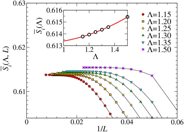
Next, we examine the and dependence of the total spin at impurity site defined in Eq. (42). In order to show more explicitly the and dependence, here we shall denote as when it is calculated using the logarithmic discretization scheme. We find in Fig. 17 that for a given is well converged when is sufficiently large. Note here that we set in Fig. 17. However, the extrapolated value of to , i.e.,
| (78) |
implying that is also taken with a finite and fixed ratio of , exhibits slight but visible dependence. As shown in the inset of Fig. 17, we find that is almost linearly dependent on when is close to 1, and the difference between with and the extrapolated value to , i.e.,
| (79) |
is quite small . We thus conclude that with can represent the value in the thermodynamic limit and the corresponding error is as small as . We should note here that the practical NRG calculations are typically performed with [51].
Next, let us compare the results for the logarithmic discretization scheme and the constant discretization scheme. We indeed find in Fig. 18 that, irrespectively of the discretization schemes, all results converge into a unique value in the limit of within the error of . More precisely, the results in Fig. 18 for the logarithmic and constant discretization schemes should converge to with and , respectively. We also find in Fig. 18 that the ratio , which we set to be 1 in our calculations shown in the main text, dose not affect the converged value as long as and are sufficiently large. For the logarithmic discretization scheme, the difference for various is found to be as small as .

B.3 Phase boundary in the thermodynamic limit
Here, we examine the phase boundary in the thermodynamic limit by explicitly taking the limits of and for the static quantities, i.e., the local density per spin and the total spin at the impurity site, calculated using the logarithmic discretization scheme. In order to show explicitly the and dependence of these quantities, here we adopt the convention used in Eqs. (78) and (79). Similarly, we take the limit of for the local density per spin calculated for given and , i.e.,
| (80) |
and then take the limit of , i.e.,
| (81) |
to estimate the value in the thermodynamic limit. To obtain the well-converged and predictive values of and within the residual error of , is required as large as 180 for .
Typical results around the phase boundary are shown in Figs. 19 and 20. We find in Figs. 19 and 20 that and exhibit the abrupt changes exactly at the same , i.e., , for each , although itself depends clearly on . The phase boundary in the thermodynamic limit is thus obtained by extrapolating to , i.e.,
| (82) |
As shown in the inset of Fig. 20, we find that for and , which is in excellent agreement with – estimated from the results for and in the main text (Figs. 3 and 5). We should also note that is very close to – for . Therefore, we conclude that the typical error of the phase boundary obtained in Figs. 3 and 5 is as small as .


B.4 Convergence behavior of dynamical quantities
Finally, we discuss the convergence of the dynamical quantities and for a given broadening factor . In order to make an accurate comparison, here we consider the noninteracting limit. In this limit, the spin excitation spectrum at the impurity site is given as
| (83) |
where is the impurity site component of the th eigenstate of in Eq. (II.2) with its eigenvalue . The charge excitation spectrum at the impurity site is expressed with the same form as in Eq. (83) except for the additional factor 4, i.e., , in the non-interacting limit. Therefore, we only consider below.
As shown in Fig. 21, we find that for smaller exhibits oscillating behavior when the constant discretization scheme is used. This is simply understood because the broadening factor is smaller than the level spacing of when is small. Therefore, the absence of such oscillating behavior for large enough is a hallmark of the convergence for a given . Indeed, we find in Fig. 21 that for is well converged, as compared with that for , and the estimated error is as small as .

We also notice in the insets of Fig. 21 that the similar oscillating behavior appears in the high-energy regions when the logarithmic discretization scheme is employed. This oscillating behavior is absent in the constant discretization scheme when the same is used. This is simply because, in the logarithmic discretization scheme, the energy mesh size is determined by and becomes wider in the higher-energy regions than in the lower-energy regions. In contrast, in the constant discretization scheme, the energy mesh size is constant for all energy regions and becomes smaller with increasing .

Aside from the slow convergence problem in the high energy regions, there is a more serious technical issue for the logarithmic discretization scheme. In the dynamical DMRG calculation for, e.g., the spin excitation spectrum at the impurity site, we have to construct the reduced density matrix of a mixed state composed of the ground state and the two excited states,
| (84) |
and
| (85) |
for each . Therefore, as compared with the ground state calculation, the convergence of the dynamical calculation is slower with respect to the number of the reduced density matrix eigenstates kept in the DMRG calculation. This is an additional source of numerical errors and depends sensitively on the discretization schemes.
Since
| (86) |
and
| (87) |
we can infer for each the errors in the two excited states and by evaluating
| (88) |
and
| (89) |
in the non-interacting limit, where is known exactly in Eq. (83) and when the particle-hole symmetry is preserved.
Figure 22 shows the results of and for the constant and logarithmic discretization schemes with keeping the same number of the reduced density matrix eigenstates and the same tolerance for the optimization of and [34]. As shown in Fig. 22, we find that both and for the logarithmic discretization scheme are larger than those for the constant discretization scheme. These results clearly show that the convergence of the excited states in the logarithmic discretization scheme is slow and thus a larger is required to reach the same convergence as in the constant discretization scheme, implying that the logarithmic discretization scheme demands more computational cost. Therefore, we employ the constant discretization scheme to calculate the full excitation spectra.
References
- [1] K. M. McCreary, A. G. Swartz, W. Han, J. Fabian, and R. K. Kawakami, Phys. Rev. Lett. 109, 186604 (2012).
- [2] R. R. Nair, M. Sepioni, I.-L. Tsai, O. Lehtinen, J. Keinonen, A. V. Krasheninnikov, T. Thomson, A. K. Geim, and I. V. Grigorieva, Nat. Phys. 8, 199 (2012).
- [3] A. H. C. Neto, F. Guinea, N. M. R. Peres, K. S. Novoselov, and A. K. Geim, Rev. Mod. Phys. 81, 109 (2009).
- [4] L. Fritz and M. Vojta, Rep. Prog. Phys. 76, 032501 (2013).
- [5] M. Vojta and L. Fritz, Phys. Rev. B 70, 094502 (2004).
- [6] L. Fritz and M. Vojta, Phys. Rev. B 70, 214427 (2004).
- [7] C. Gonzalez-Buxton and K. Ingersent, Phys. Rev. B 57, 14254 (1998).
- [8] R. Bulla, T. Pruschke, and C. Hewson, J. Phys.: Cond. Mat. 9, 10463 (1997).
- [9] R. Bulla, M. T. Glossop, D. E. Logan, and T. Pruschke, J. Phys.: Cond. Mat. 12, 4899 (2000).
- [10] K. Ingersent and Q. Si, Phys. Rev. Lett. 89, 076403 (2002).
- [11] T. Kanao, H. Matsuura, and M. Ogata, J. Phys. Soc. Jpn. 81, 063709 (2012).
- [12] H. Li and F. D. M. Haldane, Phys. Rev. Lett. 101, 010504 (2008).
- [13] L. Fidkowski, Phys. Rev. Lett. 104, 130502 (2010).
- [14] F. Pollmann, A. M. Turner, E. Berg, and M. Oshikawa, Phys. Rev. B 81, 064439 (2010).
- [15] T. Yoshida, R. Peters, S. Fujimoto, and N. Kawakami, Phys. Rev. Lett. 112, 196404 (2014).
- [16] S. Ejima, F. Lange, and H. Fehske, Phys. Rev. Lett. 113, 020401 (2014).
- [17] I. Affleck, Acta Phys. Pol. B 26, 1869 (1995).
- [18] A. Bayat, H. Johannesson, S. Bose, and P. Sodano, Nat. Comm. 5, 3784 (2014).
- [19] M. Vojta, Phil. Mag. 86, 1807 (2006).
- [20] S. R. White, Phys. Rev. Lett. 69, 2863 (1992).
- [21] S. R. White, Phys. Rev. B 48, 10345 (1993).
- [22] A. Chandran, V. Khemani, and S. L. Sondhi, Phys. Rev. Lett. 113, 060501 (2014).
- [23] K. G. Wilson, Rev. Mod. Phys. 47, 773 (1975).
- [24] R. Bulla, T. A. Costi, and T. Pruschke, Rev. Mod. Phys. 80, 395 (2008).
- [25] G. Lehmann, P. Rennert, M. Taut, and H. Wonn, Phys. Status Solidi 37, K27 (1970); G. Lehmann and M. Taut, ibid. 54, 469 (1972).
- [26] O. Jepsen and O. K. Andersen, Solid State Comm. 9 1763 (1971).
- [27] J. K. Cullum and R. A. Willoughby, Lanczos Algorithms for Large Symmetric Eigenvalue Computations (Birkhäuser, Boston, 1985).
- [28] D. J. García, K. Hallberg, and M. J. Rozenberg, Phys. Rev. Lett. 93, 246403 (2004).
- [29] R. Peters, Phys. Rev. B 84, 075139 (2011).
- [30] T. Shirakawa and S. Yunoki, Phys. Rev. B 90, 195109 (2014).
- [31] C. A. Büsser, G. B. Martins, and A. E. Feiguin, Phys. Rev. B 88, 245113 (2013).
- [32] A. Allerdt, C. A. Büsser, G. B. Martins, and A. E. Feiguin, Phys. Rev. B 91, 085101 (2015).
- [33] See, e.g.,A. C. Hewson, The Kondo Problem to Heavy Fermions (Cambridge University Press, New York, 1997).
- [34] E. Jeckelmann, Phys. Rev. B 66, 045114 (2002).
- [35] To be more precise, these three lowest entanglement levels are still quasi degenerate at as and . When we increase slightly to , we find that and . Further fine tuning of is required to reach at the exact three fold degenerate point, corresponding to the VF point at the phase boundary.
- [36] When is even and is finite, and are entangled, where and with represents the component of total spin ( in the left block excluding the impurity site. Therefore, the ground state is represented approximately as . We can now easily show that the lowest for is singlet.
- [37] In the ASC phase for , we find that the lowest entanglement level is non degenerate for both even and odd . This is because the total number of electrons in the left block is for even and for odd.
- [38] Z. Y. Meng, T. C. Lang, S. Wessel, F. F. Assaad, and A. Muramatsu, Nature 464, 847–851 (2010).
- [39] S. Sorella, Y. Otsuka, and S. Yunoki, Sci. Rep. 2, 992 (2012).
- [40] F. F. Assaad and I. F. Herbut, Phys. Rev. X 3, 031010 (2013).
- [41] F. Parisen Toldin, M. Hohenadler, F. F. Assaad, and I. F. Herbut, Phys. Rev. B 91, 165108 (2015).
- [42] Y. Otsuka, S. Yunoki, and S. Sorella, Phys. Rev. X 6, 011029 (2016).
- [43] W. Han, R. K. Kawakami, M. Gmitra, and J. Fabian, Nat. Nanotechnology 9, 794 (2014).
- [44] A. H. Castro Neto and F. Guinea, Phys. Rev. Lett. 103, 026804 (2009).
- [45] M. J. Schmidt and D. Loss, Phys. Rev. B 81, 165439 (2010).
- [46] C. Weeks, J. Hu, J. Alicea, M. Franz, and R. Wu, Phys. Rev. X 1, 021001 (2011).
- [47] J. Zhou, Q. F. Liang, and J. M. Dong, Carbon 48, 1405 (2010).
- [48] J. Balakrishnan, G. K. W. Koon, M. Jaiswal, A. H. Castro Neto, and B. Özyilmaz, Nat. Physics 9, 284 (2013).
- [49] D. Marchenko, A. Varykhalov, M. R. Scholz, G. Bihlmayer, E. I. Rashba, A. Rybkin, A. M. Shikin, and O. Rader, Nat. Comm. 3, 1232 (2012).
- [50] D. Mastrogiuseppe, A. Wong, K. Ingersent, S. E. Ulloa, and N. Sandler, Phys. Rev. B 90, 035426 (2014).
- [51] Ž. Osolin and R. Žitko, Phys. Rev. B 87, 245135 (2013).