Event excitation for event-driven control and optimization of multi-agent systems

The modeling and analysis of dynamic systems has historically been founded on the time-driven paradigm provided by a theoretical framework based on differential (or difference) equations: we postulate the existence of an underlying “clock” and with every “clock tick” a state update is performed which synchronizes all components of the system. As systems have become increasingly networked, wireless, and distributed, the universal value of this paradigm has come to question, since it may not be feasible to guarantee the synchronization of all components of a distributed system, nor is it efficient to trigger actions with every time step when such actions may be unnecessary. The event-driven paradigm offers an alternative to the modeling, control, communication, and optimization of dynamic systems. The main idea in event-driven methods is that actions affecting the system state need not be taken at each clock tick. Instead, one can identify appropriate events that trigger control actions. This approach includes the traditional time-driven view if a clock-tick is considered a system “event”. Defining the right events is a crucial modeling step and has to be carried out with a good understanding of the system dynamics.

The importance of event-driven behavior in dynamic systems was recognized in the development of Discrete Event Systems (DES) and later Hybrid Systems (HS) [1]. More recently there have been significant advances in applying event-driven methods (also referred to as “event-based” and “event-triggered”) to classical feedback control systems; e.g., see [2], [3], [4], as well as [5] and [6] and references therein. Event-driven approaches are also attractive in receding horizon control, where it is computationally inefficient to re-evaluate an optimal control value over small time increments as opposed to event occurrences defining appropriate planning horizons for the controller (e.g., see [7]). In distributed networked systems, event-driven mechanisms have the advantage of significantly reducing communication among networked components which cooperate to optimize a given objective. Maintaining such cooperation normally requires frequent communication among them; it was shown in [8] that we can limit ourselves to event-driven communication and still achieve optimization objectives while drastically reducing communication costs (hence, prolonging the lifetime of a wireless network), even when delays are present (as long as they are bounded).

Clearly, the premise of these methods is that the events involved are observable so as to “excite” the underlying event-driven controller. However, it is not always obvious that these events actually take place under every feasible control: it is possible that under some control no such events are excited, in which case the controller may be useless. In such cases, one can resort to artificial “timeout events” so as to eventually take actions, but this is obviously inefficient. Moreover, in event-driven optimization mechanisms this problem results in very slow convergence to an optimum or in an algorithm failing to generate any improvement in the decision variables being updated.

In this work, we address this issue of event excitation in the context of multi-agent systems. In this case, the events required are often defined by an agent “visiting” a region or a single point in a mission space $S\subset\mathbb{R}^{2}$. Clearly, it is possible that such events never occur for a large number of feasible agent trajectories. This is a serious problem in trajectory planning and optimization tasks which are common in multi-agent systems seeking to optimize different objectives associated with these tasks, including coverage, persistent monitoring or formation control [9], [10], [11, 12, 13, 14, 15, 16]. At the heart of this problem is the fact that objective functions for such tasks rely on a non-zero reward (or cost) metric associated with a subset $S^{+}\subset S$ of points, while all other points in $S$ have a reward (or cost) which is zero since they are not “points of interest” in the mission space. We propose a novel metric which allows all points in $S$ to acquire generally non-zero reward (or cost), thus ensuring that all events are ultimately excited. This leads to a new method allowing us to apply event-based control and optimization to a large class of multi-agent problems. We will illustrate the use of this method by considering a general trajectory optimization problem in which Infinitesimal Perturbation Analysis (IPA) [1] is used as an event-driven gradient estimation method to seek optimal trajectories for a class of multi-agent problems where the agents must cooperatively visit a set of target points to collect associated rewards (e.g., to collect data that are buffered at these points.) This defines a family within the class of Traveling Salesman Problems (TSPs) [17] for which most solutions are based on techniques typically seeking a shortest path in the underlying graph. These methods have several drawbacks: $(i)$ they are generally combinatorially complex, $(ii)$ they treat agents as particles (hence, not accounting for limitations in motion dynamics which should not, for instance, allow an agent to form a trajectory consisting of straight lines), and $(iii)$ they become computationally infeasible as on-line methods in the presence of stochastic effects such as random target rewards or failing agents. As an alternative we seek solutions in terms of parameterized agent trajectories which can be adjusted on line as a result of random effects and which are scalable, hence computationally efficient, especially in problems with large numbers of targets and/or agents. This approach was successfully used in [18], [19].

In section II we present the general framework for multi-agent problems and address the event excitation issue. In section III we overview the event-driven IPA methodology and how it is applied to a general hybrid system optimization problem. In section IV we introduce a data collection problem as an application of the general framework introduced in section II and will show simulation results of applying the new methodology to this example in section V.

Multi-agent systems are commonly modeled as hybrid systems with time-driven dynamics describing the motion of the agents or the evolution of physical processes in a given environment, while event-driven behavior characterizes events that may occur randomly (e.g., an agent failure) or in accordance to control policies (e.g., an agent stopping to sense the environment or to change directions). In some cases, the solution of a multi-agent dynamic optimization problem is reduced to a policy that is naturally parametric. As such, a multi-agent system can be studied with parameterized controllers aiming to meet certain specifications or to optimize a given performance metric. Moreover, in cases where such a dynamic optimization problem cannot be shown to be reduced to a parametric policy, using such a policy is still near-optimal or at least offers an alternative.

In order to build a general framework for multi-agent optimization problems, assuming $S$ as the mission space, we introduce the function $R(w):S\rightarrow\mathbb{R}$ as a “property” of point $w\in S$. For instance, $R(w)$ could be a weight that gives relative importance to one point in $S$ compared to another. Setting $R(w)>0$ for only a finite number of points implies that we limit ourselves to a finite set of points of interest while the rest of $S$ has no significant value.

Assuming $F$ to be the set of all feasible agent states, We define $P(w,s):S\times F\rightarrow\mathbb{R}$ to capture the cost/reward resulting from how agents with state $s\in F$ interact with $w\in S$. For instance, in coverage problems if an “event” occurs at $w$, then $P(w,s)$ is the probability of agents jointly detecting such events based on the relative distance of each agent from $w$.

In general settings, the objective is to find the best state vector $s_{1},\cdots,s_{N}$ so that $N$ agents achieve a maximal reward (minimal cost) from interacting with the mission space $S$:

$$\min_{s\in F}J=\int_{S}P(w,s)R(w)dw$$

(1)

This static problem can be extended to a dynamic version where the agents determine optimal trajectories $s_{i}(t),$ $t\in[0,T]$, rather than static states:

$$\min_{u(t)\in U}J=\int_{0}^{T}\int_{S}P(w,\mathbf{s}(u(t)))R(w,t)dwdt$$

(2)

subject to motion dynamics:

$$\dot{s}_{j}(t)=f_{j}(s_{j},u_{j},t),~j=1,\cdots,N$$

(3)

In Fig. 1, such a dynamic multi agent system is illustrated.

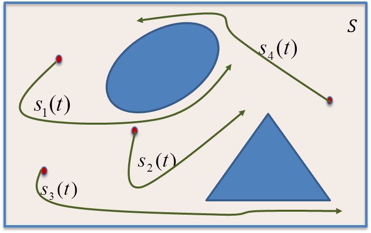
As an example, consensus problems are just a special case of (1). Suppose that we consider a finite set of points $w\in S$ which coincide with the agents states $s_{1},...,s_{N}$ (which are not necessarily their locations). Then we can set $P(w,s)=\|s_{i}-s_{j}\|^{2}$ and, therefore, replace the integral in (1) by a sum. In this case, $R(w)=R_{i}$ is just the weight that an agent carries in the consensus algorithm. An optimum occurs when $\|s_{i}-s_{j}\|^{2}=0$ for all $i,j$, i.e., all agents “agree” and consensus is reached. This is a special case because of the simplicity in $P(w,s)$ making the problem convex so that a global optimum can be achieved, in contrast to most problems we are interested in.

As for the formulation in (2), consider a trajectory planning problem where $N$ mobile agents are tasked to visit $M$ stationary targets in the mission space $S$. Target behavior is described through state variables $x_{i}(t)$ which may model reward functions, the amount of data present at $i$, or other problem-dependent target properties. More formally, let $(\Omega,\mathcal{F},\mathcal{P})$ be an appropriately defined probability space and $\omega\in\Omega$ a realization of the system where target dynamics are subject to random effects:

$$\dot{x}_{i}(t)=g_{i}(x_{i}(t),\omega)$$

(4)

$g_{i}(\cdot)$ is as such that $x_{i}(t)$ is monotonically increasing by $t$ and it resets to zero each time a target is completely emptied by an agent. In the context of (2), we assume the $M$ targets are located at points $w_{i},~i=1,\cdots,M$ and define

$$R(w,t)=\left\{\begin{array}[c]{ll}R(x_{i}(t),w)&\mbox{if }w\in C(w_{i})\\ 0&\mbox{otherwise}\end{array}\right.$$

(5)

to be the value of point $w$, where $C(w_{i})$ is a compact 2-manifold in $\mathbb{R}^{2}$ containing $w_{i}$ which can be considered to be a region defined by the sensing range of that target relative to agents (e.g., a disk centered at $w_{i}$). Note that $R(w,t)$ is also a random variable defined on the same probability space above. Given that only points $w\in C(w_{i})$ have value for the agents, there is an infinite number of points $w\notin C(w_{i})$ such that $R(w,t)=0$ provided the following condition holds:

Condition 1: If $\exists i~\mbox{such that}~w\in C(w_{i})$ then $w\notin C(w_{j})$ holds $\forall j\neq i$.

This condition is to ensure that two targets do not share any point $w$ in their respective sensing ranges. Also it ensures that the set $\{C(w_{i})~|~i=1:\cdots,M\}$ does not create a compact partitioning of the mission space and there exist points $w$ which do not belong to any of the $C(w_{i})$.

Viewed as a stochastic hybrid system, we may define different modes depending on the states of agents or targets and events that cause transitions between these modes. Relative to a target $i$, any agent has at least two modes: being at a point $w\in C(w_{i})$, i.e., visiting this target or not visiting it. Within each mode, agent $j$’s dynamics, dictated by (3), and target $i$’s dynamics in (4) may vary. Accordingly, there are at least two types of events in such a system: $(i)$ $\delta_{ij}^{0}$ events occur when agent $j$ initiates a visit at target $i$, and $(ii)$ $\delta_{ij}^{+}$ events occur when agent $j$ ends a visit at target $i$. Additional event types may be included depending on the specifics of a problem, e.g., mode switches in the target dynamics or agents encountering obstacles.

An example is shown in Fig. 2, where target sensing ranges are shown with green circles and agent trajectories are shown in dashed lines starting at a base shown by a red triangle. In the blue trajectory, agent $1$ moves along the trajectory that passes through points $A\rightarrow B\rightarrow C\rightarrow D$. It is easy to see that when passing through points $A$ and $C$ we have $\delta_{i1}^{0}$ and $\delta_{i^{\prime}1}^{0}$ events, while passing through $B$ and $D$ we have $\delta_{i1}^{+}$ and $\delta_{i^{\prime}1}^{+}$ events. The red trajectory is an example where none of the events is excited. Suppose we consider an on-line trajectory adjustment process in which the agent improves its trajectory based on its performance measured through (5). In this case, $R(w,t)=0$ over all $t$, as long as the agent keeps using the red trajectory, i.e., no event ever occurs. Therefore, if an event-driven approach is used to control the trajectory adjustment process, no action is ever triggered and the approach is ineffective. In contrast, in the blue trajectory the controller can extract useful information from every observed event; such information (e.g., a gradient of $J$ with respect to controllable parameters as described in the next section) can be used to adjust the current trajectory so as to improve the objective function $J$ in (1) or (2).

Therefore, if we are to build an optimization framework for this class of stochastic hybrid systems to allow the application of event-driven methods by calculating a performance measure gradient, then a fundamental property required is the occurrence of at least some events in a sample realization. In particular, the IPA method [20] is based on a single sample realization of the system over which events are observed along with their occurrence times and associated system states. Suppose that the trajectories can be controlled through a set of parameters forming a vector $\theta$. Then, IPA provides an unbiased estimate of the gradient of a performance metric $J(\theta)$ with respect to $\theta$. This gradient is then used to improve the trajectory and ultimately seek an optimal one when appropriate conditions hold.

As in the example of Fig. 2, it is possible to encounter trajectory realizations where no events occur in the system. In the above example, this can easily happen if the trajectory does not pass through any target. The existence of such undesirable trajectories is the direct consequence of Condition 1. This lack of event excitation results in event-based controllers being unsuitable.

New Metric: In order to overcome this issue we propose a new definition for $R(w,t)$ in (5) as follows:

$$R(w,t)=\sum_{i=1}^{M}h_{i}(x_{i}(t),d_{i}(w))$$

(6)

where $w\in S$, $h_{i}(\cdot)$ is a function of the target’s state $x_{i}(t)$ and $d_{i}(w)=\|w_{i}-w\|$. Note that, if $h_{i}(\cdot)$ is properly defined, (6) yields $R(w,t)>0$ at all points.

While the exact form of $h_{i}(\cdot)$ depends on the problem, we impose the condition that $h_{i}(\cdot)$ is monotonically decreasing in $d_{i}(w)$. We can think of $h_{i}(\cdot)$ as a value function associated with point $w_{i}$. Using the definition of $R(w,t)$, this value is spread out over all points $w\in S$ rather than being concentrated at the single point $w_{i}$. This creates a continuous potential field for the agents leading to a non-zero gradient of the performance measure even when the trajectories do not excite any events. This non-zero gradient will then induce trajectory adjustments that naturally bring them toward ones with observable events.

Finally, recalling the definition in (2), we also define:

$$P(w,s)=\sum_{j=1}^{N}\|s_{j}(t)-w\|^{2}$$

(7)

the total quadratic travel cost for agents to visit point $w$.

In Section IV, we will show how to apply $R(w,t)$ and $P(w,s)$ defined as above in order to determine optimal agent trajectories for a class of multi-agent problems of the form (2). First, however, we review in the next section the event-driven IPA calculus which allows us to estimate performance gradients with respect to controllable parameters.

Let us fix a particular value of the parameter $\bm{\theta}\in\Theta$ and study a resulting sample path of a general SHS. Over such a sample path, let $\tau_{k}(\bm{\theta})$, $k=1,2,\cdots$ denote the occurrence times of the discrete events in increasing order, and define $\tau_{0}(\bm{\theta})=0$ for convenience. We will use the notation $\tau_{k}$ instead of $\tau_{k}(\bm{\theta})$ when no confusion arises. The continuous state is also generally a function of $\bm{\theta}$, as well as of $t$, and is thus denoted by $x(\bm{\theta},t)$. Over an interval $[\tau_{k}(\bm{\theta}),\tau_{k+1}(\bm{\theta}))$, the system is at some mode during which the time-driven state satisfies $\dot{x}=f_{k}(x,\bm{\theta},t)$, in which $x$ is any of the continuous state variables of the system and $\dot{x}$ denotes $\frac{\partial x}{\partial t}$ . Note that we suppress the dependence of $f_{k}$ on the inputs $u\in U$ and $d\in D$ and stress instead its dependence on the parameter $\bm{\theta}$ which may generally affect either $u$ or $d$ or both. The purpose of perturbation analysis is to study how changes in $\bm{\theta}$ influence the state $x(\bm{\theta},t)$ and the event times $\tau_{k}(\bm{\theta})$ and, ultimately, how they influence interesting performance metrics that are generally expressed in terms of these variables.

An event occurring at time $\tau_{k+1}(\bm{\theta})$ triggers a change in the mode of the system, which may also result in new dynamics represented by $f_{k+1}$. The event times ${\tau_{k}(\bm{\theta})}$ play an important role in defining the interactions between the time-driven and event-driven dynamics of the system.

Following the framework in [20], consider a general performance function $J$ of the control parameter $\bm{\theta}$:

$$J(\bm{\theta};x(\bm{\theta},0),T)=E[L(\bm{\theta};x(\bm{\theta},0),T)]$$

(8)

where $L(\bm{\theta};x(\bm{\theta},0),T)$ is a sample function of interest evaluated in the interval $[0,T]$ with initial conditions $x(\theta,0)$. For simplicity, we write $J(\bm{\theta})$ and $L(\bm{\theta})$. Suppose that there are $K$ events, with occurrence times generally dependent on $\bm{\theta}$, during the time interval $[0,T]$ and define $\tau_{0}=0$ and $\tau_{N+1}=T$. Let $L_{k}:\mathbb{R}^{n}\times\Theta\times\mathbb{R}^{+}\rightarrow\mathbb{R}$ be a function and define $L(\bm{\theta})$ by

$$L(\bm{\theta})=\sum_{k=0}^{K}\int_{\tau_{k}}^{\tau_{k+1}}L_{k}(x,\theta,t)dt$$

(9)

where we reiterate that $x=x(\bm{\theta},t)$ is a function of $\bm{\theta}$ and $t$. We also point out that the restriction of the definition of $J(\bm{\theta})$ to a finite horizon $T$ which is independent of $\bm{\theta}$ is made merely for the sake of simplicity. Returning to the stochastic setting, the ultimate goal of the iterative process shown is to maximize $E_{\omega}[L(\bm{\theta},\omega)]$, where we use $\omega$ to emphasize dependence on a sample path $\omega$ of a SHS (clearly, this is reduced to $L(\bm{\theta})$ in the deterministic case). Achieving such optimality is possible under standard ergodicity conditions imposed on the underlying stochastic processes, as well as the assumption that a single global optimum exists; otherwise, the gradient-based approach is simply continuously attempting to improve the observed performance $L(\bm{\theta},\omega)$. Thus, we are interested in estimating the gradient

$$\frac{dJ(\bm{\theta})}{d\bm{\theta}}=\frac{dE_{\omega}[L(\bm{\theta},\omega)]}{d\bm{\theta}}$$

(10)

by evaluating $\frac{dL(\bm{\theta},\omega)}{d\theta}$ based on directly observed data. We obtain $\bm{\theta}^{\ast}$ by optimizing $J(\bm{\theta})$ through an iterative scheme of the form

$$\bm{\theta}_{n+1}=\bm{\theta}_{n}-\eta_{n}H_{n}(\bm{\theta}_{n};x(\bm{\theta},0),T,\omega_{n}),~n=0,1,\cdots$$

(11)

where ${\eta_{n}}$ is a step size sequence and $H_{n}(\bm{\theta}_{n};x(\bm{\theta},0),T,\omega_{n})$ is the estimate of $\frac{dJ(\bm{\theta})}{d\bm{\theta}}$ at $\bm{\theta}=\bm{\theta}_{n}$. In using IPA, $H_{n}(\bm{\theta}_{n};x(\bm{\theta},0),T,\omega_{n})$ is the sample derivative $\frac{dL(\bm{\theta},\omega)}{d\bm{\theta}}$ , which is an unbiased estimate of $\frac{dJ(\bm{\theta})}{d\bm{\theta}}$ if the condition (dropping the symbol $\omega$ for simplicity)

$$E\big[\frac{dL(\bm{\theta})}{d\bm{\theta}}\big]=\frac{dE[L(\bm{\theta})]}{d\bm{\theta}}=\frac{dJ(\bm{\theta})}{d\bm{\theta}}$$

(12)

is satisfied, which turns out to be the case under mild technical conditions. The conditions under which algorithms of the form (11) converge are well-known (e.g., see [21]). Moreover, in addition to being unbiased, it can be shown that such gradient estimates are independent of the probability laws of the stochastic processes involved and require minimal information from the observed sample path. The process through which IPA evaluates $\frac{dL(\bm{\theta})}{d\bm{\theta}}$ is based on analyzing how changes in $\bm{\theta}$ influence the state $x(\bm{\theta},t)$ and the event times $\tau_{k}(\bm{\theta})$. In turn, this provides information on how $L(\bm{\theta})$ is affected, because it is generally expressed in terms of these variables. Given $\bm{\theta}=[\theta_{1},...,\theta_{l}]^{T}$, we use the Jacobian matrix notation:

$$x^{\prime}(\bm{\theta},t)=\frac{\partial x(\bm{\theta},t)}{\partial\bm{\theta}},~{\tau_{k}}^{\prime}=\frac{\partial\tau_{k}(\bm{\theta})}{\partial\bm{\theta}},k=1,\cdots,K$$

(13)

for all state and event time derivatives. For simplicity of notation, we omit $\theta$ from the arguments of the functions above unless it is essential to stress this dependence. It is shown in [20] that $x^{\prime}(t)$ satisfies:

$$\frac{dx^{\prime}(t)}{dt}=\frac{\partial f_{k}(t)}{\partial x}x^{\prime}(t)+\frac{\partial f_{k}(t)}{\partial\bm{\theta}}$$

(14)

for $t\in[\tau_{k}(\theta),\tau_{k+1|}(\theta))$ with boundary condition

$$x^{\prime}(\tau_{k}^{+})=x^{\prime}(\tau_{k}^{-})+[f_{k-1}(\tau_{k}^{-})-f_{k}(\tau_{k}^{+})]\tau_{k}^{\prime}$$

(15)

for $k=0,\cdots,K$. We note that whereas $x(t)$ is often continuous in $t$, $x^{\prime}(t)$ may be discontinuous in $t$ at the event times $\tau_{k}$; hence, the left and right limits above are generally different. If $x(t)$ is not continuous in $t$ at $t=\tau_{k}(\bm{\theta})$, the value of $x(\tau_{k}^{+})$ is determined by the reset function $r(q,q^{\prime},x,\nu,\delta)$ and

$$x^{\prime}(\tau_{k}^{+})=\frac{dr(q,q^{\prime},x,\nu,\delta)}{d\bm{\theta}}$$

(16)

Furthermore, once the initial condition $x^{\prime}(\tau_{k}^{+})$ is given, the linearized state trajectory ${x^{\prime}(t)}$ can be computed in the interval $t\in[\tau_{k}(\bm{\theta}),\tau_{k+1}(\bm{\theta}))$ by solving (14) to obtain

$$x^{\prime}(t)=e^{\int_{\tau_{k}}^{t}\frac{\partial f_{k}(u)}{\partial x}du}\Big[\int_{\tau_{k}}^{t}\frac{\partial f_{k}(v)}{\partial\bm{\theta}}e^{-\int_{\tau_{k}}^{t}\frac{\partial f_{k}(u)}{\partial x}du}dv+\xi_{k}\Big]$$

(17)

with the constant $\xi_{k}$ determined from $x^{\prime}(\tau_{k}^{+})$. In order to complete the evaluation of $x^{\prime}(\tau_{k}^{+})$ we need to also determine $\tau_{k}^{\prime}$. If the event at $\tau_{k}(\theta)$ is exogenous $\tau_{k}^{\prime}=0$ and if the event at $\tau_{k}(\theta)$ is endogenous:

$$\tau_{k}^{\prime}=-\Big[\frac{\partial g_{k}}{\partial x}f_{k}(\tau_{k}^{-})\Big]\big(\frac{\partial g_{k}}{\partial\bm{\theta}}+\frac{\partial g_{k}}{\partial x}x^{\prime}(\tau_{k}^{-})\big)$$

(18)

where $g_{k}(x,\bm{\theta})=0$ and it is defined as long as $\frac{\partial g_{k}}{\partial x}f_{k}(\tau_{k}^{+})\neq 0$ (details may be found in [20].)

The derivative evaluation process involves using the IPA calculus in order to evaluate the IPA derivative $\frac{dL}{d\bm{\theta}}$. This is accomplished by taking derivatives in (9) with respect to $\bm{\theta}$:

$$\frac{dL(\bm{\theta})}{d\bm{\theta}}=\sum_{k=0}^{K}\frac{d}{d\bm{\theta}}\int_{\tau_{k}}^{\tau_{k+1}}L_{k}(x,\bm{\theta},t)dt$$

(19)

Applying the Leibnitz rule, we obtain, for every $k=0,\cdots,K,$

$$\begin{split}\frac{d}{d\bm{\theta}}&\int_{\tau_{k}}^{\tau_{k+1}}L_{k}(x,\bm{\theta},t)dt\\ &=\int_{\tau_{k}}^{\tau_{k+1}}\Big[\frac{\partial L_{k}(x,\bm{\theta},t)}{\partial x}x^{\prime}(t)+\frac{\partial L_{k}(x,\bm{\theta},t)}{\partial\bm{\theta}}\Big]dt\\ &+L_{k}(x(\tau_{k+1}),\bm{\theta},\tau_{k+1})\tau_{k+1}^{\prime}-L_{k}(x(\tau_{k}),\bm{\theta},\tau_{k})\tau_{k}^{\prime}\end{split}$$

(20)

In summary the three equations (15), (17) and (18) form the basis of the IPA calculus and allow us to calculate the final derivative in (20). In the next section IPA is applied to a data collection problem in a multi-agent system.

We consider a class of multi-agent problems where the agents must cooperatively visit a set of target points to collect associated rewards (e.g., to collect data that are buffered at these points.). The mission space is $S\subset\mathbb{R}^{2}$. This class of problems falls within the general formulation introduced in (2). The state of the system is the position of agent $j$ time $t$, $s_{j}(t)=[s_{j}^{x}(t),s_{j}^{y}(t)]$ and the state of the target $i$, $x_{i}(t)$. The agent’s dynamics (3) follow a single integrator:

$$\dot{s}_{j}^{x}(t)=u_{j}(t)\cos\theta_{j}(t),\quad\ \ \dot{s}_{j}^{y}(t)=u_{j}(t)\sin\theta_{j}(t)$$

(21)

where $u_{j}(t)$ is the scalar speed of the agent (normalized so that $0\leq u_{j}(t)\leq 1$) and $\theta_{j}(t)$ is the angle relative to the positive direction, $0\leq\theta_{j}(t)<2\pi$. Thus, we assume that each agent controls its speed and heading.

We assume the state of the target $x_{i}(t)$ represents the amount of data that is currently available at target $i$ (this can be modified to different state interpretations). The dynamics of $x_{i}(t)$ in (4) for this problem are:

$\dot{x}_{i}(t)=\left\{\begin{array}[]{ll}0\qquad\mbox{if }x_{i}(t)=0\mbox{ and }\sigma_{i}(t)\leq\mu_{ij}p(s_{j}(t),w_{i})&\\ \sigma_{i}(t)-\mu_{ij}p(s_{j}(t),w_{i})\qquad\qquad\qquad\mbox{otherwise}&\end{array}\right.$

(22)

i.e., we model the data at the target as satisfying simple flow dynamics with an exogenous (generally stochastic) inflow $\sigma_{i}(t)$ and a controllable rate with which an agent empties the data queue given by $\mu_{ij}p(s_{j}(t),w_{i})$. For brevity we set $p(s_{j}(t),w_{i})=p_{ij}(t)$ which is the normalized data collection rate from target $i$ by agent $j$ and $\mu_{ij}$ is a nominal rate corresponding to target $i$ and agent $j$.

Assuming $M$ targets are located at $w_{i}\in S,$ $i=1,\dots,M,$ and have a finite range of $r_{i}$, then agent $j$ can collect data from $w_{i}$ only if $d_{ij}(t)=\|w_{i}-s_{j}(t)\|\leq r_{i}$. We then assume that: $(\mathbf{A1})$ $p_{ij}(t)\in[0,1]$ is monotonically non-increasing in the value of $d_{ij}(t)=\|w_{i}-s_{j}(t)\|$, and $(\mathbf{A2})$ it satisfies $p_{ij}(t)=0$ if $d_{ij}(t)>r_{i}$. Thus, $p_{ij}(t)$ can model communication power constraints which depend on the distance between a data source and an agent equipped with a receiver (similar to the model used in [22]) or sensing range constraints if an agent collects data using on-board sensors. For simplicity, we will also assume that: $(\mathbf{A3})$ $p_{ij}(t)$ is continuous in $d_{ij}(t)$ and $(\mathbf{A4})$ only one agent at a time is connected to a target $i$ even if there are other agents $l$ with $p_{il}(t)>0$; this is not the only possible model, but we adopt it based on the premise that simultaneous downloading of packets from a common source creates problems of proper data reconstruction. This means that $j$ in (22) is the index of the agent that is connected to target $i$ at time $t$.

The dynamics of $x_{i}(t)$ in (22) results in two new event types added to what was defined earlier, $(i)$ $\xi_{i}^{0}$ events occur when $x_{i}(t)$ reaches zero, and $(ii)$ $\xi_{i}^{+}$ events occur when $x_{i}(t)$ leaves zero.

The performance measure is the total content of data left at targets at the end of a finite mission time $T$. Thus, we define $J_{1}(t)$ to be the following (recalling that $\{\sigma_{i}(t)\}$ are random processes):

$$J_{1}(t)=\sum\limits_{i=1}^{M}\alpha_{i}E[x_{i}(t)]$$

(23)

where $\alpha_{i}$ is a weight factor for target $i$. We can now formulate a stochastic optimization problem $\mathbf{P1}$ where the control variables are the agent speeds and headings denoted by the vectors $\mathbf{u}(t)=[u_{1}(t),\dots,u_{N}(t)]$ and ${\theta}(t)=[\theta_{1}(t),\dots,\theta_{N}(t)]$ respectively (omitting their dependence on the full system state at $t$).

$$\mathbf{P1:}\qquad\qquad\quad\min\limits_{\mathbf{u(t),\theta(t)}}J(T)=\frac{1}{T}\int_{0}^{T}J_{1}(t)dt\quad\quad$$

(24)

where $0\leq u_{j}(t)\leq 1$, $0\leq\theta_{j}(t)<2\pi$, and $T$ is a given finite mission time. This problem can be readily placed into the general framework (2). In particular, the right hand side of (24) is:

$$\begin{split}&\frac{1}{T}E\left[\int_{0}^{T}\sum_{i}\int_{C(w_{i})}\frac{\alpha_{i}}{\pi r_{i}^{2}}x_{i}(t)dwdt\right]\\ =&\frac{1}{T}E\left[\int_{0}^{T}\int_{S}\sum_{i}\frac{\alpha_{i}\bm{1}\{w\in C(w_{i})\}}{\pi r_{i}^{2}}x_{i}(t)dwdt\right]\end{split}$$

(25)

This is now in the form of the general framework in (2) with

$$R(w,t)=\sum_{i}\frac{\alpha_{i}\bm{1}\{w\in C(w_{i})\}}{\pi r_{i}^{2}}x_{i}(t)$$

(26)

and

$$P(s_{j}(t),w)=1$$

(27)

Recalling the definition in (5), only points within the sensing range of each target have non-zero values, while all other point value are zero, which is the case in (26) above. In addition, (27) simply shows that there is no meaningful dynamic interaction between an agent and the environment.

Problem $\mathbf{P1}$ is a finite time optimal control problem. In order to solve this, following previous work in [19] we proceed with a standard Hamiltonian analysis leading to a Two Point Boundary Value Problem (TPBVP) [23]. We omit this, since the details are the same as the analysis in [19]. The main result of the Hamiltonian analysis is that the optimal speed is always the maximum value, i.e.,

$$u_{j}^{\ast}(t)=1$$

(28)

Hence, we only need to calculate the optimal $\theta_{j}(t)$. This TPBVP is computationally expensive and easily becomes intractable when problem size grows. The ultimate solution of the TPBVP is a set of agent trajectories that can be put in a parametric form defined by a parameter vector $\bm{\theta}$ and then optimized over $\bm{\theta}$. If the parametric trajectory family is broad enough, we can recover the true optimal trajectories; otherwise, we can approximate them within some acceptable accuracy. Moreover, adopting a parametric family of trajectories and seeking an optimal one within it has additional benefits: it allows trajectories to be periodic, often a desirable property, and it allows one to restrict solutions to trajectories with desired features that the true optimal may not have, e.g., smoothness properties to achieve physically feasible agent motion.

Parameterizing the trajectories and using gradient based optimization methods, in light of the discussions from the previous sections, enables us to make use of Infinitesimal Perturbation Analysis (IPA) [20] to carry out the trajectory optimization process. We represent each agent’s trajectory through general parametric equations

$$\begin{array}[c]{ll}s_{j}^{x}(t)=f_{x}(\bm{\theta}_{j},\rho_{j}(t)),\text{ \ }\quad s_{j}^{y}(t)=f_{y}(\bm{\theta}_{j},\rho_{j}(t))&\end{array}$$

(29)

where the function $\rho_{j}(t)$ controls the position of the agent on its trajectory at time $t$ and $\bm{\theta}_{j}$ is a vector of parameters controlling the shape and location of the trajectory. Let $\bm{\theta}=[\bm{\theta}_{1},\dots,\bm{\theta}_{N}]$. We now revisit problem $\mathbf{P1}$ in (24):

$$\begin{split}\min\limits_{\bm{\theta}\in\Theta}J(\bm{\theta},T)=\frac{1}{T}\int_{0}^{T}J_{1}(\bm{\theta},t)dt\end{split}$$

(30)

and will bring in the equations that were introduced in the previous section in order to calculate an estimate of $\frac{dJ(\bm{\theta})}{d\bm{\theta}}$ as in (10). For this problem due to the continuity of $x_{i}(t)$ the last two terms in (20) vanish. From (23) we have:

$$\begin{split}\frac{d}{d\bm{\theta}}\int_{\tau_{k}}^{\tau_{k+1}}\sum_{i=1}^{M}\alpha_{i}x_{i}(\bm{\theta},t)dt=\int_{\tau_{k}}^{\tau_{k+1}}\sum_{i=1}^{M}\alpha_{i}x_{i}^{\prime}(\bm{\theta},t)dt\end{split}$$

(31)

In summary, the evaluation of (31) requires the state derivatives $x_{i}^{\prime}(t)$ explicitly and $s_{j}^{\prime}(t)$ implicitly, (dropping the dependence on $\bm{\theta}$ for brevity). The latter are easily obtained for any specific choice of $f$ and $g$ in (29). The former require a rather laborious use of (15),(17),(18) which, reduces to a simple set of state derivative dynamics as shown next.

Proposition 1. After an event occurrence at $t=\tau_{k}$, the state derivatives $x_{i}^{\prime}(\tau_{k}^{+})$ with respect to the controllable parameter $\bm{\theta}$ satisfy the following:

$$x_{i}^{\prime}(\tau_{k}^{+})=\left\{\begin{array}[c]{ll}0&\text{if }e(\tau_{k})=\xi_{i}^{0}\\ x_{i}^{\prime}(\tau_{k}^{-})-\mu_{il}(t)p_{il}(\tau_{k}){\tau_{k}^{{}^{\prime}}}&\text{if }e(\tau_{k})=\delta_{ij}^{+}\\ x_{i}^{\prime}(\tau_{k}^{-})&\text{otherwise}\end{array}\right.$$

where $l\neq j$ with $p_{il}(\tau_{k})>0$ if such $l$ exists and ${\tau_{k}^{{}^{\prime}}=}\frac{\partial d_{ij}(s_{j})}{\partial s_{j}}s^{\prime}_{j}\left(\frac{\partial d_{ij}(s_{j})}{\partial s_{j}}\dot{s}_{j}(\tau_{k})\right)^{-1}$.

We provide some simulation results based on an elliptical parametric description for the trajectories in (29). The elliptical trajectory formulation is:

$$\begin{array}[]{ll}s_{j}^{x}(t)=&A_{j}+a_{j}\cos\rho_{j}(t)\cos\phi_{j}-b_{j}\sin\rho_{j}(t)\sin\phi_{j}\\ s_{j}^{y}(t)=&B_{j}+a_{j}\cos\rho_{j}(t)\sin\phi_{j}+b_{j}\sin\rho_{j}(t)\cos\phi_{j}\end{array}$$

(45)

Here, $\theta_{j}=[A_{j},B_{j},a_{j},b_{j},\phi_{j}]$ where $A_{j},B_{j}$ are the coordinates of the center, $a_{j}$ and $b_{j}$ are the major and minor axis respectively while $\phi_{j}\in[0,\pi)$ is the ellipse orientation which is defined as the angle between the $x$ axis and the major axis of the ellipse. The time-dependent parameter $\rho_{j}(t)$ is the eccentric anomaly of the ellipse. Since an agent is moving with constant speed of 1 on this trajectory, based on (28), we have $\dot{s}_{j}^{x}(t)^{2}+\dot{s}_{j}^{y}(t)^{2}=1$, which gives

$\begin{split}\dot{\rho}_{j}(t)=\Big[&\Big(a\sin\rho_{j}(t)\cos\phi_{j}+b_{j}\cos\rho_{j}(t)\sin\phi_{j}\Big)^{2}\\ &+\Big(a\sin\rho_{j}(t)\sin\phi_{j}-b_{j}\cos\rho_{j}(t)\cos\phi_{j}\Big)^{2}\Big]^{-\frac{1}{2}}\end{split}$

(46)

The first case we consider is a problem with one agent and seven targets located on a circle, as shown in Fig. 4. We consider a deterministic case with $\sigma_{i}(t)=0.5$ for all $i$. The other problem parameters are $T=50$, $\mu_{ij}=100$, $r_{i}=0.2$ and $\alpha_{i}=1$. A target’s sensing range is denoted with solid black circles with the target location at the center. The blue polygon indicates the convex hull produced by the targets. The direction of motion on a trajectory is shown with the small arrow. Starting with an initial trajectory shown in light blue, the on-line trajectory optimization process converges to the trajectory passing through all targets in an efficient manner (shown in dark solid blue). In contrast, starting with this trajectory - which does not pass through any targets - problem $\mathbf{P1}$ does not converge and the initial trajectory remains unchanged. At the final trajectory, $J_{1}^{\ast}=0.0859$ and $J^{\ast}=0.2128$. Using the obvious shortest path solution, the actual optimal value for $J_{1}$ is $0.0739$ that results from moving on the edges of the convex hull (which allows for shorter agent travel times).

References

- [1] C. G. Cassandras and S. Lafortune, Introduction to Discrete Event Systems. Secaucus, NJ, USA: Springer-Verlag New York, Inc., 2006.
- [2] W. Heemels, J. Sandee, and P. P. J. van den Bosch, “Analysis of event-driven controllers for linear systems,” International journal of control, vol. 81, no. 4, pp. 571–590, 2008.
- [3] A. Anta and P. Tabuada, “To sample or not to sample: Self-triggered control for nonlinear systems,” Automatic Control, IEEE Trans. on, vol. 55, pp. 2030–2042, Sept 2010.
- [4] S. Trimpe and R. D’Andrea, “Event-based state estimation with variance-based triggering,” Automatic Control, IEEE Trans. on, vol. 59, no. 12, pp. 3266–3281, 2014.
- [5] M. Miskowicz, Event-Based Control and Signal Processing. CRC Press, 2015.
- [6] C. G. Cassandras, “The event-driven paradigm for control, communication and optimization,” Journal of Control and Decision, vol. 1, no. 1, pp. 3–17, 2014.
- [7] Y. Khazaeni and C. G. Cassandras, “A new event-driven cooperative receding horizon controller for multi-agent systems in uncertain environments,” In Proceedings of IEEE 53rd Annual Conference on Decision and Control, pp. 2770–2775, Dec 2014.
- [8] M. Zhong and C. G. Cassandras, “Asynchronous distributed optimization with event-driven communication,” Automatic Control, IEEE Trans. on, vol. 55, no. 12, pp. 2735–2750, 2010.
- [9] M. Schwager, D. Rus, and J.-J. Slotine, “Decentralized, adaptive coverage control for networked robots,” The International Journal of Robotics Research, vol. 28, no. 3, pp. 357–375, 2009.
- [10] C. G. Cassandras, X. Lin, and X. Ding, “An optimal control approach to the multi-agent persistent monitoring problem,” IEEE Trans. on Aut. Cont., vol. 58, pp. 947–961, April 2013.
- [11] M. Cao, A. Morse, C. Yu, B. Anderson, and S. Dasgupta, “Maintaining a directed, triangular formation of mobile autonomous agents,” Communications in Information and Systems, vol. 11, no. 1, p. 1, 2011.
- [12] K.-K. Oh and H.-S. Ahn, “Formation control and network localization via orientation alignment,” IEEE Trans. on Automatic Control, vol. 59, pp. 540–545, Feb 2014.
- [13] H. Yamaguchi and T. Arai, “Distributed and autonomous control method for generating shape of multiple mobile robot group,” in Proc. of the IEEE International Conf. on Intelligent Robots and Systems, vol. 2, pp. 800–807 vol.2, Sep 1994.
- [14] J. Desai, V. Kumar, and J. Ostrowski, “Control of changes in formation for a team of mobile robots,” in Proc. of the IEEE International Conf. on Robotics and Automation, vol. 2, pp. 1556–1561, 1999.
- [15] M. Ji and M. B. Egerstedt, “Distributed coordination control of multi-agent systems while preserving connectedness.,” IEEE Trans. on Robotics, vol. 23, no. 4, pp. 693–703, 2007.
- [16] J. Wang and M. Xin, “Integrated optimal formation control of multiple unmanned aerial vehicles,” IEEE Trans. on Control Systems Technology, vol. 21, pp. 1731–1744, Sept 2013.
- [17] D. L. Applegate, R. E. Bixby, V. Chvatal, and W. J. Cook, The traveling salesman problem: a computational study. Princeton University Press, 2011.
- [18] X. Lin and C. G. Cassandras, “An optimal control approach to the multi-agent persistent monitoring problem in two-dimensional spaces,” IEEE Trans. on Automatic Control, vol. 60, pp. 1659–1664, June 2015.
- [19] Y. Khazaeni and C. G. Cassandras, “An optimal control approach for the data harvesting problem,” in 54th IEEE Conf. on Decision and Cont., pp. 5136–5141, 2015.
- [20] C. G. Cassandras, Y. Wardi, C. G. Panayiotou, and C. Yao, “Perturbation analysis and optimization of stochastic hybrid systems,” European Journal of Cont., vol. 16, no. 6, pp. 642 – 661, 2010.
- [21] H. Kushner and G. Yin, Stochastic Approximation and Recursive Algorithms and Applications. Springer, 2003.
- [22] J. L. Ny, M. a. Dahleh, E. Feron, and E. Frazzoli, “Continuous path planning for a data harvesting mobile server,” Proc. of the IEEE Conf. on Decision and Cont., pp. 1489–1494, 2008.
- [23] A. E. Bryson and Y. C. Ho, Applied optimal control: optimization, estimation and control. CRC Press, 1975.
- [24] Y. Khazaeni and C. G. Cassandras, “An optimal control approach for the data harvesting problem,” arXiv:1503.06133.