跳到论文正文
W Papers独立论文阅读器 arXiv:1604.00645 论文正文 计算阅读时间 · 0%
引用这篇论文根据当前论文元数据生成,正式投稿前建议核对。


License: arXiv.org perpetual non-exclusive license
arXiv:1604.00645v2 [cs.IT] 08 Apr 2016

Analysis and Optimization of Caching and Multicasting in Large-Scale Cache-Enabled Heterogeneous Wireless Networks

Ying Cui ††thanks: Y. Cui and D. Jiang are with the Department of Electronic Engineering, Shanghai Jiao Tong University, China.    MIEEE    Dongdong Jiang    StMIEEE
Abstract

Heterogeneous wireless networks (HetNets) provide a powerful approach to meet the dramatic mobile traffic growth, but also impose a significant challenge on backhaul. Caching and multicasting at macro and pico base stations (BSs) are two promising methods to support massive content delivery and reduce backhaul load in HetNets. In this paper, we jointly consider caching and multicasting in a large-scale cache-enabled HetNet with backhaul constraints. We propose a hybrid caching design consisting of identical caching in the macro-tier and random caching in the pico-tier, and a corresponding multicasting design. By carefully handling different types of interferers and adopting appropriate approximations, we derive tractable expressions for the successful transmission probability in the general region as well as the high signal-to-noise ratio (SNR) and user density region, utilizing tools from stochastic geometry. Then, we consider the successful transmission probability maximization by optimizing the design parameters, which is a very challenging mixed discrete-continuous optimization problem. By using optimization techniques and exploring the structural properties, we obtain a near optimal solution with superior performance and manageable complexity. This solution achieves better performance in the general region than any asymptotically optimal solution, under a mild condition. The analysis and optimization results provide valuable design insights for practical cache-enabled HetNets.

Index Terms: 
Cache, multicast, backhaul, stochastic geometry, optimization, heterogenous wireless network

I Introduction

The rapid proliferation of smart mobile devices has triggered an unprecedented growth of the global mobile data traffic. HetNets have been proposed as an effective way to meet the dramatic traffic growth by deploying short range small-BSs together with traditional macro-BSs, to provide better time or frequency reuse[1]. However, this approach imposes a significant challenge of providing expensive high-speed backhaul links for connecting all the small-BSs to the core network[2].

Caching at small-BSs is a promising approach to alleviate the backhaul capacity requirement in HetNets[3, 4, 5]. Many existing works have focused on optimal cache placement at small-BSs, which is of critical importance in cache-enabled HetNets. For example, in [6] and [7], the authors consider the optimal content placement at small-BSs to minimize the expected downloading time for files in a single macro-cell with multiple small-cells. File requests which cannot be satisfied locally at a small-BS are served by the macro-BS. The optimization problems in [6] and [7] are NP-hard, and low-complexity solutions are proposed. In [8], the authors propose a caching design based on file splitting and MDS encoding in a single macro-cell with multiple small-cells. File requests which cannot be satisfied locally at a small-BS are served by the macro-BS, and backhaul rate analysis and optimization are considered. Note that the focuses of [6, 7, 8] are on performance optimization of caching design.

In [9, 10, 11], the authors consider caching the most popular files at each small-BS in large-scale cache-enabled small-cell networks or HetNets, with backhaul constraints. The service rates of uncached files are limited by the backhaul capacity. In [12], the authors propose a partion-based combined caching design in a large-scale cluster-centric small-cell network, without considering backhaul constraints. In [13], the authors consider two caching designs, i.e., caching the most popular files and random caching of a uniform distribution, at small-BSs in a large-scale cache-enabled HetNet, without backhaul constraints. File requests which cannot be satisfied at a small-BS are served by macro-BSs. In [14], the authors consider random caching of a uniform distribution in a large-scale cache-enabled small-cell network, without backhaul constraints, assuming that content requests follow a uniform distribution. Note that the focuses of [9, 10, 11, 12, 13, 14] are on performance analysis of caching designs.

On the other hand, enabling multicast service at BSs in HetNets is an efficient way to deliver popular contents to multiple requesters simultaneously, by effectively utilizing the broadcast nature of the wireless medium[15]. In [16] and [17], the authors consider a single macro-cell with multiple small-cells with backhaul costs. Specifically, in [16], the optimization of caching and multicasting, which is NP-hard, is considered, and a simplified solution with approximation guarantee is proposed. In [17], the optimization of dynamic multicast scheduling for a given content placement, which is a dynamic programming problem, is considered, and a low-complexity optimal numerical solution is obtained.

The network models considered in [6, 7, 8, 16, 17] do not capture the stochastic natures of channel fading and geographic locations of BSs and users. The network models considered in [9, 10, 11, 12, 13, 14] are more realistic and can reflect the stochastic natures of signal and interference. However, the simple identical caching design considered in [9, 10, 11, 13] does not provide spatial file diversity; the combined caching design in [12] does not reflect the popularity differences of files in each of the three categories; and the random caching design of a uniform distribution in [13, 14] cannot make use of popularity information. Hence, the caching designs in [9, 10, 11, 12, 13, 14] may not lead to good network performance. On the other hand, [18, 19, 20, 21] consider analysis and optimization of caching in large-scale cache-enabled single-tier networks. Specifically, [18] considers random caching at BSs, and analyze and optimize the hit probability. Reference [19] considers random caching with contents being stored at each BS in an i.i.d. manner, and analyzes the minimum offloading loss. In [20], the authors study the expected costs of obtaining a complete content under random uncoded caching and coded caching strategies, which are designed only for different pieces of a single content. In [21], the authors consider analysis and optimization of joint caching and multicasting. However, the proposed caching and multicasting designs in [18, 19, 20, 21] may not be applicable to HetNets with backhaul constraints. In summary, to facilitate designs of practical cache-enabled HetNets for massive content dissemination, further studies are required to understand the following key questions.

∙\bullet How do physical layer and content-related parameters fundamentally affect performance of cache-enabled HetNets?

∙\bullet How can caching and multicasting jointly and optimally assist massive content dissemination in cache-enabled HetNets?

In this paper, we consider the analysis and optimization of joint caching and multicasting to improve the efficiency of massive content dissemination in a large-scale cache-enabled HetNet with backhaul constraints. Our main contributions are summarized below.

∙\bullet First, we propose a hybrid caching design with certain design parameters, consisting of identical caching in the macro-tier and random caching in the pico-tier, which can provide spatial file diversity. We propose a corresponding multicasting design for efficient content dissemination by exploiting broadcast nature of the wireless medium.

∙\bullet Then, by carefully handling different types of interferers and adopting appropriate approximations, we derive tractable expressions for the successful transmission probability in the general region and the asymptotic region, utilizing tools from stochastic geometry. These expressions reveal the impacts of physical layer and content-related parameters on the successful transmission probability.

∙\bullet Next, we consider the successful transmission probability maximization by optimizing the design parameters, which is a very challenging mixed discrete-continuous optimization problem. We propose a two-step optimization framework to obtain a near optimal solution with superior performance and manageable complexity. Specifically, we first characterize the structural properties of the asymptotically optimal solutions. Then, based on these properties, we obtain the near optimal solution, which achieves better performance in the general region than any asymptotically optimal solution, under a mild condition.

∙\bullet Finally, by numerical simulations, we show that the near optimal solution achieves a significant gain in successful transmission probability over some baseline schemes.

II Network Model

We consider a two-tier HetNet where a macro-cell tier is overlaid with a pico-cell tier, as shown in Fig. 1. The locations of the macro-BSs and the pico-BSs are spatially distributed as two independent homogeneous Poisson point processes (PPPs) Φ1\Phi_{1} and Φ2\Phi_{2} with densities λ1\lambda_{1} and λ2\lambda_{2}, respectively, where λ1<λ2\lambda_{1}<\lambda_{2}. The locations of the users are also distributed as an independent homogeneous PPP Φu\Phi_{u} with density λu\lambda_{u}. We refer to the macro-cell tier and the pico-cell tier as the 11st tier and the 22nd tier, respectively. Consider the downlink scenario. Each BS in the jjth tier has one transmit antenna with transmission power PjP_{j} (j=1,2j=1,2), where P1>P2P_{1}>P_{2}. Each user has one receive antenna. All BSs are operating on the same frequency band of total bandwidth WW (Hz). Consider a discrete-time system with time being slotted and study one slot of the network. We consider both large-scale fading and small-scale fading. Due to large-scale fading, a transmitted signal from the jjth tier with distance DD is attenuated by a factor 1Dαj\frac{1}{D^{\alpha_{j}}}, where αj>2\alpha_{j}>2 is the path loss exponent of the jjth tier. For small-scale fading, we assume Rayleigh fading channels[22, 23].

Let 𝒩≜{1,2,⋯,N}\mathcal{N}\triangleq\{1,2,\cdots,N\} denote the set of NN files (e.g., data objects or chucks of data objects) in the HetNet. For ease of illustration, assume that all files have the same size.11 1 Files of different sizes can be divided into chunks of the same length. Thus, the results in this paper can be extended to the case of different file sizes. Each file is of certain popularity, which is assumed to be identical among all users. Each user randomly requests one file, which is file n∈𝒩n\in\mathcal{N} with probability an∈(0,1)a_{n}\in(0,1), where ∑n∈𝒩an=1\sum_{n\in\mathcal{N}}a_{n}=1. Thus, the file popularity distribution is given by 𝐚≜(an)n∈𝒩\mathbf{a}\triangleq(a_{n})_{n\in\mathcal{N}}, which is assumed to be known apriori. In addition, without loss of generality (w.l.o.g.), assume a1>a2>…>aNa_{1}>a_{2}>\ldots>a_{N}.

The HetNet consists of cache-enabled macro-BSs and pico-BSs. Each BS in the jjth tier is equipped with a cache of size Kjc<NK_{j}^{c}<N to store different files. Assume K1c+K2c≤NK_{1}^{c}+K_{2}^{c}\leq N. Each macro-BS is connected to the core network via a wireline backhaul link of transmission capacity K1b<NK_{1}^{b}<N (files/slot), i.e., each macro-BS can retrieve at most K1bK_{1}^{b} different files from the core network in each slot.22 2 Note that storing or retrieving more than one copies of the same file at one BS is redundant and will waste storage or backhaul resources. Note that K1cK_{1}^{c}, K2cK_{2}^{c} and K1bK_{1}^{b} reflect the storage and backhaul resources in the cache-enabled HetNet.

Refer to caption
Fig. 1: Network model. The 1st tier corresponds to a Voronoi tessellation (cf. black dashed line segments), determined by the locations of all the macro-BSs. Each file n∈ℱ2cn\in\mathcal{F}_{2}^{c} corresponds to a Voronoi tessellation (cf. solid line segments in the same color as the file), determined by the locations of all the pico-BSs storing this file.

III Joint Caching and Multicasting

We are interested in the case where the storage and backhaul resources are limited, and may not be able to satisfy all file requests. In this section, we propose a joint caching and multicasting design with certain design parameters, which can provide high spatial file diversity and ensure efficient content dissemination.

III-A Hybrid Caching

To provide high spatial file diversity, we propose a hybrid caching design consisting of identical caching in the 1st tier and random caching in the 2nd tier, as illustrated in Fig. 1. Let ℱjc⊆𝒩\mathcal{F}_{j}^{c}\subseteq\mathcal{N} denote the set of Fjc≜|ℱjc|F_{j}^{c}\triangleq|\mathcal{F}_{j}^{c}| files cached in the jjth tier. Specifically, our hybrid caching design satisfies the following requirements: (i) non-overlapping caching across tiers: each file is stored in at most one tier; (ii) identical caching in the 1st tier: each macro-BS stores the same set ℱ1c\mathcal{F}_{1}^{c} of K1cK_{1}^{c} (different) files; and (iii) random caching in the 2nd tier: each pico-BS randomly stores K2cK_{2}^{c} different files out of all files in ℱ2c\mathcal{F}_{2}^{c}, forming a subset of ℱ2c\mathcal{F}_{2}^{c}. Thus, we have the following constraint:

ℱ1c,ℱ2c⊆𝒩,ℱ1c∩ℱ2c=∅,F1c=K1c,F2c≥K2c.\displaystyle\mathcal{F}_{1}^{c},\mathcal{F}_{2}^{c}\subseteq\mathcal{N},\ \mathcal{F}_{1}^{c}\cap\mathcal{F}_{2}^{c}=\emptyset,\ F_{1}^{c}=K_{1}^{c},\ F_{2}^{c}\geq K_{2}^{c}. (1)

To further illustrate the random caching in the 2nd tier, we first introduce some notations. We say every K2cK_{2}^{c} different files in ℱ2c\mathcal{F}_{2}^{c} form a combination. Thus, there are I≜(F2cK2c)I\triangleq\binom{F_{2}^{c}}{K_{2}^{c}} different combinations in total. Let ℐ≜{1,2,⋯,I}\mathcal{I}\triangleq\{1,2,\cdots,I\} denote the set of II combinations. Combination i∈ℐi\in\mathcal{I} can be characterized by an F2cF_{2}^{c}-dimensional vector 𝐱i≜(xi,n)n∈ℱ2c\mathbf{x}_{i}\triangleq(x_{i,n})_{n\in\mathcal{F}_{2}^{c}}, where xi,n=1x_{i,n}=1 indicates that file n∈ℱ2cn\in\mathcal{F}_{2}^{c} is included in combination ii and xi,n=0x_{i,n}=0 otherwise. Note that there are K2cK_{2}^{c} 1’s in each 𝐱i\mathbf{x}_{i}. Denote 𝒩i≜{n∈ℱ2c:xi,n=1}⊆ℱ2c\mathcal{N}_{i}\triangleq\{n\in\mathcal{F}_{2}^{c}:x_{i,n}=1\}\subseteq\mathcal{F}_{2}^{c} as the set of K2cK_{2}^{c} files contained in combination ii. Each pico-BS stores one combination at random, which is combination i∈ℐi\in\mathcal{I} with probability pip_{i} satisfying:33 3 In this paper, to understand the natures of joint caching and multicasting in cache-enabled HetNets, we shall first pose the analysis and optimization on the basis of all the file combinations in ℐ\mathcal{I} (for the 2nd tier). Then, based on the insights obtained, we shall focus on reducing complexity while maintaining superior performance.

0≤pi≤1,i∈ℐ,\displaystyle 0\leq p_{i}\leq 1,\ i\in\mathcal{I}, (2)
∑i∈ℐpi=1.\displaystyle\sum_{i\in\mathcal{I}}p_{i}=1. (3)

Denote 𝐩≜(pi)i∈ℐ\mathbf{p}\triangleq(p_{i})_{i\in\mathcal{I}}. To facilitate the analysis in later sections, based on 𝐩\mathbf{p}, we also define the probability that file n∈ℱ2cn\in\mathcal{F}_{2}^{c} is stored at a pico-BS, i.e.,

Tn≜∑i∈ℐnpi,n∈ℱ2c,\displaystyle T_{n}\triangleq\sum_{i\in\mathcal{I}_{n}}p_{i},\ n\in\mathcal{F}_{2}^{c}, (4)

where ℐn≜{i∈ℐ:xi,n=1}\mathcal{I}_{n}\triangleq\{i\in\mathcal{I}:x_{i,n}=1\} denotes the set of In≜(F2c−1K2c−1)I_{n}\triangleq\binom{F_{2}^{c}-1}{K_{2}^{c}-1} combinations containing file n∈ℱ2cn\in\mathcal{F}_{2}^{c}. Denote 𝐓≜(Tn)n∈ℱ2c\mathbf{T}\triangleq(T_{n})_{n\in\mathcal{F}_{2}^{c}}. Note that 𝐩\mathbf{p} and 𝐓\mathbf{T} depend on ℱ2c\mathcal{F}_{2}^{c}. Thus, in this paper, we use 𝐩⁡(ℱ2c)\mathbf{p}(\mathcal{F}_{2}^{c}) and 𝐓⁡(ℱ2c)\mathbf{T}(\mathcal{F}_{2}^{c}) when emphasizing this relation. Therefore, the hybrid caching design in the cache-enabled HetNet is specified by the design parameters (ℱ1c,ℱ2c,𝐩)\left(\mathcal{F}_{1}^{c},\mathcal{F}_{2}^{c},\mathbf{p}\right).

To efficiently utilize backhaul links and ensure high spatial file diversity, we only retrieve files not stored in the cache-enabled HetNet via backhaul links. Let ℱ1b⊆𝒩\mathcal{F}_{1}^{b}\subseteq\mathcal{N} denote the set of F1b≜|ℱ1b|F_{1}^{b}\triangleq|\mathcal{F}_{1}^{b}| files which can be retrieved by each macro-BS from the core network. Thus, we have the following constraint:

ℱ1b=𝒩∖(ℱ1c∪ℱ2c).\displaystyle\mathcal{F}_{1}^{b}=\mathcal{N}\setminus(\mathcal{F}_{1}^{c}\cup\mathcal{F}_{2}^{c}). (5)

Therefore, the file distribution in the cache-enabled HetNet is fully specified by the hybrid caching design (ℱ1c,ℱ2c,𝐩)\left(\mathcal{F}_{1}^{c},\mathcal{F}_{2}^{c},\mathbf{p}\right).

III-B Multicasting

In this part, we propose a multicasting design associated with the hybrid caching design (ℱ1c,ℱ2c,𝐩)\left(\mathcal{F}_{1}^{c},\mathcal{F}_{2}^{c},\mathbf{p}\right). First, we introduce the user association under the proposed hybrid caching design. In the cache-enabled HetNet, a user accesses to a tier based on its desired file. Specifically, each user requesting file n∈ℱ1c∪ℱ1bn\in\mathcal{F}_{1}^{c}\cup\mathcal{F}_{1}^{b} is associated with the nearest macro-BS and is referred to as a macro-user. While, each user requesting file n∈ℱ2cn\in\mathcal{F}_{2}^{c} is associated with the nearest pico-BS storing a combination i∈ℐni\in\mathcal{I}_{n} (containing file nn) and is referred to as a pico-user. The associated BS of each user is called its serving BS, and offers the maximum long-term average receive power for its desired file[23]. Note that under the proposed hybrid caching design (ℱ1c,ℱ2c,𝐩)\left(\mathcal{F}_{1}^{c},\mathcal{F}_{2}^{c},\mathbf{p}\right), the serving BS of a macro-user is its nearest macro-BS, while the serving BS of a pico-user (affected by 𝐩\mathbf{p}) may not be its geographically nearest BS. We refer to this association mechanism as the content-centric association in the cached-enabled HetNet, which is different from the traditional connection-based association [23] in HetNets.

Now, we introduce file scheduling in the cache-enabled HetNet. Each BS will serve all the cached files requested by its associated users. Each macro-BS only serves at most K1bK_{1}^{b} uncached files requested by its associated users, due to the backhaul constraint for retrieving uncached files. In particular, if the users of a macro-BS request smaller than or equal to K1bK_{1}^{b} different uncached files, the macro-BS serves all of them; if the users of a macro-BS request greater than K1bK_{1}^{b} different uncached files, the macro-BS will randomly select K1bK_{1}^{b} different requested uncached files to serve, out of all the requested uncached files according to the uniform distribution.

We consider multicasting44 4 Note that in this paper, the multicast service happens once every slot, and hence no additional delay is introduced. in the cache-enabled HetNet for efficient content dissemination. Suppose a BS schedules to serve requests for kk different files. Then, it transmits each of the kk files at rate τ\tau (bit/second) and over 1k\frac{1}{k} of total bandwidth W using FDMA. All the users which request one of the kk files from this BS try to decode the file from the single multicast transmission of the file at the BS. Note that, by avoiding transmitting the same file multiple times to multiple users, this content-centric transmission (multicast) can improve the efficiency of the utilization of the wireless medium and reduce the load of the wireless links, compared to the traditional connection-based transmission (unicast).

From the above illustration, we can see that the proposed multicasting design is also affected by the proposed hybrid caching design (ℱ1c,ℱ2c,𝐩)\left(\mathcal{F}_{1}^{c},\mathcal{F}_{2}^{c},\mathbf{p}\right). Therefore, the design parameters (ℱ1c,ℱ2c,𝐩)\left(\mathcal{F}_{1}^{c},\mathcal{F}_{2}^{c},\mathbf{p}\right) affect the performance of the proposed joint caching and multicasting design.

IV Performance Metric

In this paper, w.l.o.g., we study the performance of the typical user denoted as u0u_{0}, which is located at the origin. We assume all BSs are active. Suppose u0u_{0} requests file nn. Let j0j_{0} denote the index of the tier to which u0u_{0} belongs, and let j¯0\overline{j}_{0} denote the other tier. Let ℓ0∈Φj0\ell_{0}\in\Phi_{j_{0}} denote the index of the serving BS of u0u_{0}. We denote Dj,ℓ,0D_{j,\ell,0} and hj,ℓ,0∼d𝒞​𝒩​(0,1)h_{j,\ell,0}\stackrel{{\scriptstyle d}}{{\sim}}\mathcal{CN}\left(0,1\right) as the distance and the small-scale channel between BS ℓ∈Φj\ell\in\Phi_{j} and u0u_{0}, respectively. We assume the complex additive white Gaussian noise of power N0N_{0} at u0u_{0}. When u0u_{0} requests file nn and file nn is transmitted by BS ℓ0\ell_{0}, the signal-to-interference plus noise ratio (SINR) of u0u_{0} is given by

SINRn,0=Dj0,ℓ0,0−αj0​|hj0,ℓ0,0|2∑ℓ∈Φj0\ℓ0Dj0,ℓ,0−αj0​|hj0,ℓ,0|2+∑ℓ∈Φj¯0Dj¯0,ℓ,0−αj¯0​|hj¯0,ℓ,0|2​Pj¯0Pj0+N0Pj0,n∈𝒩.\displaystyle{\rm SINR}_{n,0}=\frac{{D_{j_{0},\ell_{0},0}^{-\alpha_{j_{0}}}}\left|h_{j_{0},\ell_{0},0}\right|^{2}}{\sum_{\ell\in\Phi_{j_{0}}\backslash\ell_{0}}D_{j_{0},\ell,0}^{-\alpha_{j_{0}}}\left|h_{j_{0},\ell,0}\right|^{2}+\sum_{\ell\in\Phi_{\overline{j}_{0}}}D_{\overline{j}_{0},\ell,0}^{-\alpha_{\overline{j}_{0}}}\left|h_{\overline{j}_{0},\ell,0}\right|^{2}\frac{P_{\overline{j}_{0}}}{P_{j_{0}}}+\frac{N_{0}}{P_{j_{0}}}},\ n\in\mathcal{N}. (6)

When u0u_{0} requests file n∈ℱ1cn\in\mathcal{F}_{1}^{c} (n∈ℱ1bn\in\mathcal{F}_{1}^{b}), let K1,n,0c∈{1,⋯,K1c}K_{1,n,0}^{c}\in\{1,\cdots,K_{1}^{c}\} (K¯1,n,0c∈{0,⋯,K1c}\overline{K}_{1,n,0}^{c}\in\{0,\cdots,K_{1}^{c}\}) and K¯1,n,0b∈{0,⋯,F1b}\overline{K}_{1,n,0}^{b}\in\{0,\cdots,F_{1}^{b}\} (K1,n,0b∈{1,⋯,F1b}K_{1,n,0}^{b}\in\{1,\cdots,F_{1}^{b}\}) denote the numbers of different cached and uncached files requested by the users associated with BS ℓ0∈Φ1\ell_{0}\in\Phi_{1}, respectively. When u0u_{0} requests file n∈ℱ2cn\in\mathcal{F}_{2}^{c}, let K2,n,0c∈{1,⋯,K2c}K_{2,n,0}^{c}\in\{1,\cdots,K_{2}^{c}\} denote the number of different cached files requested by the users associated with BS ℓ0∈Φ2\ell_{0}\in\Phi_{2}. Note that K1,n,0c,K¯1,n,0b,K¯1,n,0c,K1,n,0b,K2,n,0cK_{1,n,0}^{c},\overline{K}_{1,n,0}^{b},\overline{K}_{1,n,0}^{c},K_{1,n,0}^{b},K_{2,n,0}^{c} are discrete random variables, the probability mass functions (p.m.f.s) of which depend on 𝐚\mathbf{a}, λu\lambda_{u} and the design parameters (ℱ1c,ℱ2c,𝐩)\left(\mathcal{F}_{1}^{c},\mathcal{F}_{2}^{c},\mathbf{p}\right). In addition, if n∈ℱ1c∪ℱ2cn\in\mathcal{F}_{1}^{c}\cup\mathcal{F}_{2}^{c}, BS ℓ0\ell_{0} will transmit file nn for sure; if n∈ℱ1bn\in\mathcal{F}_{1}^{b}, for given K1,n,0b=kb≥1K_{1,n,0}^{b}=k^{b}\geq 1, BS ℓ0\ell_{0} will transmit file nn with probability min⁡{kb,K1b}kb\frac{\min\{k^{b},K_{1}^{b}\}}{k^{b}}. Given that file nn is transmitted, it can be decoded correctly at u0u_{0} if the channel capacity between BS ℓ0\ell_{0} and u0u_{0} is greater than or equal to τ\tau. Requesters are mostly concerned with whether their desired files can be successfully received. Therefore, in this paper, we consider the successful transmission probability of a file requested by u0u_{0} as the network performance metric. By total probability theorem, the successful transmission probability under the proposed scheme is given by:

q⁡(ℱ1c,ℱ2c,𝐩)=q1​(ℱ1c,ℱ2c)+q2​(ℱ2c,𝐩),\displaystyle q(\mathcal{F}_{1}^{c},\mathcal{F}_{2}^{c},\mathbf{p})=q_{1}(\mathcal{F}_{1}^{c},\mathcal{F}_{2}^{c})+q_{2}(\mathcal{F}_{2}^{c},\mathbf{p}), (7)

where ℱ1b\mathcal{F}_{1}^{b} is given by (5), and q1​(ℱ1c,ℱ2c)q_{1}(\mathcal{F}_{1}^{c},\mathcal{F}_{2}^{c}) and q2​(ℱ2c,𝐩)q_{2}(\mathcal{F}_{2}^{c},\mathbf{p}) are given by (8) and (9), respectively. Note that in (8) and (9), each term multiplied by ana_{n} represents the successful transmission probability of file nn.

q1​(ℱ1c,ℱ2c)=\displaystyle q_{1}(\mathcal{F}_{1}^{c},\mathcal{F}_{2}^{c})= ∑n∈ℱ1canPr[WK1,n,0c+min⁡{K1b,K¯1,n,0b}log2(1+SINRn,0)≥τ]\displaystyle\sum_{n\in\mathcal{F}_{1}^{c}}a_{n}{\rm Pr}\left[\frac{W}{K_{1,n,0}^{c}+\min\{K_{1}^{b},\overline{K}_{1,n,0}^{b}\}}\log_{2}\left(1+{\rm SINR}_{n,0}\right)\geq\tau\right]
+∑n∈ℱ1banPr[WK¯1,n,0c+min⁡{K1b,K1,n,0b}log2(1+SINRn,0)≥τ,n is selected]\displaystyle+\sum_{n\in\mathcal{F}_{1}^{b}}a_{n}{\rm Pr}\left[\frac{W}{\overline{K}_{1,n,0}^{c}+\min\{K_{1}^{b},K_{1,n,0}^{b}\}}\log_{2}\left(1+{\rm SINR}_{n,0}\right)\geq\tau,\text{$n$ is selected}\right] (8)
q2​(ℱ2c,𝐩)=\displaystyle q_{2}(\mathcal{F}_{2}^{c},\mathbf{p})= ∑n∈ℱ2canPr[WK2,n,0clog2(1+SINRn,0)≥τ]\displaystyle\sum_{n\in\mathcal{F}_{2}^{c}}a_{n}{\rm Pr}\left[\frac{W}{K_{2,n,0}^{c}}\log_{2}\left(1+{\rm SINR}_{n,0}\right)\geq\tau\right] (9)


Later, we shall see that under the proposed caching and multicasting design for content-oriented services in the cache-enabled HetNet, the successful transmission probability is sufficiently different from the traditional rate coverage probability studied for connection-oriented services [23]. In particular, the successful transmission probability considered in this paper not only depends on the physical layer parameters, such as the macro and pico BS densities λ1\lambda_{1} and λ2\lambda_{2}, user density λu\lambda_{u}, path loss exponents α1\alpha_{1} and α2\alpha_{2}, bandwidth WW, backhaul capacity K1bK_{1}^{b} and transmit signal-to-noise ratios (SNRs) P1N0\frac{P_{1}}{N_{0}} and P2N0\frac{P_{2}}{N_{0}}, but also relies on the content-related parameters, such as the popularity distribution 𝐚\mathbf{a}, the cache sizes K1cK_{1}^{c} and K2cK_{2}^{c}, and the design parameters (ℱ1c,ℱ2c,𝐩⁡(ℱ2c))\left(\mathcal{F}_{1}^{c},\mathcal{F}_{2}^{c},\mathbf{p}(\mathcal{F}_{2}^{c})\right). While, the traditional rate coverage probability only depends on the physical layer parameters. In addition, the successful transmission probability depends on the physical layer parameters in a different way from the traditional rate coverage probability. For example, the content-centric association leads to different distributions of the locations of serving and interfering BSs; the multicasting transmission results in different file load distributions at each BS [23]; and the cache-enabled architecture makes content availability related to BS densities.

V Performance Analysis

In this section, we study the successful transmission probability q⁡(ℱ1c,ℱ2c,𝐩)q\left(\mathcal{F}_{1}^{c},\mathcal{F}_{2}^{c},\mathbf{p}\right) under the proposed caching and multicasting design for given design parameters (ℱ1c,ℱ2c,𝐩⁡(ℱ2c))\left(\mathcal{F}_{1}^{c},\mathcal{F}_{2}^{c},\mathbf{p}(\mathcal{F}_{2}^{c})\right). First, we analyze the successful transmission probability in the general region. Then, we analyze the asymptotic transmission probability in the high SNR and user density region.

V-A Performance Analysis in General Region

In this part, we would like to analyze the successful transmission probability in the general region, using tools from stochastic geometry. In general, file loads K1,n,0cK_{1,n,0}^{c}, K¯1,n,0b\overline{K}_{1,n,0}^{b}, K¯1,n,0c\overline{K}_{1,n,0}^{c}, K1,n,0bK_{1,n,0}^{b}, K2,n,0cK_{2,n,0}^{c} and SINR SINRn,0{\rm SINR}_{n,0} are correlated in a complex manner, as BSs with larger association regions have higher file load and lower SINR (due to larger user to BS distance) [24]. For the tractability of the analysis, as in [23] and [24], the dependence is ignored. Therefore, to obtain the successful transmission probability in (7), we analyze the distributions of K1,n,0cK_{1,n,0}^{c}, K¯1,n,0b\overline{K}_{1,n,0}^{b}, K¯1,n,0c\overline{K}_{1,n,0}^{c}, K1,n,0bK_{1,n,0}^{b}, K2,n,0cK_{2,n,0}^{c} and the distribution of SINRn,0{\rm SINR}_{n,0}, separately.

First, we calculate the p.m.f.s of K1,n,0cK_{1,n,0}^{c} and K¯1,n,0b\overline{K}_{1,n,0}^{b} for n∈ℱ1cn\in\mathcal{F}_{1}^{c} as well as the p.m.f.s of K¯1,n,0c\overline{K}_{1,n,0}^{c} and K1,n,0bK_{1,n,0}^{b} for n∈ℱ1bn\in\mathcal{F}_{1}^{b}. In calculating these p.m.f.s, we need the probability density function (p.d.f.) of the size of the Voronoi cell of ℓ0\ell_{0} w.r.t. file m∈ℱ1c∪ℱ1b∖{n}m\in\mathcal{F}_{1}^{c}\cup\mathcal{F}_{1}^{b}\setminus\{n\}. Note that this p.d.f. is equivalent to the p.d.f. of the size of the Voronoi cell to which a randomly chosen user belongs. Based on a tractable approximated form of this p.d.f. in [25], which is widely used in existing literature[24, 23], we obtain the p.m.f.s of K1,n,0cK_{1,n,0}^{c}, K¯1,n,0b\overline{K}_{1,n,0}^{b}, K¯1,n,0c\overline{K}_{1,n,0}^{c} and K1,n,0bK_{1,n,0}^{b}.

Lemma 1 (p.m.f.s of K1,n,0cK_{1,n,0}^{c} K¯1,n,0b\overline{K}_{1,n,0}^{b}, K¯1,n,0c\overline{K}_{1,n,0}^{c} and K1,n,0bK_{1,n,0}^{b})

The p.m.f.s of K1,n,0cK_{1,n,0}^{c} and K¯1,n,0b\overline{K}_{1,n,0}^{b} for n∈ℱ1cn\in\mathcal{F}_{1}^{c} and the p.m.f.s of K¯1,n,0c\overline{K}_{1,n,0}^{c} and K1,n,0bK_{1,n,0}^{b} for n∈ℱ1bn\in\mathcal{F}_{1}^{b} are given by

Pr[K1,n,0c=kc]=g(ℱ1,−nc,kc−1),kc=1,⋯,K1c,\displaystyle\Pr\left[K_{1,n,0}^{c}=k^{c}\right]=g(\mathcal{F}_{1,-n}^{c},k^{c}-1),\quad k^{c}=1,\cdots,K_{1}^{c}, (10)
Pr[K¯1,n,0b=kb]=g(ℱ1b,kb),kb=0,⋯,F1b,\displaystyle\Pr\left[\overline{K}_{1,n,0}^{b}=k^{b}\right]=g(\mathcal{F}_{1}^{b},k^{b}),\quad k^{b}=0,\cdots,F_{1}^{b}, (11)
Pr[K¯1,n,0c=kc]=g(ℱ1c,kc),kc=0,⋯,K1c,\displaystyle\Pr\left[\overline{K}_{1,n,0}^{c}=k^{c}\right]=g(\mathcal{F}_{1}^{c},k^{c}),\quad k^{c}=0,\cdots,K_{1}^{c}, (12)
Pr[K1,n,0b=kb]=g(ℱ1,−nb,kb−1),kb=1,⋯,F1b,\displaystyle\Pr\left[K_{1,n,0}^{b}=k^{b}\right]=g(\mathcal{F}_{1,-n}^{b},k^{b}-1),\quad k^{b}=1,\cdots,F_{1}^{b}, (13)

where g(ℱ,k)≜∑𝒳∈{𝒮⊆ℱ:|𝒮|=k}∏m∈𝒳(1−(1+am​λu3.5​λ1)−4.5)∏m∈ℱ∖𝒳(1+am​λu3.5​λ1)−4.5g(\mathcal{F},k)\triangleq\sum_{\mathcal{X}\in\left\{\mathcal{S}\subseteq\mathcal{F}:|\mathcal{S}|=k\right\}}\prod_{m\in\mathcal{X}}\left(1-\left(1+\frac{a_{m}\lambda_{u}}{3.5\lambda_{1}}\right)^{-4.5}\right)\prod_{m\in{\mathcal{F}\setminus\mathcal{X}}}\left(1+\frac{a_{m}\lambda_{u}}{3.5\lambda_{1}}\right)^{-4.5},   ℱ1,−nc≜ℱ1c∖{n}\mathcal{F}_{1,-n}^{c}\triangleq\mathcal{F}_{1}^{c}\setminus\{n\} and ℱ1,−nb≜ℱ1b∖{n}\mathcal{F}_{1,-n}^{b}\triangleq\mathcal{F}_{1}^{b}\setminus\{n\}.

Proof:

Please refer to Appendix A. ∎

Next, we obtain the p.m.f. of K2,n,0cK_{2,n,0}^{c} for n∈ℱ2cn\in\mathcal{F}_{2}^{c}. In calculating the p.m.f. of K2,n,0cK_{2,n,0}^{c}, we need the p.d.f. of the size of the Voronoi cell of ℓ0\ell_{0} w.r.t. file m∈𝒩i∖{n}m\in\mathcal{N}_{i}\setminus\{n\} when ℓ0\ell_{0} contains combination i∈ℐni\in\mathcal{I}_{n}. However, this p.d.f. is very complex and is still unknown. For the tractability of the analysis, as in [21], we approximate this p.d.f. based on a tractable approximated form of the p.d.f. of the size of the Voronoi cell to which a randomly chosen user belongs[25], which is widely used in existing literature[24, 23]. Under this approximation, we obtain the p.m.f. of K2,n,0cK_{2,n,0}^{c}.

Lemma 2 (p.m.f. of K2,n,0cK_{2,n,0}^{c})

The p.m.f. of K2,n,0cK_{2,n,0}^{c} for n∈ℱ2cn\in\mathcal{F}_{2}^{c} is given by

Pr[K2,n,0c=kc]\displaystyle\Pr\left[K_{2,n,0}^{c}=k^{c}\right]
=∑i∈ℐnpiTn∑𝒳∈{𝒮⊆𝒩i,−n:|𝒮|=kc−1}∏m∈𝒳(1−(1+am​λu3.5​Tm​λ2)−4.5)∏m∈𝒩i,−n∖𝒳(1+am​λu3.5​Tm​λ2)−4.5,\displaystyle=\sum_{i\in\mathcal{I}_{n}}\frac{p_{i}}{T_{n}}\sum_{\mathcal{X}\in\left\{\mathcal{S}\subseteq\mathcal{N}_{i,-n}:|\mathcal{S}|=k^{c}-1\right\}}\prod\limits_{m\in\mathcal{X}}\left(1-\left(1+\frac{a_{m}\lambda_{u}}{3.5T_{m}\lambda_{2}}\right)^{-4.5}\right)\prod\limits_{m\in{\mathcal{N}_{i,-n}\setminus\mathcal{X}}}\left(1+\frac{a_{m}\lambda_{u}}{3.5T_{m}\lambda_{2}}\right)^{-4.5},
kc=1,⋯,K2c,\displaystyle\hskip 341.43306ptk^{c}=1,\cdots,K_{2}^{c}, (14)

where 𝒩i,−n≜𝒩i∖{n}\mathcal{N}_{i,-n}\triangleq\mathcal{N}_{i}\setminus\{n\}.

Proof:

Please refer to Appendix B. ∎

The distributions of the locations of desired transmitters and interferers are more involved than those in the traditional connection-based HetNets. Thus, it is more challenging to analyze the p.d.f. of SINRn,0{\rm SINR}_{n,0}. When u0u_{0} is a macro-user, as in the traditional connection-based HetNets, there are two types of interferers, namely, i) all the other macro-BSs besides its serving macro-BS, and ii) all the pico-BSs. When u0u_{0} is a pico-user, different from the traditional connection-based HetNets, there are three types of interferers, namely, i) all the other pico-BSs storing the combinations containing the desired file of u0u_{0} besides its serving pico-BS, ii) all the pico-BSs without the desired file of u0u_{0}, and iii) all the macro-BSs. By carefully handling these distributions, we can derive the p.d.f. of SINRn,0{\rm SINR}_{n,0}, for n∈ℱ1c∪ℱ1bn\in\mathcal{F}_{1}^{c}\cup\mathcal{F}_{1}^{b} and n∈ℱ2cn\in\mathcal{F}_{2}^{c}, respectively.

Then, based on Lemma 1 and Lemma 2 as well as the p.d.f. of SINRn,0{\rm SINR}_{n,0}, we can derive the successful transmission probability q⁡(ℱ1c,ℱ2c,𝐩)q\left(\mathcal{F}_{1}^{c},\mathcal{F}_{2}^{c},\mathbf{p}\right).

Theorem 1 (Performance)

The successful transmission probability q⁡(ℱ1c,ℱ2c,𝐩)q\left(\mathcal{F}_{1}^{c},\mathcal{F}_{2}^{c},\mathbf{p}\right) of u0u_{0} is given by

q⁡(ℱ1c,ℱ2c,𝐩)=\displaystyle q\left(\mathcal{F}_{1}^{c},\mathcal{F}_{2}^{c},\mathbf{p}\right)= ∑n∈ℱ1can∑kc=1K1c∑kb=0F1bPr[K1,n,0c=kc]Pr[K¯1,n,0b=kb]f1,kc+min⁡{K1b,kb}\displaystyle\sum_{n\in\mathcal{F}_{1}^{c}}a_{n}\sum_{k^{c}=1}^{K_{1}^{c}}\sum_{k^{b}=0}^{F_{1}^{b}}\Pr[K_{1,n,0}^{c}=k^{c}]\Pr[\overline{K}_{1,n,0}^{b}=k^{b}]f_{1,{k^{c}+\min\{K_{1}^{b},k^{b}\}}}
+∑n∈ℱ1ban∑kc=0K1c∑kb=1F1bPr[K¯1,n,0c=kc]Pr[K1,n,0b=kb]min⁡{K1b,kb}kbf1,kc+min⁡{K1b,kb}\displaystyle+\sum_{n\in\mathcal{F}_{1}^{b}}a_{n}\sum_{k^{c}=0}^{K_{1}^{c}}\sum_{k^{b}=1}^{F_{1}^{b}}\Pr[\overline{K}_{1,n,0}^{c}=k^{c}]\Pr[K_{1,n,0}^{b}=k^{b}]\frac{\min\{K_{1}^{b},k^{b}\}}{k^{b}}f_{1,{k^{c}+\min\{K_{1}^{b},k^{b}\}}}
+∑n∈ℱ2can∑kc=1K2cPr[K2,n,0=kc]f2,kc(Tn),\displaystyle+\sum_{n\in\mathcal{F}_{2}^{c}}a_{n}\sum_{k^{c}=1}^{K_{2}^{c}}\Pr[K_{2,n,0}=k^{c}]f_{2,k^{c}}(T_{n}), (15)

where the p.m.f.s of K1,n,0cK_{1,n,0}^{c} K¯1,n,0b\overline{K}_{1,n,0}^{b}, K¯1,n,0c\overline{K}_{1,n,0}^{c}, K1,n,0bK_{1,n,0}^{b} and K2,n,0cK_{2,n,0}^{c} are given by Lemma 1 and Lemma 2, f1,kf_{1,k} and f2,k​(Tn)f_{2,k}(T_{n}) are given by (16) and (17), and TnT_{n} is given by (4). Here, B′(x,y,z)≜∫z1ux−1(1−u)y−1duB^{{}^{\prime}}\left(x,y,z\right)\triangleq\int_{z}^{1}u^{x-1}\left(1-u\right)^{y-1}{\rm d}u and B⁡(x,y)≜∫01ux−1​(1−u)y−1​𝑑uB(x,y)\triangleq\int_{0}^{1}u^{x-1}\left(1-u\right)^{y-1}{\rm d}u denote the complementary incomplete Beta function and the Beta function, respectively.

Proof:

Please refer to Appendix C. ∎

From Theorem 1, we can see that in the general region, the physical layer parameters α1\alpha_{1}, α2\alpha_{2}, WW, λ1\lambda_{1}, λ2\lambda_{2}, λu\lambda_{u}, P1N0\frac{P_{1}}{N_{0}}, P2N0\frac{P_{2}}{N_{0}}, and the design parameters (ℱ1c,ℱ2c,𝐩)\left(\mathcal{F}_{1}^{c},\mathcal{F}_{2}^{c},\mathbf{p}\right) jointly affect the successful transmission probability q⁡(ℱ1c,ℱ2c,𝐩)q\left(\mathcal{F}_{1}^{c},\mathcal{F}_{2}^{c},\mathbf{p}\right). The impacts of the physical layer parameters and the design parameters on q⁡(ℱ1c,ℱ2c,𝐩)q\left(\mathcal{F}_{1}^{c},\mathcal{F}_{2}^{c},\mathbf{p}\right) are coupled in a complex manner.

f1,k≜\displaystyle f_{1,k}\triangleq 2​π​λ1​∫0∞d​exp⁡(−(2k​τW−1)​dα1​N0P1)​exp⁡(−2​π​λ2α2​d2​α1α2​(P2P1​(2k​τW−1))2α2​B​(2α2,1−2α2))\displaystyle 2\pi\lambda_{1}\int_{0}^{\infty}d\exp\left(-\left(2^{\frac{k\tau}{W}}-1\right)d^{\alpha_{1}}\frac{N_{0}}{P_{1}}\right)\exp\left(-\frac{2\pi\lambda_{2}}{\alpha_{2}}d^{\frac{2\alpha_{1}}{\alpha_{2}}}\left(\frac{P_{2}}{P_{1}}\left(2^{\frac{k\tau}{W}}-1\right)\right)^{\frac{2}{\alpha_{2}}}B\left(\frac{2}{\alpha_{2}},1-\frac{2}{\alpha_{2}}\right)\right)
×exp(−2​π​λ1α1d2(2k​τW−1)2α1B′(2α1,1−2α1,2−k​τW))exp(−πλ1d2)dd.\displaystyle\times\exp\left(-\frac{2\pi\lambda_{1}}{\alpha_{1}}d^{2}\left(2^{\frac{k\tau}{W}}-1\right)^{\frac{2}{\alpha_{1}}}B^{{}^{\prime}}\left(\frac{2}{\alpha_{1}},1-\frac{2}{\alpha_{1}},2^{-\frac{k\tau}{W}}\right)\right)\exp\left(-\pi\lambda_{1}d^{2}\right){\rm d}d. (16)
f2,k​(x)≜\displaystyle f_{2,k}(x)\triangleq 2​π​λ2​x​∫0∞d​exp⁡(−(2k​τW−1)​dα2​N0P2)​exp⁡(−2​π​λ1α1​d2​α2α1​(P1P2​(2k​τW−1))2α1​B​(2α1,1−2α1))\displaystyle 2\pi\lambda_{2}x\int_{0}^{\infty}d\exp\left(-\left(2^{\frac{k\tau}{W}}-1\right)d^{\alpha_{2}}\frac{N_{0}}{P_{2}}\right)\exp\left(-\frac{2\pi\lambda_{1}}{\alpha_{1}}d^{\frac{2\alpha_{2}}{\alpha_{1}}}\left(\frac{P_{1}}{P_{2}}\left(2^{\frac{k\tau}{W}}-1\right)\right)^{\frac{2}{\alpha_{1}}}B\left(\frac{2}{\alpha_{1}},1-\frac{2}{\alpha_{1}}\right)\right)
×exp(−2​π​λ2α2d2(2k​τW−1)2α2(xB′(2α2,1−2α2,2−k​τW)+(1−x)B(2α2,1−2α2)))\displaystyle\times\exp\left(-\frac{2\pi\lambda_{2}}{\alpha_{2}}d^{2}\left(2^{\frac{k\tau}{W}}-1\right)^{\frac{2}{\alpha_{2}}}\left(xB^{{}^{\prime}}\left(\frac{2}{\alpha_{2}},1-\frac{2}{\alpha_{2}},2^{-\frac{k\tau}{W}}\right)+\left(1-x\right)B\left(\frac{2}{\alpha_{2}},1-\frac{2}{\alpha_{2}}\right)\right)\right)
×exp⁡(−π​λ2​x​d2)​d​d.\displaystyle\times\exp\left(-\pi\lambda_{2}xd^{2}\right){\rm d}d. (17)


V-B Performance Analysis in Asymptotic Region

In this part, to obtain design insights, we focus on analyzing the asymptotic successful transmission probability in the high SNR and user density region. Note that in the remaining of the paper, when considering the high SNR region, we assume P1=β​PP_{1}=\beta P and P2=PP_{2}=P for some β>1\beta>1 and P>0P>0, and let PN0→∞\frac{P}{N_{0}}\to\infty. On the other hand, in the high user density region where λu→∞\lambda_{u}\to\infty, discrete random variables K1,n,0c,K¯1,n,0c→K1cK_{1,n,0}^{c},\overline{K}_{1,n,0}^{c}\to K_{1}^{c}, K¯1,n,0b,K1,n,0b→F1b\overline{K}_{1,n,0}^{b},K_{1,n,0}^{b}\to F_{1}^{b} and K2,n,0c→K2cK_{2,n,0}^{c}\to K_{2}^{c} in distribution. Define q1,∞​(ℱ1c,ℱ2c)≜limPN0→∞,λu→∞q1​(ℱ1c,ℱ2c)q_{1,\infty}\left(\mathcal{F}_{1}^{c},\mathcal{F}_{2}^{c}\right)\triangleq\lim_{\frac{P}{N_{0}}\to\infty,\lambda_{u}\to\infty}q_{1}\left(\mathcal{F}_{1}^{c},\mathcal{F}_{2}^{c}\right), q2,∞​(ℱ2c,𝐓)≜limPN0→∞,λu→∞q2​(ℱ2c,𝐩)q_{2,\infty}\left(\mathcal{F}_{2}^{c},\mathbf{T}\right)\triangleq\lim_{\frac{P}{N_{0}}\to\infty,\lambda_{u}\to\infty}q_{2}\left(\mathcal{F}_{2}^{c},\mathbf{p}\right), and q∞​(ℱ1c,ℱ2c,𝐓)≜limPN0→∞,λu→∞q⁡(ℱ1c,ℱ2c,𝐩)q_{\infty}\left(\mathcal{F}_{1}^{c},\mathcal{F}_{2}^{c},\mathbf{T}\right)\triangleq\lim_{\frac{P}{N_{0}}\to\infty,\lambda_{u}\to\infty}q(\mathcal{F}_{1}^{c},\mathcal{F}_{2}^{c},\mathbf{p}). Note that when λu→∞\lambda_{u}\to\infty, q2q_{2} and qq become functions of 𝐓\mathbf{T} instead of 𝐩\mathbf{p}. From Theorem 1, we have the following lemma.

Lemma 3 (Asymptotic Performance)

When PN0→∞\frac{P}{N_{0}}\to\infty and λu→∞\lambda_{u}\to\infty, we have q∞​(ℱ1c,ℱ2c,𝐓)=q1,∞​(ℱ1c,ℱ2c)+q2,∞​(ℱ2c,𝐓)q_{\infty}\left(\mathcal{F}_{1}^{c},\mathcal{F}_{2}^{c},\mathbf{T}\right)\\ =q_{1,\infty}\left(\mathcal{F}_{1}^{c},\mathcal{F}_{2}^{c}\right)+q_{2,\infty}\left(\mathcal{F}_{2}^{c},\mathbf{T}\right), where q1,∞​(ℱ1c,ℱ2c)=f1,K1c+min⁡{K1b,F1b},∞​(∑n∈ℱ1bmin⁡{K1b,F1b}F1b​an+∑n∈ℱ1can)q_{1,\infty}\left(\mathcal{F}_{1}^{c},\mathcal{F}_{2}^{c}\right)=f_{1,K_{1}^{c}+\min\{K_{1}^{b},F_{1}^{b}\},\infty}\bigg(\sum_{n\in\mathcal{F}_{1}^{b}}\frac{\min\{K_{1}^{b},F_{1}^{b}\}}{F_{1}^{b}}a_{n}\\ +\sum_{n\in\mathcal{F}_{1}^{c}}a_{n}\bigg) and q2,∞​(ℱ2c,𝐓)=∑n∈ℱ2can​f2,K2c,∞​(Tn)q_{2,\infty}\left(\mathcal{F}_{2}^{c},\mathbf{T}\right)=\sum_{n\in\mathcal{F}_{2}^{c}}a_{n}f_{2,K_{2}^{c},\infty}(T_{n}). Here, f1,k,∞f_{1,k,\infty} and f2,k,∞​(Tn)f_{2,k,\infty}(T_{n}) are given by (18) and (19), and TnT_{n} is given by (4).

Proof:

Please refer to Appendix D. ∎

f1,k,∞≜\displaystyle f_{1,k,\infty}\triangleq 2​π​λ1​∫0∞d​exp⁡(−π​λ1​d2)​exp⁡(−2​π​λ2α2​d2​α1α2​(1β​(2k​τW−1))2α2​B​(2α2,1−2α2))\displaystyle 2\pi\lambda_{1}\int_{0}^{\infty}d\exp\left(-\pi\lambda_{1}d^{2}\right)\exp\left(-\frac{2\pi\lambda_{2}}{\alpha_{2}}d^{\frac{2\alpha_{1}}{\alpha_{2}}}\left(\frac{1}{\beta}\left(2^{\frac{k\tau}{W}}-1\right)\right)^{\frac{2}{\alpha_{2}}}B\left(\frac{2}{\alpha_{2}},1-\frac{2}{\alpha_{2}}\right)\right)
×exp(−2​π​λ1α1d2(2k​τW−1)2α1B′(2α1,1−2α1,2−k​τW))dd.\displaystyle\times\exp\left(-\frac{2\pi\lambda_{1}}{\alpha_{1}}d^{2}\left(2^{\frac{k\tau}{W}}-1\right)^{\frac{2}{\alpha_{1}}}B^{{}^{\prime}}\left(\frac{2}{\alpha_{1}},1-\frac{2}{\alpha_{1}},2^{-\frac{k\tau}{W}}\right)\right){\rm d}d. (18)
f2,k,∞​(x)≜\displaystyle f_{2,k,\infty}(x)\triangleq 2​π​λ2​x​∫0∞d​exp⁡(−π​λ2​x​d2)​exp⁡(−2​π​λ1α1​d2​α2α1​(β⁡(2k​τW−1))2α1​B​(2α1,1−2α1))\displaystyle 2\pi\lambda_{2}x\int_{0}^{\infty}d\exp\left(-\pi\lambda_{2}xd^{2}\right)\exp\left(-\frac{2\pi\lambda_{1}}{\alpha_{1}}d^{\frac{2\alpha_{2}}{\alpha_{1}}}\left(\beta\left(2^{\frac{k\tau}{W}}-1\right)\right)^{\frac{2}{\alpha_{1}}}B\left(\frac{2}{\alpha_{1}},1-\frac{2}{\alpha_{1}}\right)\right)
×exp(−2​π​λ2α2d2(2k​τW−1)2α2(xB′(2α2,1−2α2,2−k​τW)+(1−x)B(2α2,1−2α2)))dd.\displaystyle\times\exp\left(-\frac{2\pi\lambda_{2}}{\alpha_{2}}d^{2}\left(2^{\frac{k\tau}{W}}-1\right)^{\frac{2}{\alpha_{2}}}\left(xB^{{}^{\prime}}\left(\frac{2}{\alpha_{2}},1-\frac{2}{\alpha_{2}},2^{-\frac{k\tau}{W}}\right)+\left(1-x\right)B\left(\frac{2}{\alpha_{2}},1-\frac{2}{\alpha_{2}}\right)\right)\right){\rm d}d. (19)


Note that f1,K1c+min⁡{K1b,F1b},∞f_{1,K_{1}^{c}+\min\{K_{1}^{b},F_{1}^{b}\},\infty} represents the successful transmission probability for file n∈ℱ1c∪ℱ1bn\in\mathcal{F}_{1}^{c}\cup\mathcal{F}_{1}^{b} (given that this file is transmitted), and f2,K2c,∞​(Tn)f_{2,K_{2}^{c},\infty}(T_{n}) represents the successful transmission probability for file n∈ℱ2cn\in\mathcal{F}_{2}^{c}, in the asymptotic region. For given (ℱ1c,ℱ2c,𝐓)(\mathcal{F}_{1}^{c},\mathcal{F}_{2}^{c},\mathbf{T}), we interpret Lemma 3 below. When F1b≤K1bF_{1}^{b}\leq K_{1}^{b}, the successful transmission probability of file n1∈ℱ1cn_{1}\in\mathcal{F}_{1}^{c} is the same as that of file n2∈ℱ1bn_{2}\in\mathcal{F}_{1}^{b}. In other words, when backhaul capacity is sufficient, storing a file at a macro-BS or retrieving the file via the backhaul link makes no difference in successful transmission probability. When F1b>K1bF_{1}^{b}>K_{1}^{b}, the successful transmission probability of file n1∈ℱ1cn_{1}\in\mathcal{F}_{1}^{c} is greater than that of file n2∈ℱ1bn_{2}\in\mathcal{F}_{1}^{b}. In other words, when backhaul capacity is limited, storing a file at a macro-BS is better than retrieving the file via the backhaul link. Note that f2,k,∞​(x)f_{2,k,\infty}(x) is an increasing function (Please refer to Appendix E for the proof). Thus, for any n1,n2∈ℱ2cn_{1},n_{2}\in\mathcal{F}_{2}^{c} satisfying Tn1>Tn2T_{n_{1}}>T_{n_{2}}, the successful transmission probability of file n1∈ℱ2cn_{1}\in\mathcal{F}_{2}^{c} is greater than that of file n2∈ℱ2cn_{2}\in\mathcal{F}_{2}^{c}. That is, a file of higher probability being cached at a pico-BS has higher successful transmission probability. Later, in Section VII, we shall see that the structure of q∞​(ℱ1c,ℱ2c,𝐓)q_{\infty}\left(\mathcal{F}_{1}^{c},\mathcal{F}_{2}^{c},\mathbf{T}\right) facilitates the optimization of q⁡(ℱ1c,ℱ2c,𝐩)q\left(\mathcal{F}_{1}^{c},\mathcal{F}_{2}^{c},\mathbf{p}\right).

Next, we further study the symmetric case where α1=α2≜α\alpha_{1}=\alpha_{2}\triangleq\alpha in the high SNR and user density region. From Lemma 3, we have the following lemma.

Lemma 4 (Asymptotic Performance When α1=α2\alpha_{1}=\alpha_{2})

When α1=α2=α\alpha_{1}=\alpha_{2}=\alpha, PN0→∞\frac{P}{N_{0}}\to\infty and λu→∞\lambda_{u}\to\infty, we have q∞​(ℱ1c,ℱ2c,𝐓)=q1,∞​(ℱ1c,ℱ2c)+q2,∞​(ℱ2c,𝐓)q_{\infty}\left(\mathcal{F}_{1}^{c},\mathcal{F}_{2}^{c},\mathbf{T}\right)=q_{1,\infty}\left(\mathcal{F}_{1}^{c},\mathcal{F}_{2}^{c}\right)+q_{2,\infty}\left(\mathcal{F}_{2}^{c},\mathbf{T}\right), where q1,∞​(ℱ1c,ℱ2c)=1ωK1c+min⁡{K1b,F1b}​(∑n∈ℱ1can+min⁡{K1b,F1b}F1b​∑n∈ℱ1ban)q_{1,\infty}\left(\mathcal{F}_{1}^{c},\mathcal{F}_{2}^{c}\right)=\frac{1}{\omega_{K_{1}^{c}+\min\{K_{1}^{b},F_{1}^{b}\}}}\left(\sum_{n\in\mathcal{F}_{1}^{c}}a_{n}+\frac{\min\{K_{1}^{b},F_{1}^{b}\}}{F_{1}^{b}}\sum_{n\in\mathcal{F}_{1}^{b}}a_{n}\right) and q2,∞​(ℱ2c,𝐓)=∑n∈ℱ2can​Tnθ2,K2c+θ1,K2c​Tnq_{2,\infty}\left(\mathcal{F}_{2}^{c},\mathbf{T}\right)=\sum_{n\in\mathcal{F}_{2}^{c}}\frac{a_{n}T_{n}}{\theta_{2,K_{2}^{c}}+\theta_{1,K_{2}^{c}}T_{n}}. Here, TnT_{n} is given by (4), and ωk\omega_{k}, θ1,k\theta_{1,k} and θ2,k\theta_{2,k} are given by

ωk=\displaystyle\omega_{k}= 2α​(2k​τW−1)2α​B′​(2α,1−2α,2−k​τW)+2​λ2α​λ1​(1β​(2k​τW−1))2α​B​(2α,1−2α)+1,\displaystyle\frac{2}{\alpha}\left(2^{\frac{k\tau}{W}}-1\right)^{\frac{2}{\alpha}}B^{\prime}\left(\frac{2}{\alpha},1-\frac{2}{\alpha},2^{\frac{-k\tau}{W}}\right)+\frac{2\lambda_{2}}{\alpha\lambda_{1}}\left(\frac{1}{\beta}\left(2^{\frac{k\tau}{W}}-1\right)\right)^{\frac{2}{\alpha}}B\left(\frac{2}{\alpha},1-\frac{2}{\alpha}\right)+1, (20)
θ1,k=\displaystyle\theta_{1,k}= 2α​(2k​τW−1)2α​B′​(2α,1−2α,2−k​τW)−2α​(2k​τW−1)2α​B​(2α,1−2α)+1,\displaystyle\frac{2}{\alpha}\left(2^{\frac{k\tau}{W}}-1\right)^{\frac{2}{\alpha}}B^{\prime}\left(\frac{2}{\alpha},1-\frac{2}{\alpha},2^{\frac{-k\tau}{W}}\right)-\frac{2}{\alpha}\left(2^{\frac{k\tau}{W}}-1\right)^{\frac{2}{\alpha}}B\left(\frac{2}{\alpha},1-\frac{2}{\alpha}\right)+1, (21)
θ2,k=\displaystyle\theta_{2,k}= 2α​(2k​τW−1)2α​B​(2α,1−2α)+2​λ1α​λ2​(β⁡(2k​τW−1))2α​B​(2α,1−2α).\displaystyle\frac{2}{\alpha}\left(2^{\frac{k\tau}{W}}-1\right)^{\frac{2}{\alpha}}B\left(\frac{2}{\alpha},1-\frac{2}{\alpha}\right)+\frac{2\lambda_{1}}{\alpha\lambda_{2}}\left(\beta\left(2^{\frac{k\tau}{W}}-1\right)\right)^{\frac{2}{\alpha}}B\left(\frac{2}{\alpha},1-\frac{2}{\alpha}\right). (22)
Proof:

Please refer to Appendix D. ∎

From Lemma 4, we can see that in the high SNR and user density region, when α1=α2=α\alpha_{1}=\alpha_{2}=\alpha, the impact of the physical layer parameters α\alpha, β\beta and WW, captured by ωk\omega_{k}, θ1,K\theta_{1,K} and θ2,K\theta_{2,K}, and the impact of the design parameters (ℱ1c,ℱ2c,𝐩)\left(\mathcal{F}_{1}^{c},\mathcal{F}_{2}^{c},\mathbf{p}\right) on the successful transmission probability q∞​(ℱ1c,ℱ2c,𝐓)q_{\infty}\left(\mathcal{F}_{1}^{c},\mathcal{F}_{2}^{c},\mathbf{T}\right) can be easily separated. Later, in Section VII, we shall see that this separation greatly facilitates the optimization of q⁡(ℱ1c,ℱ2c,𝐩)q\left(\mathcal{F}_{1}^{c},\mathcal{F}_{2}^{c},\mathbf{p}\right).

Fig. 2 plots the successful transmission probability versus the transmit SNR PN0\frac{P}{N_{0}} and the user density λu\lambda_{u}. Fig. 2 verifies Theorem 1 and Lemma 3 (Lemma 4), and demonstrates the accuracy of the approximations adopted. Fig. 2 also indicates that q∞​(ℱ1c,ℱ2c,𝐓)q_{\infty}\left(\mathcal{F}_{1}^{c},\mathcal{F}_{2}^{c},\mathbf{T}\right) provides a simple and good approximation for q⁡(ℱ1c,ℱ2c,𝐓)q\left(\mathcal{F}_{1}^{c},\mathcal{F}_{2}^{c},\mathbf{T}\right) in the high transmit SNR region (e.g., PN0≥100\frac{P}{N_{0}}\geq 100 dB) and the high user density region (e.g., λu≥3×10⁻⁵\lambda_{u}\geq 3\times 10^{-5}).

Refer to caption
Fig. 2: Successful transmission probability versus transmit SNR PN0\frac{P}{N_{0}} and user density λu\lambda_{u}. N=10N=10, K1c=3K_{1}^{c}=3, K2c=2K_{2}^{c}=2, K1b=1K_{1}^{b}=1, ℱ1c={1,2,3}\mathcal{F}_{1}^{c}=\{1,2,3\}, ℱ1b={7,8,9,10}\mathcal{F}_{1}^{b}=\{7,8,9,10\}, ℱ2c={4,5,6}\mathcal{F}_{2}^{c}=\{4,5,6\}, 𝐩=(0.7,0.2,0.1)\mathbf{p}=(0.7,0.2,0.1), 𝒩1={4,5}\mathcal{N}_{1}=\{4,5\}, 𝒩2={4,6}\mathcal{N}_{2}=\{4,6\}, 𝒩3={5,6}\mathcal{N}_{3}=\{5,6\}, λ1=5×10⁻⁷\lambda_{1}=5\times 10^{-7}, λ2=3×10⁻⁶\lambda_{2}=3\times 10^{-6}, P1=101.5​PP_{1}=10^{1.5}P, P2=PP_{2}=P, α1=α2=4\alpha_{1}=\alpha_{2}=4, W=20×106W=20\times 10^{6}, τ=2×10⁴\tau=2\times 10^{4}, and an=n−γ∑n∈𝒩n−γa_{n}=\frac{n^{-\gamma}}{\sum_{n\in\mathcal{N}}n^{-\gamma}} with γ=1\gamma=1. In this paper, to simulate the large-scale HetNet, we use a 2-dimensional square of area 15000215000^{2}, which is sufficiently large in our case. Note that if the simulation window size is not large enough, the observed interference would be smaller than the true interference due to the edge effect, resulting in larger successful transmission probability than the true value. In addition, the Monte Carlo results are obtained by averaging over 10510^{5} random realizations.

VI Optimization Problem Formulation

In this section, we formulate the optimal caching and multicasting design problem to maximize the successful transmission probability q⁡(ℱ1c,ℱ2c,𝐩)q\left(\mathcal{F}_{1}^{c},\mathcal{F}_{2}^{c},\mathbf{p}\right), which is a mixed discrete-continuous optimization problem. To facilitate the solution of this challenging optimization problem in the next section, we also formulate the asymptotically optimal caching and multicasting design problem to maximize the asymptotic successful transmission probability q∞​(ℱ1c,ℱ2c,𝐓)q_{\infty}\left(\mathcal{F}_{1}^{c},\mathcal{F}_{2}^{c},\mathbf{T}\right) in the high SNR and user density region.

VI-A Optimization Problem

The caching and multicasting design fundamentally affects the successful transmission probability via the design parameters (ℱ1c,ℱ2c,𝐩)\left(\mathcal{F}_{1}^{c},\mathcal{F}_{2}^{c},\mathbf{p}\right). We would like to maximize q⁡(ℱ1c,ℱ2c,𝐩)q\left(\mathcal{F}_{1}^{c},\mathcal{F}_{2}^{c},\mathbf{p}\right) by carefully optimizing (ℱ1c,ℱ2c,𝐩)\left(\mathcal{F}_{1}^{c},\mathcal{F}_{2}^{c},\mathbf{p}\right).

Problem 1 (Performance Optimization)
q∗≜maxℱ1c,ℱ2c,𝐩\displaystyle q^{*}\triangleq\max_{\mathcal{F}_{1}^{c},\mathcal{F}_{2}^{c},\mathbf{p}} q⁡(ℱ1c,ℱ2c,𝐩)\displaystyle\quad q\left(\mathcal{F}_{1}^{c},\mathcal{F}_{2}^{c},\mathbf{p}\right)
s.t.\displaystyle s.t. (1),(2),(3),\displaystyle\quad\eqref{eqn:cache-constr},\eqref{eqn:cache-constr-indiv},\eqref{eqn:cache-constr-sum},

where q⁡(ℱ1c,ℱ2c,𝐩)q\left(\mathcal{F}_{1}^{c},\mathcal{F}_{2}^{c},\mathbf{p}\right) is given by (15).

Note that Problem 1 is a mixed discrete-continuous optimization problem with two main challenges. One is the choice of the sets of files ℱ1c\mathcal{F}_{1}^{c} and ℱ2c\mathcal{F}_{2}^{c} (discrete variables) stored in the two tiers, and the other is the choice of the caching distribution 𝐩⁡(ℱ2c)\mathbf{p}(\mathcal{F}_{2}^{c}) (continuous variables) of random caching for the 2nd tier. We thus propose an equivalent alternative formulation of Problem 1 which naturally subdivides Problem 1 according to these two aspects.

Problem 2 (Equivalent Optimization)
q∗=maxℱ1c,ℱ2c\displaystyle q^{*}=\max_{\mathcal{F}_{1}^{c},\mathcal{F}_{2}^{c}} q1​(ℱ1c,ℱ2c)+q2∗​(ℱ2c)\displaystyle\quad q_{1}(\mathcal{F}_{1}^{c},\mathcal{F}_{2}^{c})+q_{2}^{*}\left(\mathcal{F}_{2}^{c}\right) (23)
s.t.\displaystyle s.t. (1).\displaystyle\quad\eqref{eqn:cache-constr}.
q2∗​(ℱ2c)≜max𝐩\displaystyle q_{2}^{*}(\mathcal{F}_{2}^{c})\triangleq\max_{\mathbf{p}} q2​(ℱ2c,𝐩)\displaystyle\quad q_{2}\left(\mathcal{F}_{2}^{c},\mathbf{p}\right) (24)
s.t.\displaystyle s.t. (2),(3).\displaystyle\quad\eqref{eqn:cache-constr-indiv},\eqref{eqn:cache-constr-sum}.

For given ℱ2c\mathcal{F}_{2}^{c}, the optimization problem in (24) is in general a non-convex optimization problem with a large number of optimization variables (i.e., I=(F2cK2c)I=\binom{F_{2}^{c}}{K_{2}^{c}} optimization variables), and it is difficult to obtain the global optimal solution and calculate q2∗​(ℱ2c)q_{2}^{*}\left(\mathcal{F}_{2}^{c}\right). Even given q2∗​(ℱ2c)q_{2}^{*}\left(\mathcal{F}_{2}^{c}\right), the optimization problem in (23) is a discrete optimization problem over a very large constraint set, and is NP-complete in general. Therefore, Problem 2 is still very challenging.

VI-B Asymptotic Optimization Problem

To facilitate the solution of the challenging mixed discrete-continuous optimization problem, we also formulate the optimization of the asymptotic successful transmission probability q∞​(ℱ1c,ℱ2c,𝐓)q_{\infty}\left(\mathcal{F}_{1}^{c},\mathcal{F}_{2}^{c},\mathbf{T}\right) given in Lemma 3, i.e., which has a much simpler form than q⁡(ℱ1c,ℱ2c,𝐩)q\left(\mathcal{F}_{1}^{c},\mathcal{F}_{2}^{c},\mathbf{p}\right) given in Theorem 1. Equivalently, we can consider the asymptotic version of Problem 2 in the high SNR and user density region.

Problem 3 (Asymptotic Optimization)
q∞∗=maxℱ1c,ℱ2c\displaystyle q_{\infty}^{*}=\max_{\mathcal{F}_{1}^{c},\mathcal{F}_{2}^{c}} q1,∞​(ℱ1c,ℱ2c)+q2,∞∗​(ℱ2c)\displaystyle\quad q_{1,\infty}(\mathcal{F}_{1}^{c},\mathcal{F}_{2}^{c})+q_{2,\infty}^{*}\left(\mathcal{F}_{2}^{c}\right) (25)
s.t.\displaystyle s.t. (1).\displaystyle\quad\eqref{eqn:cache-constr}.

The optimal solution to the optimization in (25) is written as (ℱ1c∗,ℱ2c∗)\left(\mathcal{F}_{1}^{c*},\mathcal{F}_{2}^{c*}\right) and q2,∞∗​(ℱ2c)q_{2,\infty}^{*}(\mathcal{F}_{2}^{c}) is given by

q2,∞∗​(ℱ2c)≜max𝐩\displaystyle q_{2,\infty}^{*}(\mathcal{F}_{2}^{c})\triangleq\max_{\mathbf{p}} q2,∞​(ℱ2c,𝐩)\displaystyle\quad q_{2,\infty}\left(\mathcal{F}_{2}^{c},\mathbf{p}\right) (26)
s.t.\displaystyle s.t. (2),(3),(4),\displaystyle\quad\eqref{eqn:cache-constr-indiv},\eqref{eqn:cache-constr-sum},\eqref{eqn:def-T-n},

where the optimal solution to the optimization in (26) is written as 𝐩∗​(ℱ2c)\mathbf{p}^{*}(\mathcal{F}_{2}^{c}). The optimal solution to Problem 3 is given by (ℱ1c∗,ℱ2c∗,𝐩∗(ℱ2c∗))(\mathcal{F}_{1}^{c*},\mathcal{F}_{2}^{c*},\mathbf{p}^{*}(\mathcal{F}_{2}^{c*})), which is the asymptotic optimal solution to Problem 2 (Problem 1).

Based on Lemma 2 in [21], we know that the optimization in (26) is equivalent to the following optimization for given ℱ2c\mathcal{F}_{2}^{c}

q2,∞∗​(ℱ2c)≜max𝐓\displaystyle q_{2,\infty}^{*}(\mathcal{F}_{2}^{c})\triangleq\max_{\mathbf{T}} q2,∞​(ℱ2c,𝐓)\displaystyle\quad q_{2,\infty}\left(\mathcal{F}_{2}^{c},\mathbf{T}\right) (27)
s.t.\displaystyle s.t. 0≤Tn≤1,n∈ℱ2c,\displaystyle\quad\quad 0\leq T_{n}\leq 1,\ n\in\mathcal{F}_{2}^{c}, (28)
∑n∈ℱ2cTn=K2c,\displaystyle\quad\sum_{n\in\mathcal{F}_{2}^{c}}T_{n}=K_{2}^{c}, (29)

where the optimal solution is written as 𝐓∗​(ℱ2c)\mathbf{T}^{*}(\mathcal{F}_{2}^{c}). In addition, any 𝐩∗​(ℱ2c)\mathbf{p}^{*}(\mathcal{F}_{2}^{c}) in convex polyhedron 𝒫∗(ℱ2c)≜{𝐩∗(ℱ2c):(2),(3),(30)}\mathcal{P}^{*}(\mathcal{F}_{2}^{c})\triangleq\{\mathbf{p}^{*}(\mathcal{F}_{2}^{c}):\eqref{eqn:cache-constr-indiv},\eqref{eqn:cache-constr-sum},\eqref{eqn:def-T-n*}\} is an optimal solution to the optimization in (26), where (30) is given by:

∑i∈ℐnpi∗​(ℱ2c)=Tn∗​(ℱ2c),n∈ℱ2c.\displaystyle\sum_{i\in\mathcal{I}_{n}}p_{i}^{*}(\mathcal{F}_{2}^{c})=T_{n}^{*}(\mathcal{F}_{2}^{c}),\ n\in\mathcal{F}_{2}^{c}. (30)

The vertices of the convex polyhedron 𝒫∗​(ℱ2c)\mathcal{P}^{*}(\mathcal{F}_{2}^{c}) can be obtained based on the simplex method, and any 𝐩∗​(ℱ2c)∈𝒫∗​(ℱ2c)\mathbf{p}^{*}(\mathcal{F}_{2}^{c})\in\mathcal{P}^{*}(\mathcal{F}_{2}^{c}) can be constructed from all the vertices using convex combination. Thus, when optimizing the asymptotic performance for given ℱ2c\mathcal{F}_{2}^{c}, we can focus on the optimization in (27) instead of the optimization in (26).

VII Near Optimal Solution

In this section, we propose a two-step optimization framework to obtain a near optimal solution with manageable complexity and superior performance in the general region. We first characterize the structural properties of the asymptotically optimal solutions. Then, based on these properties, we obtain a near optimal solution in the general region.

VII-A Asymptotically Optimal Solution

In this part, we study the continuous part and the discrete part of the asymptotic optimization in Problem 3, respectively, to obtain design insights into the solution in the general region.

VII-A1 Continuous Optimization

As the structure of q2,∞​(ℱ2c,𝐓)q_{2,\infty}\left(\mathcal{F}_{2}^{c},\mathbf{T}\right) is very complex, it is difficult to obtain the closed-form optimal solution 𝐓∗​(ℱ2c)\mathbf{T}^{*}(\mathcal{F}_{2}^{c}) to the optimization in (27). By exploring the structural properties of q2,∞​(ℱ2c,𝐓)q_{2,\infty}\left(\mathcal{F}_{2}^{c},\mathbf{T}\right), we know that files of higher popularity get more storage resources.

Lemma 5 (Structural Property of Optimization in (27))

Given any ℱ2c⊆𝒩\mathcal{F}_{2}^{c}\subseteq\mathcal{N} satisfying F2c≥K2cF_{2}^{c}\geq K_{2}^{c} and n1,n2∈ℱ2cn_{1},n_{2}\in\mathcal{F}_{2}^{c}, if n1<n2n_{1}<n_{2}, then Tn1∗​(ℱ2c)≥Tn2∗​(ℱ2c)T_{n_{1}}^{*}(\mathcal{F}_{2}^{c})\geq T_{n_{2}}^{*}(\mathcal{F}_{2}^{c}).

Proof:

Please refer to Appendix E. ∎

Now, we focus on obtaining a numerical solution to the optimization in (27). For given ℱ2c⊆𝒩\mathcal{F}_{2}^{c}\subseteq\mathcal{N} satisfying F2c≥K2cF_{2}^{c}\geq K_{2}^{c}, the optimization in (27) is a continuous optimization of a differentiable function q2,∞​(ℱ2c,𝐓)q_{2,\infty}\left(\mathcal{F}_{2}^{c},\mathbf{T}\right) over a convex set. In general, it is difficult to show the convexity of f2,k,∞​(x)f_{2,k,\infty}(x) in (19). A stationary point to the optimization in (27) can be obtained using standard gradient projection methods[26, pp. 223]. Here, we consider the diminishing stepsize[26, pp. 227] satisfying

ϵ⁡(t)→0​as​t→∞,∑t=1∞ϵ⁡(t)=∞,∑t=1∞ϵ​(t)2<∞,\displaystyle\epsilon(t)\to 0\ \text{as}\ t\to\infty,\ \sum_{t=1}^{\infty}\epsilon(t)=\infty,\sum_{t=1}^{\infty}\epsilon(t)^{2}<\infty, (31)

and propose Algorithm 1. In Step 2 of Algorithm 1, ∂q2,∞​(ℱ2c,𝐓⁡(t))∂Tn​(t)=an​f2,k,∞′​(x)\frac{\partial q_{2,\infty}\left(\mathcal{F}_{2}^{c},\mathbf{T}(t)\right)}{\partial T_{n}(t)}=a_{n}f_{2,k,\infty}^{\prime}(x), where f2,k,∞′​(x)f_{2,k,\infty}^{\prime}(x) is given by (32).

f2,k,∞′​(x)≜\displaystyle f_{2,k,\infty}^{\prime}(x)\triangleq 2πλ2x∫0∞dexp(−2​π​λ2α2d2(2k​τW−1)2α2(xB′(2α2,1−2α2,2−k​τW)+(1−x)B(2α2,1−2α2)))\displaystyle 2\pi\lambda_{2}x\int_{0}^{\infty}d\exp\left(-\frac{2\pi\lambda_{2}}{\alpha_{2}}d^{2}\left(2^{\frac{k\tau}{W}}-1\right)^{\frac{2}{\alpha_{2}}}\left(xB^{{}^{\prime}}\left(\frac{2}{\alpha_{2}},1-\frac{2}{\alpha_{2}},2^{-\frac{k\tau}{W}}\right)+\left(1-x\right)B\left(\frac{2}{\alpha_{2}},1-\frac{2}{\alpha_{2}}\right)\right)\right)
×exp⁡(−π​λ2​x​d2)​exp⁡(−2​π​λ1α1​d2​α2α1​(P1P2​(2k​τW−1))2α1​B​(2α1,1−2α1))\displaystyle\times\exp\left(-\pi\lambda_{2}xd^{2}\right)\exp\left(-\frac{2\pi\lambda_{1}}{\alpha_{1}}d^{\frac{2\alpha_{2}}{\alpha_{1}}}\left(\frac{P_{1}}{P_{2}}\left(2^{\frac{k\tau}{W}}-1\right)\right)^{\frac{2}{\alpha_{1}}}B\left(\frac{2}{\alpha_{1}},1-\frac{2}{\alpha_{1}}\right)\right)
×(−πλ2d2−2​π​λ2α2d2(2k​τW−1)2α2(B′(2α2,1−2α2,2−k​τW)−B(2α2,1−2α2)))dd\displaystyle\times\left(-\pi\lambda_{2}d^{2}-\frac{2\pi\lambda_{2}}{\alpha_{2}}d^{2}\left(2^{\frac{k\tau}{W}}-1\right)^{\frac{2}{\alpha_{2}}}\left(B^{{}^{\prime}}\left(\frac{2}{\alpha_{2}},1-\frac{2}{\alpha_{2}},2^{-\frac{k\tau}{W}}\right)-B\left(\frac{2}{\alpha_{2}},1-\frac{2}{\alpha_{2}}\right)\right)\right){\rm d}d
+f2,k,∞​(x)x.\displaystyle+\frac{f_{2,k,\infty}(x)}{x}. (32)


Step 3 is the projection of T¯n​(t+1)\bar{T}_{n}(t+1) onto the set of the variables satisfying the constraints in (28) and (29). It is shown in [26, pp. 229] that 𝐓⁡(t)\mathbf{T}(t) in Algorithm 1 converges to a stationary point of the optimization in (27) as t→∞t\to\infty.

On the other hand, as illustrated in the discussion of Lemma 3, f2,k,∞​(x)f_{2,k,\infty}(x) is actually a cumulative density function (c.d.f.), and is concave in most of the cases we are interested in. If f2,k,∞​(x)f_{2,k,\infty}(x) in (17) is concave w.r.t. xx, the differentiable function q2,∞​(ℱ2c,𝐓)q_{2,\infty}\left(\mathcal{F}_{2}^{c},\mathbf{T}\right) is concave w.r.t. 𝐓\mathbf{T}, and hence, the optimization in (27) is a convex problem. Then, 𝐓⁡(t)\mathbf{T}(t) in Algorithm 1 converges to the optimal solution 𝐓∗​(ℱ2c)\mathbf{T}^{*}(\mathcal{F}_{2}^{c}) to the optimization in (27) as t→∞t\to\infty. In other words, under a mild condition (i.e., f2,k,∞​(x)f_{2,k,\infty}(x) is convex), we can obtain the optimal solution 𝐓∗​(ℱ2c)\mathbf{T}^{*}(\mathcal{F}_{2}^{c}) to the optimization in (27) using Algorithm 1.

Algorithm 1 Asymptotically Optimal Solution
1:  Initialize t=1t=1 and Tn​(1)=1F2cT_{n}(1)=\frac{1}{F_{2}^{c}} for all n∈ℱ2cn\in\mathcal{F}_{2}^{c}.
2:  For all n∈ℱ2cn\in\mathcal{F}_{2}^{c}, compute T¯n​(t+1)\bar{T}_{n}(t+1) according to T¯n​(t+1)=Tn​(t)+ϵ⁡(t)​∂q2,∞​(ℱ2c,𝐓⁡(t))∂Tn​(t)\bar{T}_{n}(t+1)=T_{n}(t)+\epsilon(t)\frac{\partial q_{2,\infty}\left(\mathcal{F}_{2}^{c},\mathbf{T}(t)\right)}{\partial T_{n}(t)}, where {ϵ⁡(t)}\{\epsilon(t)\} satisfies (31).
3:  For all n∈ℱ2cn\in\mathcal{F}_{2}^{c}, compute Tn​(t+1)T_{n}(t+1) according to Tn​(t+1)=min⁡{[T¯n​(t+1)−ν∗]+,1}T_{n}(t+1)=\min\left\{\left[\bar{T}_{n}(t+1)-\nu^{*}\right]^{+},1\right\}, where ν∗\nu^{*} satisfies ∑n∈ℱ2cmin⁡{[T¯n​(t+1)−ν∗]+,1}=K2c\sum_{n\in\mathcal{F}_{2}^{c}}\min\left\{\left[\bar{T}_{n}(t+1)-\nu^{*}\right]^{+},1\right\}=K_{2}^{c}.
4:  Set t=t+1t=t+1 and go to Step 2.

Next, we consider the symmetric case, i.e., α1=α2=α\alpha_{1}=\alpha_{2}=\alpha, in the high SNR and user density region. In this case, we can easily verify that q2,∞​(ℱ2c,𝐓)=∑n∈ℱ2can​Tnθ2,K2c+θ1,K2c​Tnq_{2,\infty}\left(\mathcal{F}_{2}^{c},\mathbf{T}\right)=\sum_{n\in\mathcal{F}_{2}^{c}}\frac{a_{n}T_{n}}{\theta_{2,K_{2}^{c}}+\theta_{1,K_{2}^{c}}T_{n}} (given in Lemma 4) is convex and Slater’s condition is satisfied, implying that strong duality holds. Using KKT conditions, we can obtain the closed-form solution to the optimization in (27) in this case.

Lemma 6 (Asymptotically Optimal Solution when α1=α2\alpha_{1}=\alpha_{2})

For given ℱ2c\mathcal{F}_{2}^{c}, when α1=α2=α\alpha_{1}=\alpha_{2}=\alpha, PN0→∞\frac{P}{N_{0}}\to\infty and λu→∞\lambda_{u}\to\infty, the optimal solution to the optimization in (27) is given by

Tn∗​(ℱ2c)=min⁡{[1θ1,K2c​an​θ2,K2cν∗−θ2,K2cθ1,K2c]+,1},n∈ℱ2c,\displaystyle T_{n}^{*}(\mathcal{F}_{2}^{c})=\min\left\{\left[\frac{1}{\theta_{1,K_{2}^{c}}}\sqrt{\frac{a_{n}\theta_{2,K_{2}^{c}}}{\nu^{*}}}-\frac{\theta_{2,K_{2}^{c}}}{\theta_{1,K_{2}^{c}}}\right]^{+},1\right\},\ n\in\mathcal{F}_{2}^{c}, (33)

where [x]+≜max⁡{x,0}[x]^{+}\triangleq\max\{x,0\} and ν∗\nu^{*} satisfies

∑n∈ℱ2cmin⁡{[1θ1,K2c​an​θ2,K2cν∗−θ2,K2cθ1,K2c]+,1}=K2c.\displaystyle\sum_{n\in\mathcal{F}_{2}^{c}}\min\left\{\left[\frac{1}{\theta_{1,K_{2}^{c}}}\sqrt{\frac{a_{n}\theta_{2,K_{2}^{c}}}{\nu^{*}}}-\frac{\theta_{2,K_{2}^{c}}}{\theta_{1,K_{2}^{c}}}\right]^{+},1\right\}=K_{2}^{c}. (34)

Here, θ1,k\theta_{1,k} and θ2,k\theta_{2,k} are given by (21) and (22), respectively.

Proof:

Please refer to Appendix F. ∎

As the water-level in the traditional water-filling power control, the root ν∗\nu^{*} to the equation in (34) can be easily solved. Thus, by Lemma 6, we can efficiently compute 𝐓∗​(ℱ2c)\mathbf{T}^{*}(\mathcal{F}_{2}^{c}) when α1=α2\alpha_{1}=\alpha_{2}.

Lemma 6 can be interpreted as follows. As illustrated in Fig. 3, 𝐓∗​(ℱ2c)\mathbf{T}^{*}(\mathcal{F}_{2}^{c}) given by Lemma 6 has a reverse water-filling structure. The file popularity distribution {an:n∈ℱ2c}\{a_{n}:n\in\mathcal{F}_{2}^{c}\} and the physical layer parameters (captured in θ1,K2c\theta_{1,K_{2}^{c}} and θ2,K2c\theta_{2,K_{2}^{c}}) jointly affect ν∗\nu^{*}. Given ν∗\nu^{*}, the physical layer parameters (captured in θ1,K2c\theta_{1,K_{2}^{c}} and θ2,K2c\theta_{2,K_{2}^{c}}) affect the caching probabilities of all the files in the same way, while the popularity of file n∈ℱ2cn\in\mathcal{F}_{2}^{c} (i.e., ana_{n}) only affects the caching probability of file nn (i.e., Tn∗T^{*}_{n}). From Lemma 6, we know that for any n1,n2∈ℱ2cn_{1},n_{2}\in\mathcal{F}_{2}^{c} such that n1<n2n_{1}<n_{2}, we have Tn1∗>Tn2∗T_{n_{1}}^{*}>T_{n_{2}}^{*}, as an1>an2a_{n_{1}}>a_{n_{2}}. In other words, files in ℱ2c\mathcal{F}_{2}^{c} of higher popularity get more storage resources in the 2nd tier. In addition, there may exist n¯∈ℱ2c\bar{n}\in\mathcal{F}_{2}^{c} such that Tn∗>0T_{n}^{*}>0 for all n∈ℱ2cn\in\mathcal{F}_{2}^{c} and n<n¯n<\bar{n}, and Tn∗=0T_{n}^{*}=0 for all n∈ℱ2cn\in\mathcal{F}_{2}^{c} and n≥n¯n\geq\bar{n}. In other words, some files in ℱ2c\mathcal{F}_{2}^{c} of lower popularity may not be stored in the 2nd tier. For a popularity distribution with a heavy tail, more different files in ℱ2c\mathcal{F}_{2}^{c} can be stored in the 2nd tier.

Refer to caption
Fig. 3: Illustration of the optimality structure in Lemma 6. In this example, ℱ1c∪ℱ1b={3,4⋯,n−1}\mathcal{F}_{1}^{c}\cup\mathcal{F}_{1}^{b}=\{3,4\cdots,n-1\}, and ℱ2c={1,2,n,n+1,⋯,N}\mathcal{F}_{2}^{c}=\{1,2,n,n+1,\cdots,N\} for some n∈𝒩n\in\mathcal{N}.

VII-A2 Discrete Optimization

Given q2,∞∗​(ℱ2c)=q2,∞​(ℱ2c,𝐓∗​(ℱ2c))q_{2,\infty}^{*}(\mathcal{F}_{2}^{c})=q_{2,\infty}(\mathcal{F}_{2}^{c},\mathbf{T}^{*}(\mathcal{F}_{2}^{c})), the optimization in (25) is a discrete optimization. It can be shown that the number of possible choices for (ℱ1c,ℱ2c)(\mathcal{F}_{1}^{c},\mathcal{F}_{2}^{c}) satisfying (1) is given by ∑F2c=K2cN−K1c(NF2c)​(N−F2cK1c)=Θ⁡(NN)\sum_{F_{2}^{c}=K_{2}^{c}}^{N-K_{1}^{c}}\binom{N}{F_{2}^{c}}\binom{N-F_{2}^{c}}{K_{1}^{c}}=\Theta(N^{N}). Thus, a brute-force solution to the discrete optimization in (25) is not acceptable. Now, we explore the structural properties of the discrete optimization in (25) to facilitate the design of low-complexity asymptotically optimal solutions.

Theorem 2 (Structural Properties of Optimization in (25))

There exists an optimal solution (ℱ1c∗,ℱ2c∗)(\mathcal{F}_{1}^{c*},\mathcal{F}_{2}^{c*}) to the optimization in (25) satisfying the following conditions: (i) F2c∗∈{F2,l​bc∗,F2,l​bc∗+1,⋯,N−K1c}F_{2}^{c*}\in\{F_{2,lb}^{c*},F_{2,lb}^{c*}+1,\cdots,N-K_{1}^{c}\}, where F2,l​bc∗≜max{K2c,N−K1c−K1b}F_{2,lb}^{c*}\triangleq\max\{K_{2}^{c},N-K_{1}^{c}-K_{1}^{b}\}; and (ii) there exists n1c∈{1,2,⋯,F2c∗+1}n_{1}^{c}\in\{1,2,\cdots,F_{2}^{c*}+1\}, such that ℱ1c∗={n1c,n1c+1,⋯,n1c+K1c−1}\mathcal{F}_{1}^{c*}=\left\{n_{1}^{c},n_{1}^{c}+1,\cdots,n_{1}^{c}+K_{1}^{c}-1\right\} and ℱ2c∗=𝒩∖(ℱ1c∗∪ℱ1b∗)\mathcal{F}_{2}^{c*}=\mathcal{N}\setminus\left(\mathcal{F}_{1}^{c*}\cup\mathcal{F}_{1}^{b*}\right), where ℱ1b∗={n1c+K1c,n1c+K1c+1,⋯,n1c+K1c+N−(K1c+F2c∗)−1}\mathcal{F}_{1}^{b*}=\left\{n_{1}^{c}+K_{1}^{c},n_{1}^{c}+K_{1}^{c}+1,\cdots,n_{1}^{c}+K_{1}^{c}+N-(K_{1}^{c}+F_{2}^{c*})-1\right\}.

Proof:

Please refer to Appendix G. ∎

Theorem 2 can be interpreted as follows. Property (ii) indicates that there is an optimal solution (ℱ1c∗,ℱ2c∗)(\mathcal{F}_{1}^{c*},\mathcal{F}_{2}^{c*}) to the optimization in (25) satisfying that the files in ℱ1c∗\mathcal{F}_{1}^{c*}, ℱ1b∗\mathcal{F}_{1}^{b*} and ℱ1c∗∪ℱ1b∗\mathcal{F}_{1}^{c*}\cup\mathcal{F}_{1}^{b*} are consecutive, and the files in ℱ1c∗\mathcal{F}_{1}^{c*} are more popular than those in ℱ1b∗\mathcal{F}_{1}^{b*}. This can be easily understood from Fig. 4. It can be shown that the number of possible choices for (ℱ1c,ℱ2c)(\mathcal{F}_{1}^{c},\mathcal{F}_{2}^{c}) satisfying the properties in Theorem 2 is given by ∑F2c=F2,l​bc∗N−K1c∑n1c=1F2c+11=Θ(N2)\sum_{F_{2}^{c}=F_{2,lb}^{c*}}^{N-K_{1}^{c}}\sum_{n_{1}^{c}=1}^{F_{2}^{c}+1}1=\Theta(N^{2}), which is much smaller than the number of possible choices just satisfying (1), i.e., Θ⁡(NN)\Theta(N^{N}). By restricting to the choices for (ℱ1c,ℱ2c)(\mathcal{F}_{1}^{c},\mathcal{F}_{2}^{c}) satisfying the properties in Theorem 2, we can greatly reduce the complexity for solving the optimization in (25) without losing any optimality.

Refer to caption
Fig. 4: Illustration of the structural properties in Theorem 2 and Lemma 7. K1c=3K_{1}^{c}=3, K1b=2K_{1}^{b}=2 and K2c=2K_{2}^{c}=2.

In some special cases, we can obtain extra properties other than those in Theorem 2.

Lemma 7 (Structural Properties of Optimization in (25) in Special Cases)

(i) If f1,K1c+K1b,∞>f2,K2c,∞​(1)f_{1,K_{1}^{c}+K_{1}^{b},\infty}\\ >f_{2,K_{2}^{c},\infty}(1), then n1cn_{1}^{c} in Theorem 2 satisfies n1c=1n_{1}^{c}=1; (ii) If f1,K1c,∞<f2,K2c,∞​(K2cN−K1c)f_{1,K_{1}^{c},\infty}<f_{2,K_{2}^{c},\infty}\left(\frac{K_{2}^{c}}{N-K_{1}^{c}}\right), then n1cn_{1}^{c} in Theorem 2 satisfies n1c≥2n_{1}^{c}\geq 2.

Proof:

Please refer to Appendix H. ∎

Lemma 7 can be interpreted as follows. Property (i) implies that the most popular files are served by the 1st tier (cf. Case 1 in Fig. 4), if f1,K1c+K1b,∞>f2,K2c,∞​(1)f_{1,K_{1}^{c}+K_{1}^{b},\infty}>f_{2,K_{2}^{c},\infty}(1). This condition holds when P1P2\frac{P_{1}}{P_{2}} and λ1λ2\frac{\lambda_{1}}{\lambda_{2}} are above some thresholds, respectively. In this case, macro-BSs intend to multicast the most popular files, as they can offer relatively higher receive power, and hence higher successful transmission probability for the most popular files. Note that when the condition in (i) holds, by Theorem 2 and Lemma 7, we can directly determine (ℱ1c∗,ℱ2c∗)(\mathcal{F}_{1}^{c*},\mathcal{F}_{2}^{c*}). Property (ii) implies that the most popular file, i.e., file 1, is not served by the 1st tier (cf. Cases 2-4 in Fig. 4), if f1,K1c,∞<f2,K2c,∞​(K2cN−K1c)f_{1,K_{1}^{c},\infty}<f_{2,K_{2}^{c},\infty}\left(\frac{K_{2}^{c}}{N-K_{1}^{c}}\right). This condition holds when P1P2\frac{P_{1}}{P_{2}} and λ1λ2\frac{\lambda_{1}}{\lambda_{2}} are below some thresholds, respectively. In this case, pico-BSs intend to multicast the most popular file, as they can offer relatively higher receive power, and hence higher successful transmission probability for the most popular file. When the condition in (ii) holds, we can use Lemma 7 together with Theorem 2 to reduce the set of possible choices for (ℱ1c,ℱ2c)(\mathcal{F}_{1}^{c},\mathcal{F}_{2}^{c}), to further reduce the complexity for solving the optimization in (25) without losing any optimality.

VII-B Near Optimal Solution in General Region

First, we consider the near optimal solution for the continuous part (for given ℱ2c\mathcal{F}_{2}^{c}). As illustrated in Section VII-A, based on 𝐓∗​(ℱ2c)\mathbf{T}^{*}(\mathcal{F}_{2}^{c}) obtained using Algorithm 1 or Lemma 6 (when α1=α2\alpha_{1}=\alpha_{2}), we can determine 𝒫∗​(ℱ2c)\mathcal{P}^{*}(\mathcal{F}_{2}^{c}). As illustrated in Section VI-B, any 𝐩∗∈𝒫∗​(ℱ2c)\mathbf{p}^{*}\in\mathcal{P}^{*}(\mathcal{F}_{2}^{c}) is an optimal solution to the optimization in (26). In other words, for given ℱ2c\mathcal{F}_{2}^{c}, we have a set of asymptotically optimal solutions in the high SNR and user density region. Substituting 𝐩∗\mathbf{p}^{*} satisfying (30) into q2​(ℱ2c,𝐩)q_{2}\left(\mathcal{F}_{2}^{c},\mathbf{p}\right) in Theorem 1, we have q2​(ℱ2c,𝐩∗,𝐓∗)q_{2}\left(\mathcal{F}_{2}^{c},\mathbf{p}^{*},\mathbf{T}^{*}\right) given in (35).

q2​(ℱ2c,𝐩∗)\displaystyle q_{2}\left(\mathcal{F}_{2}^{c},\mathbf{p}^{*}\right)
=∑i∈ℐ(∑n∈𝒩ianTn∗∑kc=1K2cf2,kc(Tn∗)∑𝒳∈{𝒮⊆𝒩i,−n:|𝒮|=kc−1}∏m∈𝒳(1−(1+am​λu3.5​Tm∗​λ2)−4.5)∏m∈𝒩i,−n∖𝒳(1+am​λu3.5​Tm∗​λ2)−4.5)pi∗.\displaystyle=\sum_{i\in\mathcal{I}}\left(\sum_{n\in\mathcal{N}_{i}}\frac{a_{n}}{T_{n}^{*}}\sum_{k^{c}=1}^{K_{2}^{c}}f_{2,k^{c}}(T_{n}^{*})\sum_{\mathcal{X}\in\left\{\mathcal{S}\subseteq\mathcal{N}_{i,-n}:|\mathcal{S}|=k^{c}-1\right\}}\prod\limits_{m\in\mathcal{X}}\left(1-\left(1+\frac{a_{m}\lambda_{u}}{3.5T_{m}^{*}\lambda_{2}}\right)^{-4.5}\right)\prod\limits_{m\in{\mathcal{N}_{i,-n}\setminus\mathcal{X}}}\left(1+\frac{a_{m}\lambda_{u}}{3.5T_{m}^{*}\lambda_{2}}\right)^{-4.5}\right)p_{i}^{*}.
≜q2​(ℱ2c,𝐩∗,𝐓∗)\displaystyle\triangleq q_{2}\left(\mathcal{F}_{2}^{c},\mathbf{p}^{*},\mathbf{T}^{*}\right) (35)


For given ℱ2c\mathcal{F}_{2}^{c} (and 𝐓∗​(ℱ2c)\mathbf{T}^{*}(\mathcal{F}_{2}^{c})), we would like to obtain the best asymptotically optimal solution which maximizes the successful transmission probability q2​(ℱ2c,𝐩∗,𝐓∗)q_{2}\left(\mathcal{F}_{2}^{c},\mathbf{p}^{*},\mathbf{T}^{*}\right) in the general region among all the asymptotically optimal solutions in 𝒫∗​(ℱ2c)\mathcal{P}^{*}(\mathcal{F}_{2}^{c}).

Problem 4 (Optimization of 𝐩∗\mathbf{p}^{*} under Given ℱ2c\mathcal{F}_{2}^{c} (and 𝐓∗\mathbf{T}^{*}))
q2†​(ℱ2c)≜max𝐩∗\displaystyle q^{\dagger}_{2}(\mathcal{F}_{2}^{c})\triangleq\max_{\mathbf{p}^{*}} q2​(ℱ2c,𝐩∗,𝐓∗)\displaystyle\quad q_{2}(\mathcal{F}_{2}^{c},\mathbf{p}^{*},\mathbf{T}^{*})
s.t.\displaystyle s.t. (2),(3),(30).\displaystyle\quad\eqref{eqn:cache-constr-indiv},\eqref{eqn:cache-constr-sum},\eqref{eqn:def-T-n*}.

The optimal solution is denoted as 𝐩†​(ℱ2c)\mathbf{p}^{\dagger}(\mathcal{F}_{2}^{c}).

Problem 4 is a linear programming problem. To reduce the complexity for solving Problem 4, we first derive some caching probabilities which are zero based on the relationship between 𝐩\mathbf{p} and 𝐓\mathbf{T}. In particular, for all i∈ℐni\in\mathcal{I}_{n} and n∈{n∈ℱ2c:Tn∗=0}n\in\{n\in\mathcal{F}_{2}^{c}:T_{n}^{*}=0\}, we have pi†​(ℱcc)=0p_{i}^{\dagger}({\mathcal{F}_{c}^{c}})=0; for all i∉ℐni\not\in\mathcal{I}_{n} and n∈{n∈ℱ2c:Tn∗=1}n\in\{n\in\mathcal{F}_{2}^{c}:T_{n}^{*}=1\}, we have pi†​(ℱcc)=0p_{i}^{\dagger}({\mathcal{F}_{c}^{c}})=0. Thus, we have

pi†​(ℱcc)=0,i∈ℐ′,\displaystyle p_{i}^{\dagger}({\mathcal{F}_{c}^{c}})=0,\ i\in\mathcal{I}^{\prime}, (36)

where ℐ′≜∪n∈{n∈ℱ2c:Tn∗=0}ℐn∪(ℐ∖∪n∈{n∈ℱ2c:Tn∗=1}ℐn)\mathcal{I}^{\prime}\triangleq\cup_{n\in\{n\in\mathcal{F}_{2}^{c}:T_{n}^{*}=0\}}\mathcal{I}_{n}\cup\left(\mathcal{I}\setminus\cup_{n\in\{n\in\mathcal{F}_{2}^{c}:T_{n}^{*}=1\}}\mathcal{I}_{n}\right). Then, we can compute the remaining caching probabilities for the combinations in ℐ∖ℐ′\mathcal{I}\setminus\mathcal{I}^{\prime} using the simplex method (refer to Step 6 of Algorithm 2 for details). Therefore, using the above approach, for given ℱ2c\mathcal{F}_{2}^{c}, we can obtain the best asymptotically optimal solution 𝐩†​(ℱ2c)\mathbf{p}^{\dagger}(\mathcal{F}_{2}^{c}) in 𝒫∗​(ℱ2c)\mathcal{P}^{*}(\mathcal{F}_{2}^{c}) to the optimization in (24).

Next, we consider the near optimal solution for the discrete part. Specifically, after obtaining q2†​(ℱ2c)q^{\dagger}_{2}(\mathcal{F}_{2}^{c}) using the above approach for the continuous part, we consider the optimization of q1​(ℱ1c,ℱ2c)+q2†​(ℱ2c)q_{1}(\mathcal{F}_{1}^{c},\mathcal{F}_{2}^{c})+q^{\dagger}_{2}(\mathcal{F}_{2}^{c}) over the set of (ℱ1c,ℱ2c)(\mathcal{F}_{1}^{c},\mathcal{F}_{2}^{c}) satisfying Theorem 2 (and Lemma 7). Let (ℱ1c†,ℱ2c†)(\mathcal{F}_{1}^{c\dagger},\mathcal{F}_{2}^{c\dagger}) and q†q^{\dagger} denote the optimal solution and the optimal value.

Finally, combining the above discrete part and continuous part, we can obtain the near optimal solution (ℱ1c†,ℱ2c†,𝐩†(ℱ2c†))(\mathcal{F}_{1}^{c\dagger},\mathcal{F}_{2}^{c\dagger},\mathbf{p}^{\dagger}(\mathcal{F}_{2}^{c\dagger})) to Problem 1 (Problem 2), as summarized in Algorithm 2. We can show that in the general region, under a mild condition (i.e., f2,k,∞​(x)f_{2,k,\infty}(x) is convex), the near optimal solution (ℱ1c†,ℱ2c†,𝐩†(ℱ2c†))(\mathcal{F}_{1}^{c\dagger},\mathcal{F}_{2}^{c\dagger},\mathbf{p}^{\dagger}(\mathcal{F}_{2}^{c\dagger})) obtained by Algorithm 2 achieves the successful transmission probability q†=q(ℱ1c†,ℱ2c†,𝐩†(ℱ2c†))q^{\dagger}=q(\mathcal{F}_{1}^{c\dagger},\mathcal{F}_{2}^{c\dagger},\mathbf{p}^{\dagger}(\mathcal{F}_{2}^{c\dagger})) greater than or equal to that of any optimal solution to Problem 3, i.e., any asymptotically optimal solution to Problem 1 (Problem 2).

Lemma 8

We have q(ℱ1c†,ℱ2c†,𝐩†(ℱ2c†))≥q(ℱ1c∗,ℱ2c∗,𝐩∗(ℱ2c∗))q(\mathcal{F}_{1}^{c\dagger},\mathcal{F}_{2}^{c\dagger},\mathbf{p}^{\dagger}(\mathcal{F}_{2}^{c\dagger}))\geq q(\mathcal{F}_{1}^{c*},\mathcal{F}_{2}^{c*},\mathbf{p}^{*}(\mathcal{F}_{2}^{c*})), for all 𝐩∗(ℱ2c∗)∈𝒫∗(ℱ2c∗)\mathbf{p}^{*}(\mathcal{F}_{2}^{c*})\in\mathcal{P}^{*}(\mathcal{F}_{2}^{c*}), where (ℱ1c∗,ℱ2c∗,𝐩∗(ℱ2c∗))(\mathcal{F}_{1}^{c*},\mathcal{F}_{2}^{c*},\mathbf{p}^{*}(\mathcal{F}_{2}^{c*})) is an optimal solution to Problem 3.

Algorithm 2 Near Optimal Solution
1:  Initialize q†=0q^{\dagger}=0.
2:  for F2c=max⁡{K2c,N−K1c−K1b}:N−K1cF_{2}^{c}=\max\{K_{2}^{c},N-K_{1}^{c}-K_{1}^{b}\}:N-K_{1}^{c} do
3:    for n1c=1:F2c+1n_{1}^{c}=1:F_{2}^{c}+1 do
4:     Choose ℱ1c\mathcal{F}_{1}^{c} and ℱ2c\mathcal{F}_{2}^{c} according to Theorem 2 (and Lemma 7).
5:     Obtain the optimal solution 𝐓∗​(ℱ2c)\mathbf{T}^{*}(\mathcal{F}_{2}^{c}) to the optimization in (27) using Algorithm 1 or Lemma 6 (when α1=α2\alpha_{1}=\alpha_{2}).
6:     Determine ℐ′\mathcal{I}^{\prime} and choose pi†​(ℱ2c)=0p_{i}^{\dagger}(\mathcal{F}_{2}^{c})=0 for all i∈ℐ′i\in\mathcal{I}^{\prime} according to (36). Then, obtain {pi†:i∈ℐ∖ℐ′}\{p_{i}^{\dagger}:i\in\mathcal{I}\setminus\mathcal{I}^{\prime}\} and q2†​(ℱ2c)q^{\dagger}_{2}(\mathcal{F}_{2}^{c}) by solving Problem 4 (under the constraint in (36)) using the simplex method.
7:     Compute q1​(ℱ1c,ℱ2c)+q2†​(ℱ2c)≜q∞q_{1}(\mathcal{F}_{1}^{c},\mathcal{F}_{2}^{c})+q_{2}^{\dagger}\left(\mathcal{F}_{2}^{c}\right)\triangleq q_{\infty}. If q∞†<q∞q_{\infty}^{\dagger}<q_{\infty}, set q∞†=q∞q_{\infty}^{\dagger}=q_{\infty} and (ℱ1c†,ℱ2c†,𝐩†(ℱ2c†))=(ℱ1c,ℱ2c,𝐩†(ℱ2c))(\mathcal{F}_{1}^{c\dagger},\mathcal{F}_{2}^{c\dagger},\mathbf{p}^{\dagger}(\mathcal{F}_{2}^{c\dagger}))=(\mathcal{F}_{1}^{c},\mathcal{F}_{2}^{c},\mathbf{p}^{\dagger}(\mathcal{F}_{2}^{c})).
8:    end for
9:  end for

VIII Numerical Results

Refer to caption
(a) Cache size at γ=1\gamma=1 and λu=5×10⁻⁵\lambda_{u}=5\times 10^{-5}.
Refer to caption
(b) Zipf exponent at K2c=10K_{2}^{c}=10 and λu=5×10⁻⁵\lambda_{u}=5\times 10^{-5}.
Refer to caption
(c) User density at K2c=10K_{2}^{c}=10 and γ=1\gamma=1.
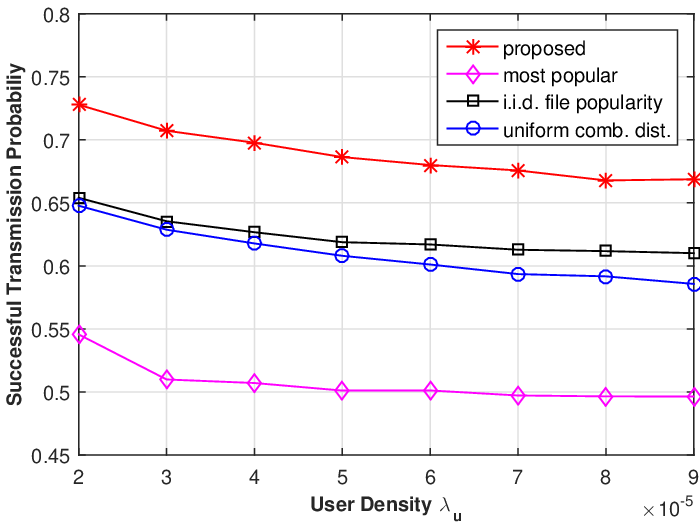
Fig. 5: Successful transmission probability versus cache size K1cK_{1}^{c} and K2cK_{2}^{c}, Zipf exponent γ\gamma and user density λu\lambda_{u}. K1c=K2c+10K_{1}^{c}=K_{2}^{c}+10, K1b=15K_{1}^{b}=15, λ1=5×10⁻⁷\lambda_{1}=5\times 10^{-7}, λ2=3×10⁻⁶\lambda_{2}=3\times 10^{-6}, P1P2=16\frac{P_{1}}{P_{2}}=16dB, α1=α2=4\alpha_{1}=\alpha_{2}=4, W=20×106W=20\times 10^{6}, τ=2×10⁴\tau=2\times 10^{4} and N=100N=100.

In this section, we compare the proposed near optimal design given by Algorithm 2 with three schemes. Baseline 1 (most popular) refers to the design in which each macro-BS selects the most K1c+K1bK_{1}^{c}+K_{1}^{b} popular files to store and fetch, and each pico-BS selects the most K2cK_{2}^{c} popular files to store [9, 10, 11]. Baseline 2 (i.i.d. file popularity) refers to the design in which each macro-BS selects K1c+K1bK_{1}^{c}+K_{1}^{b} files to store and fetch, and each pico-BS selects K2cK_{2}^{c} files to store, in an i.i.d. manner with file nn being selected with probability ana_{n} [19]. Note that under this scheme, each (macro or pico) BS may cache multiple copies of one file, leading to storage waste, and each macro-BS may fetch multiple copies of one file, leading to backhaul waste. Baseline 3 (uniform comb. dist.) refers to the design in which each macro-BS randomly selects a combination of K1c+K1bK_{1}^{c}+K_{1}^{b} different files to store and fetch, and each pico-BS randomly selects a combination of K2cK_{2}^{c} different files to store, according to the uniform distribution [13, 14]. Under the three baseline schemes, each user requesting file nn is associated with the BS which stores file nn and offers the maximum long-term average receive power at this user. In addition, the three baseline schemes also adopt the same multicasting scheme as in our design. In the simulation, we assume the popularity follows Zipf distribution, i.e., an=n−γ∑n∈𝒩n−γa_{n}=\frac{n^{-\gamma}}{\sum_{n\in\mathcal{N}}n^{-\gamma}}, where γ\gamma is the Zipf exponent.

Fig. 5 illustrates the successful transmission probability versus different parameters. From Fig. 5, we can observe that the proposed design outperforms all the three baseline schemes. In addition, the proposed design, Baseline 2 and Baseline 3 have much better performance than Baseline 1, as they provide file diversity to improve the network performance, when the storage and backhaul resources are limited and the cache-enabled HetNet with backhaul constraints may not be able to satisfy all file requests.

Specifically, Fig. 5 (a) illustrates the successful transmission probability versus the cache sizes K1cK_{1}^{c} and K2cK_{2}^{c}. We can see that the performance of all the schemes increases with K1cK_{1}^{c} and K2cK_{2}^{c}. This is because as K1cK_{1}^{c} and K2cK_{2}^{c} increase, each BS can store more files, and the probability that a randomly requested file is cached at a nearby BS increases. Fig. 5 (b) illustrates the successful transmission probability versus the Zipf exponent γ\gamma. We can observe that the performance of the proposed design, Baseline 1 and Baseline 2 increases with the Zipf exponent γ\gamma faster than Baseline 3. This is because when γ\gamma increases, the tail of popularity distribution becomes small, and hence, the average network file load decreases. The performance increase of Baseline 3 with γ\gamma only comes from the decrease of the average network file load. While, under the proposed design, Baseline 1 and Baseline 2, the probability that a randomly requested file is cached at a nearby BS increases with γ\gamma. Thus, the performance increases of the proposed design, Baseline 1 and Baseline 2 with γ\gamma are due to the decrease of the average network file load and the increase of the chance of a requested file being cached at a nearby BS. Fig. 5 (c) illustrates the successful transmission probability versus the user density λu\lambda_{u}. We can see that the performance of all the schemes decreases with λu\lambda_{u}. This is because the probability of a cached file being requested by at least one user increases, as λu\lambda_{u} increases.

IX Conclusion

In this paper, we considered the analysis and optimization of caching and multicasting in a large-scale cache-enabled HetNet with backhaul constraints. We proposed a hybrid caching design and a corresponding multicasting design to provide high spatial file diversity and ensure efficient content dissemination. Utilizing tools from stochastic geometry, we analyzed the successful transmission probability in the general region and the asymptotic region. Then, we formulated a mixed discrete-continuous optimization problem to maximize the successful transmission probability by optimizing the design parameters. By exploring the structural properties, we obtained a near optimal solution with superior performance and manageable complexity, based on a two-step optimization framework. The analysis and optimization results offered valuable design insights for practical cache-enabled HetNets.

Appendix A: Proof of Lemma 1

When typical user u0u_{0} requests file n∈ℱ1c∪ℱ1bn\in\mathcal{F}_{1}^{c}\cup\mathcal{F}_{1}^{b}, let random variable Ym,n∈{0,1}Y_{m,n}\in\{0,1\} denote whether file m∈ℱ1c∪ℱ1b∖{n}m\in\mathcal{F}_{1}^{c}\cup\mathcal{F}_{1}^{b}\setminus\{n\} is requested by the users associated with serving macro-BS ℓ0\ell_{0}. Specifically, when u0u_{0} requests file n∈ℱ1cn\in\mathcal{F}_{1}^{c}, we have K1,n,0c=1+∑m∈ℱ1c∖{n}Ym,nK_{1,n,0}^{c}=1+\sum_{m\in\mathcal{F}_{1}^{c}\setminus\{n\}}Y_{m,n} and K¯1,n,0b=∑m∈ℱ1bYm,n\overline{K}_{1,n,0}^{b}=\sum_{m\in\mathcal{F}_{1}^{b}}Y_{m,n}. When u0u_{0} requests file n∈ℱ1bn\in\mathcal{F}_{1}^{b}, we have K¯1,n,0c=∑m∈ℱ1cYm,n\overline{K}_{1,n,0}^{c}=\sum_{m\in\mathcal{F}_{1}^{c}}Y_{m,n} and K1,n,0b=1+∑m∈ℱ1b∖{n}Ym,nK_{1,n,0}^{b}=1+\sum_{m\in\mathcal{F}_{1}^{b}\setminus\{n\}}Y_{m,n}. Thus, we have

Pr[K1,n,0c=kc]=∑𝒳∈g⁡(ℱ1,−nc,kc−1)∏m∈𝒳(1−Pr[Ym,n=0])∏m∈ℱ1,−nc∖𝒳Pr[Ym,n=0],kc=1⋯K1c,\displaystyle\Pr\left[K_{1,n,0}^{c}=k^{c}\right]=\sum_{\mathcal{X}\in g(\mathcal{F}_{1,-n}^{c},k^{c}-1)}\prod_{m\in\mathcal{X}}(1-\Pr[Y_{m,n}=0])\prod_{m\in\mathcal{F}_{1,-n}^{c}\setminus\mathcal{X}}\Pr[Y_{m,n}=0],\hskip 9.24994ptk^{c}=1\cdots K_{1}^{c},
Pr[K¯1,n,0b=kb]=∑𝒳∈g⁡(ℱ1b,kb)∏m∈𝒳(1−Pr[Ym,n=0])∏m∈ℱ1b∖𝒳Pr[Ym,n=0],kb=0⋯F1b,\displaystyle\Pr\left[\overline{K}_{1,n,0}^{b}=k^{b}\right]=\sum_{\mathcal{X}\in g(\mathcal{F}_{1}^{b},k^{b})}\prod_{m\in\mathcal{X}}(1-\Pr[Y_{m,n}=0])\prod_{m\in\mathcal{F}_{1}^{b}\setminus\mathcal{X}}\Pr[Y_{m,n}=0],\hskip 9.24994ptk^{b}=0\cdots F_{1}^{b},
Pr[K¯1,n,0c=kc]=∑𝒳∈g⁡(ℱ1c,kc)∏m∈𝒳(1−Pr[Ym,n=0])∏m∈ℱ1c∖𝒳Pr[Ym,n=0],kc=0⋯K1c,\displaystyle\Pr\Big[\overline{K}_{1,n,0}^{c}=k^{c}\Big]=\sum_{\mathcal{X}\in g(\mathcal{F}_{1}^{c},k^{c})}\prod_{m\in\mathcal{X}}(1-\Pr[Y_{m,n}=0])\prod_{m\in\mathcal{F}_{1}^{c}\setminus\mathcal{X}}\Pr[Y_{m,n}=0],\hskip 9.24994ptk^{c}=0\cdots K_{1}^{c},
Pr[K1,n,0b=kb]=∑𝒳∈g⁡(ℱ1,−nb,kb−1)∏m∈𝒳(1−Pr[Ym,n=0])∏m∈ℱ1,−nb∖𝒳Pr[Ym,n=0],kb=1⋯F1b.\displaystyle\Pr\left[K_{1,n,0}^{b}=k^{b}\right]=\sum_{\mathcal{X}\in g(\mathcal{F}_{1,-n}^{b},k^{b}-1)}\prod_{m\in\mathcal{X}}(1-\Pr[Y_{m,n}=0])\prod_{m\in\mathcal{F}_{1,-n}^{b}\setminus\mathcal{X}}\Pr[Y_{m,n}=0],\hskip 9.24994ptk^{b}=1\cdots F_{1}^{b}.

To prove (10), (11), (12) and (13), it remains to calculate Pr[Ym,n=0]\Pr[Y_{m,n}=0]. The p.m.f. of Ym,nY_{m,n} depends on the p.d.f. of the size of the Voronoi cell of macro-BS ℓ0\ell_{0}, i.e., the p.d.f. of the size of the Voronoi cell to which a randomly chosen user belongs [25]. Thus, we can calculate the p.m.f. of Ym,nY_{m,n} using Lemma 3 of [25] as follows

Pr[Ym,n=0]=(1+3.5−1am​λuλ1)−4.5,m∈ℱ1c∪ℱ1b∖{n}.\displaystyle\Pr[Y_{m,n}=0]=\left(1+3.5^{-1}\frac{a_{m}\lambda_{u}}{\lambda_{1}}\right)^{-4.5},\hskip 9.24994pt\ m\in\mathcal{F}_{1}^{c}\cup\mathcal{F}_{1}^{b}\setminus\{n\}. (37)

Therefore, we complete the proof.

Appendix B: Proof of Lemma 2

When typical user u0u_{0} requests file n∈ℱ2cn\in\mathcal{F}_{2}^{c}, let random variable Ym,n,i∈{0,1}Y_{m,n,i}\in\{0,1\} denote whether file m∈𝒩i∖{n}m\in\mathcal{N}_{i}\setminus\{n\} is requested by the users associated with serving pico-BS ℓ0\ell_{0} when pico-BS ℓ0\ell_{0} contains combination i∈ℐni\in\mathcal{I}_{n}. When u0u_{0} requests file n∈ℱ2cn\in\mathcal{F}_{2}^{c} and serving pico-BS ℓ0\ell_{0} contains combination i∈ℐni\in\mathcal{I}_{n}, we have K2,n,0c=1+∑m∈𝒩i,−nYm,n,iK_{2,n,0}^{c}=1+\sum_{m\in\mathcal{N}_{i,-n}}Y_{m,n,i}. Thus, we have

Pr⁡[K2,n,0c=kc|pico-BS ℓ0 contains combination i∈ℐn]\displaystyle\Pr\left[K_{2,n,0}^{c}=k^{c}|\text{pico-BS $\ell_{0}$ contains combination $i\in\mathcal{I}_{n}$}\right]
=\displaystyle= ∑𝒳∈g⁡(𝒩i,−n,kc−1)∏m∈𝒳(1−Pr[Ym,n,i=0])∏m∈𝒩i,−n∖𝒳Pr[Ym,n,i=0],kc=1,⋯,K2c.\displaystyle\sum_{\mathcal{X}\in g\left(\mathcal{N}_{i,-n},k^{c}-1\right)}\prod_{m\in\mathcal{X}}(1-\Pr[Y_{m,n,i}=0])\prod_{m\in\mathcal{N}_{i,-n}\setminus\mathcal{X}}\Pr[Y_{m,n,i}=0],\hskip 9.24994ptk^{c}=1,\cdots,K_{2}^{c}. (38)

The probability that pico-BS ℓ0\ell_{0} contains combination i∈ℐni\in\mathcal{I}_{n} is piTn\frac{p_{i}}{T_{n}}. Thus, by the law of total probability, we have

Pr[K2,n,0c=kc]=∑i∈ℐnpiTnPr[K2,n,0c=kc|pico-BS ℓ0 contains combination i∈ℐn],kc=1,⋯,K2c.\displaystyle\Pr\left[K_{2,n,0}^{c}=k^{c}\right]=\sum_{i\in\mathcal{I}_{n}}\frac{p_{i}}{T_{n}}\Pr\left[K_{2,n,0}^{c}=k^{c}|\text{pico-BS $\ell_{0}$ contains combination $i\in\mathcal{I}_{n}$}\right],\hskip 9.24994ptk^{c}=1,\cdots,K_{2}^{c}.

Thus, to prove (14), it remains to calculate Pr[Ym,n,i=0]\Pr[Y_{m,n,i}=0]. The p.m.f. of Ym,n,iY_{m,n,i} depends on the p.d.f. of the size of the Voronoi cell of pico-BS ℓ0\ell_{0} w.r.t. file m∈𝒩i,−nm\in\mathcal{N}_{i,-n} when pico-BS ℓ0\ell_{0} contains combination i∈ℐni\in\mathcal{I}_{n}, which is unknown. We approximate this p.d.f. based on the known result of the p.d.f. of the size of the Voronoi cell to which a randomly chosen user belongs [25]. Under this approximation, we can calculate the p.m.f. of Ym,n,iY_{m,n,i} using Lemma 3 of [25] as follows

Pr[Ym,n,i=0]=\displaystyle\Pr[Y_{m,n,i}=0]= (1+3.5−1​am​λuTm​λ2)−4.5,m∈𝒩i,−n,i∈ℐn.\displaystyle\left(1+3.5^{-1}\frac{a_{m}\lambda_{u}}{T_{m}\lambda_{2}}\right)^{-4.5},\hskip 9.24994pt\ m\in\mathcal{N}_{i,-n},\ i\in\mathcal{I}_{n}. (39)

Appendix C: Proof of Theorem 1

Based on (7), to prove Theorem 1, we calculate q1​(ℱ1c,ℱ2c)q_{1}\left(\mathcal{F}_{1}^{c},\mathcal{F}_{2}^{c}\right) and q2​(ℱ2c,𝐩)q_{2}\left(\mathcal{F}_{2}^{c},\mathbf{p}\right), respectively.

Calculation of q1​(ℱ1c,ℱ2c)q_{1}\left(\mathcal{F}_{1}^{c},\mathcal{F}_{2}^{c}\right)

When u0u_{0} is a macro-user, as in the traditional connection-based HetNets, there are two types of interferers, namely, i) all the other macro-BSs besides its serving macro-BS, and ii) all the pico-BSs. Thus, we rewrite the SINR expression in (6) as follows:

SINRn,0=\displaystyle{\rm SINR}_{n,0}= D1,ℓ0,0−α1​|h1,ℓ0,0|2∑ℓ∈Φ1\{ℓ0}D1,ℓ,0−α1​|h1,ℓ,0|2+∑ℓ∈Φ2D2,ℓ,0−α2​|h2,ℓ,0|2​P2P1+N0P1=D1,ℓ0,0−α1​|h1,ℓ0,0|2I1+I2​P2P1+N0P1,n∈ℱ1c∪ℱ1b,\displaystyle\frac{{D_{1,\ell_{0},0}^{-\alpha_{1}}}\left|h_{1,\ell_{0},0}\right|^{2}}{\sum_{\ell\in\Phi_{1}\backslash\{\ell_{0}\}}D_{1,\ell,0}^{-\alpha_{1}}\left|h_{1,\ell,0}\right|^{2}+\sum_{\ell\in\Phi_{2}}D_{2,\ell,0}^{-\alpha_{2}}\left|h_{2,\ell,0}\right|^{2}\frac{P_{2}}{P_{1}}+\frac{N_{0}}{P_{1}}}=\frac{{D_{1,\ell_{0},0}^{-\alpha_{1}}}\left|h_{1,\ell_{0},0}\right|^{2}}{I_{1}+I_{2}\frac{P_{2}}{P_{1}}+\frac{N_{0}}{P_{1}}},\ n\in\mathcal{F}_{1}^{c}\cup\mathcal{F}_{1}^{b}, (40)

where I1≜∑ℓ∈Φ1\{ℓ0}D1,ℓ,0−α1​|h1,ℓ,0|2I_{1}\triangleq\sum_{\ell\in\Phi_{1}\backslash\{\ell_{0}\}}D_{1,\ell,0}^{-\alpha_{1}}\left|h_{1,\ell,0}\right|^{2} and I2≜∑ℓ∈Φ2D2,ℓ,0−α2​|h2,ℓ,0|2I_{2}\triangleq\sum_{\ell\in\Phi_{2}}D_{2,\ell,0}^{-\alpha_{2}}\left|h_{2,\ell,0}\right|^{2}.

Next, we calculate the conditional successful transmission probability of file n∈ℱ1c∪ℱ1bn\in\mathcal{F}_{1}^{c}\cup\mathcal{F}_{1}^{b} requested by u0u_{0} conditioned on D1,ℓ0,0=dD_{1,\ell_{0},0}=d when the file load is kk, i.e.,

qk,n,D1,ℓ0,0​(d)\displaystyle q_{k,n,D_{1,\ell_{0},0}}\left(d\right) ≜Pr⁡[Wk​log2⁡(1+SINRn,0)≥τ|D1,ℓ0,0=d]\displaystyle\triangleq{\rm Pr}\left[\frac{W}{k}\log_{2}\left(1+{\rm SINR}_{n,0}\right)\geq\tau\Big|D_{1,\ell_{0},0}=d\right]
=(a)EI1,I2​[Pr⁡[|h1,ℓ0,0|2≥(2k​τW−1)​D1,ℓ0,0α1​(I1+I2​P2P1+N0P1)|D1,ℓ0,0=d]]\displaystyle\stackrel{{\scriptstyle(a)}}{{=}}{\rm E}_{I_{1},I_{2}}\left[{\rm Pr}\left[\left|h_{1,\ell_{0},0}\right|^{2}\geq\left(2^{\frac{k\tau}{W}}-1\right)D_{1,\ell_{0},0}^{\alpha_{1}}\left(I_{1}+I_{2}\frac{P_{2}}{P_{1}}+\frac{N_{0}}{P_{1}}\right)\Big|D_{1,\ell_{0},0}=d\right]\right]
=(b)EI1,I2​[exp⁡(−(2k​τW−1)​dα1​(I1+I2​P2P1+N0P1))]\displaystyle\stackrel{{\scriptstyle(b)}}{{=}}{\rm E}_{I_{1},I_{2}}\left[\exp\left(-\left(2^{\frac{k\tau}{W}}-1\right)d^{\alpha_{1}}\left(I_{1}+I_{2}\frac{P_{2}}{P_{1}}+\frac{N_{0}}{P_{1}}\right)\right)\right]
=(c)EI1​[exp⁡(−(2k​τW−1)​dα1​I1)]⏟≜ℒI1​(s,d)|s=(2k​τW−1)​dα1​EI2​[exp⁡(−(2k​τW−1)​dα1​I2​P2P1)]⏟≜ℒI2​(s,d)|s=(2k​τW−1)​dα1\displaystyle\stackrel{{\scriptstyle(c)}}{{=}}\ \underbrace{{\rm E}_{I_{1}}\left[\exp\left(-\left(2^{\frac{k\tau}{W}}-1\right)d^{\alpha_{1}}I_{1}\right)\right]}_{\triangleq\mathcal{L}_{I_{1}}(s,d)|_{s=\left(2^{\frac{k\tau}{W}}-1\right)d^{\alpha_{1}}}}\underbrace{{\rm E}_{I_{2}}\left[\exp\left(-\left(2^{\frac{k\tau}{W}}-1\right)d^{\alpha_{1}}I_{2}\frac{P_{2}}{P_{1}}\right)\right]}_{\triangleq\mathcal{L}_{I_{2}}(s,d)|_{s=\left(2^{\frac{k\tau}{W}}-1\right)d^{\alpha_{1}}}}
×exp⁡(−(2k​τW−1)​dα1​N0P1),\displaystyle\hskip 22.76219pt\times\exp\left(-\left(2^{\frac{k\tau}{W}}-1\right)d^{\alpha_{1}}\frac{N_{0}}{P_{1}}\right), (41)

where (a)(a) is obtained based on (40), (b) is obtained by noting that |h1,ℓ0,0|2∼dexp⁡(1)|h_{1,\ell_{0},0}|^{2}\stackrel{{\scriptstyle d}}{{\sim}}\exp(1), and (c) is due to the independence of the Rayleigh fading channels and the independence of the PPPs. To calculate qk,n,D1,ℓ0,0​(d)q_{k,n,D_{1,\ell_{0},0}}\left(d\right) according to (41), we first calculate ℒI1​(s,d)\mathcal{L}_{I_{1}}(s,d) and ℒI2​(s,d)\mathcal{L}_{I_{2}}(s,d), respectively. The expression of ℒI1​(s,d)\mathcal{L}_{I_{1}}(s,d) is calculated as follows:

ℒI1​(s,d)\displaystyle\mathcal{L}_{I_{1}}(s,d) =E[exp(−s∑ℓ∈Φ1\{ℓ0}D1,ℓ,0−α1|h1,ℓ,0|2)]=E[∏ℓ∈Φ1\{ℓ0}exp(−sD1,ℓ,0−α1|h1,ℓ,0|2)]\displaystyle={\rm E}\left[\exp\left(-s\sum_{\ell\in\Phi_{1}\backslash\{\ell_{0}\}}D_{1,\ell,0}^{-\alpha_{1}}\left|h_{1,\ell,0}\right|^{2}\right)\right]={\rm E}\left[\prod_{\ell\in\Phi_{1}\backslash\{\ell_{0}\}}\exp\left(-sD_{1,\ell,0}^{-\alpha_{1}}\left|h_{1,\ell,0}\right|^{2}\right)\right]
=(d)exp(−2πλ1∫d∞(1−11+s​r−α1)rdr)\displaystyle\stackrel{{\scriptstyle(d)}}{{=}}\exp\left(-2\pi\lambda_{1}\int_{d}^{\infty}\left(1-\frac{1}{1+sr^{-\alpha_{1}}}\right)r{\rm d}r\right)
=(e)exp(−2​πα1λ1s2α1B′(2α1,1−2α1,11+s​d−α1)),\displaystyle\stackrel{{\scriptstyle(e)}}{{=}}\exp\left(-\frac{2\pi}{\alpha_{1}}\lambda_{1}s^{\frac{2}{\alpha_{1}}}B^{{}^{\prime}}\left(\frac{2}{\alpha_{1}},1-\frac{2}{\alpha_{1}},\frac{1}{1+sd^{-\alpha_{1}}}\right)\right), (42)

where (d)(d) is obtained by utilizing the probability generating functional of PPP [27, Page 235], and (e)(e) is obtained by first replacing s−1α1​rs^{-\frac{1}{\alpha_{1}}}r with tt, and then replacing 11+t−α1\frac{1}{1+t^{-\alpha_{1}}} with ww. Similarly, the expression of ℒI2​(s,d)\mathcal{L}_{I_{2}}(s,d) is calculated as follows:

ℒI2​(s,d)=\displaystyle\mathcal{L}_{I_{2}}(s,d)= E[exp(−s∑ℓ∈Φ2D2,ℓ,0−α2|h2,ℓ,0|2P2P1)]=E[∏ℓ∈Φ2exp(−sD2,ℓ,0−α2|h2,ℓ,0|2P2P1)]\displaystyle{\rm E}\left[\exp\left(-s\sum_{\ell\in\Phi_{2}}D_{2,\ell,0}^{-\alpha_{2}}\left|h_{2,\ell,0}\right|^{2}\frac{P_{2}}{P_{1}}\right)\right]={\rm E}\left[\prod_{\ell\in\Phi_{2}}\exp\left(-sD_{2,\ell,0}^{-\alpha_{2}}\left|h_{2,\ell,0}\right|^{2}\frac{P_{2}}{P_{1}}\right)\right]
=\displaystyle= exp(−2πλ2∫0∞(1−11+P2P1​s​r−α2)rdr)\displaystyle\exp\left(-2\pi\lambda_{2}\int_{0}^{\infty}\left(1-\frac{1}{1+\frac{P_{2}}{P_{1}}sr^{-\alpha_{2}}}\right)r{\rm d}r\right)
=\displaystyle= exp⁡(−2​πα2​λ2​(P2P1​s)2α2​B​(2α2,1−2α2)).\displaystyle\exp\left(-\frac{2\pi}{\alpha_{2}}\lambda_{2}\left(\frac{P_{2}}{P_{1}}s\right)^{\frac{2}{\alpha_{2}}}B\left(\frac{2}{\alpha_{2}},1-\frac{2}{\alpha_{2}}\right)\right)\;. (43)

Substituting (42) and (43) into (41), we obtain qk,n,D1,ℓ0,0​(d)q_{k,n,D_{1,\ell_{0},0}}\left(d\right) as follows:

qk,n,D1,ℓ0,0​(d)=\displaystyle q_{k,n,D_{1,\ell_{0},0}}\left(d\right)= exp(−2​πα1λ1d2(2k​τW−1)2α1B′(2α1,1−2α1,2−k​τW))exp(−(2k​τW−1)dα1N0P1)\displaystyle\exp\left(-\frac{2\pi}{\alpha_{1}}\lambda_{1}d^{2}\left(2^{\frac{k\tau}{W}}-1\right)^{\frac{2}{\alpha_{1}}}B^{{}^{\prime}}\left(\frac{2}{\alpha_{1}},1-\frac{2}{\alpha_{1}},2^{-\frac{k\tau}{W}}\right)\right)\exp\left(-\left(2^{\frac{k\tau}{W}}-1\right)d^{\alpha_{1}}\frac{N_{0}}{P_{1}}\right)
×exp⁡(−2​πα2​λ2​d2​α1α2​(P2P1​(2k​τW−1))2α2​B​(2α2,1−2α2)).\displaystyle\times\exp\left(-\frac{2\pi}{\alpha_{2}}\lambda_{2}d^{\frac{2\alpha_{1}}{\alpha_{2}}}\left(\frac{P_{2}}{P_{1}}\left(2^{\frac{k\tau}{W}}-1\right)\right)^{\frac{2}{\alpha_{2}}}B\left(\frac{2}{\alpha_{2}},1-\frac{2}{\alpha_{2}}\right)\right). (44)

Now, we calculate q1​(ℱ1c,ℱ2c)q_{1}\left(\mathcal{F}_{1}^{c},\mathcal{F}_{2}^{c}\right) by first removing the condition of qk,n,D1,ℓ0,0​(d)q_{k,n,D_{1,\ell_{0},0}}\left(d\right) on D1,ℓ0,0=dD_{1,\ell_{0},0}=d. Note that we have the p.d.f. of D1,ℓ0,0D_{1,\ell_{0},0} as fD1,ℓ0,0​(d)=2​π​λ1​d​exp⁡(−π​λ1​d2)f_{D_{1,\ell_{0},0}}(d)=2\pi\lambda_{1}d\exp\left(-\pi\lambda_{1}d^{2}\right). Thus, we have:

∫0∞qk,n,D1,ℓ0,0​(d)​fD1,ℓ0,0​(d)​𝑑d\displaystyle\int_{0}^{\infty}q_{k,n,D_{1,\ell_{0},0}}\left(d\right)f_{D_{1,\ell_{0},0}}(d){\rm d}d
=\displaystyle= 2πλ1∫0∞dexp(−2​πα1λ1d2(2k​τW−1)2α1B′(2α1,1−2α1,2−k​τW))exp(−(2k​τW−1)dα1N0P1)\displaystyle 2\pi\lambda_{1}\int_{0}^{\infty}d\exp\left(-\frac{2\pi}{\alpha_{1}}\lambda_{1}d^{2}\left(2^{\frac{k\tau}{W}}-1\right)^{\frac{2}{\alpha_{1}}}B^{{}^{\prime}}\left(\frac{2}{\alpha_{1}},1-\frac{2}{\alpha_{1}},2^{-\frac{k\tau}{W}}\right)\right)\exp\left(-\left(2^{\frac{k\tau}{W}}-1\right)d^{\alpha_{1}}\frac{N_{0}}{P_{1}}\right)
×exp⁡(−2​πα2​λ2​d2​α1α2​(P2P1​(2k​τW−1))2α2​B​(2α2,1−2α2))​exp⁡(−π​λ1​d2)​d​d.\displaystyle\times\exp\left(-\frac{2\pi}{\alpha_{2}}\lambda_{2}d^{\frac{2\alpha_{1}}{\alpha_{2}}}\left(\frac{P_{2}}{P_{1}}\left(2^{\frac{k\tau}{W}}-1\right)\right)^{\frac{2}{\alpha_{2}}}B\left(\frac{2}{\alpha_{2}},1-\frac{2}{\alpha_{2}}\right)\right)\exp\left(-\pi\lambda_{1}d^{2}\right){\rm d}d. (45)

Therefore, by (8) and by letting k=kc+kbk=k^{c}+k^{b} in (45), we have

q1​(ℱ1c,ℱ2c)=\displaystyle q_{1}\left(\mathcal{F}_{1}^{c},\mathcal{F}_{2}^{c}\right)= ∑n∈ℱ1can∑kc=1K1c∑kb=0F1bPr[K1,n,0c=kc]Pr[K¯1,n,0b=kb]∫0∞qk,n,D1,ℓ0,0(d)fD1,ℓ0,0(d)dd\displaystyle\sum_{n\in\mathcal{F}_{1}^{c}}a_{n}\sum_{k^{c}=1}^{K_{1}^{c}}\sum_{k^{b}=0}^{F_{1}^{b}}\Pr[K_{1,n,0}^{c}=k^{c}]\Pr[\overline{K}_{1,n,0}^{b}=k^{b}]\int_{0}^{\infty}q_{k,n,D_{1,\ell_{0},0}}\left(d\right)f_{D_{1,\ell_{0},0}}(d){\rm d}d
+∑n∈ℱ1ban∑kc=0K1c∑kb=1F1bPr[K¯1,n,0c=kc]Pr[K1,n,0b=kb]min⁡{K1b,kb}kb∫0∞qk,n,D1,ℓ0,0(d)fD1,ℓ0,0(d)dd.\displaystyle+\sum_{n\in\mathcal{F}_{1}^{b}}a_{n}\sum_{k^{c}=0}^{K_{1}^{c}}\sum_{k^{b}=1}^{F_{1}^{b}}\Pr[\overline{K}_{1,n,0}^{c}=k^{c}]\Pr[K_{1,n,0}^{b}=k^{b}]\frac{\min\{K_{1}^{b},k^{b}\}}{k^{b}}\int_{0}^{\infty}q_{k,n,D_{1,\ell_{0},0}}\left(d\right)f_{D_{1,\ell_{0},0}}(d){\rm d}d. (46)

Calculation of q2​(ℱ2c,𝐩)q_{2}\left(\mathcal{F}_{2}^{c},\mathbf{p}\right)

When u0u_{0} is a pico-user, different from the traditional connection-based HetNets, there are three types of interferers, namely, i) all the other pico-BSs storing the combinations containing the desired file of u0u_{0} besides its serving pico-BS, ii) all the pico-BSs without the desired file of u0u_{0}, and iii) all the macro-BSs. Thus, we rewrite the SINR expression in (6) as follows:

SINRn,0=\displaystyle{\rm SINR}_{n,0}= D2,ℓ0,0−α2​|h2,ℓ0,0|2∑ℓ∈Φ2,n\{ℓ0}D2,ℓ,0−α2​|h2,ℓ,0|2+∑ℓ∈Φ2,−nD2,ℓ,0−α2​|h2,ℓ,0|2+∑ℓ∈Φ1D1,ℓ,0−α1​|h1,ℓ,0|2​P1P2+N0P2\displaystyle\frac{{D_{2,\ell_{0},0}^{-\alpha_{2}}}\left|h_{2,\ell_{0},0}\right|^{2}}{\sum_{\ell\in\Phi_{2,n}\backslash\{\ell_{0}\}}D_{2,\ell,0}^{-\alpha_{2}}\left|h_{2,\ell,0}\right|^{2}+\sum_{\ell\in\Phi_{2,-n}}D_{2,\ell,0}^{-\alpha_{2}}\left|h_{2,\ell,0}\right|^{2}+\sum_{\ell\in\Phi_{1}}D_{1,\ell,0}^{-\alpha_{1}}\left|h_{1,\ell,0}\right|^{2}\frac{P_{1}}{P_{2}}+\frac{N_{0}}{P_{2}}}
=\displaystyle= D2,ℓ0,0−α2​|h2,ℓ0,0|2I2,n+I2,−n+I1​P1P2+N0P2,n∈𝒩,\displaystyle\frac{{D_{2,\ell_{0},0}^{-\alpha_{2}}}\left|h_{2,\ell_{0},0}\right|^{2}}{I_{2,n}+I_{2,-n}+I_{1}\frac{P_{1}}{P_{2}}+\frac{N_{0}}{P_{2}}},\ n\in\mathcal{N}, (47)

where Φ2,n\Phi_{2,n} is the point process generated by pico-BSs containing file combination i∈ℐni\in\mathcal{I}_{n}, Φ2,−n\Phi_{2,-n} is the point process generated by pico-BSs containing file combination i∉ℐni\not\in\mathcal{I}_{n}, I2,n≜∑ℓ∈Φ2,n\{ℓ0}D2,ℓ,0−α2​|h2,ℓ,0|2I_{2,n}\triangleq\sum_{\ell\in\Phi_{2,n}\backslash\{\ell_{0}\}}D_{2,\ell,0}^{-\alpha_{2}}\left|h_{2,\ell,0}\right|^{2}, I2,−n≜∑ℓ∈Φ2,−nD2,ℓ,0−α2​|h2,ℓ,0|2I_{2,-n}\triangleq\sum_{\ell\in\Phi_{2,-n}}D_{2,\ell,0}^{-\alpha_{2}}\left|h_{2,\ell,0}\right|^{2} and I1≜∑ℓ∈Φ1D1,ℓ,0−α1​|h1,ℓ,0|2I_{1}\triangleq\sum_{\ell\in\Phi_{1}}D_{1,\ell,0}^{-\alpha_{1}}\left|h_{1,\ell,0}\right|^{2}. Due to the random caching policy and independent thinning [27, Page 230], we obtain that Φ2,n\Phi_{2,n} is a homogeneous PPP with density λ2​Tn\lambda_{2}T_{n} and Φ2,−n\Phi_{2,-n} is a homogeneous PPP with density λ2​(1−Tn)\lambda_{2}\left(1-T_{n}\right).

Next, we calculate the conditional successful transmission probability of file n∈ℱ2cn\in\mathcal{F}_{2}^{c} requested by u0u_{0} conditioned on D2,ℓ0,0=dD_{2,\ell_{0},0}=d when the file load is kk, denoted as

qk,n,D2,ℓ0,0​(𝐩,d)≜Pr⁡[Wk​log2⁡(1+SINRn,0)≥τ|D2,ℓ0,0=d].q_{k,n,D_{2,\ell_{0},0}}\left({\bf p},d\right)\triangleq{\rm Pr}\left[\frac{W}{k}\log_{2}\left(1+{\rm SINR}_{n,0}\right)\geq\tau\Big|D_{2,\ell_{0},0}=d\right].

Similar to (41) and based on (47), we have:

qk,n,D2,ℓ0,0​(𝐩,d)\displaystyle q_{k,n,D_{2,\ell_{0},0}}\left({\bf p},d\right)
=EI2,n,I2,−n,I1​[Pr⁡[|h2,ℓ0,0|2≥(2k​τW−1)​D2,ℓ0,0α2​(I2,n+I2,−n+I1​P1P2+N0P2)|D2,ℓ0,0=d]]\displaystyle={\rm E}_{I_{2,n},I_{2,-n},I_{1}}\left[{\rm Pr}\left[\left|h_{2,\ell_{0},0}\right|^{2}\geq\left(2^{\frac{k\tau}{W}}-1\right)D_{2,\ell_{0},0}^{\alpha_{2}}\left(I_{2,n}+I_{2,-n}+I_{1}\frac{P_{1}}{P_{2}}+\frac{N_{0}}{P_{2}}\right)\Big|D_{2,\ell_{0},0}=d\right]\right]
=EI2,n​[exp⁡(−(2k​τW−1)​dα2​I2,n)]⏟≜ℒI2,n​(s,d)|s=(2k​τW−1)​dα2​EI2,−n​[exp⁡(−(2k​τW−1)​dα2​I2,−n)]⏟≜ℒI2,−n​(s,d)|s=(2k​τW−1)​dα2\displaystyle\hskip-85.35826pt=\underbrace{{\rm E}_{I_{2,n}}\left[\exp\left(-\left(2^{\frac{k\tau}{W}}-1\right)d^{\alpha_{2}}I_{2,n}\right)\right]}_{\triangleq\mathcal{L}_{I_{2,n}}(s,d)|_{s=\left(2^{\frac{k\tau}{W}}-1\right)d^{\alpha_{2}}}}\underbrace{{\rm E}_{I_{2,-n}}\left[\exp\left(-\left(2^{\frac{k\tau}{W}}-1\right)d^{\alpha_{2}}I_{2,-n}\right)\right]}_{\triangleq\mathcal{L}_{I_{2,-n}}(s,d)|_{s=\left(2^{\frac{k\tau}{W}}-1\right)d^{\alpha_{2}}}}
×EI1​[exp⁡(−(2k​τW−1)​dα2​I1​P1P2)]⏟≜ℒI1​(s,d)|s=(2k​τW−1)​dα2​exp⁡(−(2k​τW−1)​dα2​N0P2).\displaystyle\hskip-71.13188pt\times\underbrace{{\rm E}_{I_{1}}\left[\exp\left(-\left(2^{\frac{k\tau}{W}}-1\right)d^{\alpha_{2}}I_{1}\frac{P_{1}}{P_{2}}\right)\right]}_{\triangleq\mathcal{L}_{I_{1}}(s,d)|_{s=\left(2^{\frac{k\tau}{W}}-1\right)d^{\alpha_{2}}}}\exp\left(-\left(2^{\frac{k\tau}{W}}-1\right)d^{\alpha_{2}}\frac{N_{0}}{P_{2}}\right). (48)

To calculate qk,n,D2,ℓ0,0​(𝐩,d)q_{k,n,D_{2,\ell_{0},0}}\left({\bf p},d\right) according to (48), we first calculate ℒI2,n​(s,d)\mathcal{L}_{I_{2,n}}(s,d), ℒI2,−n​(s,d)\mathcal{L}_{I_{2,-n}}(s,d) and ℒI1​(s,d)\mathcal{L}_{I_{1}}(s,d) , respectively. Similar to (42) and (43), we have:

ℒI2,n(s,d)=exp(−2​πα2Tnλ2s2α2B′(2α2,1−2α2,11+s​d−α2)),\displaystyle\mathcal{L}_{I_{2,n}}(s,d)=\exp\left(-\frac{2\pi}{\alpha_{2}}T_{n}\lambda_{2}s^{\frac{2}{\alpha_{2}}}B^{{}^{\prime}}\left(\frac{2}{\alpha_{2}},1-\frac{2}{\alpha_{2}},\frac{1}{1+sd^{-\alpha_{2}}}\right)\right), (49)
ℒI2,−n​(s,d)=exp⁡(−2​πα2​(1−Tn)​λ2​s2α2​B​(2α2,1−2α2)),\displaystyle\mathcal{L}_{I_{2,-n}}(s,d)=\exp\left(-\frac{2\pi}{\alpha_{2}}(1-T_{n})\lambda_{2}s^{\frac{2}{\alpha_{2}}}B\left(\frac{2}{\alpha_{2}},1-\frac{2}{\alpha_{2}}\right)\right)\;, (50)
ℒI1​(s,d)=exp⁡(−2​πα1​λ1​(P1P2​s)2α1​B​(2α1,1−2α1)).\displaystyle\mathcal{L}_{I_{1}}(s,d)=\exp\left(-\frac{2\pi}{\alpha_{1}}\lambda_{1}\left(\frac{P_{1}}{P_{2}}s\right)^{\frac{2}{\alpha_{1}}}B\left(\frac{2}{\alpha_{1}},1-\frac{2}{\alpha_{1}}\right)\right)\;. (51)

Substituting (49), (50) and (51) into (48), we obtain qk,n,D2,ℓ0,0​(𝐩,d)q_{k,n,D_{2,\ell_{0},0}}\left({\bf p},d\right) as follows:

qk,n,D2,ℓ0,0​(𝐩,d)=\displaystyle q_{k,n,D_{2,\ell_{0},0}}\left({\bf p},d\right)= exp(−2​πα2Tnλ2d2(2k​τW−1)2α2B′(2α2,1−2α2,2−k​τW))exp(−(2k​τW−1)dα2N0P2)\displaystyle\exp\left(-\frac{2\pi}{\alpha_{2}}T_{n}\lambda_{2}d^{2}\left(2^{\frac{k\tau}{W}}-1\right)^{\frac{2}{\alpha_{2}}}B^{{}^{\prime}}\left(\frac{2}{\alpha_{2}},1-\frac{2}{\alpha_{2}},2^{-\frac{k\tau}{W}}\right)\right)\exp\left(-\left(2^{\frac{k\tau}{W}}-1\right)d^{\alpha_{2}}\frac{N_{0}}{P_{2}}\right)
×exp⁡(−2​πα2​(1−Tn)​λ2​d2​(2k​τW−1)2α2​B​(2α2,1−2α2))\displaystyle\times\exp\left(-\frac{2\pi}{\alpha_{2}}\left(1-T_{n}\right)\lambda_{2}d^{2}\left(2^{\frac{k\tau}{W}}-1\right)^{\frac{2}{\alpha_{2}}}B\left(\frac{2}{\alpha_{2}},1-\frac{2}{\alpha_{2}}\right)\right)
×exp⁡(−2​πα1​λ1​d2​α2α1​(P1P2​(2k​τW−1))2α1​B​(2α1,1−2α1)).\displaystyle\times\exp\left(-\frac{2\pi}{\alpha_{1}}\lambda_{1}d^{\frac{2\alpha_{2}}{\alpha_{1}}}\left(\frac{P_{1}}{P_{2}}\left(2^{\frac{k\tau}{W}}-1\right)\right)^{\frac{2}{\alpha_{1}}}B\left(\frac{2}{\alpha_{1}},1-\frac{2}{\alpha_{1}}\right)\right). (52)

Now, we calculate q2​(ℱ2c,𝐩)q_{2}\left(\mathcal{F}_{2}^{c},{\bf p}\right) by first removing the condition of qk,n,D2,ℓ0,0​(𝐩,d)q_{k,n,D_{2,\ell_{0},0}}\left({\bf p},d\right) on D2,ℓ0,0=dD_{2,\ell_{0},0}=d. Note that we have the p.d.f. of D2,ℓ0,0D_{2,\ell_{0},0} as fD2,ℓ0,0​(d)=2​π​Tn​λ2​d​exp⁡(−π​Tn​λ2​d2)f_{D_{2,\ell_{0},0}}(d)=2\pi T_{n}\lambda_{2}d\exp\left(-\pi T_{n}\lambda_{2}d^{2}\right), as pico-BSs storing file nn form a homogeneous PPP with density Tn​λ2T_{n}\lambda_{2}. Thus, we have:

∫0∞qk,n,D2,ℓ0,0​(𝐩,d)​fD2,ℓ0,0​(d)​𝑑d\displaystyle\int_{0}^{\infty}q_{k,n,D_{2,\ell_{0},0}}\left({\bf p},d\right)f_{D_{2,\ell_{0},0}}(d){\rm d}d
=\displaystyle= 2πTnλ2∫0∞dexp(−2​πα2Tnλ2d2(2k​τW−1)2α2B′(2α2,1−2α2,2−k​τW))exp(−(2k​τW−1)dα2N0P2)\displaystyle 2\pi T_{n}\lambda_{2}\int_{0}^{\infty}d\exp\left(-\frac{2\pi}{\alpha_{2}}T_{n}\lambda_{2}d^{2}\left(2^{\frac{k\tau}{W}}-1\right)^{\frac{2}{\alpha_{2}}}B^{{}^{\prime}}\left(\frac{2}{\alpha_{2}},1-\frac{2}{\alpha_{2}},2^{-\frac{k\tau}{W}}\right)\right)\exp\left(-\left(2^{\frac{k\tau}{W}}-1\right)d^{\alpha_{2}}\frac{N_{0}}{P_{2}}\right)
×exp⁡(−2​πα2​(1−Tn)​λ2​d2​(2k​τW−1)2α2​B​(2α2,1−2α2))​exp⁡(−π​Tn​λ2​d2)\displaystyle\times\exp\left(-\frac{2\pi}{\alpha_{2}}\left(1-T_{n}\right)\lambda_{2}d^{2}\left(2^{\frac{k\tau}{W}}-1\right)^{\frac{2}{\alpha_{2}}}B\left(\frac{2}{\alpha_{2}},1-\frac{2}{\alpha_{2}}\right)\right)\exp\left(-\pi T_{n}\lambda_{2}d^{2}\right)
×exp⁡(−2​πα1​λ1​d2​α2α1​(P1P2​(2k​τW−1))2α1​B​(2α1,1−2α1))​d​d.\displaystyle\times\exp\left(-\frac{2\pi}{\alpha_{1}}\lambda_{1}d^{\frac{2\alpha_{2}}{\alpha_{1}}}\left(\frac{P_{1}}{P_{2}}\left(2^{\frac{k\tau}{W}}-1\right)\right)^{\frac{2}{\alpha_{1}}}B\left(\frac{2}{\alpha_{1}},1-\frac{2}{\alpha_{1}}\right)\right){\rm d}d. (53)

Therefore, by (9) and by letting k=kck=k^{c} in (53), we have

q2(ℱ2c,𝐩)=∑n∈ℱ2can∑k=1K2cPr[K2,n,0c=kc]∫0∞qk,n,D2,ℓ0,0(𝐩,d)fD2,ℓ0,0(d)dd.\displaystyle q_{2}\left(\mathcal{F}_{2}^{c},{\bf p}\right)=\sum_{n\in\mathcal{F}_{2}^{c}}a_{n}\sum_{k=1}^{K_{2}^{c}}\Pr[K_{2,n,0}^{c}=k^{c}]\int_{0}^{\infty}q_{k,n,D_{2,\ell_{0},0}}\left({\bf p},d\right)f_{D_{2,\ell_{0},0}}(d){\rm d}d. (54)

Appendix D: Proof of Lemma 3 and Lemma 4

Proof of Lemma 3

When PN→∞\frac{P}{N}\to\infty, exp⁡(−(2k​τW−1)​dα​N0P1)→1\exp\left(-\left(2^{\frac{k\tau}{W}}-1\right)d^{\alpha}\frac{N_{0}}{P_{1}}\right)\to 1 and exp⁡(−(2k​τW−1)​dα​N0P2)→1\exp\left(-\left(2^{\frac{k\tau}{W}}-1\right)d^{\alpha}\frac{N_{0}}{P_{2}}\right)\to 1. When λu→∞\lambda_{u}\to\infty, discrete random variables K1,n,0c,K¯1,n,0c→K1cK_{1,n,0}^{c},\overline{K}_{1,n,0}^{c}\to K_{1}^{c}, K¯1,n,0b,K1,n,0b→F1b\overline{K}_{1,n,0}^{b},K_{1,n,0}^{b}\to F_{1}^{b} and K2,n,0c→K2cK_{2,n,0}^{c}\to K_{2}^{c} in distribution. Thus, when P1=β​PP_{1}=\beta P, P2=PP_{2}=P, PN0→∞\frac{P}{N_{0}}\to\infty, and λu→∞\lambda_{u}\to\infty, we can show f1,K1c+min⁡{K1b,F1b}→f1,K1c+min⁡{K1b,F1b},∞f_{1,K_{1}^{c}+\min\{K_{1}^{b},F_{1}^{b}\}}\to f_{1,K_{1}^{c}+\min\{K_{1}^{b},F_{1}^{b}\},\infty} and f2,K2c​(x)→f2,K2c,∞​(x)f_{2,K_{2}^{c}}(x)\to f_{2,K_{2}^{c},\infty}(x). Thus, we can prove Lemma 3.

Proof of Lemma 4

When P1=β​PP_{1}=\beta P, P2=PP_{2}=P, PN0→∞\frac{P}{N_{0}}\to\infty, λu→∞\lambda_{u}\to\infty, and α1=α2=α\alpha_{1}=\alpha_{2}=\alpha we have:

f1,K1c+min⁡{K1b,F1b},∞=\displaystyle f_{1,K_{1}^{c}+\min\{K_{1}^{b},F_{1}^{b}\},\infty}= 2​π​λ1​∫0∞d​exp⁡(−π​λ1​ωK1c+min⁡{K1b,F1b}​d2)​𝑑d=1ωK1c+min⁡{K1b,F1b},\displaystyle 2\pi\lambda_{1}\int_{0}^{\infty}d\exp\left(-\pi\lambda_{1}\omega_{K_{1}^{c}+\min\{K_{1}^{b},F_{1}^{b}\}}d^{2}\right){\rm d}d=\frac{1}{\omega_{K_{1}^{c}+\min\{K_{1}^{b},F_{1}^{b}\}}}, (55)
f2,K2c,∞​(x)=\displaystyle f_{2,K_{2}^{c},\infty}(x)= 2​π​λ2​∫0∞d​exp⁡(−π​λ2​d2​(θ2,K2c+x​θ1,K2c))​𝑑d=xθ2,K2c+θ1,K2c​x,\displaystyle 2\pi\lambda_{2}\int_{0}^{\infty}d\exp\left(-\pi\lambda_{2}d^{2}\left(\theta_{2,K_{2}^{c}}+x\theta_{1,K_{2}^{c}}\right)\right){\rm d}d=\frac{x}{\theta_{2,K_{2}^{c}}+\theta_{1,K_{2}^{c}}x}, (56)

where ωk\omega_{k}, θ1,k\theta_{1,k} and θ2,k\theta_{2,k} are given by (20), (21) and (22). Noting that ∫0∞d​exp⁡(−c​d2)​𝑑d=12​c\int_{0}^{\infty}d\exp\left(-cd^{2}\right){\rm d}d=\frac{1}{2c} (cc is a constant), we can solve integrals in (18) and (19). Thus, by Lemma 3, we can prove Lemma 4.

Appendix E: Proof of Lemma 5

To prove Lemma 5, we first have the following lemma.

Lemma 9 (Monotonicity of f2,k,∞​(x)f_{2,k,\infty}(x))

f2,k,∞​(x)f_{2,k,\infty}(x) is an increasing function of xx.

Proof:

By replacing exp⁡(−π​x​λ2​d2)\exp\left(-\pi x\lambda_{2}d^{2}\right) with yy in (19), we have:

f2,k,∞​(x)=\displaystyle f_{2,k,\infty}(x)= ∫01y−2α2(2k​τW−1)2α2(B(2α2,1−2α2)−B′(2α2,1−2α2,2−k​τW))y2α2​x​(2k​τW−1)2α2​B​(2α2,1−2α2)\displaystyle\int_{0}^{1}y^{-\frac{2}{\alpha_{2}}\left(2^{\frac{k\tau}{W}}-1\right)^{\frac{2}{\alpha_{2}}}\left(B\left(\frac{2}{\alpha_{2}},1-\frac{2}{\alpha_{2}}\right)-B^{{}^{\prime}}\left(\frac{2}{\alpha_{2}},1-\frac{2}{\alpha_{2}},2^{-\frac{k\tau}{W}}\right)\right)}y^{\frac{2}{\alpha_{2}x}\left(2^{\frac{k\tau}{W}}-1\right)^{\frac{2}{\alpha_{2}}}B\left(\frac{2}{\alpha_{2}},1-\frac{2}{\alpha_{2}}\right)}
×y(−ln⁡yπ​λ2)α2α1−1​2α1​(1x)α2α1​λ1λ2​(P1P2)2α1​(2k​τW−1)2α1​B​(2α1,1−2α1)​d​y.\displaystyle\times y^{\left(\frac{-\ln y}{\pi\lambda_{2}}\right)^{\frac{\alpha_{2}}{\alpha_{1}}-1}\frac{2}{\alpha_{1}}\left(\frac{1}{x}\right)^{\frac{\alpha_{2}}{\alpha_{1}}}\frac{\lambda_{1}}{\lambda_{2}}\left(\frac{P_{1}}{P_{2}}\right)^{\frac{2}{\alpha_{1}}}\left(2^{\frac{k\tau}{W}}-1\right)^{\frac{2}{\alpha_{1}}}B\left(\frac{2}{\alpha_{1}},1-\frac{2}{\alpha_{1}}\right)}{\rm d}y. (57)

When y∈(0,1)y\in(0,1) and a∈(0,∞)a\in\left(0,\infty\right), yay^{a} is a decreasing function of aa. Because B⁡(2α2,1−2α2)B\left(\frac{2}{\alpha_{2}},1-\frac{2}{\alpha_{2}}\right), B⁡(2α1,1−2α1)B\left(\frac{2}{\alpha_{1}},1-\frac{2}{\alpha_{1}}\right) and 2k​τW−1>02^{\frac{k\tau}{W}}-1>0, and 1x\frac{1}{x} and (1x)α2α1\left(\frac{1}{x}\right)^{\frac{\alpha_{2}}{\alpha_{1}}} are decreasing functions of xx. The integrand is an increasing function of xx for all y∈(0,1)y\in(0,1). Therefore, we can show that f2,k,∞​(x)f_{2,k,\infty}(x) is an increasing function of xx. ∎

Now, we prove Lemma 5. Let (ℱ1c∗,ℱ2c∗,𝐓∗)(\mathcal{F}_{1}^{c*},\mathcal{F}_{2}^{c*},\mathbf{T}^{*}) denote an optimal solution to Probelm 3. Consider n1,n2∈ℱ2c∗n_{1},n_{2}\in\mathcal{F}_{2}^{c*} satisfying an1>an2a_{n_{1}}>a_{n_{2}}. Suppose Tn1∗<Tn2∗T_{n_{1}}^{*}<T_{n_{2}}^{*}. Based on Lemma 9, we have f2,K2c,∞​(Tn1∗)<f2,K2c,∞​(Tn2∗)f_{2,K_{2}^{c},\infty}(T_{n_{1}}^{*})<f_{2,K_{2}^{c},\infty}(T_{n_{2}}^{*}). Now, we construct a feasible solution (ℱ1c′,ℱ2c′,𝐓′)(\mathcal{F}_{1}^{c^{\prime}},\mathcal{F}_{2}^{c^{\prime}},\mathbf{T}^{{}^{\prime}}) to Problem 3 by choosing ℱ1c′=ℱ1c∗\mathcal{F}_{1}^{c^{\prime}}=\mathcal{F}_{1}^{c*}, ℱ2c′=ℱ2c∗\mathcal{F}_{2}^{c^{\prime}}=\mathcal{F}_{2}^{c*}, Tn1′=Tn2∗,Tn2′=Tn1∗T_{n_{1}}^{\prime}=T_{n_{2}}^{*},T_{n_{2}}^{\prime}=T_{n_{1}}^{*}, and Tn′=Tn∗T_{n}^{{}^{\prime}}=T_{n}^{*} for all n∈ℱ2c∖{n1,n2}n\in\mathcal{F}_{2}^{c}\setminus\{n_{1},n_{2}\}. Thus, by Lemma 3 and the optimality of (ℱ1c∗,ℱ2c∗,𝐓∗)(\mathcal{F}_{1}^{c*},\mathcal{F}_{2}^{c*},\mathbf{T}^{*}), we have:

q∞(ℱ1c′,ℱ2c′,𝐓′)−q∞(ℱ1c∗,ℱ2c∗,𝐓∗)=(an1−an2)(f2,K2c,∞(Tn2∗)−f2,K2c,∞(Tn1∗))≤0.\displaystyle q_{\infty}\left(\mathcal{F}_{1}^{c^{\prime}},\mathcal{F}_{2}^{c^{\prime}},\mathbf{T}^{{}^{\prime}}\right)-q_{\infty}\left(\mathcal{F}_{1}^{c*},\mathcal{F}_{2}^{c*},\mathbf{T}^{*}\right)=\left(a_{n_{1}}-a_{n_{2}}\right)\left(f_{2,K_{2}^{c},\infty}(T_{n_{2}}^{*})-f_{2,K_{2}^{c},\infty}(T_{n_{1}}^{*})\right)\leq 0. (58)

Since an1>an2a_{n_{1}}>a_{n_{2}}, by (58), we have f2,K2c,∞​(Tn2∗)−f2,K2c,∞​(Tn1∗)≤0f_{2,K_{2}^{c},\infty}(T_{n_{2}}^{*})-f_{2,K_{2}^{c},\infty}(T_{n_{1}}^{*})\leq 0, which contradicts the assumption. Therefore, by contradiction, we can prove Lemma 5.

Appendix F: Proof of Lemma 6

For given ℱ2c\mathcal{F}_{2}^{c}, when α1=α2=α\alpha_{1}=\alpha_{2}=\alpha, PN0→∞\frac{P}{N_{0}}\to\infty, and λu→∞\lambda_{u}\to\infty, the Lagrangian of the optimization in (27) is given by

L⁡(𝐓,𝝀,𝜼,ν)=∑n∈ℱ2can​Tnθ2,K2c+θ1,K2c​Tn+∑n∈ℱ2cλn​Tn+∑n∈ℱ2cηn​(1−Tn)+ν⁡(K2c−∑n∈ℱ2cTn),L(\mathbf{T},\boldsymbol{\lambda},\boldsymbol{\eta},\nu)=\sum_{n\in\mathcal{F}_{2}^{c}}\frac{a_{n}T_{n}}{\theta_{2,K_{2}^{c}}+\theta_{1,K_{2}^{c}}T_{n}}+\sum_{n\in\mathcal{F}_{2}^{c}}\lambda_{n}T_{n}+\sum_{n\in\mathcal{F}_{2}^{c}}\eta_{n}(1-T_{n})+\nu\left(K_{2}^{c}-\sum_{n\in\mathcal{F}_{2}^{c}}T_{n}\right),

where λn\lambda_{n} and ηn≥0\eta_{n}\geq 0 are the Lagrange multipliers associated with (28), ν\nu is the Lagrange multiplier associated with (29), 𝝀≜(λn)n∈ℱ2c\boldsymbol{\lambda}\triangleq(\lambda_{n})_{n\in\mathcal{F}_{2}^{c}}, and 𝜼≜(ηn)n∈ℱ2c\boldsymbol{\eta}\triangleq(\eta_{n})_{n\in\mathcal{F}_{2}^{c}}. Thus, we have

∂L∂Tn​(𝐓,𝝀,𝜼,ν)=an​θ2,K2c(θ2,K2c+θ1,K2c​Tn)2+λn−ηn−ν.\frac{\partial L}{\partial T_{n}}(\mathbf{T},\boldsymbol{\lambda},\boldsymbol{\eta},\nu)=\frac{a_{n}\theta_{2,K_{2}^{c}}}{(\theta_{2,K_{2}^{c}}+\theta_{1,K_{2}^{c}}T_{n})^{2}}+\lambda_{n}-\eta_{n}-\nu.

Since strong duality holds, primal optimal 𝐓∗\mathbf{T}^{*} and dual optimal 𝝀∗\boldsymbol{\lambda}^{*}, 𝜼∗\boldsymbol{\eta}^{*}, ν∗\nu^{*} satisfy KKT conditions, i.e., (i) primal constraints: (28), (29), (ii) dual constraints λn≥0\lambda_{n}\geq 0 and ηn≥0\eta_{n}\geq 0 for all n∈ℱ2cn\in\mathcal{F}_{2}^{c}, (iii) complementary slackness λn​Tn=0\lambda_{n}T_{n}=0 and ηn​(1−Tn)=0\eta_{n}(1-T_{n})=0 for all n∈ℱ2cn\in\mathcal{F}_{2}^{c}, and (iv) an​θ2,K2c(θ2,K2c+θ1,K2c​Tn)2+λn−ηn−ν=0\frac{a_{n}\theta_{2,K_{2}^{c}}}{(\theta_{2,K_{2}^{c}}+\theta_{1,K_{2}^{c}}T_{n})^{2}}+\lambda_{n}-\eta_{n}-\nu=0 for all n∈ℱ2cn\in\mathcal{F}_{2}^{c}. By (ii), (iii), and (iv), when Tn=0T_{n}=0, we have λn≥0\lambda_{n}\geq 0, ηn=0\eta_{n}=0, and ν≥anθ2,K2c\nu\geq\frac{a_{n}}{\theta_{2,K_{2}^{c}}}; when 0<Tn<10<T_{n}<1, we have λn=0\lambda_{n}=0, ηn=0\eta_{n}=0, Tn=1θ1,K2c​an​θ2,K2cν−θ2,K2cθ1,K2cT_{n}=\frac{1}{\theta_{1,K_{2}^{c}}}\sqrt{\frac{a_{n}\theta_{2,K_{2}^{c}}}{\nu}}-\frac{\theta_{2,K_{2}^{c}}}{\theta_{1,K_{2}^{c}}}, and an​θ2,K2c(θ2,K2c+θ1,K2c)2<ν<anθ2,K2c\frac{a_{n}\theta_{2,K_{2}^{c}}}{(\theta_{2,K_{2}^{c}}+\theta_{1,K_{2}^{c}})^{2}}<\nu<\frac{a_{n}}{\theta_{2,K_{2}^{c}}}; when Tn=1T_{n}=1, we have λn=0\lambda_{n}=0, ηn≥0\eta_{n}\geq 0, and ν≤an​θ2,K2c(θ2,K2c+θ1,K2c)2\nu\leq\frac{a_{n}\theta_{2,K_{2}^{c}}}{(\theta_{2,K_{2}^{c}}+\theta_{1,K_{2}^{c}})^{2}}. Therefore, we have Tn∗=min⁡{[1θ1,K2c​an​θ2,K2cν∗−θ2,K2cθ1,K2c]+,1}T_{n}^{*}=\min\left\{\left[\frac{1}{\theta_{1,K_{2}^{c}}}\sqrt{\frac{a_{n}\theta_{2,K_{2}^{c}}}{\nu^{*}}}-\frac{\theta_{2,K_{2}^{c}}}{\theta_{1,K_{2}^{c}}}\right]^{+},1\right\}. Combining (29), we can prove Lemma 6.

Appendix G: Proof of Theorem 2

Proof of Property (i)(i) of Theorem 2

By constraints (1) and (5), we have K2c≤F2c∗K_{2}^{c}\leq F_{2}^{c*}, F2c∗=N−K1c−F1b∗F_{2}^{c*}=N-K_{1}^{c}-F_{1}^{b*} and 0≤F1b∗0\leq F_{1}^{b*}. To prove property (i) of Theorem 2, it remains to prove F1b∗≤K1bF_{1}^{b*}\leq K_{1}^{b}. Suppose there exists an optimal solution (ℱ1c∗,ℱ2c∗,𝐓∗)(\mathcal{F}_{1}^{c*},\mathcal{F}_{2}^{c*},\mathbf{T}^{*}) to Probelm 3 satisfying F1b∗>K1bF_{1}^{b*}>K_{1}^{b}, Then we have:

q∞∗=f1,K1c+K1b,∞(∑n∈ℱ1c∗an+K1b∑n∈ℱ1b∗anF1b∗)+∑n∈ℱ2c∗anf2,K2c,∞(Tn∗).\displaystyle q_{\infty}^{*}=f_{1,K_{1}^{c}+K_{1}^{b},\infty}\left(\sum_{n\in\mathcal{F}_{1}^{c*}}a_{n}+K_{1}^{b}\sum_{n\in\mathcal{F}_{1}^{b*}}\frac{a_{n}}{F_{1}^{b*}}\right)+\sum_{n\in\mathcal{F}_{2}^{c*}}a_{n}f_{2,K_{2}^{c},\infty}(T_{n}^{*}). (59)

Now, we construct a feasible solution (ℱ1c′,ℱ2c′,𝐓′)(\mathcal{F}_{1}^{c^{\prime}},\mathcal{F}_{2}^{c^{\prime}},\mathbf{T}^{{}^{\prime}}) to Problem 3, where ℱ1b′\mathcal{F}_{1}^{b^{\prime}} consists of the most K1bK_{1}^{b} popular files of ℱ1b∗\mathcal{F}_{1}^{b*}, ℱ1c′=ℱ1c∗\mathcal{F}_{1}^{c^{\prime}}=\mathcal{F}_{1}^{c*}, ℱ2c′=ℱ2c∗∪(ℱ1b∗∖ℱ1b′)\mathcal{F}_{2}^{c^{\prime}}=\mathcal{F}_{2}^{c*}\cup(\mathcal{F}_{1}^{b*}\setminus\mathcal{F}_{1}^{b^{\prime}}), Tn′=Tn∗T_{n}^{\prime}=T_{n}^{*} for all n∈ℱ2c∗n\in\mathcal{F}_{2}^{c*} and Tn′=0T_{n}^{\prime}=0 for all n∈ℱ1b∗∖ℱ1b′n\in\mathcal{F}_{1}^{b*}\setminus\mathcal{F}_{1}^{b^{\prime}}. By Lemma 3, we have:

q∞(ℱ1c′,ℱ2c′,𝐓′)−q∞∗=f1,K1c+K1b,∞(1K1b∑n∈ℱ1b′an−1F1b∑n∈ℱ1b∗an)K1b>0.\displaystyle q_{\infty}(\mathcal{F}_{1}^{c^{\prime}},\mathcal{F}_{2}^{c^{\prime}},\mathbf{T}^{{}^{\prime}})-q_{\infty}^{*}=f_{1,K_{1}^{c}+K_{1}^{b},\infty}\left(\frac{1}{K_{1}^{b}}\sum_{n\in\mathcal{F}_{1}^{b^{\prime}}}a_{n}-\frac{1}{F_{1}^{b}}\sum_{n\in\mathcal{F}_{1}^{b*}}a_{n}\right)K_{1}^{b}>0. (60)

Thus, (ℱ1c∗,ℱ2c∗,𝐓∗)(\mathcal{F}_{1}^{c*},\mathcal{F}_{2}^{c*},\mathbf{T}^{*}) is not an optimal solution, which contradicts the assumption. Therefore, by contradiction, we can prove F1b∗≤K1bF_{1}^{b*}\leq K_{1}^{b} for any optimal solution (ℱ1c∗,ℱ2c∗,𝐓∗)(\mathcal{F}_{1}^{c*},\mathcal{F}_{2}^{c*},\mathbf{T}^{*}) to Probelm 3. Since F2c∗≥K2cF_{2}^{c*}\geq K_{2}^{c}, F2c∗=N−K1c−F1b∗F_{2}^{c*}=N-K_{1}^{c}-F_{1}^{b*} and 0≤F1b∗≤K1b0\leq F_{1}^{b*}\leq K_{1}^{b}, we have max{K2c,N−K1c−K1b}≤F2c∗≤N−K1c\max\{K_{2}^{c},N-K_{1}^{c}-K_{1}^{b}\}\leq F_{2}^{c*}\leq N-K_{1}^{c}. Therefore, We can prove property (i) of Theorem 2.

Proof of Property (i​i)(ii) of Theorem 2

First, we prove that there exists an optimal solution (ℱ1c∗,ℱ2c∗,𝐓)(\mathcal{F}_{1}^{c*},\mathcal{F}_{2}^{c*},\mathbf{T}) to Problem 3, such that files in ℱ1c∗∪ℱ1b∗\mathcal{F}_{1}^{c*}\cup\mathcal{F}_{1}^{b*} are consecutive. By Lemma 3 and F1b∗≤K1bF_{1}^{b*}\leq K_{1}^{b} shown in the proof of Property(i)(i) , we have:

q∞∗=f1,K1c+F1b∗,∞∑n∈ℱ1c∗∪ℱ1b∗an+∑n∈ℱ2c∗anf2,K2c,∞(Tn∗).\displaystyle q_{\infty}^{*}=f_{1,K_{1}^{c}+F_{1}^{b*},\infty}\sum_{n\in\mathcal{F}_{1}^{c*}\cup\mathcal{F}_{1}^{b*}}a_{n}+\sum_{n\in\mathcal{F}_{2}^{c*}}a_{n}f_{2,K_{2}^{c},\infty}(T_{n}^{*}). (61)

Let n1​(n2)n_{1}(n_{2}) denote the most (least) popular file in ℱ1c∗∪ℱ1b∗\mathcal{F}_{1}^{c*}\cup\mathcal{F}_{1}^{b*}. Suppose for any optimal solution (ℱ1c∗,ℱ2c∗,𝐓∗)(\mathcal{F}_{1}^{c*},\mathcal{F}_{2}^{c*},\mathbf{T}^{*}) to Probelm 3, files in ℱ1c∗∪ℱ1b∗\mathcal{F}_{1}^{c*}\cup\mathcal{F}_{1}^{b*} are not consecutive, i.e., there exists n3∈ℱ2c∗n_{3}\in\mathcal{F}_{2}^{c*} satisfying n1<n3<n2n_{1}<n_{3}<n_{2}. Now, we can construct a feasible solution (ℱ1c′,ℱ2c′,𝐓′)(\mathcal{F}_{1}^{c^{\prime}},\mathcal{F}_{2}^{c^{\prime}},\mathbf{T}^{\prime}) to Probelm 3 where files in ℱ1c′∪ℱ1b′\mathcal{F}_{1}^{c^{\prime}}\cup\mathcal{F}_{1}^{b^{\prime}} are consecutive as follows.

∙\bullet If f1,K1c+F1b∗,∞<f2,K2c,∞(Tn3∗)f_{1,K_{1}^{c}+F_{1}^{b*},\infty}<f_{2,K_{2}^{c},\infty}(T_{n_{3}}^{*}), choose ℱ1c′∪ℱ1b′=ℱ1c∗∪ℱ1b∗∪{n3}∖{n1}\mathcal{F}_{1}^{c^{\prime}}\cup\mathcal{F}_{1}^{b^{\prime}}=\mathcal{F}_{1}^{c*}\cup\mathcal{F}_{1}^{b*}\cup\{n_{3}\}\setminus\{n_{1}\}, ℱ2c′=ℱ2c∗∪{n1}∖{n3}\mathcal{F}_{2}^{c^{\prime}}=\mathcal{F}_{2}^{c*}\cup\{n_{1}\}\setminus\{n_{3}\}, Tn1′=Tn3∗T_{n_{1}}^{\prime}=T_{n_{3}}^{*} and Tn′=Tn∗T_{n}^{\prime}=T_{n}^{*} for all n∈ℱ2c∗∖{n3}n\in\mathcal{F}_{2}^{c*}\setminus\{n_{3}\}. By Lemma 3, we have:

q∞(ℱ1c′,ℱ2c′,𝐓′)−q∞∗=(an1−an3)(f2,K2c,∞(Tn3∗)−f1,K1c+F1b∗,∞)>0,\displaystyle q_{\infty}\left(\mathcal{F}_{1}^{c^{\prime}},\mathcal{F}_{2}^{c^{\prime}},\mathbf{T}^{{}^{\prime}}\right)-q_{\infty}^{*}=\left(a_{n_{1}}-a_{n_{3}}\right)\left(f_{2,K_{2}^{c},\infty}(T_{n_{3}}^{*})-f_{1,K_{1}^{c}+F_{1}^{b*},\infty}\right)>0, (62)

where the inequality is due to n1<n3n_{1}<n_{3} and f1,K1c+F1b∗,∞<f2,K2c,∞(Tn3∗)f_{1,K_{1}^{c}+F_{1}^{b*},\infty}<f_{2,K_{2}^{c},\infty}(T_{n_{3}}^{*}).

∙\bullet If f1,K1c+F1b∗,∞>f2,K2c,∞(Tn3∗)f_{1,K_{1}^{c}+F_{1}^{b*},\infty}>f_{2,K_{2}^{c},\infty}(T_{n_{3}}^{*}), choose ℱ1c′∪ℱ1b′=ℱ1c∗∪ℱ1b∗∪{n3}∖{n2}\mathcal{F}_{1}^{c^{\prime}}\cup\mathcal{F}_{1}^{b^{\prime}}=\mathcal{F}_{1}^{c*}\cup\mathcal{F}_{1}^{b*}\cup\{n_{3}\}\setminus\{n_{2}\}, ℱ2c′=ℱ2c∗∪{n2}∖{n3}\mathcal{F}_{2}^{c^{\prime}}=\mathcal{F}_{2}^{c*}\cup\{n_{2}\}\setminus\{n_{3}\}, Tn2′=Tn3∗T_{n_{2}}^{\prime}=T_{n_{3}}^{*} and Tn′=Tn∗T_{n}^{\prime}=T_{n}^{*} for all n∈ℱ2c∗∖{n3}n\in\mathcal{F}_{2}^{c*}\setminus\{n_{3}\}. By Lemma 3, we have:

q∞(ℱ1c′,ℱ2c′,𝐓′)−q∞∗=(an2−an3)(f2,K2c,∞(Tn3∗)−f1,K1c+F1b∗,∞)>0,\displaystyle q_{\infty}\left(\mathcal{F}_{1}^{c^{\prime}},\mathcal{F}_{2}^{c^{\prime}},\mathbf{T}^{{}^{\prime}}\right)-q_{\infty}^{*}=\left(a_{n_{2}}-a_{n_{3}}\right)\left(f_{2,K_{2}^{c},\infty}(T_{n_{3}}^{*})-f_{1,K_{1}^{c}+F_{1}^{b*},\infty}\right)>0, (63)

where the inequality is due to n3<n2n_{3}<n_{2} and f2,K2c,∞(Tn3∗)<f1,K1c+F1b∗,∞f_{2,K_{2}^{c},\infty}(T_{n_{3}}^{*})<f_{1,K_{1}^{c}+F_{1}^{b*},\infty}.

∙\bullet If f1,K1c+F1b∗,∞=f2,K2c,∞(Tn3∗)f_{1,K_{1}^{c}+F_{1}^{b*},\infty}=f_{2,K_{2}^{c},\infty}(T_{n_{3}}^{*}), choose ℱ1c′∪ℱ1b′=ℱ1c∗∪ℱ1b∗∪{n3}∖{n1}\mathcal{F}_{1}^{c^{\prime}}\cup\mathcal{F}_{1}^{b^{\prime}}=\mathcal{F}_{1}^{c*}\cup\mathcal{F}_{1}^{b*}\cup\{n_{3}\}\setminus\{n_{1}\}, ℱ2c′=ℱ2c∗∪{n1}∖{n3}\mathcal{F}_{2}^{c^{\prime}}=\mathcal{F}_{2}^{c*}\cup\{n_{1}\}\setminus\{n_{3}\}, Tn1′=Tn3∗T_{n_{1}}^{\prime}=T_{n_{3}}^{*} and Tn′=Tn∗T_{n}^{\prime}=T_{n}^{*} for all n∈ℱ2c∗∖{n3}n\in\mathcal{F}_{2}^{c*}\setminus\{n_{3}\}. By Lemma 3, we have:

q∞(ℱ1c′,ℱ2c′,𝐓′)−q∞∗=(an1−an3)(f2,K2c,∞(Tn3∗)−f1,K1c+F1b∗,∞)=0,\displaystyle q_{\infty}\left(\mathcal{F}_{1}^{c^{\prime}},\mathcal{F}_{2}^{c^{\prime}},\mathbf{T}^{{}^{\prime}}\right)-q_{\infty}^{*}=\left(a_{n_{1}}-a_{n_{3}}\right)\left(f_{2,K_{2}^{c},\infty}(T_{n_{3}}^{*})-f_{1,K_{1}^{c}+F_{1}^{b*},\infty}\right)=0, (64)

By (62), (63) and (64), we know that if f1,K1c+F1b∗,∞<f2,K2c,∞(Tn3∗)f_{1,K_{1}^{c}+F_{1}^{b*},\infty}<f_{2,K_{2}^{c},\infty}(T_{n_{3}}^{*}) or f1,K1c+F1b∗,∞>f2,K2c,∞(Tn3∗)f_{1,K_{1}^{c}+F_{1}^{b*},\infty}>f_{2,K_{2}^{c},\infty}(T_{n_{3}}^{*}), (ℱ1c∗,ℱ2c∗,𝐓∗)(\mathcal{F}_{1}^{c*},\mathcal{F}_{2}^{c*},\mathbf{T}^{*}) is not an optimal solution, which contradicts the assumption; and if f1,K1c+F1b∗,∞=f2,K2c,∞(Tn3∗)f_{1,K_{1}^{c}+F_{1}^{b*},\infty}=f_{2,K_{2}^{c},\infty}(T_{n_{3}}^{*}), we can always construct an optimal solution (ℱ1c′,ℱ2c′,𝐓′)\left(\mathcal{F}_{1}^{c^{\prime}},\mathcal{F}_{2}^{c^{\prime}},\mathbf{T}^{{}^{\prime}}\right), satisfying that files in ℱ1c′∪ℱ1b′\mathcal{F}_{1}^{c^{\prime}}\cup\mathcal{F}_{1}^{b^{\prime}} are consecutive. Thus, we can prove that there exists an optimal solution (ℱ1c∗,ℱ2c∗,𝐓)(\mathcal{F}_{1}^{c*},\mathcal{F}_{2}^{c*},\mathbf{T}) to Problem 3, such that files in ℱ1c∗∪ℱ1b∗\mathcal{F}_{1}^{c*}\cup\mathcal{F}_{1}^{b*} are consecutive.

In addition, by (61), we know that whether file n∈ℱ1c∗∪ℱ1b∗n\in\mathcal{F}_{1}^{c*}\cup\mathcal{F}_{1}^{b*} belongs to ℱ1c∗\mathcal{F}_{1}^{c*} or ℱ1b∗\mathcal{F}_{1}^{b*} makes no difference in the optimal successful transmission probability. Therefore, we can prove the property (ii) of Theorem 2.

Appendix H: Proof of Lemma 7

Proof of Property (i)(i) of Lemma 7

We prove that if f1,K1c+K1b,∞>f2,K2c,∞​(1)f_{1,K_{1}^{c}+K_{1}^{b},\infty}>f_{2,K_{2}^{c},\infty}(1), the most popular file n=1n=1 belongs to ℱ1c∗∪ℱ1b∗\mathcal{F}_{1}^{c*}\cup\mathcal{F}_{1}^{b*} for any optimal solution (ℱ1c∗,ℱ2c∗,𝐓∗)\left(\mathcal{F}_{1}^{c*},\mathcal{F}_{2}^{c*},\mathbf{T}^{*}\right) to Problem 3. Suppose that there exists an optimal solution (ℱ1c∗,ℱ2c∗,𝐓∗)\left(\mathcal{F}_{1}^{c*},\mathcal{F}_{2}^{c*},\mathbf{T}^{*}\right) to Problem 3, such that the most popular file n=1n=1 belongs to ℱ2c∗\mathcal{F}_{2}^{c*}. Let n2n_{2} denote a file in ℱ1c∗∪ℱ1b∗\mathcal{F}_{1}^{c*}\cup\mathcal{F}_{1}^{b*}. Now, we can construct a feasible solution (ℱ1c′,ℱ2c′,𝐓′)(\mathcal{F}_{1}^{c^{\prime}},\mathcal{F}_{2}^{c^{\prime}},\mathbf{T}^{\prime}) to Probelm 3, where ℱ1c′∪ℱ1b′=ℱ1c∗∪ℱ1b∗∪{1}∖{n2}\mathcal{F}_{1}^{c^{\prime}}\cup\mathcal{F}_{1}^{b^{\prime}}=\mathcal{F}_{1}^{c*}\cup\mathcal{F}_{1}^{b*}\cup\{1\}\setminus\{n_{2}\}, ℱ2c′=ℱ2c∗∪{n2}∖{1}\mathcal{F}_{2}^{c^{\prime}}=\mathcal{F}_{2}^{c*}\cup\{n_{2}\}\setminus\{1\}, Tn2′=T1∗T_{n_{2}}^{\prime}=T_{1}^{*} and Tn′=Tn∗T_{n}^{\prime}=T_{n}^{*} for all n∈ℱ2c∗∖{1}n\in\mathcal{F}_{2}^{c*}\setminus\{1\}. By Lemma 3, we have:

q∞(ℱ1c′,ℱ2c′,𝐓′)−q∞∗=(a1−an2)(f1,K1c+min{K1b,F1b∗},∞−f2,K2c,∞(T1∗)).\displaystyle q_{\infty}\left(\mathcal{F}_{1}^{c^{\prime}},\mathcal{F}_{2}^{c^{\prime}},\mathbf{T}^{{}^{\prime}}\right)-q_{\infty}^{*}=\left(a_{1}-a_{n_{2}}\right)\left(f_{1,K_{1}^{c}+\min\{K_{1}^{b},F_{1}^{b*}\},\infty}-f_{2,K_{2}^{c},\infty}(T_{1}^{*})\right). (65)

Since a1>an2a_{1}>a_{n_{2}} and f1,K1c+min{K1b,F1b∗},∞≥f1,K1c+K1b,∞>f2,K2c,∞(1)≥f2,K2c,∞(T1∗)f_{1,K_{1}^{c}+\min\{K_{1}^{b},F_{1}^{b*}\},\infty}\geq f_{1,K_{1}^{c}+K_{1}^{b},\infty}>f_{2,K_{2}^{c},\infty}(1)\geq f_{2,K_{2}^{c},\infty}(T_{1}^{*}), we have q∞(ℱ1c′,ℱ2c′,𝐓′)−q∞∗>0q_{\infty}\left(\mathcal{F}_{1}^{c^{\prime}},\mathcal{F}_{2}^{c^{\prime}},\mathbf{T}^{{}^{\prime}}\right)-q_{\infty}^{*}>0. Thus, (ℱ1c∗,ℱ2c∗,𝐓∗)(\mathcal{F}_{1}^{c*},\mathcal{F}_{2}^{c*},\mathbf{T}^{*}) is not an optimal solution to Problem 3, which contradicts the assumption. By contradiction, we prove that if f1,K1c+K1b,∞>f2,K2c,∞​(1)f_{1,K_{1}^{c}+K_{1}^{b},\infty}>f_{2,K_{2}^{c},\infty}(1), the most popular file n=1n=1 belongs to ℱ1c∗∪ℱ1b∗\mathcal{F}_{1}^{c*}\cup\mathcal{F}_{1}^{b*} for any optimal solution (ℱ1c∗,ℱ2c∗,𝐓∗)\left(\mathcal{F}_{1}^{c*},\mathcal{F}_{2}^{c*},\mathbf{T}^{*}\right) to Problem 3, and hence n1cn_{1}^{c} in Theorem 2 (ii) satisfies n1c=1n_{1}^{c}=1.

Proof of Property (i​i)(ii) of Lemma 7

We prove that if f1,K1c,∞<f2,K2c,∞​(K2cN−K1c)f_{1,K_{1}^{c},\infty}<f_{2,K_{2}^{c},\infty}(\frac{K_{2}^{c}}{N-K_{1}^{c}}), the most popular file n=1n=1 belongs to ℱ2c∗\mathcal{F}_{2}^{c*} for any optimal solution (ℱ1c∗,ℱ2c∗,𝐓∗)\left(\mathcal{F}_{1}^{c*},\mathcal{F}_{2}^{c*},\mathbf{T}^{*}\right) to Problem 3. Suppose that there exists an optimal solution (ℱ1c∗,ℱ2c∗,𝐓∗)\left(\mathcal{F}_{1}^{c*},\mathcal{F}_{2}^{c*},\mathbf{T}^{*}\right) to Problem 3, such that file n=1n=1 belongs to ℱ1c∗∪ℱ1b∗\mathcal{F}_{1}^{c*}\cup\mathcal{F}_{1}^{b*}. Let n2n_{2} denote the most popular file in ℱ2c∗\mathcal{F}_{2}^{c*}. Based on Lemma 5, we have Tn2∗≥Tn∗T_{n_{2}}^{*}\geq T_{n}^{*} for any n∈ℱ2c∗∖{n2}n\in\mathcal{F}_{2}^{c*}\setminus\{n_{2}\}, and hence Tn2∗≥K2cN−K1cT_{n_{2}}^{*}\geq\frac{K_{2}^{c}}{N-K_{1}^{c}}. Now, we can construct a feasible solution (ℱ1c′,ℱ2c′,𝐓′)(\mathcal{F}_{1}^{c^{\prime}},\mathcal{F}_{2}^{c^{\prime}},\mathbf{T}^{\prime}) to Probelm 3, where ℱ1c′∪ℱ1b′=ℱ1c∗∪ℱ1b∗∪{n2}∖{1}\mathcal{F}_{1}^{c^{\prime}}\cup\mathcal{F}_{1}^{b^{\prime}}=\mathcal{F}_{1}^{c*}\cup\mathcal{F}_{1}^{b*}\cup\{n_{2}\}\setminus\{1\}, ℱ2c′=ℱ2c∗∪{1}∖{n2}\mathcal{F}_{2}^{c^{\prime}}=\mathcal{F}_{2}^{c*}\cup\{1\}\setminus\{n_{2}\}, T1′=Tn2∗T_{1}^{\prime}=T_{n_{2}}^{*} and Tn′=Tn∗T_{n}^{\prime}=T_{n}^{*} for all n∈ℱ2c∗∖{n2}n\in\mathcal{F}_{2}^{c*}\setminus\{n_{2}\}. By Lemma 3, we have:

q∞(ℱ1c′,ℱ2c′,𝐓′)−q∞∗=(a1−an2)(f2,K2c,∞(Tn2∗)−f1,K1c+min{K1b+ℱ1b∗},∞).\displaystyle q_{\infty}\left(\mathcal{F}_{1}^{c^{\prime}},\mathcal{F}_{2}^{c^{\prime}},\mathbf{T}^{{}^{\prime}}\right)-q_{\infty}^{*}=\left(a_{1}-a_{n_{2}}\right)\left(f_{2,K_{2}^{c},\infty}(T_{n_{2}}^{*})-f_{1,K_{1}^{c}+\min\{K_{1}^{b}+\mathcal{F}_{1}^{b*}\},\infty}\right). (66)

Since a1>an2a_{1}>a_{n_{2}} and f1,K1c+min{K1b+ℱ1b∗},∞≤f1,K1c,∞<f2,K2c,∞(K2cN−K1c)≤f2,K2c,∞(Tn2∗)f_{1,K_{1}^{c}+\min\{K_{1}^{b}+\mathcal{F}_{1}^{b*}\},\infty}\leq f_{1,K_{1}^{c},\infty}<f_{2,K_{2}^{c},\infty}(\frac{K_{2}^{c}}{N-K_{1}^{c}})\leq f_{2,K_{2}^{c},\infty}(T_{n_{2}}^{*}), we have q∞(ℱ1c′,ℱ2c′,𝐓′)−q∞∗>0q_{\infty}\left(\mathcal{F}_{1}^{c^{\prime}},\mathcal{F}_{2}^{c^{\prime}},\mathbf{T}^{{}^{\prime}}\right)-q_{\infty}^{*}>0. Thus, (ℱ1c∗,ℱ2c∗,𝐓∗)\left(\mathcal{F}_{1}^{c*},\mathcal{F}_{2}^{c*},\mathbf{T}^{*}\right) is not an optimal solution to Problem 3, which contradicts the assumption. Therefore, we prove that if f1,K1c,∞<f2,K2c,∞​(K2cN−K1c)f_{1,K_{1}^{c},\infty}<f_{2,K_{2}^{c},\infty}(\frac{K_{2}^{c}}{N-K_{1}^{c}}), the most popular file n=1n=1 belongs to ℱ2c∗\mathcal{F}_{2}^{c*} for any optimal solution (ℱ1c∗,ℱ2c∗,𝐓∗)\left(\mathcal{F}_{1}^{c*},\mathcal{F}_{2}^{c*},\mathbf{T}^{*}\right) to Problem 3, and hence n1cn_{1}^{c} in Theorem 2 (ii) satisfies n1c≥2n_{1}^{c}\geq 2.

References

  • [1] J. Hoadley and P. Maveddat, “Enabling small cell deployment with hetnet,” IEEE Wireless Communications, vol. 19, no. 2, pp. 4–5, April 2012.
  • [2] J. G. Andrews, “Seven ways that hetnets are a cellular paradigm shift,” IEEE Communications Magazine, vol. 51, no. 3, pp. 136–144, March 2013.
  • [3] X. Wang, M. Chen, T. Taleb, A. Ksentini, and V. Leung, “Cache in the air: exploiting content caching and delivery techniques for 5g systems,” Communications Magazine, IEEE, vol. 52, no. 2, pp. 131–139, February 2014.
  • [4] H. Sarkissian, “The business case for caching in 4g lte networks,” Wireless 20—20, vol. 20120, 2012.
  • [5] A. Liu and V. Lau, “Exploiting base station caching in MIMO cellular networks: Opportunistic cooperation for video streaming,” IEEE Trans. Signal Process., vol. 63, no. 1, pp. 57–69, Jan 2015.
  • [6] K. Shanmugam, N. Golrezaei, A. Dimakis, A. Molisch, and G. Caire, “Femtocaching: Wireless content delivery through distributed caching helpers,” Information Theory, IEEE Transactions on, vol. 59, no. 12, pp. 8402–8413, Dec 2013.
  • [7] J. Li, Y. Chen, Z. Lin, W. Chen, B. Vucetic, and L. Hanzo, “Distributed caching for data dissemination in the downlink of heterogeneous networks,” IEEE Transactions on Communications, vol. 63, no. 10, pp. 3553–3568, Oct 2015.
  • [8] V. Bioglio, F. Gabry, and I. Land, “Optimizing MDS codes for caching at the edge,” in 2015 IEEE Global Communications Conference (GLOBECOM), Dec 2015, pp. 1–6.
  • [9] E. Bastug˘\rm\breve{g}, M. Bennis, M. Kountouris, and M. Debbah, “Cache-enabled small cell networks: Modeling and tradeoffs,” EURASIP Journal on Wireless Communications and Networking, 2015.
  • [10] D. Liu and C. Yang, “Cache-enabled heterogeneous cellular networks: Comparison and tradeoffs,” in IEEE Int. Conf. on Commun. (ICC), Kuala Lumpur, Malaysia, June 2016. [Online]. Available: http://arxiv.org/abs/1602.08255
  • [11] C. Yang, Y. Yao, Z. Chen, and B. Xia, “Analysis on cache-enabled wireless heterogeneous networks,” Wireless Communications, IEEE Transactions on, vol. 15, no. 1, pp. 131–145, Jan 2016.
  • [12] Z. Chen, J. Lee, T. Q. S. Quek, and M. Kountouris, “Cooperative caching and transmission design in cluster-centric small cell networks,” CoRR, vol. abs/1601.00321, 2016. [Online]. Available: http://arxiv.org/abs/1601.00321
  • [13] S. T. ul Hassan, M. Bennis, P. H. J. Nardelli, and M. Latva-aho, “Caching in wireless small cell networks: A storage-bandwidth tradeoff,” IEEE Communications Letters, vol. PP, no. 99, pp. 1–1, 2016.
  • [14] S. Tamoor-ul-Hassan, M. Bennis, P. H. J. Nardelli, and M. Latva-aho, “Modeling and analysis of content caching in wireless small cell networks,” CoRR, vol. abs/1507.00182, 2015. [Online]. Available: http://arxiv.org/abs/1507.00182
  • [15] D. Lecompte and F. Gabin, “Evolved multimedia broadcast/multicast service (eMBMS) in LTE-advanced: overview and Rel-11 enhancements,” IEEE Commun. Mag., vol. 50, no. 11, pp. 68–74, 2012.
  • [16] K. Poularakis, G. Iosifidis, V. Sourlas, and L. Tassiulas, “Multicast-aware caching for small cell networks,” in IEEE WCNC, April 2014, pp. 2300–2305.
  • [17] B. Zhou, Y. Cui, and M. Tao, “Stochastic content-centric multicast scheduling for cache-enabled heterogeneous cellular networks,” submitted to Wireless Communications, IEEE Transactions on, vol. abs/1509.06611, 2015. [Online]. Available: http://arxiv.org/abs/1509.06611
  • [18] B. Blaszczyszyn and A. Giovanidis, “Optimal geographic caching in cellular networks,” in IEEE Int. Conf. on Commun. (ICC), London, United Kingdom, June 2015, pp. 1–6.
  • [19] B. N. Bharath and K. G. Nagananda, “Caching with unknown popularity profiles in small cell networks,” CoRR, vol. abs/1504.03632, 2015. [Online]. Available: http://arxiv.org/abs/1504.03632
  • [20] E. Altman, K. Avrachenkov, and J. Goseling, “Coding for caches in the plane,” CoRR, vol. abs/1309.0604, 2013. [Online]. Available: http://arxiv.org/abs/1309.0604
  • [21] Y. Cui, D. Jiang, and Y. Wu, “Analysis and optimization of caching and multicasting in large-scale cache-enabled wireless networks,” CoRR, vol. abs/1512.06176, 2015. [Online]. Available: http://arxiv.org/abs/1512.06176
  • [22] J. Andrews, F. Baccelli, and R. Ganti, “A tractable approach to coverage and rate in cellular networks,” Communications, IEEE Transactions on, vol. 59, no. 11, pp. 3122–3134, November 2011.
  • [23] S. Singh, H. S. Dhillon, and J. G. Andrews, “Offloading in heterogeneous networks: modeling, analysis, and design insights,” IEEE Trans. Wireless Commun., vol. 12, no. 5, pp. 2484–2497, March 2013.
  • [24] S. Singh and J. Andrews, “Joint resource partitioning and offloading in heterogeneous cellular networks,” Wireless Communications, IEEE Transactions on, vol. 13, no. 2, pp. 888–901, Feb 2014.
  • [25] S. M. Yu and S.-L. Kim, “Downlink capacity and base station density in cellular networks,” in Modeling Optimization in Mobile, Ad Hoc Wireless Networks (WiOpt), 2013 11th International Symposium on, May 2013, pp. 119–124.
  • [26] D. P. Bertsekas, Nonlinear Programming, 2nd ed. Belmont, MA: Athena Scientific, 1999.
  • [27] M. Haenggi and R. K. Ganti, “Interference in large wireless networks,” Foundations and Trends in Networking, vol. 3, no. 2, pp. 127–248, 2009.