Handling missing data in large healthcare dataset:
a case study of unknown trauma outcomes

E.M. Mirkes Email: em322@le.ac.uk Address: Department of Mathematics, University of Leicester, Leicester, LE1 7RH, UK T.J. Coats Email: tc61@le.ac.uk Address: Emergency Medicine Academic Group, Department of Cardiovascular Sciences, University of Leicester, Leicester, LE1 7RH, UK J. Levesley Email: jl1@le.ac.uk Address: Department of Mathematics, University of Leicester, Leicester, LE1 7RH, UK A.N. Gorban Email: ag153@le.ac.uk Address: Department of Mathematics, University of Leicester, Leicester, LE1 7RH, UK Corresponding author: Corresponding author

Abstract

Handling of missed data is one of the main tasks in data preprocessing especially in large public service datasets. We have analysed data from the Trauma Audit and Research Network (TARN) database, the largest trauma database in Europe. For the analysis we used 165,559 trauma cases. Among them, there are 19,289 cases (13.19%) with unknown outcome. We have demonstrated that these outcomes are not missed ‘completely at random’ and, hence, it is impossible just to exclude these cases from analysis despite the large amount of available data. We have developed a system of non-stationary Markov models for the handling of missed outcomes and validated these models on the data of 15,437 patients which arrived into TARN hospitals later than 24 hours but within 30 days from injury. We used these Markov models for the analysis of mortality. In particular, we corrected the observed fraction of death. Two naïve approaches give 7.20% (available case study) or 6.36% (if we assume that all unknown outcomes are ‘alive’). The corrected value is 6.78%. Following the seminal paper of Trunkey (1983) the multimodality of mortality curves has become a much discussed idea. For the whole analysed TARN dataset the coefficient of mortality monotonically decreases in time but the stratified analysis of the mortality gives a different result: for lower severities the coefficient of mortality is a non-monotonic function of the time after injury and may have maxima at the second and third weeks. The approach developed here can be applied to various healthcare datasets which experience the problem of lost patients and missed outcomes.

Keywords:

Missed data , Big data , Data cleaning , Mortality , Markov models , Risk evaluation

1 Introduction

Enthusiasm for the use of big data in the improvement of health service is huge but there is a concern that without proper attention to some specific challenges the mountain of big data efforts will bring forth a mouse [1]. Now, there is no technical problem with “big” in healthcare. Electronic health records include hundreds of millions of outpatient visits and tens of millions of hospitalizations, and these numbers grow exponentially. The main problem is in quality of data.

“Big data” very often means “dirty data” and the fraction of data inaccuracies increases with data volume growth. Human inspection at the big data scale is impossible and there is a desperate need for intelligent tools for accuracy and believability control.

The second big challenge of big data in healthcare is missed information. There may be many reasons for data incompleteness. One of them is in health service “fragmentation”. This problem can be solved partially by the national and international unification of the electronic health records (see, for example, Health Level Seven International (HL7) standards [2] or discussion of the template for uniform reporting of trauma data [3]). However, some fragmentation is unavoidable due to the diverse structure of the health service. In particular, the modern tendency for personalization of medicine can lead to highly individualized sets of attributes for different patients or patient groups. There are several universal technologies for the handling of missing data [4, 5, 6, 7, 8, 9, 10]. Nevertheless, the problem of handling missed values in large healthcare datasets is certainly not completely solved. It continues to attract the efforts of many researchers (see, for example, [11]) because the popular universal tools can lead to bias or loss of statistical power [12, 13]. For each system, it is desirable to combine various existing approaches for the handling of missing data (or to invent new ones) to minimize the damage to the results of data analysis. For the best possible solution, we have to take into account the peculiarities of each database and to specify the further use of the cleaned data (it is desirable to understand in advance how we will use the preprocessed data).

In our work we analyze missed values in the TARN database [14]. We use the preprocessed data for:

1.

the evaluation of the risk of death,
2.

the identification of the patterns of mortality,
3.

approaching several old problems like the Trunkey hypothesis about the trimodal distribution of trauma mortality [15].

The ‘two stage lottery’ non-stationary Markov model developed in the sequel can be used for the analysis of missing outcomes in a much wider context than the TARN database and could be applied to the handling of data gaps in healthcare datasets which experience the problem of transferred and lost patients and missing outcomes.

In this paper we analyze the unknown outcomes. The next task will be the analysis of missed data in the most common “input” attributes.

2 Data set

There are more than 200 hospitals which send information to TARN (TARN hospitals). This network is gradually increasing. Participation in TARN is recommended by the Royal College of Surgeons of England and the Department of Health. More than 93% of hospitals across England and Wales submit their data to TARN. TARN also receives data from Dublin, Waterford (Eire), Copenhagen, and Bern.

We use TARN data collected from 01.01.2008 (start of treatment) to 05.05.2014 (date of discharge). The database contains 192,623 records and more than 200 attributes. Sometimes several records correspond to the same trauma case because the patients may be transferred between TARN hospitals. We join these records. The resulting database includes data of 182,252 different trauma cases with various injuries.

Refer to caption — Figure 1: The groups of the patients for analysis of mortality. FOD in the group ‘Available W30D’ can be calculated from the data directly. Mortality in the group ‘OUT30’ will be evaluated on the basis of the non-stationary Markov model. The group of 16,693 patients which arrived (were transferred from other institutions) to TARN hospitals later than 24 hours after injury was excluded from the mortality analysis. Its subgroup ‘IN30’ of 15,437 patients is used for validation of the Markov model for ‘OUT30’ group. The subgroups with age $<65$ and age $\geq 65$ should be separated because for age $\geq 65$ the following traumas are excluded from the database: Acetabulum fractures (AIS 8562xx), Pelvic/Acetabulum fractures (AIS 8563xx), Pelvic ring fractures (AIS 8561xx), Pubic rami and Femoral neck fractures (AIS 85316x).

16,693 records correspond to patients, who arrived (transferred from other institutions) to TARN hospitals later than 24 hours after injury. This sample is biased, for example the Fraction Of Dead outcomes (FOD) for this sample is 3.34% and FOD for all data is 6.05%. This difference is very significant for such a big sample. (If all the outcomes in a group of the trauma cases are known then we use the simple definition of FOD in the group: the ratio of the number of registered deaths in this group to the total number of patients there. Such a definition is not always applicable. The detailed and more sophisticated analysis of this notion follows in the next section.) We remove these 16,693 trauma cases from analysis but use them later for validation of the “mortality after transfer” model. Among them, there are 15,437 patients who arrived at a TARN hospital within 30 days after injury. We call this group ‘IN30’ for short (Fig. 1).

As a result we have 165,559 records for analysis (‘Main group’). This main group consists of two subgroups: 146,270 patients from this group approached TARN during the first day of injury and remained in TARN hospitals or discharged to a final destination during the first 30 days after injury. We call this group the ‘Available within 30 days after injury’ cases (or ‘Available W30D’ for short). The other 19,289 patients have been transferred within 30 days after injury to a hospital or institution (or unknown destination) who did not return data to the TARN system. We call them ‘Transferred OUT OF TARN within 30 days after injury’ or just ‘OUT30’ (Fig. 1).

The patients with the non-final discharge destinations ‘Other Acute hospital’ and ‘Other institution’ were transferred from a TARN hospital to a hospital (institution) outside TARN and did not return to the TARN hospitals within 30 days after injury.

The database includes several indicators for evaluation of the severity of the trauma case, in particular, Abbreviated Injury Scale (AIS), Injury Severity Score (ISS) and New Injury Severity Score (NISS). For a detailed description and comparison of the scores we refer readers to reviews [16, 17]. The comparative study of predictive ability of different scores has a long history [18, 19, 20, 21]. The scores are used for mortality predictions and are tested on different datasets [22, 23, 24, 25]. In the database, there exist no gaps in AIS (and hence ISS and NISS) values even for patients rapidly dying. Most severely injured patients have a CT ‘pan-scan’ within the first hour or two of injury which is likely to define all life-threatening injuries. In addition the report from the post-mortem examination is used in the compilation of an injuries list which is the basis of AIS, and hence ISS and NISS, scoring.

3 Definitions and distributions of outcomes

The widely used definition of the endpoint outcome in trauma research is survival or death within 30 days after injury [26, 25, 27].

A substantial number of TARN in-hospital deaths following trauma occur after 30 days: there are 957 such cases (or 8% of TARN in-hospital death) among 11,900 cases with ‘Mortuary’ discharge destination. This proportion is practically the same in the main group (165,559 cases): 894 deaths after 30 days in hospital (or 7.9%) among 11,347 cases with ‘Mortuary’ discharge destination.

Death later than 30 days after injury may be considered as caused by co-morbidity rather than the direct consequence of the injury [25]. These later deaths are not very interesting from the perspective of an acute trauma care system (as we cannot influence them), but they might be very interesting from the perspective of a geriatric rehabilitation centre or of an injury prevention program for elderly patients.

On the other hand, when “end of acute care” is used as an outcome definition then a significant portion of deaths remains unnoticed. For example, in the 3332 trauma cases treated in the Ulleval University Hospital (Oslo, Norway, 2000-2004) 18% of deaths occurred after discharge from the hospital [27].

The question of whether it is possible to neglect trauma caused mortality within 30 days after trauma for the patients with the discharge destination ‘Home’, ‘Rehabilitation’ and other ‘recovery’ outcomes is not trivial [27]. Moreover, here are two questions:

1.

How do we collect all the necessary data after discharge within 30 days after trauma – a technical question?
2.

How do we classify the death cases after discharge within 30 days after trauma; are they consequences of the trauma or should they be considered as comorbidity with some additional reasons?

The best possible answer to the first question requires the special combination of technical and business process to integrate data from different sources. The recent linkage from TARN to the Office for National Statistics (ONS) gives the possibility to access the information about the dates of death in many cases. It is expected that the further data integration process will recover many gaps in the outcome data.

The last question is far beyond the scope of data management and analysis and may be approached from different perspectives. Whether or not the late deaths are important in a model depends on the question being asked. From the data management perspective, we have to give the formal definition of the outcome in the terms of the available database fields. It is impossible to use the standard definition as survival or death within 30 days after injury because these data are absent. We define the outcome ‘Alive W30D’ for the TARN database being as close to the standard definition as it is possible.

In the TARN database discharge destinations ‘Home (own)’, ‘Home (relative or other carer)’, ‘Nursing Home’, and ‘Rehabilitation’ are considered as final. If we assume that these trauma cases have the outcome ‘Alive W30D’ then we loose some cases of death. From the acute care perspective these cases can be considered as irrelevant. Let us accept this definition. There still remain many cases with unknown outcome. For analysis of these cases we introduce the outcome category ‘Transferred’. In this category we include the cases which left the TARN registry to a hospital or other institution outside TARN, or to an unknown destination within 30 days. The relations between the discharge destinations and these three outcomes are presented in Table 1.

Table 1: Distribution of outcomes in the main group (W30D means within 30 days after injury).

Subgroup	Alive W30D	Dead W30D	Unknown	Total
Available W30D	135,733	10,537	0	146,270
OUT30	0^∗	0^∗	19,279	19,289
Total	135,733	10,537	19,289	165,559

^∗No known survival or deaths.

As we can see from Table 1, 19,289 trauma cases (or 11.35% of all cases) have unknown outcome. The first standard question is: can we delete these data and apply available case analysis? For this purpose we have to consider these outcome data as “Missing Completely at Random” (MCAR) [28, 4, 6, 7]. This is definitely not the case. The group with unknown outcomes is exactly the ‘OUT30’ group. The probability of belonging to this group depends, for example, on the severity of injury (which can be measured, by the maximal severity, by NISS, by GCS or by another severity score). The $\chi^{2}$ test of independence shows that transfer depends on the severity with $p$ -value $p<10^{-300}$ (this is the probability that such a strong dependence might appear by chance). The most practical (or ‘purposefull’ [29]) idea is to consider the missed outcome data as “Missed at Random” (MAR). The assumption of MAR does not imply that the data are missing randomly, but rather that the missing values are correlated with variables recorded in the dataset [29].

One can consider all these cases as alive because these patients have been alive at the point of discharge from TARN hospitals. If we consider all transferred as alive then the FOD is 6.35%. If we delete all the transferred patients (study only the Available W30D group) then the FOD is 7.2%. If we test this hypothesis on 15,437 patients of the group ‘IN30’ transferred to TARN hospitals from outside the network within 30 days after injury then we find that the nonzero mortality for them (3.10%).

The data table with known outcomes is necessary for further machine learning and the main goal is outcome prediction and risk evaluation.

We choose to remove the OUT30D group from data table but simultaneously to adjust the weights of the retained cases to compensate for the removal. The information about the OUT30D cases will be used in the construction of the weights. It is necessary to evaluate the mortality of the patients transferred from TARN before removing their records and reweighting of the rest. In the next section we develop, identify and validate Markov models for the analysis of the mortality of transferred patients.

Another method for handling missed outcomes is multiple imputation of the outcomes (about multiple imputations see, for example, [9]). Both methods use similar stochastic models of mortality and transfer. The large number of cases allows us to use the reweighting approach. A significant majority of the evaluated weights are between 0.9 and 1.1 (see Section 6).

4 Non-stationary Markov model for the analysis of missing outcomes

4.1 Structure of model

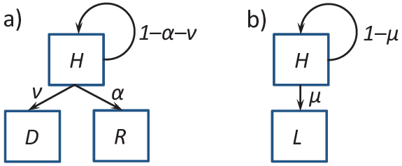
We propose a system of Markov models for evaluation of mortality in trauma datasets. In these models each day each patient can participate in two ‘lotteries’ (Fig. 2). The first lottery (recovery/death), Fig. 2 a, has three outcomes: ‘R’ (recovery), ‘D’ (death), and ‘H’ (remains in a TARN hospital). The second lottery (of transfer), Fig. 2 b, has two outcomes: ‘H’ (remains in a TARN hospital) and ‘L’ (transfer from the TARN hospital to a hospital or ‘other institution’ outside TARN). The probabilities of outcomes depend on the time from the injury $t$ and on the state of the patient after injury $s$ . It is important to stress that $s$ in our models characterizes the state of the patient on the first day after trauma and may include severity, type of injury (blunt/penetrating), localization of traumas, age, gender, airway status, systolic and diastolic blood pressure, etc, but cannot change in time.

The description of state $s$ may vary in the level of detail depending on the available information. We have fitted and tested two models based on the severity of trauma: the maximal severity model and the (binned) NISS model. In Section 5 we demostrate that it is necessary to refine the model and to include the age group in $s$ for low severities. For different purposes the mortality model can include more detail.

The lotteries (Fig. 2) do not commute. We consider two limit cases: ‘advanced transfer’ (Fig. 3) and ‘retarded transfer’ (Fig. 4). In models with advanced transfer the lottery of transfer Fig. 2 b) each day precedes the lottery of recovery/death (Fig. 2 a). In models with retarded transfer, conversely, the lottery of recovery/death precedes the lottery of transfer.

These two models are important because many other much more general Markov models are between them in the following exact sense. It is a very strong assumption that every day there are two steps only: the recovery/death lottery and the transfer lottery. It may be more realistic to assume that every day there are many ‘fractional steps’ of recovery/death and of transfer from TARN and the result of the day is the aggregate result of all of these fractional steps. Assume that the events of recover, death and transfer are sampled for every day after injury $t$ from a number $M$ consecutive random choices with probabilities $\alpha_{i},\nu_{i}$ for recovery/death and $\mu_{i}$ for transfer out of TARN ( $i=1,\ldots,M$ ), and this chain of choices is Markovian (the choices for a patient do not depend on the previous choices directly but only on the current state, H, R or L). It is non-stationary because the transition probabilities depend on time. They are different for different days after injury.

This sequence of choices is displayed as a sequence of fractional steps:

\begin{split}\mbox{recovery/death}_{1}&\to\mbox{transfer}_{1}\to\ldots\\ &\to\mbox{recovery/death}_{M}\to\mbox{transfer}_{M}.\end{split}

The probability of in-TARN death in the above model of sequential choice, on a given day after trauma is

\nu_{1}+\nu_{2}(1-\alpha_{1}-\nu_{1})(1-\mu_{1})+\ldots+\nu_{M}\prod_{i=1}^{M-1}(1-\alpha_{i}-\nu_{i})(1-\mu_{i}).

Similarly, the probability for recovery is

\alpha_{1}+\alpha_{2}(1-\alpha_{1}-\nu_{1})(1-\mu_{1})+\ldots+\alpha_{M}\prod_{i=1}^{M-1}(1-\alpha_{i}-\nu_{i})(1-\mu_{i}).

Finally, the probability of transfer to a hospital outside of TARN is

\begin{split}\mu_{1}(1-\alpha_{1}-\nu_{1})&+\mu_{2}(1-\mu_{1})(1-\alpha_{1}-\nu_{1})(1-\alpha_{2}-\nu_{2})\\ &+\ldots+\mu_{M}\prod_{i=1}^{M-1}(1-\mu_{i})\prod_{j=1}^{M}(1-\alpha_{j}-\nu_{j}){.}\end{split}

The probabilities $\alpha_{i},\nu_{i}$ for the fractional steps should be consistent with the daily probabilities $\alpha,\nu$ : if there is no transfer then the resulting probabilities of recovery or death should be the same:

\begin{split}&\alpha_{1}+\alpha_{2}(1-\alpha_{1}-\nu_{1})+\ldots+\alpha_{M}\prod_{i=1}^{M-1}(1-\alpha_{i}-\nu_{i})=\alpha,\\ &\nu_{1}+\nu_{2}(1-\alpha_{1}-\nu_{1})+\ldots+\nu_{M}\prod_{i=1}^{M-1}(1-\alpha_{i}-\nu_{i})=\nu.\\ &\mbox{{Also,} }\prod_{i=1}^{M}(1-\alpha_{i}-\nu_{i})=1-\alpha-\nu.\end{split}

(1)

Similarly, for $\mu_{i}$ we get the conditions

\begin{split}\mu_{1}+\mu_{2}(1-\mu_{1})+\ldots+\mu_{M}\prod_{i=1}^{M-1}(1-\mu_{i})&=\mu\\ \mbox{ {and} }\prod_{i=1}^{M}(1-\mu_{i})&=1-\mu{.}\end{split}

(2)

Proposition 1.

The probability of in-TARN death in the described model of sequential choice for every day after trauma is between the probabilities for the Markovian model with advanced transfer (Fig. 3) and the Markovian model with retarded transfer (Fig. 4):

\begin{split}\nu(1-\mu)\leq\nu_{1}&+\nu_{2}(1-\alpha_{1}-\nu_{1})(1-\mu_{1})+\ldots\\ &+\nu_{M}\prod_{i=1}^{M-1}(1-\alpha_{i}-\nu_{i})(1-\mu_{i})\leq\nu.\end{split}

(3)

Proof.

According to conditions (1), (2),

\begin{split}&\nu(1-\mu)\\ &=\left[\nu_{1}+\nu_{2}(1-\alpha_{1}-\nu_{1})+\ldots+\nu_{M}\prod_{i=1}^{M-1}(1-\alpha_{i}-\nu_{i})\right]\\ &\quad\times\prod_{i=1}^{M}(1-\mu_{i}).\end{split}

(4)

Notice that for every $j$ ( $1\leq j\leq M$ ),

\prod_{i=1}^{M}(1-\mu_{i})\leq\prod_{i=1}^{j}(1-\mu_{i})

because $0\leq 1-\mu_{i}\leq 1$ for all probabilities $\mu_{i}$ . Therefore,

\nu_{j}\prod_{i=1}^{j}(1-\alpha_{i}-\nu_{i})\prod_{k=1}^{M}(1-\mu_{k})\leq\nu_{j}\prod_{i=1}^{j}(1-\alpha_{i}-\nu_{i})(1-\mu_{i})

and the following inequality holds

\begin{split}&\left[\nu_{1}+\nu_{2}(1-\alpha_{1}-\nu_{1})+\ldots+\nu_{M}\prod_{i=1}^{M-1}(1-\alpha_{i}-\nu_{i})\right]\\ &\times\prod_{i=1}^{M}(1-\mu_{i})\\ &\leq\nu_{1}+\nu_{2}(1-\alpha_{1}-\nu_{1})+\ldots+\nu_{M}\prod_{i=1}^{M-1}(1-\alpha_{i}-\nu_{i}).\end{split}

(5)

The left inequality in (3) is proven. The right inequality in (3) follows from condition (1) because for every product

\nu_{j}\prod_{i=1}^{j}(1-\alpha_{i}-\nu_{i})(1-\mu_{i})\leq\nu_{j}\prod_{i=1}^{j}(1-\alpha_{i}-\nu_{i}){.}

∎

The proofs of the following propositions are very similar

Proposition 2.

The probability of in-TARN recovery in the described model of sequential choice for every day after trauma is between the probabilities for the Markovian model with advanced transfer (Fig. 3) and the Markovian model with retarded transfer (Fig. 4):

\begin{split}\alpha(1-\mu)\leq\alpha_{1}&+\alpha_{2}(1-\alpha_{1}-\nu_{1})(1-\mu_{1})+\ldots\\ &+\alpha_{M}\prod_{i=1}^{M-1}(1-\alpha_{i}-\nu_{i})(1-\mu_{i})\leq\alpha{.}\end{split}

(6)

$\square$

Proposition 3.

The probability of transfer outside TARN in the described model of sequential choice for every day after trauma is between the probabilities for the Markovian model with advanced transfer (Fig. 3) and the Markovian model with retarded transfer (Fig. 4):

\mu(1-\alpha-\nu)\leq\sum_{j=1}^{M}\mu_{j}(1-\alpha_{j}-\nu_{j})\prod_{i=1}^{j-1}(1-\alpha_{i}-\nu_{i})(1-\mu_{i})\leq\mu{.}

(7)

$\square$

4.2 Transition probabilities and their evaluation

In the above models (Figs. 3 and 4), death and recovery of the transferred patients have the same probabilities as for the patients of TARN hospitals. These probabilities are defined by the state of the patient $s$ and by the time after injury. Of course, in reality there is often a hope that the transfer will improve the situation and the probability of death will decrease for the same state of the patient. Nevertheless, in this paper we will neglect the changes of probabilities after transfer (just because we have no sufficient reason for such a change). Of course, these models could be extended to include the changes of mortality for transferred patients, if necessary.

Another question is the definition of $s$ . Which attributes should be included in the ‘state’ for the models (Figs. 3, 4)? To motivate this choice, we should take into account two considerations:

1.

The models will be used to analyse data with unknown outcomes. Trauma cases with missed outcomes make up 10-12% of the dataset. Therefore, an error of 10% in mortality for data with unknown outcomes will cause an error of $\sim$ 1% in mortality for the whole dataset and it is possible to use relatively coarse models (see below).
2.

The description of the state $s$ should include attributes whose values are known for a significant majority of cases. This is especially important because for cases with unknown outcomes many of the attributes are often also unknown (a more detailed analysis of data with missed attributes is presented in the next section).

Formally, there are many possibilities for defining $s$ . It could include the initial state after trauma (characteristics of injury and coma status, for example), age, gender, the current state ( $t$ days after trauma), fragments of history, etc. The set of the auxiliary variables which may be selected as potential sources of information could be much larger. For example, for creation of the model for imputing missing physiological data in the National Trauma Data Bank (NTDB), USA, the following variables were used: gender, age, components of Glasgow Coma Status, the maximum AIS or ICISS (and, separately, the maximum AIS or ICISS for head injuries), injury type (penetrating, blunt), prehospital intubation, duration of mechanical ventilation, tests for alcohol and drugs, etc. [30]. Nevertheless, even the simple models identified in our paper solve the problem of mortality correction quite well. The extention of the set of variables will not include essential methodological novelty and may be performed easily for sufficiently large datasets. For our purposes, we select, identify and compare three coarse models:

Model 1 (The coarsest model).

$s=\emptyset$ .

Model 2 (The maximal severity model).

$s=$ the maximal severity score (an integer from 1 to 6).

Model 3 (The binned NISS model ).

We use seven bins: NISS=1-3, 4-8, 9, 10-16, 17-24, 25-35, 36+; $s$ is the bin number (7 values). The bins for $s=2,\ldots,7$ have approximately equal depth whereas the bin with $s=1$ (NISS=1-3) is much smaller. (For this first bin we found that the model should be supplemented by age.)

We observe that the cases with maximal severity 1 (or NISS=1-3, which is the same) are very special. First of all, the age distributions in this group for the ‘Available W30D’ and the ‘OUT30’ subgroups are very different (Fig. 5). If we do not take into account this difference then we overestimate mortality in this group. The necessary refinement of the model with isolation of elderly patients with low severity of trauma is presented in Section 5.

Our approach may be combined with any stochastic model for early outcome prediction (see, for example, [23, 31, 39]).

For the finite set of $s$ values, evaluation of all the coefficients $\alpha(t,s)$ , $\nu(t,s)$ , and $\mu(t,s)$ is a particular case of a standard statistical problem of proportion estimate for each given value of $s$ ; we use the Wilson score interval (CI) [32]:

\frac{1}{1+\frac{z^{2}}{n}}\left[\hat{p}+\frac{z^{2}}{2n}\pm z\sqrt{\frac{\hat{p}(1-\hat{p})}{n}+\frac{z^{2}}{4n^{2}}}\right],

(8)

where $\hat{p}$ is the coefficient estimate, $z$ is the error percentile ( $z=1.96$ for the 95% confidence interval), and $n$ is the number of degrees of freedom (for a dataset without weights this is just the sample size).

For the coarsest model (Model 1) the fraction of patients transferred outside TARN is 11.65%. This is just the fraction of patients transferred (within 30 days after injury) in Table 1. The 95% CI (8) for this fraction is 11.5–11.8%. For the maximal severity (Table 2) (Model 2) and the binned NISS (Table 3) ((Model 3) models the fraction of patients transferred outside TARN depends on $s$ (bins) and the CI in each bin is larger than for the total fraction in the coarsest models (Model 1). Nevertheless, the CIs for different bins in these models do not intersect (the only exclusion is the CI for the smallest bin, maximal severity 6, in the maximal severity model (Model 2), Table 2). In particular, this means that the probability of transfer outside TARN hospitals depends strongly on the trauma severity.

Table 2: Sizes of bins and fractions of transfer out of TARN (within 30 days after injury) for the maximal severity models.

Max severity	OUT30	Total	Fraction of OUT30	95% CI
1	1,905	3,005	63.39%	61.66–65.10%
2	3,094	35,109	8.81%	8.52–9.11%
3	6,203	77,518	8.00%	7.81–8.20%
4	4,535	29,603	15.32%	14.91–15.73%
5	3,542	20,175	17.56%	17.04–18.09%
6	10	149	6.71%	3.88–11.72%

Table 3: Sizes of bins and fractions of patients transferred to a hospital or institution (or unknown destination) (within 30 days after injury) for the binned NISS Models 3 .

NISS bin	OUT30	Total	Fraction of OUT30	95% CI
1-3	1,905	3,005	63.39%	61.66–65.10%
4-8	2,078	24,982	8.32%	7.98–8.67%
9	2,159	36,722	5.88%	5.64–6.12%
10-16	2,710	29,237	9.27%	8.94–9.61%
17-24	2,882	25,074	11.49%	11.11–11.89%
25-35	3,603	23,557	15.29%	14.84–15.76%
36+	3,952	22,982	17.20%	16.71–17.69%

For each value of $s$ and time after injury $t$ the following quantities are found for the analysed dataset:

1.

$H(t,s)$ – the number of patients in state $s$ registered as alive in a TARN hospital at any time during day $t$ after injury (in this number we include the patients which have stayed at a TARN hospital during day $t$ after injury, the patients who have died on this day in a TARN hospital, have been discharged, or have been transferred outside TARN on this day);
2.

$\Delta D(t,s)$ – the number of patients in state $s$ who died in TARN hospitals on day $t$ after injury;
3.

$\Delta R(t,s)$ – the number of patients in state $s$ who recovered (discharged to one of the final recovery destinations) in TARN hospitals on day $t$ after injury;
4.

$\Delta L(t,s)$ – the number of patients in state $s$ who transferred out of TARN hospitals to other hospitals, institutions or unknown destinations on day $t$ after injury.

Just for control, the following identity should hold: $H(t+1,s)=H(t,s)-\Delta D(t,s)-\Delta R(t,s)-\Delta L(t,s)$ because state $s$ in our models does not change in time.

For the model with advanced transfer from TARN hospitals the coefficients are defined following the scheme presented in Fig. 3:

\begin{split}&\mu(t,s)=\frac{\Delta L(t,s)}{H(t,s)};\;\nu(t,s)=\frac{\Delta D(t,s)}{(1-\mu(t,s))H(t,s)};\;\\ &\alpha(t,s)=\frac{\Delta R(t,s)}{(1-\mu(t,s))H(t,s)}.\end{split}

(9)

For the model with retarded transfer from TARN hospitals the coefficients are defined following the scheme presented in Fig. 4:

\begin{split}&\nu(t,s)=\frac{\Delta D(t,s)}{H(t,s)};\;\alpha(t,s)=\frac{\Delta R(t,s)}{H(t,s)};\;\\ &\mu(t,s)=\frac{\Delta L(t,s)}{(1-\alpha(t,s)-\nu(t,s))H(t,s)}.\end{split}

(10)

4.3 Evaluation of FOD

Each model provides us with the corrected FOD. We use the basic assumption that the probability of dying at time $t$ after injury depends on $s$ but is the same inside and outside TARN. For each $t$ and $s$ we define the specific cumulative FOD (scFOD $(t,s)$ ) as the fraction of patients with state $s$ who died during the time interval $[1,t]$ :

\begin{split}\mbox{scFOD}(t,s)=\nu(1,s)&+\nu(2,s)(1-\alpha(1,s)-\nu(1,s))+\ldots\\ &+\nu(t,s)\prod_{i=1}^{t-1}(1-\alpha(i,s)-\nu(i,s)).\end{split}

(11)

The cumulative FOD at time $t$ (cFOD $(t)$ ) for the whole model (for all $s$ together) is

\mbox{cFOD}(t)=\frac{\sum_{s}\mbox{scFOD}(t,s)H(1,s)}{H_{0}}{,}

(12)

where $H_{0}=\sum_{s}H(1,s)$ is the total number of patients in our dataset (in our case study, $H_{0}=165,559$ ).

The functions cFOD $(t)$ and scFOD $(t,s)$ for all $s$ , grow monotonically with $t$ .

If we define the final outcome as survival or death within 30 days after injury then the target value is FOD= cFOD(30).

Let us compare two following naïve approaches to the handling of missing outcomes with the Markov models we have created.

1.

Available case analysis. Just delete all of the 19,289 cases with the outcome ‘Transferred OUT OF TARN within 30 days after injury’ from the dataset. In the remaining cases all outcomes are known and the FOD is the ratio $\frac{\mbox{Dead (W30D)}}{\mbox{Total}}$ in the reduced dataset.
2.

Consider all transferred patients as alive. In this case, the total number of patients does not change and the FOD is the ratio $\frac{\mbox{Dead (W30D)}}{\mbox{Total}}$ , where the number ‘Dead (W30D)’ is the same but the number ‘Total’ is calculated for the whole original dataset (Table 1).

Remark 1.

If we apply available case analysis then none of the numbers $\Delta D(t,s)$ and $\Delta R(t,s)$ change but the numbers $H(t,s)$ of the patients in TARN will decrease for all $t$ and $s$ (or do not change if there is nothing to delete). The corresponding mortality coefficients $\nu(t,s)$ will be larger than the coefficients (9), (10) for all the Markov models considered before. This means that the MCAR (Missing Completely At Random) approach to missed outcomes always overestimates mortality, while the second naïve approach (‘Consider all transferred patients as alive’) always underestimates mortality.

We have created six Markov models for mortality of transferred patients. They differ by the state variable $s$ (the coarsest model without $s$ , Model 1, the maximal severity model with six states, Model 2 and the binned NISS model with seven states, Model 3) and by the order of the ‘recovery/death’ and ‘transfer’ lotteries (Fig. 2). In Table 4 we compare the mortality evaluated by these models, and by the two naïve models. We can see that the difference between all of our Markov models is not significant; we cannot reject the hypothesis that they coincide with any one of them ( $p$ -value is between 0.20 and 0.56). Both of the naïve models differ significantly from all of the six Markov models. The difference between the naïve models is also significant. All the values of mortality predicted by the Markov models belong to the interval $(6.77\%,6.91\%)$ . The average of the six Markovian predictions is 6.84%. None of the Markov model predictions differ significantly from this average. Both of the naïve predictions are significantly different.

Table 4: FOD for different models. Here, the

p

-value is the probability of observing ‘by chance’ equal or greater deviation of FOD from the value FOD=6.85% given by the coarsest advanced model’, under the condition that the expectations of FOD is 6.85%.

Model	Alive	Dead	FOD	$p$ -value
Available case study	135,733	10,537	7.20%	$1.3\times 10^{-8}$
All transferred are alive	155,022	10,537	6.36%	$5.0\times 10^{-15}$
Coarsest advanced	154,217	11,342	6.85%	1.00
Coarsest retarded	154,350	11,209	6.77%	0.20
Max severity, advanced	154,120	11,439	6.91%	0.34
Max severity, retarded	154,266	11,293	6.82%	0.41
NISS binned, advanced	154,145	11,414	6.89%	0.48
NISS binned, retarded	154,292	11,267	6.81%	0.57

4.4 Validation of the models on the excluded trauma cases: patients transferred to TARN (‘IN30’)

For each type of model the coefficients $\mu$ , $\alpha$ and $\nu$ are evaluated using the dataset of 165,559 patients entering TARN in the first day of injury (Fig 1, Main Group). Let us test the models with evaluated coefficients we have described here on data we have not used before. These data consist of the 16,693 cases who came to TARN hospitals more than one day after injury, which we deleted from the original set before modelling. This is a special and biased sample, ‘IN30’ (see Fig. 1). We now apply the models developed and identified in the previous subsections to analyse this sample. We expect that there should be some similarity between the groups of patients transferred from TARN (‘OUT30’) and the patients transferred to TARN (‘IN30’) (Fig. 1). We do not expect quantitative coincidence of the results for the groups ‘OUT30’ and ‘IN30’ because there is no precise symmetry between the patients moved to TARN and the patients moved from TARN. The hospitals in TARN are those with a special interest in trauma - in particular the large major trauma centers, so the transfers in (mainly for acute specialist care) will not be the same as those transferred out (mainly for complex rehabilitation, or special geriatric care, etc.).

Therefore, the estimated behavior of the mortality of the group transferred from TARN can be qualitatively validated using the observed mortality in the group who moved to TARN.

We consider survival during the first 30 days. Hence we have to use the records which correspond to this period only. There are 15,437 such records among the 16,693 in ‘IN30’.

In these estimates of the FOD we explicitly use the empirical fluxes into and from TARN hospitals. For each $t,s$ we have the following quantities:

1.

$L_{\rm in}(t,s)$ – the number of patients in state $s$ which came to TARN on day $t$ after injury;
2.

$L_{\rm out}(t,s)$ – the number of patients in state $s$ from ‘IN30’ which were transferred from TARN on day $t$ after injury.
3.

$h_{\rm IN30}(t,s)$ – the number of patients in IN30 in state $s$ on day $t$ after injury.
4.

$D_{\rm IN30}(t,s)$ – the number of deaths in TARN of the patients from IN30 in state $s$ by day $t$ after injury (cumulative).
5.

$R_{\rm IN30}(t,s)$ – the number of patients in ‘IN30’ in state $s$ who recovered by day $t$ after injury (cumulative).

We use the values $L_{\rm in}(t,s)$ and $L_{\rm out}(t,s)$ from the database, evaluate $h_{\rm IN30}(t,s)$ , $D_{\rm IN30}(t,s)$ , and $R_{\rm IN30}(t,s)$ for every model and then compare the resulting outcomes (evaluated numbers of death in TARN of the patients from ‘IN30’ within 30 days of injury, $\sum_{s}D_{\rm IN30}(30,s)$ ) to empirical data from TARN records.

For each model with advanced transfer the variables $h_{\rm IN30}(t,s)$ , $D_{\rm IN30}(t,s)$ , and $R_{\rm IN30}(t,s)$ are evaluated by recurrence formulas:

\begin{split}h_{\rm IN30}(t+1,s)&=[h_{\rm IN30}(t,s)+L_{\rm in}(t+1,s)\\ -&L_{\rm out}(t+1,s)][1-\alpha(t+1,s)-\nu(t+1,s)];\\ R_{\rm IN30}(t+1,s)&=R_{\rm IN30}(t,s)+\alpha(t+1,s)\\ \times[&h_{\rm IN30}(t,s)+L_{\rm in}(t+1,s)-L_{\rm out}(t+1,s)];\\ D_{\rm IN30}(t+1,s)&=D_{\rm IN30}(t,s)+\nu(t+1,s)\\ \times[&h_{\rm IN30}(t,s)+L_{\rm in}(t+1,s)-L_{\rm out}(t+1,s)]{,}\end{split}

(13)

with initial condition

h_{\rm IN30}(0,s)=R_{\rm IN30}(0,s)=D_{\rm IN30}(0,s)=0.

For each model with retarded transfer the variables $h_{\rm IN30}(t,s)$ , $D_{\rm IN30}(t,s)$ , and $R_{\rm IN30}(t,s)$ are evaluated by recurrence formulas:

\begin{split}h_{\rm IN30}(t+1,s)=&h_{\rm IN30}(t,s)[1-\alpha(t+1,s)-\nu(t+1,s)]\\ &+L_{\rm in}(t+1,s)-L_{\rm out}(t+1,s);\\ R_{\rm IN30}(t+1,s)=&R_{\rm IN30}(t,s)+\alpha(t+1,s)h_{\rm IN30}(t,s);\\ D_{\rm IN30}(t+1,s)=&D_{\rm IN30}(t,s)+\nu(t+1,s)h_{\rm IN30}(t,s){,}\end{split}

(14)

with initial condition

h_{\rm IN30}(0,s)=R_{\rm IN30}(0,s)=D_{\rm IN30}(0,s)=0.

For each model, the coefficients $\alpha(t,s)$ and $\nu(t,s)$ are evaluated using the previously analysed dataset (without IN30) by formulas (9) and (10). The results are presented in Table 5.

Table 5: Comparison of the models with the empirical data about patients from ‘IN30’.

Model	Alive	Dead	Total	FOD	CI 95
Empirical data	13,038.00	417.00	13,455.00	3.10%	2.82–3.41%
Coarsest advanced	12,834.55	620.45	13,455.00	4.61%	4.27–4.98%
Coarsest retarded	12,933.67	521.33	13,455.00	3.87%	3.56–4.21%
Max severity, advanced	12,824.90	630.10	13,455.00	4.68%	4.34–5.05%
Max severity, retarded	12,920.71	534.29	13,455.00	3.97%	3.65–4.31%
NISS binned, advanced	12,885.93	569.07	13,455.00	4.23%	3.90–4.58%
NISS binned, retarded	12,971.22	483.78	13,455.00	3.60%	3.29–3.92%

We can see that all the models overestimate mortality in ‘IN30’. The available case analysis demonstrates the worst performance (the relative error exceeds 100% of empirical mortality). Models with retarded transfer perform better in this test than the models with advanced transfer. The NISS binned model with retarded transfer is the best (the relative error in prediction of FOD is 16% of the empirical data and, at least, the 95% confidence intervals for the result of this model and for the empirical data intersect). There exist further possibilities for improving the models presented but already the relative error of $16\%$ for ‘IN30’ in the estimation for the total database will give the input in the relative error in the FOD $\lesssim$ 1% (or absolute error $\lesssim$ 0.07%). That is much better than the errors of the available case evaluations or of the approach ‘all are alive’ to the evaluation of mortality of transferred patients.

4.5 Validation of the model for the mortality prediction in the ‘Available W30D’ group of TARN patients on ‘real death – simulated transfer’ data

The successful test on the group ‘IN30’ of patients transferred to TARN supports the approach developed in this work. Nevertheless, transfer to TARN hospitals differs from transfer from TARN qualitatively because of a qualitative difference between hospitals included and not included in TARN. In this section, we provide additional validation of the Markov models on the mortality prediction in the ‘Available W30D’ group of TARN patients with known outcomes (Fig. 6). We created a statistical model for imitation of patient transfer and use the known outcomes. This means, we use ‘real death – simulated transfer’ data.

1.

Firstly, using the main group, we evaluated the transfer probability for each day in hospital as a function of NISS for 7 NISS bins, separately for age $<65$ and age $\geq 65$ . For example, a histogram of the number of transferred patients for the first day after trauma is presented in Fig. 6.
2.

Secondly, we take the ‘Available W30D’ group and separate it into the ‘training set’ and ‘test set’. Random selection of the patients for the test set models transfer from TARN using probabilities evaluated at the previous step utilising the real data.
3.

Thirdly, we create a Markov chain model using the training set and test the mortality in the whole ‘Available W30D’ group, which was not given during the modelling.

Table 6: Test of the Markov ‘NISS binned, retarded’ model on the ‘real death – simulated transfer’ data from ‘Available W30D’ group

	Fraction of	FOD (All	FOD (Available	FOD (Markov
	transferred	alive)	case study)	model)
Min	9.84	6.83	7.59	7.18
Max	10.12	6.90	7.67	7.24
Mean	10.00	6.86	7.63	7.21
St. deviation	0.00628	0.0140	0.0153	0.0147
Width of 95% CI	0.0123	0.0274	0.0299	0.0285

The random separation of the ‘Available W30D’ group into training and test sets was performed 100 times. We evaluated the mortality for each such separation by two naïve models (available case study and ‘all transferred alive’ assumption) and the Markov ‘NISS binned, retarded’. The results were compared in Table 6. The fraction of death in the whole ‘Available W30D’ group is 7.2%. ‘Available case study’ overestimates mortality (all the mortality values given by this approach in 100 trials are in the interval [7.59%,7.67%], which does not even include the true value 7.2%), the ‘all transferred are alive’ hypothesis underestimates mortality (all the mortality values given by this approach in 100 trials are in the interval [6.83%,6.86%], which also does not include the true value 7.2%). All the values given by the Markov ‘NISS binned, retarded’ model belong to the interval [7.18%,7.24%] around the true value with mean 7.21% and standard deviation 0.0146%. The relative error of this mortality prediction is small. It is less than 0.003 (or 0.3%). This test on the ‘real death – simulated transfer’ data demonstrates the performance of the proposed method.

5 Model refinement

We use a coarse model based on the severity of trauma for the evaluation of FOD in the group ‘OUT30’. The reason for selection of such a coarse model is that a fraction of cases in this ‘OUT30’ cohort is relatively small with respect to the ‘Available W30D’ cases. As we can see from Table 3, this fraction is relatively small in all cells except small severities with NISS=1-3 (see also Fig. 6 for the first day transfer). For refinement of the Markov model for this cell, we compare the age structure of the ‘Available W30D’ and the ‘OUT30’ fractions of this severity bin (Fig. 5). We see that the fraction of elderly patients with low severities in TARN hospitals is high, whereas for patients transferred from TARN this fraction is much lower. Mortality in the group of patients 74.5+ is much higher than in the adult group, therefore the model overestimates mortality in the low severity states. To refine the model let us use two cells for low severity: ‘NISS 1-3 y’ (NISS bin 1-3 and age $<54.5$ ) and ‘NISS 1-3 o’ (NISS bin 1-3 and age $>54.5$ ). This refined model gives a significantly different FOD for NISS 1-3. In the cell ‘NISS 1-3 y’ the corrected FOD is 0.54% and in the cell ‘NISS 1-3 o’ it is 4.08% (almost eight times greater). The corrected overall FOD for NISS 1-3 is 1.42% versus 2.68% in the NISS retarded model without the above refinement.

The effect of the refinement on the FOD for trauma cases is less because the fraction of traumas with NISS severity 1-3 is relatively small (2.0%). For the refined model with retarded transfer the FOD for transferred patients decreases from 3.79% (retarded transfer NISS model) to 3.59% and the total fraction of death is changed from 6.81% to 6.78% (compare to Table 4).

6 Weighting adjustment of death cases for further analysis

Single imputation of missed values does not reflect the uncertainty in data properly. From the probabilistic point of view, a datapoint with missed values should be considered as a conditional probability distribution of the form

\mathbf{P}(\mbox{missed values }|\mbox{ known values}).

Two approaches utilize this idea the multiple imputation and weighting adjustment.

In the multiple imputation approach several replicas of the database are created, which differ in the imputed values [4, 5, 8, 13]. The distribution of this values should reflect the conditional means and conditional variances of the imputing attributes. It is not completely clear, how many imputations should be generated. Rubin claims that “typically as few as five multiple imputations (or even three in some cases) is adequate under each model for nonresponse” [5]. Nevertheless, more recently, Graham et al produced practical recommendations for selection of number of imputations $m$ and demonstrated that a reasonable choice is $m\geq 20$ and for some cases $m=100$ is not enough [8]. The multiple imputation algorithms are implemented in the standard statistical software [33]. Sterne et al [13] discussed use and misuse of imputation in epidemiological and clinical research and tried to produce a standard for reporting of handling of missed data in medical research.

It should be stressed that the risk prediction models which used data with gaps and rely on multiple imputation can be misleading, especially with many predictor variables [34]. Recently, it was demonstrated that sensitivity analysis may be more informative than multiple imputation for study of the influence of missing data on risk prediction [34].

The weighting adjustment approach substitutes a datapoint with missed values by a set of additional weights on the complete datapoints [35, 36, 37]. The simplest version of this approach is the cell weighting adjustment. This follows the assumption that complete datapoints within a cell represent the incomplete datapoints within that cell. An incomplete datapoint within the cell is substituted by the equidistribution on the complete datapoints there. Of course, cell weighting can inflate the variances for large cells. In this section, we use cell weighting adjustments for the handling of missed outcomes. Cells are defined by state $s$ and the outcome.

We will use the database for evaluation of the death risk for trauma patients. The ‘Main Group’ selected for further analysis includes the ‘OUT30’ subgroup with 19,289 data cases transferred from TARN hospitals within 30 days after injury (Fig 1). The targeted outcome (alive or dead within 30 days after injury) is unknown for these patients. Data without outcome cannot be used for risk evaluation and should be deleted. Let us call the result of deletion the truncated database. It is demonstrated in the previous sections that the simple removal of the cases with unknown outcome shifts the risk estimates; the proportion of Dead and Alive outcomes in the truncated database differs from reality and the risk is overestimated (the pessimistic evaluation). This bias may be compensated by reweighting of the cases with known outcomes. There are 146,270 such ‘Available W30D’ cases. In this subsection we estimate weights $w(t,s)$ that should be assigned to the cases of death on day $t$ after injury with state $s$ to hold the probability of death for the truncated database. For the estimation of the proper FOD that should be kept we use the Markov model of mortality based on binned NISS (Model 3) with delayed transfer out of TARN (after selection dead and recovered patient, see Fig. 4). This model demonstrates the best verification results (Table 5) and is the most plausible from the common sense point of view.

According to the model, the probability of the patient in state $s$ dying on day $t$ after injury is evaluated as

p_{d}(t,s)=\frac{\Delta D(t,s)+\Delta D_{L}(t,s)}{H_{0}(s)}{,}

where $H_{0}(s)=H(1,s)$ is the initial number of patients in state $s$ on the first day after injury. For the truncated data with weights this probability is evaluated as the ratio of the sums with weights:

p_{d}^{w}(t,s)=\frac{w(t,s)\Delta D(t,s)}{H_{0}^{w}(s)},

(15)

where

{H_{0}^{w}(s)}=H(31,s)+R(30,s)+\sum_{t=1}^{30}w(t,s)\Delta D(t,s)

(16)

and the superscript $w$ corresponds to the truncated dataset with weights. The numbers $H(t,s)$ , $R(t,s)$ and $\Delta D(t,s)$ are the same for the original and truncated datasets.

The probability of dying within 30 days from injury is evaluated as the proportion of deaths (we use the model to find $D_{L}(30,s)$ )

p_{d}(s)=\frac{D(30,s)+D_{L}(30,s)}{H_{0}(s)}{.}

For the truncated database $p_{d}(s)$ is evaluated as the proportion of weighted deaths:

p^{w}_{d}(s)=\frac{\sum_{t=1}^{30}w(t,s)\Delta D(t,s)}{H_{0}^{w}(t,s)}.

This should be the same number. Therefore, the weighted sum of deaths for the truncated database is:

\sum_{t=1}^{30}w(t,s)\Delta D(t,s)=\frac{p_{d}(s)}{1-p_{d}(s)}(H(31,s)+R(30,s)){.}

The last expression in the brackets is just the number of ‘Alive within 30 days’ outcomes. Immediately we get

H_{0}^{w}(s)={\frac{1}{1-p_{d}(s)}(H(31,s)+R(30,s))}.

The formula for the calculation of the weights of death cases in the truncated database is

w(t,s)=\frac{p_{d}(t,s)H_{0}^{w}(s)}{\Delta D(t,s)}.

(17)

The weighting procedure changes the number of effective degrees of freedom can affect the statistical power of the dataset but for the TARN dataset this change is rather minor. For example, for the standard problem of the evaluation of the confidence interval in the proportion estimate the number of degrees of freedom $n_{w}$ in the weighted database with weights $w_{i}$ is

n_{w}=\frac{\left(\sum_{i}w_{i}\right)^{2}}{\sum_{i}{w_{i}^{2}}}.

(18)

For our dataset $n_{w}=143,574.85$ and the number of Available W30D records is 146,270 (Fig. 1). The difference of degrees of freedom for the non-weighted and weighted datasets is less than 2%.

7 FOD and patterns of mortality

The models we have developed allow us to evaluate the FOD for various groups of patients. The rich TARN data give us the chance of studying various special groups and detailed stratifications of the trauma cases: by the severities of various injuries in combined traumas, by the age of patients, and by time (day) after trauma. Each example below is supplemented by a medical commentary.

7.1 Example: FOD as function of age

The age distribution of trauma cases and the dependence of FOD on age are shown in Fig. 7. Here we find surprisingly high accuracy of the piecewise linear approximation of FOD for adult and elderly patients with a jump in the slope at $\mbox{age}\approx 62$ .

The number of cases per year in the dataset drops down at age 65 because for age $\geq 65$ some traumas are excluded from the database (see Fig. 1).

Medical commentary

The increase in mortality with age is well established. Previous versions of the standard trauma outcome prediction system had two different models with an age cutoff at 55 years. More recent models have age as a weighted continuous variable with an interaction term between gender and age. There has been a dramatic change in the trauma population over the last 10 years, with a rapid increase in the number of older patients with major injury. Understanding the effects of age on trauma care and adapting to a changing population will be a key challenge for trauma systems in the developed world over the next 10 years.

7.2 Example: FOD of combined traumas of various severity

Evaluation of the severity of combined traumas is a classical problem. The very popular solution is NISS – sum of squares of three maximal severities, $s_{1}^{2}+s_{2}^{2}+s_{3}^{2}$ ( $s_{1}\geq s_{2}\geq s_{3}$ ) (see, for example, [23, 24, 22]). The best severity score should give the best evaluation of mortality. This is a basic and rather old idea for defining and comparing trauma indices [38]. Of course, it is possible to use three (or more) severities together as a multi-dimensional trauma severity index (‘severity profile’ [19]) but the combination in one index may be beneficial from different points of view.

The simplest method of combination is:

1.

Calculate FOD for every combination of severities for combined traumas for a large database;
2.

Either use this FOD instead of the severity score
3.

Or find and use a convenient analytic approximation for this FOD (smoothed FOD).

Of course, such evaluation of probabilities for several input attributes were used by many authors and compared to other approaches [25, 39]. In this paper, we use TARN database and evaluate FOD of combined traumas as a function of three input attributes, three biggest severity scores $s_{1}\geq s_{2}\geq s_{3}$ (like in NISS).

We use the dataset of 146,270 ‘Available W30D’ patients approached TARN during the first day of injury and remained in TARN or were discharged to a final destination within the first 30 days after injury (Fig. 1).

Using our models, we calculate estimates with weights which take into account modeled mortality/survival of the patients transferred from TARN and other patients with unknown outcomes. Results for the maximal severity $s_{1}=5$ are presented in Table 7. The available case analysis gives qualitatively the same results, hence, the effects we observe are not generated by the reweighting procedure.

Table 7: FOD for the maximal severity

s_{1}=5

and various

s_{2}

and

s_{3}

for data after reweighting.

	$s_{3}$
$s_{2}$	0	1	2	3	4	5
0	0.3590
1	0.2324	0.2906
2	0.1566	0.1496	0.0791
3	0.2466	0.2064	0.1315	0.1439
4	0.2579	0.2881	0.1643	0.2105	0.3113
5	0.4073	0.5668	0.4067	0.3666	0.4140	0.5908

The results presented in Table 7 seem to be counterintuitive: FOD for combined injuries with severities $s_{1}=5$ and $1\leq s_{2}\leq 4$ are less than FOD for $s_{2}=s_{3}=0$ and the same maximal severity $s_{1}=5$ . Similar non-monotonic behavior is observed for other values of the maximal severities. Elementary estimates demonstrate that the probability $p$ of obtaining these (or larger) deviations to below from the FOD for single injuries ( $s_{1}=5$ , $s_{2}=s_{3}=0$ ) for all cases with $1\leq s_{2}\leq 4$ simultaneously is less than $10^{-10}$ . The number of cases used for these estimates are given in Table 8. If the second severity coincides with the maximal one, $s_{2}=s_{1}=5$ then the FOD is larger than for single traumas.

Table 8: Number of cases for the maximal severity

s_{1}=5

and various

s_{2}

and

s_{3}

	$s_{3}$
$s_{2}$	0	1	2	3	4	5
0	1,376
1	276	101
2	302	163	332
3	577	243	645	1,580
4	349	140	203	2,653	2,301
5	387	102	95	807	2,159	1,842

It may be convenient to have formulas for estimation of FOD. This smoothed FOD ( ${\rm sFOD}_{s_{1}}$ ) is found for $s_{1}=2,\ldots,5$ as a linear combination of $s_{2,3}$ and $s^{2}_{2,3}$ (19). For $s_{1}=1$ the simple formulas do not have much sense and we have to use a refined model with the inclusion of age (Sec. 5) The number of cases is not sufficient for good approximation for this extended model. For $s_{1}=6$ the number of cases is not sufficient and we use three bins for trauma severities marked by the values of the coarse-grained variable $\hat{s}$ : $0\leq s_{2}\leq 2$ ( $\hat{s}_{2}=0$ , 48 cases), $3\leq s_{2}\leq 4$ ( $\hat{s}_{2}=1$ , 53 cases), and $5\leq s_{2}\leq 6$ ( $\hat{s}_{2}=2$ , 38 cases). ${\rm sFOD}_{6}$ is presented as a quadratic function of $\hat{s}_{2}$ .

\begin{split}{\rm sFOD}_{2}=&0.01910+0.02124s_{2}+0.00037s_{3}\\ &-0.01054s_{2}^{2}-0.00084s_{3}^{2};\\ {\rm sFOD}_{3}=&0.02202+0.00256s_{2}-0.00238s_{3}\\ &+0.00099s_{2}^{2}+0.00101s_{3}^{2};\\ {\rm sFOD}_{4}=&0.06571-0.02075s_{2}-0.03116s_{3}\\ &+0.00706s_{2}^{2}+0.01086s_{3}^{2};\\ {\rm sFOD}_{5}=&0.35899-0.13335s_{2}-0.10879s_{3}\\ &+0.02963s_{2}^{2}+0.02748s_{3}^{2};\\ {\rm sFOD}_{6}=&0.80297-0.08750\hat{s}_{2}+0.06102\hat{s}_{2}^{2}.\end{split}

(19)

All the coefficients are estimated using weighted least squares method. The weight of the severities combination $(s_{1},s_{2},s_{3})$ is defined as the sum of weights of the corresponding trauma cases.

Medical commentary

The complete outcome dataset derived from this work allows all patients to be included in the analysis of the effect of combined injuries. The counter-intuitive results from this analysis (some combinations of injuries seem to have better outcomes than a single injury of the same severity) provides a fertile area for further work. It may be that the explanation is technical, within the way that the continuum of human tissue destruction from trauma is reduced to a simple 5 point scale. Each point on the scale is actually a band that covers a range of tissue damage. There might also be a true physiological explanation for the lower lethality of combined injuries, as each injury absorbs some of the force of impact. The same concept is used in Formula 1, where the cars are designed to break into pieces, with each piece absorbing some of the impact. In humans there is a well known concept that the face can act as a ‘crumple zone’ and mitigate effect of force on the brain. The effect of injury combinations shown in Table 6 is a novel finding that requires further analysis.

7.3 Example. Time after trauma, non-monotone and multimodal mortality coefficients

In the early 1980s a hypothetical statement was published that the deaths from trauma have a trimodal distribution with the following peaks: immediate, early and late death [40, 41]. This concept was clearly articulated in a popular review paper in Scientific American [15]. The motivation for this hypothesis is simple: Trunkey [15] explains that the distribution of death is the sum of three peaks: “The first peak (‘Immediate deaths’) corresponds to people who die very soon after an injury; the deaths in this category are typically caused by lacerations of the brain, the brain stem, the upper spinal cord, the heart or one of the major blood vessels. The second peak (‘Early deaths’) corresponds to people who die within the first few hours after an injury; most of these deaths are attributable to major internal hemorrhages or to multiple lesser injuries resulting in severe blood loss. The third peak (‘Late deaths’) corresponds to people who die days or weeks after an injury; these deaths are usually due to infection or multiple organ failure.”

Strictly speaking, the sum of three peaks does not have to be a trimodal distribution. Many groups have published refutations of trimodality: they did not find the trimodal distribution of death. In 1995, Sauaia et al reported that the “greater proportion of late deaths due to brain injury and lack of the classic trimodal distribution” [42]. Wyatt et al could not find this trimodal distribution in data from the Lothian and Borders regions of Scotland between 1 February 1992 and 31 January 1994 [43]. They hypothesised that this may be (partly) due to improvements in care.

Recently, more data has become available and many such reports have been published [44, 45, 46]. The suggestion that the improvement in care has led to the destruction of the second and third peaks has been advanced a number of times [45]. In 2012, Clark et al performed an analysis of the distribution of survival times after injury using interval censored survival models [47]. They considered the trimodal hypothesis of Trunkey as an artifact and provide arguments that the observed (in some works) second peak is a result of differences in the definition of death.

K. Søreide et al analysed the time distribution from injury to death stratified by cause of death. They demonstrated that the trimodal structure may be, probably, extracted from data but its manifestation is model–dependent (see Fig. 6 in [48]). There were several discussion papers published: “Trimodal temporal distribution of fatal trauma – Fact or fiction?” [49, 50].

The trimodal hypothesis was tested on TARN data [51]. It was demonstrated that “the majority of in hospital trauma deaths occur soon after admission without further peaks in mortality”. We reproduce the same results, indeed. But TARN database, the largest European trauma database, allows us to make a stratified analysis of mortality and the preliminary results demonstrate the richness of the possible patterns of death.

Let us test the famous Trunkey hypothesis. In Fig. 8 the daily mortality coefficients are presented for low severities (a) (NISS severities 1-8, 27,987 cases in database, 508 death in TARN, 3,983 patients transferred from TARN within 30 days after injury), and for the whole database (b). For the prediction of death in the ‘OUT30’ group we used the model with retarded transfer.

The non-monotonicity and peaks in the mortality for low severities of injury are illustrated in Fig. 8. Further analysis of these patterns should involve other attributes such as the age of the patient and the type and localization of the injury.

Medical commentary

It has been widely accepted that the Trunkey trimodal distribution was a theoretical concept designed to illustrate the different modes of dying following injury. Previous analysis of trauma data has looked at all patients and has not shown any mortality peaks, however this new analysis shows that there are peaks (patterns) if subgroups are studied. The underlying clinical or patient factors are not immediately obvious, but future analysis giving a better understanding of patterns of death could act as a stimulus to look for the clinical correlates of these patterns - with the potential to find modifiable factors. The pattern of death in various subgroups as shown in Figure 7 is a novel finding that requires further analysis.

8 Discussion

Handling of data with missed outcomes is one of the first data cleaning tasks. For many healthcare datasets, the problem of lost patients and missed outcomes (in 30 days, in six months or any other period of interest) is important. There are two main approaches for solving this problem:

1.

To find the lost patients in other national and international databases;
2.

To recover the distribution of the missed outcomes and all their correlations using statistical methods, data mining and stochastic modelling.

Without any doubt the first approach is preferable if it is available: it is better to have complete information when it is possible. Nevertheless, there may be various organizational, economical and informational restrictions. It may be too costly to find the necessary information, or this information may be unavailable or even does not exist in databases. If there are only small number of lost cases (dozens or even hundreds) then they may be sought individually. However if there are thousands of losses then we need either a data integration system with links to appropriate databases like the whole NHS and ONS data stores (with the assumption that the majority of the missed data may be taken from these stores) or a system of models for the handling of missed data, or both because we might not expect all missed data to be found in other databases.

In the TARN dataset, which we analyze in this paper, the outcome is unavailable for 19,289 patients. The available case study paradigm cannot be applied to deal with missed outcomes because they are not missed ‘completely at random’. Non-stationary Markov models of missed outcomes allow us to correct the fraction of death. Two naïve approaches give 7.20% (available case study) or 6.36% (if we assume that all unknown outcomes are ‘alive’). The corrected value is 6.78% (refined model with retarded transfer). The difference between the corrected and naïve models is significant, whereas the difference between different Markov corrections is not significant despite the large dataset.

Non-stationary Markov models for unknown outcomes can utilize any scheme of predictive models with using any set of available attributes. We demonstrate the construction of such models using maximal severity model, binned NISS model and binned NISS supplemented by the age structure at low severities. We use weighting adjustment to compensate for the effect of unknown outcomes. The large TARN dataset allows us to use this method without significant damage to the statistical power.

Analysis of mortality for a combination of injuries gives an unexpected result. If $s_{1}\geq s_{2}\geq s_{3}$ are the three maximal severities of injury in a trauma case then the expected mortality (FOD) is not a monotone function of $s_{3}$ , $s_{3}$ , under given $s_{1}$ . For example, for $s_{1}=4,5$ expected FOD first decreases when $s_{2,3}$ grow from 0 to 1-2 and then increases when $s_{2}$ approaches $s_{1}$ . Probably more attributes, such as type of injury (blunt/penetrating), localization of traumas, gender, or airway status of the patient should be taken into account for further analysis to resolve this puzzle.

Following the seminal Trunkey paper [15], multimodality of the mortality curves is a widely discussed problem. For the complete TARN dataset the coefficient of mortality monotonically decreases in time but stratified analysis of the mortality gives a different result: for lower severities FOD is a non-monotonic function of the time after injury and may have maxima at the second and third weeks after injury. Perhaps, this effect may be (partially) related to geriatric traumas.

It is important to stress that both effects, non-monotone dependence of mortality on the severity vector of combined traumas and multimodality of the mortality curves for low severities, do not depend on the method of mortality correction. These effects manifest themselves for both na’́ive approaches as well as for Markov models.

We found that the age distribution of trauma cases is strongly multimodal (Fig. 7). This is important for healthcare planning.

The next step should be the handling of missed values of input attributes in the TARN database Firstly, we should follow the “Guidelines for reporting any analysis potentially affected by missing data” [13], report the number of missing values for each variable of interest, and try to “clarify whether there are important differences between individuals with complete and incomplete data”. Already preliminary analysis of the patterns in the distribution of the missed input data in the TARN dataset demonstrates that the gaps in data are highly correlated and need further careful analysis. Secondly, we have to test and compare various methods of handling missing input attributs in the TARN database.

It is not necessary to analyse all attributes in the database for mortality prediction and risk evaluation. It is demonstrated that there may exist an optimal set of input attributes for mortality prediction in emergency medicine and additional variables may even reduce the value of predictors [52]. Therefore, before the analysis of imputation efficiency, it is necessary to select the set of most relevant variables of interest.

The models developed in this case study can be generalized in several directions. Firstly, for trauma datasets, different attributes could be included in the ‘state’ $s$ for the non-stationary Markov models (Figs. 3, 4). We did not explore all such possibilities but have studied just simple models of the maximal severity (Model 2) and binned NISS (Model 3). An example of model refinement with inclusion of age in the state variable $s$ is presented in Section 5. Secondly, the ‘two stage lottery’ non-stationary Markov model could be used as a general solution applicable to any health dataset where ‘TRANSFER IN’ or ‘TRANSFER OUT’ is a feature. Transfer between hospitals is common in healthcare, therefore, we expect that models of this type will be useful for all large healthcare data repositories.

9 Summary

1.

The Trauma Audit and Research Network (TARN) have collected the largest European trauma database. We have analysed 192,623 cases from the TARN database. We excluded from the analysis 16,693 patients (8.67%), who arrived into TARN hospitals later than 24 hours after injury. The other 146,270 patients (75.94%) approached TARN during the first day of injury and remained in TARN or discharged to a final destination within 30 days of injury. 19,289 patients (13.19%) from this group transferred from TARN to another hospital or institution (or unknown destination) within 30 days of injury. For this subgroup the outcome is unknown.
2.

Analysis of the missed outcomes demonstrated that they cannot be considered as misses ‘completely at random’. Therefore, the analysis of available cases is not applicable for the TARN database. Special efforts are needed to handle data with missed outcomes.
3.

We have developed a system of non-stationary Markov models for the handling of missed outcomes and validated these models on the data arising from patients who moved to TARN (and excluded from the model fitting). We have analysed mortality in the TARN database using the Markov models which we have developed and also validated.
4.

The results of analysis were used for weighting adjustment in the available cases database (reweighting of the death cases). The database with adjusted weights can be used for further data mining tasks and will keep the proper fraction of deaths.
5.

The age distribution of trauma cases is essentially multimodal, which is important for healthcare planning.
6.

Our analysis of the mortality coefficient in the TARN database demonstrates that (i) for complex traumas the fraction of death is not a monotone function of all severities of injuries and (ii) for lower severities the fraction of death is not a monotonically decreasing function of time after injury and may have intermediate peaks in the second and third weeks after injury.
7.

The approach developed here can be applied to various healthcare datasets which have the problem of lost patients, inter–hospitals transfer and missing outcomes.

Acknowledgements

Supported by TARN and the University of Leicester.

References

[1] J. Adler-Milstein, A.K. Jha, Healthcares “Big Data” challenge, The American Journal of Managed Care 19 (7) (2013), 537–538.
[2] R.H. Dolin, L. Alschuler, S. Boyer, C. Beebe, F.M. Behlen, P.V. Biron, A. Shabo (Shvo), HL7 clinical document architecture, release 2, Journal of the American Medical Informatics Association 13 (1) (2006), 30–39.
[3] K.G. Ringdal, T.J. Coats, R. Lefering, S. Di Bartolomeo, P.A. Steen, O. Røise, L. Handolin, H.M. Lossius, and Utstein TCD expert panel, The Utstein template for uniform reporting of data following major trauma: a joint revision by SCANTEM, TARN, DGU-TR and RITG, Scandinavian journal of trauma, resuscitation and emergency medicine 16 (1) (2008), 7.
[4] D.B. Rubin, Multiple imputation for nonresponse in surveys. New York: Wiley, 1987.
[5] D.B. Rubin, Multiple imputation after 18+ years, Journal of the American Statistical Association 91 (434) (1996), 473–489.
[6] T.D. Pigott, A review of methods for missing data, Educational Research and Evaluation 7 (4) (2001), 353–383.
[7] J.L. Schafer, J.W. Graham, Missing data: our view of the state of the art, Psychological methods 7 (2) (2002), 147–177.
[8] J.W. Graham, A.E. Olchowski, T.D. Gilreath, How many imputations are really needed? Some practical clarifications of multiple imputation theory, Prevention Science 8 (3) (2007), 206–213.
[9] J.W. Graham, Missing Data: Analysis and Design, Series: Statistics for Social and Behavioral Sciences, Springer, 2012.
[10] A.R.T. Donders, G.J.M.G. van der Heijden, T. Stijnen, K.G.M. Moons, Review: a gentle introduction to imputation of missing values, Journal of clinical epidemiology 59 (10) (2006), 1087–1091.
[11] F. Cismondia, A.S. Fialho, S.M. Vieira, S.R. Reti, J.M.C. Sousa, S.N. Finkelstein, Missing data in medical databases: Impute, delete or classify? Artificial Intelligence in Medicine 58 (2013), 63–72.
[12] M.H. Gorelick, Bias arising from missing data in predictive model, Journal of Clinical Epidemiology 59 (10) (2006), 1115–1123.
[13] J.A.C. Sterne, I.R. White, J.B. Carlin, M. Spratt, P. Royston, M.G. Kenward, A.M. Wood, J.R. Carpenter, Multiple imputation for missing data in epidemiological and clinical research: potential and pitfalls, British Journal of Medicine 338 (2009), b2393.
[14] Trauma Audit and Research Network: TARN. https://www.tarn.ac.uk/ website.
[15] D.D. Trunkey, Trauma, Scientific American 249 (2) (1983), 28–35.
[16] R. Lefering, Trauma score systems for quality assessment, European Journal of Trauma 28 (2) (2002), 52–63.
[17] F. Lecky, M. Woodford, A. Edwards, O. Bouamra, T. Coats, Trauma scoring systems and databases, British Journal of Anaesthesia 113 (2) (2014), 286–94.
[18] M.A. Goldfarb, W.J. Sacco, M.A. Weinstein, T.F. Ciurej, R.A. Cowley, H.R. Champion, W. Gill, W.B. Long, T.C. McAslan, Two prognostic indices for the trauma patient, Computers in biology and medicine 7 (1) (1977), 21–25.
[19] W.J. Sacco, J.W. Jameson, W.S. Copes, M.M. Lawnick, S.L. Keast, H.R. Champion, Progress toward a new injury severity characterization: Severity profiles, Computers in Biology and Medicine 18 (6) (1988), 419–429.
[20] H.R. Champion, W.S. Copes, W.J. Sacco, C.F. Frey, J.W. Holcroft, D.B. Hoyt, J.A. Weigelt, Improved predictions from a severity characterization of trauma (ASCOT) over Trauma and Injury Severity Score (TRISS): results of an independent evaluation, Journal of Trauma-Injury, Infection, and Critical Care 40 (1) (1996), 42–49.
[21] R. Rutledge, T. Osler, S. Emery, S. Kromhout-Schiro, The end of the Injury Severity Score (ISS) and the Trauma and Injury Severity Score (TRISS): ICISS, an International Classification of Diseases, ninth revision-based prediction tool, outperforms both ISS and TRISS as predictors of trauma patient survival, hospital charges, and hospital length of stay, Journal of Trauma-Injury, Infection, and Critical Care 44 (1) (1998), 41–49.
[22] T. Sullivan, A. Haider, S.M. DiRusso, P. Nealon, A. Shaukat A, M. Slim, Prediction of mortality in pediatric trauma patients: new injury severity score outperforms injury severity score in the severely injured, Journal of Trauma-Injury, Infection, and Critical Care 55 (2003), 1083–1087.
[23] A. Lavoie, L. Moore, N. LeSage, M. Liberman, J.S. Sampalis, The New Injury Severity Score: a more accurate predictor of in-hospital mortality than the Injury Severity Score. Journal of Trauma-Injury, Infection, and Critical Care 56 (2004), 1312–1320.
[24] S.Y. Tay, E.P. Sloan, L. Zun, P. Zaret, Comparison of the New Injury Severity Score and the Injury Severity Score, Journal of Trauma-Injury, Infection, and Critical Care 56 (2004), 162–164.
[25] O. Bouamra, A. Wrotchford, S. Hollis, A. Vail, M. Woodford, F. Lecky, A new approach to outcome prediction in trauma: A comparison with the TRISS model, Journal of Trauma-Injury, Infection, and Critical Care 61 (3) (2006), 701–710.
[26] D.E. Clark, K.L. Anderson, D.R. Hahn, Evaluating an inclusive trauma system using linked population-based data, Journal of Trauma-Injury, Infection, and Critical Care, 57 (2004), 501–509.
[27] N.O. Skaga, T. Eken, J.M. Jones, P.A. Steen, Different definitions of patient outcome: Consequences for performance analysis in trauma, Injury 39 (5) (2008), 612–622.
[28] D.B. Rubin, Inference and missing data. Biometrika, 63 (1976), 581–592.
[29] P.A. Fuchs, D.J. del Junco, E.E. Fox, J B. Holcomb, M.H. Rahbar, C.A. Wade, L.H. Alarcon, K.J. Brasel, E.M. Bulger, M.J. Cohen, J.G. Myers, P. Muskat, H.A. Phelan, M.A. Schreiber, B.A. Cotton; PROMMTT Study Group. Purposeful variable selection and stratification to impute missing Focused Assessment with Sonography for Trauma data in trauma research, J. Trauma Acute Care Surg. 75 (1 Suppl 1) (2013), S75–81.
[30] L. Moore, J.A. Hanley, A.F. Turgeon, A. Lavoie, M. Émond, A multiple imputation model for imputing missing physiologic data in the National Trauma Data Bank, J. Am. Coll. Surg. 209 (5) (2009), 572–579.
[31] W.C. Shoemaker, D.S. Bayard, C.C.J. Wo, A. Botnen, L.S. Chan, L-C. Chien, K. Lu, D. Demetriades, H. Belzberg, R.W. Jelliffe, Stochastic model for outcome prediction in acute illness, Computers in biology and medicine 36 (6) (2006), 585–600.
[32] E.B. Wilson, Probable inference, the law of succession, and statistical inference. Journal of the American Statistical Association 22 (158) (1927), 209–212.
[33] P. Royston, Multiple imputation of missing values, The Stata Journal 4 (3) (2004), 227–241.
[34] A.W. Trickey, E.E. Fox, D.J. del Junco, J. Ning, J.B. Holcomb, K.J. Brasel, M.J. Cohen, M.A. Schreiber, E.M. Bulger, H.A. Phelan, L.H. Alarcon, J.G. Myers, P. Muskat, B.A. Cotton, C.E. Wade, M.H. Rahbar; PROMMTT Study Group. The impact of missing trauma data on predicting massive transfusion, J. Trauma Acute Care Surg. 75 (1 Suppl 1) (2013), S68–74.
[35] R.J.A. Little, Missing-data adjustments in large surveys, Journal of Business & Economic Statistics 6 (30 (1988), 287–296.
[36] G. Kalton, I. Flores-Cervantes, Weighting methods, in New Methods for Survey Research, A. Westlake, J. Martin, M. Rigg, C. Skinner (Eds), Association for Survey Computing, Chesham, Bucks, 1998, 79–98.
[37] R.J.A. Little, S. Vartivarian, On weighting the rates in non-response weights, Statistics in Medicine 22 (9) (2003), 1589–1599.
[38] W.J. Sacco, A.V. Milholland, W.P. Ashman, C.L. Swann, L.M. Sturdivan, R.A. Cowley, H.R. Champion, W. Gill, W.B. Long, T. C. McAslan, Trauma indices, Computers in biology and medicine 7 (1) (1977), 9–20.
[39] T. Brockamp, M. Maegele, C. Gaarder, J.C. Goslings, M.J. Cohen, R. Lefering, P. Joosse, P.A. Naess, N.O. Skaga, T. Groat, S. Eaglestone, M.A. Borgman, P.C. Spinella, M.A. Schreiber, K. Brohi, Comparison of the predictive performance of the BIG, TRISS, and PS09 score in an adult trauma population derived from multiple international trauma registries, Critical Care 17 (2013), R134, http://ccforum.com/content/17/4/R134
[40] C.C. Baker, L. Oppenheimer, B. Stephens, F.R. Lewis, D.D. Trunkey, Epidemiology of trauma deaths, The American Journal of Surgery 140 (1) (1980), 144–150.
[41] D.K. Lowe, H.L. Gately, J. R. Goss, C.L. Frey, C.G. Peterson, Patterns of death, complication, and error in the management of motor vehicle accident victims: implications for a regional system of trauma care, Journal of Trauma-Injury, Infection, and Critical Care 23 (6) (1983), 503–509.
[42] A. Sauaia, F.A. Moore, E.E. Moore, K.S. Moser, R. Brennan, R.A. Read, P.T. Pons, Epidemiology of trauma deaths: a reassessment, Journal of Trauma – Injury, Infection, and Critical Care 38 (2) (1995), 185–193.
[43] J. Wyatt, D. Beard, A. Gray, A. Busuttil, C. Robertson, The time of death after trauma, British Medical Journal 310 (6993) (1995), 1502.
[44] D. Demetriades, B. Kimbrell, A. Salim, G. Velmahos, P. Rhee, C. Preston, G. Gruzinski, L. Chan, Trauma deaths in a mature urban trauma system: is “trimodal” distribution a valid concept? Journal of the American College of Surgeons 201 (3) (2005), 343–348.
[45] C. de Knegt, S.A.G. Meylaerts, L.P.H. Leenen, Applicability of the trimodal distribution of trauma deaths in a Level I trauma centre in the Netherlands with a population of mainly blunt trauma, Injury 39 (9) (2008), 993–1000.
[46] D. Chalkley, G. Cheung, M. Walsh, N. Tai, Deaths from trauma in London – a single centre experience, Emergency medicine journal (2010), doi:10.1136/emj.2009.085613.
[47] D.E. Clark, J. Qian, K.C. Sihler, L.D. Hallagan, R.A. Betensky, The distribution of survival times after injury, World Journal of Surgery 36 (7) (2012), 1562–1570.
[48] K. Søreide, A.J. Krüger, A. Line Vårdal, C.L. Ellingsen, E. Søreide, H.M. Lossius, Epidemiology and contemporary patterns of trauma deaths: changing place, similar pace, older face, World journal of surgery 31 (11) (2007), 2092–2103.
[49] S. Aldrian, T. Nau, V. Vecsei, Trimodal temporal distribution of fatal trauma – Fact or fiction? Injury 39 (8) (2008), 961–962.
[50] A.J. Krüger, K. Søreide, Trimodal temporal distribution of fatal trauma – Fact or fiction? Injury 39 (8) (2008), 960–961.
[51] T. Leckie, I. Roberts, F. Lecky, Timing of trauma deaths within UK hospitals, TARN e-print. https://www.tarn.ac.uk/content/downloads/68/leckie1.pdf
[52] S. Goodacre, J. Turner, J. Nicholl, Prediction of mortality among emergency medical admissions, Emergency Medicine Journal 23 (5) (2006), 372–375.

Evgeny Mirkes (Ph.D., Sc.D.) is a Research Fellow at the University of Leicester. He worked for Russian Academy of Sciences, Siberian Branch, and Siberian Federal University (Krasnoyarsk, Russia). His main research interests are biomathematics, data mining and software engineering, neural networks and artificial intelligence. He led and supervised many medium-sized projects in data analysis and development of decision-support systems for computational diagnosis and treatment planning.

Timothy J. Coats (FRCS (Eng), MD, FCEM) is a Professor of Emergency Medicine at the University of Leicester. Chair FAEM Research Committee 2000-2009, Chair Trauma Audit and Research Network (TARN), Chair NIHR Injuries and Emergencies National Specialist Group. Research Interests: Diagnostics and monitoring in Emergency Care, Coagulation following injury, Predictive modeling of outcome following injury.

Jeremy Levesley (Ph.D, FIMA) is a Professor in the Department of Mathematics at the University of Leicester. His research area is kernel based approximation methods in high dimensions, in Euclidean space and on manifolds. He is interested in developing research at the interface of mathematics and medicine, and sees interpretation of medical data sets as a key future challenge for mathematics.

Alexander N. Gorban (Ph.D., Sc.D., Professor) holds a Personal Chair in applied mathematics at the University of Leicester since 2004. He worked for Russian Academy of Sciences, Siberian Branch (Krasnoyarsk, Russia), and ETH Zürich (Switzerland), was a visiting Professor and Research Scholar at Clay Mathematics Institute (Cambridge, MA), IHES (Bures-sur-Yvette, Île de France), Courant Institute of Mathematical Sciences (New York), and Isaac Newton Institute for Mathematical Sciences (Cambridge, UK). His main research interests are dynamics of systems of physical, chemical and biological kinetics; biomathematics; data mining and model reduction problems.

Handling missing data in large healthcare dataset: a case study of unknown trauma outcomes

Abstract

Keywords:

1 Introduction

2 Data set

3 Definitions and distributions of outcomes

4 Non-stationary Markov model for the analysis of missing outcomes

4.1 Structure of model

Proposition 1.

Proof.

Proposition 2.

Proposition 3.

4.2 Transition probabilities and their evaluation

Model 1 (The coarsest model).

Model 2 (The maximal severity model).

Model 3 (The binned NISS model ).

4.3 Evaluation of FOD

Remark 1.

4.4 Validation of the models on the excluded trauma cases: patients transferred to TARN (‘IN30’)

4.5 Validation of the model for the mortality prediction in the ‘Available W30D’ group of TARN patients on ‘real death – simulated transfer’ data

5 Model refinement

6 Weighting adjustment of death cases for further analysis

7 FOD and patterns of mortality

7.1 Example: FOD as function of age

Medical commentary

7.2 Example: FOD of combined traumas of various severity

Medical commentary

7.3 Example. Time after trauma, non-monotone and multimodal mortality coefficients

Medical commentary

8 Discussion

9 Summary

Acknowledgements

References

Handling missing data in large healthcare dataset:
a case study of unknown trauma outcomes