跳到论文正文
W Papers独立论文阅读器 arXiv:1604.00594 论文正文 计算阅读时间 · 0%
引用这篇论文根据当前论文元数据生成,正式投稿前建议核对。


License: arXiv.org perpetual non-exclusive license
arXiv:1604.00594v1 [cs.CE] 03 Apr 2016

Two Dimensional Angle of Arrival Estimation

Santhosh Kumar    Pradip Sircar Affiliation: Department of Electrical Engineering Affiliation: Indian Institute of Technology Kanpur Affiliation: Kanpur 208016, Uttar Pradesh, India

1 Introduction

We present a new method for the estimation of two dimensional (2D) angles of arrival (AOAs), namely, azimuth and incidence angles of multiple narrowband signals of same frequency in the far field of antenna array. In this report, we propose an algorithm which uses an L-shape array configuration  [1]. We extend the polynomial based approach presented in  [2] to two dimensional AOA estimation.

We Consider an L-shaped antenna array as shown in Figure 1 in the XZ plane  [1].
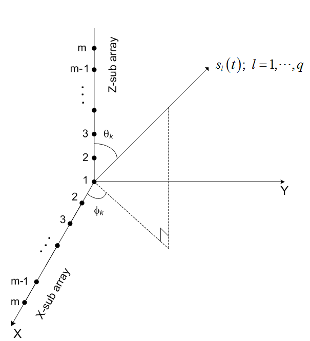
Refer to caption
Figure 1: The L-shaped array configuration

The gain of an element at a position (x,y,z)(x,y,z) for a signal with reference to origin from the direction (θ,ϕ)(\theta,\phi) is given by

a⁡(θ,ϕ)=ej⁡(2​π/λ)​(x​sin⁡θ​cos⁡ϕ+y​sin⁡θ​sin⁡ϕ+z​cos⁡θ)a(\theta,\phi)=e^{j(2\pi/\lambda)(x\sin{\theta}\cos{\phi}+y\sin{\theta}\sin{\phi}+z\cos{\theta})} (1)

Suppose that there are qq narrow band sources, with same wavelength λ\lambda impinging on each sensor. An llth source has an incidence angle θl\theta_{l} and an azimuth angle ϕl\phi_{l}, l=1,2,…,ql=1,2,...,q.

The signal received at the iith element of the Z-subarray is given by  [1]

zi​(t)=∑l=1qaz,i​(θl,ϕl)​sl​(t)+nz,i​(t)z_{i}(t)=\sum_{l=1}^{q}a_{z,i}(\theta_{l},\phi_{l})s_{l}(t)+n_{z,i}(t) (2)

where

az,i​(θl,ϕl)\displaystyle a_{z,i}(\theta_{l},\phi_{l}) =\displaystyle= ejβdcosθl\displaystyle e^{j\beta d\cos{\theta_{l}}}
=\displaystyle= ej2π(i−1)(d/λ)cosθl\displaystyle e^{j2\pi(i-1)(d/\lambda)\cos{\theta_{l}}}
=\displaystyle= ej⁡(i−1)​ψl\displaystyle e^{j(i-1)\psi_{l}}
ψl=2π(d/λ)cosθl\psi_{l}=2\pi(d/\lambda)\cos{\theta_{l}} (3)

sl​(t)s_{l}(t) is the complex envelope of the llth signal arriving from the direction (θl,ϕl)(\theta_{l},\phi_{l})
and nz,i​(t)n_{z,i}(t) is the zero-mean additive white Gaussian noise (AWGN) whose properties are mentioned in Section 2.2.

The signal received at the iith element of the X-subarray is given by

xi​(t)=∑l=1qax,i​(θl,ϕl)​sl​(t)+nx,i​(t)x_{i}(t)=\sum_{l=1}^{q}a_{x,i}(\theta_{l},\phi_{l})s_{l}(t)+n_{x,i}(t) (4)

where

ax,i​(θl,ϕl)\displaystyle a_{x,i}(\theta_{l},\phi_{l}) =\displaystyle= ej2π(i−1)(d/λ)sinθlcosϕl\displaystyle e^{j2\pi(i-1)(d/\lambda)\sin{\theta_{l}}\cos{\phi_{l}}}
=\displaystyle= ej⁡(i−1)​ξl,\displaystyle e^{j(i-1)\xi_{l}},
ξl=2π(d/λ)sinθlcosϕl\xi_{l}=2\pi(d/\lambda)\sin{\theta_{l}}\cos{\phi_{l}} (5)

and nx,i​(t)n_{x,i}(t) is the zero-mean AWGN.

If we collect outputs of all the sensors on the Z-subarray into an m×1m\times 1 vector, we have

𝐳⁡(t)=∑l=1q𝐚z​(θl,ϕl)​sl​(t)+𝐧z​(t)\mathbf{z}(t)=\sum_{l=1}^{q}\mathbf{a}_{z}(\theta_{l},\phi_{l})s_{l}(t)+\mathbf{n}_{z}(t) (6)

where

𝐳(t)=[z1(t)z2(t)⋯zm(t)]T\mathbf{z}(t)=[z_{1}(t)\hskip 14.45377ptz_{2}(t)\hskip 7.22743pt\cdots\hskip 7.22743ptz_{m}(t)]^{T}

𝐚z​(θl,ϕl)\mathbf{a}_{z}(\theta_{l},\phi_{l})   is the m×1m\times 1 steering vector of the Z-subarray towards the direction (θl,ϕl)(\theta_{l},\phi_{l}) given by

𝐚z(θl,ϕl)=[az,1(θl,ϕlaz,2(θl,ϕl)⋯az,m(θl,ϕl)]T\mathbf{a}_{z}(\theta_{l},\phi_{l})=[a_{z,1}(\theta_{l},\phi_{l}\hskip 14.45377pta_{z,2}(\theta_{l},\phi_{l})\hskip 7.22743pt\cdots\hskip 7.22743pta_{z,m}(\theta_{l},\phi_{l})]^{T}

and

𝐧z​(t)=[nz,1​(t)nz,2​(t)⋯nz,m​(t)]T\mathbf{n}_{z}(t)=\left[\begin{array}[]{cccc}n_{z,1}(t)&n_{z,2}(t)&\cdots&n_{z,m}(t)\end{array}\right]^{T}

We can rewrite (6) as

𝐳⁡(t)=(az,1​(θ1,ϕ1)az,1​(θ2,ϕ2)⋯az,1​(θq,ϕq)az,2​(θ1,ϕ1)az,2​(θ2,ϕ2)⋯az,2​(θq,ϕq)⋮⋮⋮⋮az,m​(θ1,ϕ1)az,m​(θ2,ϕ2)⋯az,m​(θq,ϕq))​(s1​(t)s2​(t)⋮sq​(t))+(nz,1​(t)nz,2​(t)⋮nz,m​(t))\small{\mathbf{z}(t)=\left(\begin{array}[]{cccc}a_{z,1}(\theta_{1},\phi_{1})&a_{z,1}(\theta_{2},\phi_{2})&\cdots&a_{z,1}(\theta_{q},\phi_{q})\\ a_{z,2}(\theta_{1},\phi_{1})&a_{z,2}(\theta_{2},\phi_{2})&\cdots&a_{z,2}(\theta_{q},\phi_{q})\\ \vdots&\vdots&\vdots&\vdots\\ a_{z,m}(\theta_{1},\phi_{1})&a_{z,m}(\theta_{2},\phi_{2})&\cdots&a_{z,m}(\theta_{q},\phi_{q})\end{array}\right)\left(\begin{array}[]{c}s_{1}(t)\\ s_{2}(t)\\ \vdots\\ s_{q}(t)\end{array}\right)+\left(\begin{array}[]{c}n_{z,1}(t)\\ n_{z,2}(t)\\ \vdots\\ n_{z,m}(t)\end{array}\right)} (7)

Similarly for the X-subarray, we have

𝐱⁡(t)=∑l=1q𝐚x​(θl,ϕl)​sl​(t)+𝐧x​(t)\mathbf{x}(t)=\sum_{l=1}^{q}\mathbf{a}_{x}(\theta_{l},\phi_{l})s_{l}(t)+\mathbf{n}_{x}(t) (8)

where

𝐱(t)=[x1(t)x2(t)⋯xm(t)]T\mathbf{x}(t)=[x_{1}(t)\hskip 14.45377ptx_{2}(t)\hskip 7.22743pt\cdots\hskip 7.22743ptx_{m}(t)]^{T}
𝐚x(θl,ϕl)=[ax,1(θl,ϕlax,2(θl,ϕl)⋯ax,m(θl,ϕl)]T\mathbf{a}_{x}(\theta_{l},\phi_{l})=[a_{x,1}(\theta_{l},\phi_{l}\hskip 14.45377pta_{x,2}(\theta_{l},\phi_{l})\hskip 7.22743pt\cdots\hskip 7.22743pta_{x,m}(\theta_{l},\phi_{l})]^{T}

and

𝐧x(t)=[nx,1(t)nx,2(t)⋯nx,m(t)]T\mathbf{n}_{x}(t)=[n_{x,1}(t)\hskip 14.45377ptn_{x,2}(t)\hskip 7.22743pt\cdots\hskip 7.22743ptn_{x,m}(t)]^{T}

Note that (8) can be rewritten as

𝐱⁡(t)=(ax,1​(θ1,ϕ1)ax,1​(θ2,ϕ2)⋯ax,1​(θq,ϕq)ax,2​(θ1,ϕ1)ax,2​(θ2,ϕ2)⋯ax,2​(θq,ϕq)⋮⋮⋮⋮ax,m​(θ1,ϕ1)ax,m​(θ2,ϕ2)⋯ax,m​(θq,ϕq))​(s1​(t)s2​(t)⋮sq​(t))+(nx,1​(t)nx,2​(t)⋮nx,m​(t))\small{\mathbf{x}(t)=\left(\begin{array}[]{cccc}a_{x,1}(\theta_{1},\phi_{1})&a_{x,1}(\theta_{2},\phi_{2})&\cdots&a_{x,1}(\theta_{q},\phi_{q})\\ a_{x,2}(\theta_{1},\phi_{1})&a_{x,2}(\theta_{2},\phi_{2})&\cdots&a_{x,2}(\theta_{q},\phi_{q})\\ \vdots&\vdots&\vdots&\vdots\\ a_{x,m}(\theta_{1},\phi_{1})&a_{x,m}(\theta_{2},\phi_{2})&\cdots&a_{x,m}(\theta_{q},\phi_{q})\end{array}\right)\left(\begin{array}[]{c}s_{1}(t)\\ s_{2}(t)\\ \vdots\\ s_{q}(t)\end{array}\right)+\left(\begin{array}[]{c}n_{x,1}(t)\\ n_{x,2}(t)\\ \vdots\\ n_{x,m}(t)\end{array}\right)} (9)

2 Proposed Method

Consider the Z-subarray:

On substituting the values of az,i​(θl,ϕl)a_{z,i}(\theta_{l},\phi_{l}) in (7) for i=1,2,…,mi=1,2,...,m and l=1,2,..,ql=1,2,..,q , we have

𝐳⁡(t)=(11⋯1ej​ψ1ej​ψ2⋯ej​ψ​q⋮⋮⋮⋮ej⁡(m−1)​ψ1ej⁡(m−1)​ψ2⋯ej⁡(m−1)​ψq)​(s1​(t)s2​(t)⋮sq​(t))+(nz,1​(t)nz,2​(t)⋮nz,m​(t))\mathbf{z}(t)=\left(\begin{array}[]{cccc}1&1&\cdots&1\\ e^{j\psi_{1}}&e^{j\psi_{2}}&\cdots&e^{j\psi{q}}\\ \vdots&\vdots&\vdots&\vdots\\ e^{j(m-1)\psi_{1}}&e^{j(m-1)\psi_{2}}&\cdots&e^{j(m-1)\psi_{q}}\end{array}\right)\left(\begin{array}[]{c}s_{1}(t)\\ s_{2}(t)\\ \vdots\\ s_{q}(t)\end{array}\right)+\left(\begin{array}[]{c}n_{z,1}(t)\\ n_{z,2}(t)\\ \vdots\\ n_{z,m}(t)\end{array}\right) (10)

where {ψl}\{\psi_{l}\} are defined in (3).

By collecting MM equispaced snapshots from each sensor, a data matrix Z is formed as follows

Z=(11⋯1ej​ψ1ej​ψ2⋯ej​ψq⋮⋮⋮⋮ej⁡(m−1)​ψ1ej⁡(m−1)​ψ2⋯ej⁡(m−1)​ψq)​(s1​(t1)s1​(t2)⋯s1​(tM)s2​(t1)s2​(t2)⋯s2​(tM)⋮⋮⋮⋮sq​(t1)sq​(t2)⋯sq​(tM))+(nz,1​(t1)nz,1​(t2)⋯nz,1​(tM)nz,2​(t1)nz,2​(t2)⋯nz,2​(tM)⋮⋮⋮⋮nz,m​(t1)nz,m​(t2)⋯nz,m​(tM))\begin{split}Z=\left(\begin{array}[]{cccc}1&1&\cdots&1\\ e^{j\psi_{1}}&e^{j\psi_{2}}&\cdots&e^{j\psi_{q}}\\ \vdots&\vdots&\vdots&\vdots\\ e^{j(m-1)\psi_{1}}&e^{j(m-1)\psi_{2}}&\cdots&e^{j(m-1)\psi_{q}}\end{array}\right)\left(\begin{array}[]{cccc}s_{1}(t_{1})&s_{1}(t_{2})&\cdots&s_{1}(t_{M})\\ s_{2}(t_{1})&s_{2}(t_{2})&\cdots&s_{2}(t_{M})\\ \vdots&\vdots&\vdots&\vdots\\ s_{q}(t_{1})&s_{q}(t_{2})&\cdots&s_{q}(t_{M})\\ \end{array}\right)&\\ \\ +\left(\begin{array}[]{cccc}n_{z,1}(t_{1})&n_{z,1}(t_{2})&\cdots&n_{z,1}(t_{M})\\ n_{z,2}(t_{1})&n_{z,2}(t_{2})&\cdots&n_{z,2}(t_{M})\\ \vdots&\vdots&\vdots&\vdots\\ n_{z,m}(t_{1})&n_{z,m}(t_{2})&\cdots&n_{z,m}(t_{M})\\ \end{array}\right)&\end{split} (11)

or

Z=Az​S+NzZ=A_{z}S+N_{z} (12)

where

Z=(z1​(t1)z1​(t2)⋯z1​(tM)z2​(t1)z2​(t2)⋯z2​(tM)⋮⋮⋮⋮zm​(t1)zm​(t2)⋯zm​(tM))Z=\left(\begin{array}[]{cccc}z_{1}(t_{1})&z_{1}(t_{2})&\cdots&z_{1}(t_{M})\\ z_{2}(t_{1})&z_{2}(t_{2})&\cdots&z_{2}(t_{M})\\ \vdots&\vdots&\vdots&\vdots\\ z_{m}(t_{1})&z_{m}(t_{2})&\cdots&z_{m}(t_{M})\\ \end{array}\right)

The matrices AzA_{z} and SS are unknown, and are not rank-deficient by assumption.

Now, let y1=ej​ψ1y_{1}=e^{j\psi_{1}}, y2=ej​ψ2y_{2}=e^{j\psi_{2}},…, yq=ej​ψqy_{q}=e^{j\psi_{q}} and assume that y1,y2,…,yqy_{1},y_{2},...,y_{q} are the roots of a polynomial equation

𝒫⁡(y)=1+c1​y+c2​y2+⋯+cm−1​ym−1=0.{\cal{P}}(y)=1+c_{1}y+c_{2}y^{2}+\cdots+c_{m-1}y^{m-1}=0. (13)

Now our aim is to calculate the coefficients which satisfy this assumption and then to solve for the roots.

2.1 Method without Noise

From (13) and (11), it can easily be shown that the following equations hold for no noise case.

z1​(t1)+c1​z2​(t1)+c2​z3​(t1)+⋯+cm−1​zm​(t1)\displaystyle z_{1}(t_{1})+c_{1}z_{2}(t_{1})+c_{2}z_{3}(t_{1})+\cdots+c_{m-1}z_{m}(t_{1}) =\displaystyle= 0\displaystyle 0
z1​(t2)+c1​z2​(t2)+c2​z3​(t2)+⋯+cm−1​zm​(t2)\displaystyle z_{1}(t_{2})+c_{1}z_{2}(t_{2})+c_{2}z_{3}(t_{2})+\cdots+c_{m-1}z_{m}(t_{2}) =\displaystyle= 0\displaystyle 0
⋮\displaystyle\vdots\hskip 144.54pt
z1​(tM)+c1​z2​(tM)+c2​z3​(tM)+⋯+cm−1​zm​(tM)\displaystyle z_{1}(t_{M})+c_{1}z_{2}(t_{M})+c_{2}z_{3}(t_{M})+\cdots+c_{m-1}z_{m}(t_{M}) =\displaystyle= 0\displaystyle 0

After simple manipulations,

c1​z2​(t1)+c2​z3​(t1)+⋯+cm−1​zm​(t1)\displaystyle c_{1}z_{2}(t_{1})+c_{2}z_{3}(t_{1})+\cdots+c_{m-1}z_{m}(t_{1}) =\displaystyle= −z1​(t1)\displaystyle-z_{1}(t_{1})
c1​z2​(t2)+c2​z3​(t2)+⋯+cm−1​zm​(t2)\displaystyle c_{1}z_{2}(t_{2})+c_{2}z_{3}(t_{2})+\cdots+c_{m-1}z_{m}(t_{2}) =\displaystyle= −z1​(t2)\displaystyle-z_{1}(t_{2})
⋮\displaystyle\vdots\hskip 144.54pt
c1​z2​(tM)+c2​z3​(tM)+⋯+cm−1​zm​(tM)\displaystyle c_{1}z_{2}(t_{M})+c_{2}z_{3}(t_{M})+\cdots+c_{m-1}z_{m}(t_{M}) =\displaystyle= −z1​(tM)\displaystyle-z_{1}(t_{M})

The above set of equations can be written in matrix form as

(z2​(t1)z3​(t1)⋯zm​(t1)z2​(t2)z3​(t2)⋯zm​(t2)⋮⋮z2​(tM)z3​(tM)⋯zm​(tM))​(c1c2⋮cm−1)=(−z1​(t1)−z1​(t2)⋮−z1​(tM))\left(\begin{array}[]{cccc}z_{2}(t_{1})&z_{3}(t_{1})&\cdots&z_{m}(t_{1})\\ z_{2}(t_{2})&z_{3}(t_{2})&\cdots&z_{m}(t_{2})\\ &\vdots&&\vdots\\ z_{2}(t_{M})&z_{3}(t_{M})&\cdots&z_{m}(t_{M})\end{array}\right)\left(\begin{array}[]{c}c_{1}\\ c_{2}\\ \vdots\\ c_{m-1}\end{array}\right)=\left(\begin{array}[]{c}-z_{1}(t_{1})\\ -z_{1}(t_{2})\\ \vdots\\ -z_{1}(t_{M})\end{array}\right) (14)

or

P​C=P1PC=P_{1} (15)

This is an overdetermined system of equations. The best solution in the least square sense for the coefficient vector C is given by

C=P#​P1C=P^{\#}P_{1} (16)

where P#P^{\#} is the Moore-Penrose pseudoinverse of PP,

P#=(PH​P)−1​PHP^{\#}=(P^{H}P)^{-1}P^{H}

Substitute c1,c2,…,cm−1c_{1},c_{2},\ldots,c_{m-1} obtained in (16) into (13) and solve for the roots of 𝒫⁡(y){\cal{P}}(y). There are (m−1)(m-1) roots, and among those only q solutions are of our interest. From the (m−1)(m-1) roots choose qq roots say {γl\gamma_{l}}, whose magnitudes are nearer to unity:

γl=ej2π(d/λ)cosθll=1,2,…,q\gamma_{l}=e^{j2\pi(d/\lambda)\cos{\theta_{l}}}\hskip 50.58878ptl=1,2,\ldots,q (17)

Then, the estimate of ψl\psi_{l} is

ψl^=a​n​g​l​e​{γl}\hat{\psi_{l}}=angle\{\gamma_{l}\} (18)

Follow the similar approach for the X-subarray to calculate {βl\beta_{l}} defined by

βl=ej2π(d/λ)sinθlcosϕll=1,2,…,q\beta_{l}=e^{j2\pi(d/\lambda)\sin{\theta_{l}\cos{\phi_{l}}}}\hskip 50.58878ptl=1,2,\ldots,q (19)

and hence

ξl^=a​n​g​l​e​{βl}\hat{\xi_{l}}=angle\{\beta_{l}\}\hskip 72.26999pt (20)

Now the estimates of θl\theta_{l} and ϕl\phi_{l} are given by

θl^=sin−1⁡(ψ^l2​π​(d/λ))l=1,2,…,q.\hat{\theta_{l}}=\sin^{-1}{\left(\frac{\hat{\psi}_{l}}{2\pi(d/\lambda)}\right)}\hskip 72.26999ptl=1,2,\ldots,q. (21)
ϕl^=cos−1⁡(ξ^l(2π(d/λ)sinθ^l))l=1,2,…,q.\hat{\phi_{l}}=\cos^{-1}{\left(\frac{\hat{\xi}_{l}}{(2\pi(d/\lambda)\sin{\hat{\theta}_{l}})}\right)}\hskip 65.04256ptl=1,2,\ldots,q. (22)

2.2 Method with Noise

Note that in (6) and (8), the vectors 𝐧z​(t)\mathbf{n}_{z}(t) and 𝐧x​(t)\mathbf{n}_{x}(t) are random noise components on Z and X subarrays respectively. The noise is assumed to be additive, temporally white Gaussian with zero mean. This assumption is a valid assumption in real-world applications.

Mathematically, we can express the above stated properties of the noise as follows,

E⁡[𝐧z​(t)]=E⁡[𝐧x​(t)]=𝟎E[\mathbf{n}_{z}(t)]=E[\mathbf{n}_{x}(t)]=\mathbf{0} (23)
E⁡[𝐧z​(t)​𝐧zH​(t)]=E⁡[𝐧x​(t)​𝐧xH​(t)]=σ2​𝐈E[\mathbf{n}_{z}(t)\mathbf{n}_{z}^{H}(t)]=E[\mathbf{n}_{x}(t)\mathbf{n}_{x}^{H}(t)]=\sigma^{2}\mathbf{I} (24)
E⁡[𝐧z​(t)​𝐧zT​(t)]=E⁡[𝐧x​(t)​𝐧xT​(t)]=𝟎E[\mathbf{n}_{z}(t)\mathbf{n}_{z}^{T}(t)]=E[\mathbf{n}_{x}(t)\mathbf{n}_{x}^{T}(t)]=\mathbf{0} (25)

and

E⁡[𝐧z​(ti)​𝐧zH​(tj)]=E⁡[𝐧z​(ti)​𝐧zT​(tj)]=𝟎for ​i≠jE[\mathbf{n}_{z}(t_{i})\mathbf{n}_{z}^{H}(t_{j})]=E[\mathbf{n}_{z}(t_{i})\mathbf{n}_{z}^{T}(t_{j})]=\mathbf{0}\hskip 36.135pt\text{for }i\neq j (26)
E⁡[𝐧x​(ti)​𝐧xH​(tj)]=E⁡[𝐧x​(ti)​𝐧xT​(tj)]=𝟎for ​i≠jE[\mathbf{n}_{x}(t_{i})\mathbf{n}_{x}^{H}(t_{j})]=E[\mathbf{n}_{x}(t_{i})\mathbf{n}_{x}^{T}(t_{j})]=\mathbf{0}\hskip 36.135pt\text{for }i\neq j (27)

where EE denotes the expectation operation, H denotes the Hermitian operation, T denotes the transposition, and tit_{i} and tjt_{j} are the iith and jjth time instants respectively.

The noise has an negative impact on the accuracy of estimates of the polynomial coefficients. In order to reduce the effect of the noise, we follow the same procedure except for the calculation of inverse of the matrix PP in (15) where we use the singular value decomposition(SVD) as discussed below.
Let the SVD of PP be

P=U​Σ​VHP=U\Sigma V^{H} (28)

where UU and VV are the unitary matrices containing the singular vectors of P and Σ\Sigma is a diagonal matrix of same dimensions as PP, and it is given by

Σ=UH​P​V\Sigma=U^{H}PV (29)

The diagonal elements in Σ\Sigma are non-negative and are sorted in decreasing order, i.e.,

Σ=d​i​a​g​{τ1,τ2,…,τq,…,τm−1}\Sigma=diag\{\tau_{1},\tau_{2},\ldots,\tau_{q},\ldots,\tau_{m-1}\} (30)

where

τ1≥τ2≥⋯≥τq≥⋯≥τm−1\tau_{1}\geq\tau_{2}\geq\cdots\geq\tau_{q}\geq\cdots\geq\tau_{m-1}

are the singular values of PP.

To reduce the effect of noise, replace the last m−q−1m-q-1 singular values with zero in calculating the inverse of PP, i.e.,

Σ1=d​i​a​g​{τ1,τ2,…,τq,0,…}\Sigma_{1}=diag\{\tau_{1},\tau_{2},\ldots,\tau_{q},0,\ldots\} (31)

and

Σ1−1=d​i​a​g​{1/τ1,1/τ2,…,1/τq,0,…}\Sigma_{1}^{-1}=diag\{1/\tau_{1},1/\tau_{2},\ldots,1/\tau_{q},0,\ldots\} (32)

The dimensions of Σ1−1\Sigma_{1}^{-1} are same as that of PHP^{H}.
The lease squares approximation of P−1P^{-1} is given by  [3]

P−1=V​Σ1−1​UHP^{-1}=V\Sigma_{1}^{-1}U^{H} (33)

hence, the estimate of coefficient vector in (15) is

C=V​Σ1−1​UH​P1C=V\Sigma_{1}^{-1}U^{H}P_{1} (34)

Follow the same approach for X-subarray to obtain the coefficient vector and the roots. The computation of AOAs from the roots is same as that for the noiseless case.

References

  • [1] N. Tayem and H. M. Kwon, “L-shape 2-dimensional arrival angle estimation with propagator method,” IEEE Trans. Antennas and Propagation, vol. 53, no. 5, pp. 1622–1630, May 2005.
  • [2] P. Singh and P. Sircar, “Time delays and angles of arrival estimation using known signals”, Signal, Image and Video Processing, vol. 6, no. 2, pp. 171–178, Feb. 2011.
  • [3] P. Dewilde and E. F. Deprettere, “Singular value decomposition: An introduction,” In E. F. Deprettere (ed.), SVD and Signal Processing: Algorithms, Applications, and Architectures, pp. 3–41. Elsevier Science, North Holland, 1988.