Sharp uncertainty relations for number and angle
Abstract
We study uncertainty relations for pairs of conjugate variables like number and angle, of which one takes integer values and the other takes values on the unit circle. The translation symmetry of the problem in either variable implies that measurement uncertainty and preparation uncertainty coincide quantitatively, and the bounds depend only on the choice of two metrics used to quantify the difference of number and angle outputs, respectively. For each type of observable we discuss two natural choices of metric, and discuss the resulting optimal bounds with both numerical and analytic methods. We also develop some simple and explicit (albeit not sharp) lower bounds, using an apparently new method for obtaining certified lower bounds to ground state problems.
I Introduction
The study of uncertainty relations has experienced a major boost in recent years. As more and more experiments reach quantum limited accuracy, sharp quantitative uncertainty and error bounds become more relevant. It has also become evident that the subject of quantum uncertainty cannot be reduced to the classic standard uncertainty relation that was first made rigorous by Kennard [1], Robertson [2] and others and is now found in every textbook. The purpose of this paper is to present a new case study that exemplifies the three main directions of generalization currently being pursued. The example at hand is given by the number-angle pair of observables, where by “number” we understand an observable whose spectrum is the set of all integers.
The first extension of the uncertainty principle concerns the set of scenarios to which quantitative uncertainty relations apply. The Kennard relation is a “preparation uncertainty relation”, i.e., a quantitative expression of the observation that there is no state preparation for which the distributions of two observables under consideration are both sharp. This relation can be tested, in principle, by separate runs of precise measurements of the two observables, performed on ensembles of systems in the same state. In contrast to this, one may consider attempted joint measurements of noncommuting observables, as already intuitively envisaged by Heisenberg [3]; one finds that such joint measurements are constrained by “measurement uncertainty relations” [4, 5, 6] which describe the unavoidable error bounds.
The number-angle pair also highlights the need to consider uncertainty measures other than standard deviations. The second direction of generalization to be considered is thus in the concrete mathematical expressions measuring the “sharpness” of distributions, or the error of an approximate measurement. We will consider two alternative types of uncertainty measures and associated error measures for each of the two observables concerned.
Finally, the third direction of generalization concerns the forms of preparation and measurement uncertainty relations that are applicable to arbitrary pairs of observables. The Robertson relation involving the expectations of the commutator in the lower bound fails to provide preparation uncertainty relation in the above sense because the only state-independent lower bound one can get from it is zero. Nevertheless, non-trivial state-independent bounds usually do exist. Uncertainty is really a ubiquitous phenomenon, joint measurability or simultaneous sharp preparability are the exceptions rather than the rule. Accordingly, the problem of establishing tight uncertainty relations for pairs of observables amounts to the task of establishing their (preparation or measurement) uncertainty regions, defined as the set of pairs of uncertainty values in all states (for preparation uncertainty) and the set of pairs of error values in all possible joint measurements (for measurement uncertainty), respectively.
It is a pleasing property of the case at hand—number and angle—that an essentially complete treatment can be given. This is due to the phase space symmetry which implies, exactly as for standard position and momentum [7], that “metric distance” and “calibration distance” for the error assessment of observables satisfy the same relations and also that they are quantitatively the same as corresponding preparation uncertainty relations. In this paper we deduce the ensuing measurement uncertainty relations for number and angle.
Our paper is organized according to the methods employed. In Section II we review the conceptualization of the preparation uncertainty measures and associated error measures to be used throughout the paper. This is followed by an overview of our main results (Section III). In Section IV we show how the phase space symmetry can be exploited to find optimal joint measurements among the covariant phase space observables. Here we show the identity of preparation uncertainty regions and measurement uncertainty (or error) regions in the case at hand, introducing calibration uncertainty regions as a mediating construct. The lower boundary of the uncertainty regions is characterized as a ground state problem. Numerical estimates of the optimal tradeoff curves are shown in Section V. Next, Sections VI and VII give determinations of the exact ground states and lower boundaries for the various combinations of deviation measures, and we show how existing uncertainty relations for number and phase can be reproduced or strengthened using our systematic approach. We conclude with an outlook in Section VIII.
II Conceptual Uncertainty Basics
II.1 Number and angle observables
The complementarity between number and angle appears in physics in various guises. Essentially, this is for any parameter with a natural periodicity. Geometric angles are one case, with the complementary variable given by a component of angular momentum. Another important case is quantum optical phase, which is complementary to an harmonic oscillator Hamiltonian. At least for preparation uncertainty this is no difficulty, since a relation valid for all states also holds for states supported on the subspace of positive integers. One does get additional or sharper relations from building in this constraint, however. A further important field of applications is quasi-momentum with values in the Brillouin-Zone for a lattice system (of which we only consider the one-dimensional case here). This is also related to form factors arising in the discussion of diffraction patterns and fringe contrast from periodic gratings [8].
The literature on angle-angular momentum uncertainty is almost exclusively concerned with the preparation scenario, although the lack of an error disturbance relation has been noted [9]. In the preparation case a major obstacle was the Kennard and Robertson [2] relation and their role as a model how uncertainty relations should be set up. There is nothing wrong with an observable with outcomes on a circle. But much work was wasted on the question of how to represent “angle” measurements by a selfadjoint operator [10, 11]. Additional unnecessary confusion in the case of semibounded number and quantum optical phase was generated by the ignorance or lack of acceptance of generalized (“POVM”) observables. On the positive side, an influential paper by Judge [12] produced a relation (for the arc metric), and conjectured an improvement, which was proved shortly afterwards [13]. In this context the role of ground state problems for finding optimal bounds, which is also the basis of our methods, seems to have appeared for the first time [14]. The appearance of the chordal metric grew out of the approach of avoiding the “angle” problem, replacing by the two selfadjoint operators and .
II.2 Measures of uncertainty and error
Both in preparation and in measurement uncertainty we have to assess the difference of probability distributions: For preparation uncertainty it is the difference from a sharp distribution concentrated on a single point. This is also the basis of calibration error assessment. For metric error we also need to express the distance of two general distributions. We want to express the distance between distributions on the same scale as the distance of points. For example, in the case of position and momentum errors, for all error measures one considers to be measured in length units and in momentum units, and this is satisfied by the choice of standard deviation for these measures.
So let us assume that the outcomes of some observable (represented by a POVM, a positive operator valued measure) lie in a space with metric . For real valued quantities like a single component of position or momentum this usually means and .
We now extend the distance function on the points to a distance between a probability measure on and a point . It will just the be the mean distance from :
| (1) |
Here the exponent gives some extra flexibility as to how large deviations are weighted relative to small ones. The root ensures that the result is still in the same units as , and also that for a point measure concentrated on a point we have for all . It is also true for all that happens only for the point measure at . We will later mostly choose and drop the index ; in this case is the root mean square distance from for points distributed according to .
With this measure of deviation of a distribution from the point we can introduce the generalized standard deviation,
| (2) |
Note that for , and this recovers exactly the usual standard deviation, with the minimum being attained at the mean of . The symbol is just a reminder of the minimization, and emphasizes that is just the distance of from the set of point measures.
For this interpretation to make sense we must also let the second argument of be a general probability distribution , resulting in a metric on the set of probability measures. The canonical definition here is the transport distance [15]
| (3) |
where “” is a shorthand for , the variable in this infimum, being a “coupling” of and , i.e., it is a measure on with and as its marginal distributions. One should think of as a plan for converting the distribution into , maybe for some substance rather than for probability. The cost of transferring a mass unit from to is supposed to be , and the plan records just how much mass is to be moved from to . The marginal property means that the initial distribution is and the final one . Then is the optimized cost. When the final distribution is a point measure, there is not much to plan, and we recover (1). Therefore there is little danger of confusion in using the same symbol for the metrics of points and of probability measures.
Now we can use these notions of spread and distance for expressing uncertainties related to observables with outcome spaces and , each with a suitably chosen metric and error exponent. Let us denote by the probability measure of outcomes in upon measuring on systems prepared according to . To express preparation uncertainty, let us consider the set PU of generalized variance pairs
| (4) |
A preparation uncertainty relation is some inequality saying that the uncertainty region does not extend to the origin: the two deviations cannot both be simultaneously small. If this set is known, we consider it as the most comprehensive expression of preparation uncertainty. Its description by inequalities for products or weighted sums or whatever other expression is a matter of mathematical convenience, and we will, of course, develop appropriate expressions. A lower bound for the product is useful only for position and momentum and its mathematical equivalents. In this case the dilatation invariance forces the uncertainty region to be bounded by an exact hyperbola. But if one of the observables considered can take discrete values, the set will reach an axis, making every state-independent lower bound on the product trivial.
We should note that the set (4) is in general not convex, and can have holes (for examples, see [16]). However, in order to express lower bounds, the essence of uncertainty, it makes no difference if we fill in these holes, and include with every point also those for which both coordinates are larger or the same. The resulting set, the ‘monotone hull’ of PU, is bounded below by the graph of a non-increasing function, the tradeoff curve (see Fig. 1 for examples). It still need not be convex in general, but we will see that convexity holds in the examples we study.
For measurement uncertainty we again consider two observables (POVMs) with the same outcomes, metrics and error exponents. Now the question is: can be measured jointly? The claim is, usually, that no matter how we try there will be an error in our implementation. So let be the margins of some joint measurement with outcomes . Then must exhibit some errors relative to , i.e., some output distributions must be different from . We define as the error of with respect to the quantity
| (5) |
Note that we are using here a worst case quantity with respect to the input state. This is what we should do for a figure of merit for a measuring instrument. If a manufacturer claims that his device will produce distributions -close to those of for any input state, he is saying that . Making such a claim for just a single state is as useless as advertising a clock which measures “the time ” very precisely (but maybe no other). Now we can look at the uncertainty region
| (6) |
where the notation indicates that and are jointly measurable (that is, they are margins of some POVM that serves as a joint observable). All general remarks made about the preparation uncertainty region PU also hold for MU.
The supremum in (5) is rather demanding experimentally. Good practice for testing the quality of a measuring device is calibration, i.e., testing it on states with known properties, and seeing whether the device reproduces these properties. In our case this means testing the device on states whose -distribution is sharply concentrated around some , and looking at the spread of the -distribution around the same . We define as the calibration error of with respect to the quantity
| (7) |
Here the limit exists because the set (and hence the sup) is decreasing as . This definition only makes sense if there actually are sufficiently many sharp states for , so we will use this definition only when the reference observable is projection valued. Since the calibration states in this definition are also contained in the supremum (5), it is clear that , so the set CU of calibration error pairs will generally be larger than MU.
III Setting and Overview of Results
We now consider systems with Hilbert space , where denotes the unit circle, with the integration over angle. The notation derives from “torus” and is customary in group theory. We use it here to emphasize the group structure (of multiplying phases or adding angles mod ) but also to avoid a fixed coordinatization such as , which would misleadingly assign a special role to the cut point . We will refer to as our “position space”. The corresponding “momentum” space is , and changing to the momentum representation in is done by the unitary operator of expanding in a Fourier series. With denoting the Fourier basis, this means that
| (8) |
We have two natural projection valued observables, the angle (=position, phase) observable taking values on , and the number (=angular momentum observable) with values in . That is, if is some function of the angle variable, denotes the multiplication operator , and similarly denotes the multiplication by a function in the momentum representation. The outcome proability densities of these observables on an input state are denoted by and , respectively. Thus,
| (9) | |||||
| (10) |
Then the basic claim of preparation uncertainty is that and cannot be simultaneously sharp, and the basic claim of measurement uncertainty is that there is is no observable with pairs of outcomes for which the marginal distributions found on input state are close to and .
In order to apply the ideas of the previous section, we need to choose a metric in each of these spaces. For discrete values () we can naturally take the standard distance or a discrete metric:
| (11) |
Similarly, there are two natural choices for angles, depending on whether the basis for the comparison is how far we have to rotate to go from to (“arc distance”) or else the distance of phase factors and in the plane (“chordal distance”):
| (12) |
The variances based on these bounded metrics will have an upper bound. Since the minimum in (2) makes a concave function of , so that we find, by averaging over translates, that the equidistribution has the maximal variance for all translation invariant metrics and all exponents. Both metrics, or rather their quadratic () variances have been discussed before. The -variance was used by Lévy [17] and Judge [12], the -variance seems to have appeared first in von Mises [18]. In fact, the quadratic chordal variance can also be written as
| (13) | |||||
which is von Mises’ “circular variance”. For a review of these choices see Ref. 19. The only property needed in our approach is that the metric should not break the rotation invariance, i.e., it should be a function of the difference of angles. We will therefore use every metric also as a single variable function, i.e., and . Functions which do not come from a metric have been considered in Ref. 20.
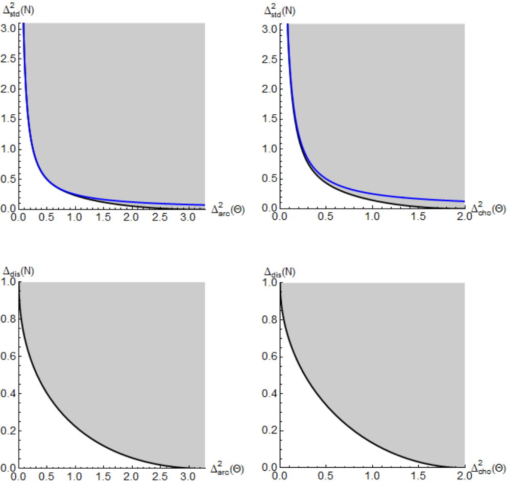
Then we have the following result.
Proposition 1.
For all error exponents and choices of translation invariant metric the three uncertainty regions coincide. They are depicted for in Figure 1. Every point on one of the tradeoff curves belongs to a unique pure state (resp. a unique extremal phase space covariant joint measurement).
The proof of this Proposition is based entirely on the corresponding proof for standard position and momentum [7]. We will sketch the main steps in the next section, and also show how the computation of the tradeoff curve can be reduced to solving ground state problems for certain Hamiltonians. The detailed features of these diagrams are then developed in the subsequent sections, sorted by the methods employed. The tradeoff curves in Figure 1 for the generalized variances, denoted simply , are determined numerically (see Section V). Since the algorithms employed provide optimal bounds, the figures are correct within pixel accuracy (which can be easily pushed to high accuracy). In fact, the problem is very stable, in the sense that near minimal uncertainty implies that the state (or joint observable) is close to the minimizing one. The bounds for this are in terms of the spectral gap of the Hamiltonian and are also discussed in Section V.
However, the only case in which the exact tradeoff curves can be described in closed form is (see Section VI.2)
| (14) |
even though, in all cases, the optimizing states can be expressed explicitly in terms of standard special functions (see Section VI). Therefore simple and explicit lower bounds are of interest. A problem here is that computing the variances for some particular state always produces a point inside the shaded area, i.e., an upper bound to the lower bound represented by the tradeoff curve. This is useless for applications, so in Section VII we develop a procedure proving lower bounds, and thus correct (if suboptimal) uncertainty relations.
IV Phase Space Symmetry and Reduction to a Ground State Problem
In this section we briefly sketch the arguments leading to the equality of preparation und measurement uncertainty regions. The full proof is directly parallel to the one given in Ref. 7 for position and momentum. The basic reference for phase space quantum mechanics is Ref. 21. The theory there is developed for phase spaces of the form , but all results we need here immediately carry over to the general case , where is a locally compact abelian group and is its dual, in our case and . A systematic extension of Ref. 21 to the general case, including the finer points, is in preparation in collaboration with Jussi Schultz.
IV.1 Covariant phase space observables
The phase space in our setting is the group . We join the position translations and the momentum translations to phase space translations, which are represented by the displacement or Weyl operators
| (15) |
These operators commute up to a phase, so that the operators , i.e., the action of the Weyl operators on bounded operators , is a representation of the abelian group . A crucial property is the square integrability of the matrix elements of the Weyl operators, which we will use in the form that for any two trace class operators on the formula
| (16) |
where . Hence, when both and are density operators the integrand in this equation is a probability density on . In summary [21]:
Proposition 2.
Every density operator serves an observable with outcomes in the phase space , via
| (17) |
Here figures as the operator valued Radon-Nikodym density with respect to of at the origin, and by translation also at arbitrary points. The observables obtained in this way are precisely the covariant ones, i.e., those satisfying the equation .
For the discussion of uncertainties we need the margins of such observables. One can guess their form from a fruitful classical analogy [21], by which the integrand in (16) can be read as a convolution of and . For classical probability densities on a cartesian product it is easily checked that the margin of the convolution is the convolution of the margins. The same is true for operators, only that the margins of a density operator are the classical distributions and described above. If is a probability density on phase space we will also denote by and the respective margins on and . In particular, for the output distribution of the covariant observable , i.e., , One checks readily checks the marginal relations
| (18) | ||||
| (19) |
where “” means the convolution of probability densities on and . Since this is the operation associated with the sum of independent random variables we arrive at the following principle:
Corollary 1.
Both margins of a covariant phase space measurement can be simulated by first making the corresponding ideal measurement on the input state, and then adding some independent noise, which is also independent of the input state. The distribution of this noise is the corresponding margin of the density operator .
This principle is responsible for the remarkable equality of the preparation uncertainty region and the measurement uncertainty regions and . Indeed the added noise is what distinguishes the margins of an attempted joint measurement from an ideal measurement, and this has precisely the distribution relevant for preparation uncertainty for .
IV.2 MU and CU: Reduction to the covariant case
While this principle explains quite well what happens in the case of covariant observables , Proposition 1 makes no covariance assumption. The key for reducing the general case is the observation that our quality criteria in terms of do not single out a point in phase space. Thus, let be the set of observables whose angle margin is -close to the ideal observable, , and whose number margin satisfies ; then this set is closed under phase space shifts, i.e., is unchanged when we replace by where
| (20) |
Note that the fixed points of all these transformations are precisely the covariant observables. The second point to note is that the set is convex, because the worst case error of an average in a convex combination is smaller than the average of the worst case errors. It is also a compact set in a suitable weak topology. This is in contrast to the set of all observables: Since there are arbitrarily large shifts in , we can shift an observable to infinity such that the probabilities for all fixed finite regions go to zero. The weak limit of such observables would be zero or, in an alternative formulation, would acquire some weight on points at infinity (a compactification of ). For such a sequence, however, the errors would also diverge. It is shown in Ref. 7 that this suffices to ensure the compactness of . Then the Markov-Kakutani Fixed Point Theorem (Ref. 22, Thm. V.10.6) ensures that contains a common fixed point of all the transformations (20).
In summary:
Proposition 3.
For every joint observable on the phase space there is a covariant one for which the errors are at least as good.
Therefore for determining we can just assume the observable in question to be covariant, implying the very simple form of the margins described above. The argument for is the same.
IV.3 The post-processing Lemma:
We have noted that, in general, , because for calibration the worst case analysis is done over a much smaller set of states. Indeed, it is easy to construct examples of observable pairs where the inequality is strict. There is a general result, Ref. 16, Lemma 8, however, which implies equality. The condition is that arises from by classical, possibly stochastic post-processing. That is, we can simulate by first measuring , and then adding noise or, in other words, generating a random output by a process which may depend on the measured -value. The noise is described then by a transition probability kernel for turning the measured value into somewhere in the set . is thus a description of the noise, and its relevant size is given by the formula
| (21) |
Here the -essential supremum of a measurable function is the supremum of all such that the level set has non-zero measure with respect to . This is needed to ensure that enters this formula only for values that can actually occur as outputs of .
IV.4 The covariant case:
In the case at hand, the noise is independent of , i.e., is translation invariant and so is the metric. Therefore, the integral in (21) is simply independent of . Moreover, we know the distribution of the noise on each margin to be the respective margin of , so that the integral is just the -power deviation of the margin from zero. So we get, for any choice of exponents and translation invariant metrics on and :
| (22) |
and similarly for . Note that the last term here is not the variance , because the minimization over in (2) is missing. Indeed, if just had zero variance, i.e, it were a point measure at some point , we would get a constant shift of size between the distributions and , and this would be the errors on the left hand side. So for a fixed we can only say that the terms in (22) are . On the other hand, we are looking for optimal and these will be obtained by shifting in such a way that (22) is minimized. Hence, as far as uncertainty diagrams are concerned, we can replace the last term by the -deviation. This concludes the proof that the three uncertainty diagrams coincide.
IV.5 Minimizing the variances
We now describe the general method to find the tradeoff curve. The idea is to fix some negative slope in the diagram, and ask for the lowest straight line with that slope intersecting . That is, we look at the optimal lower bound such that
| (23) |
Now both coordinates and are linear functions of , so that the left hand side of (23) is just the -expectation of some operator, namely
| (24) |
Here and are the metrics chosen for these spaces, and we used the notation of writing for the multiplication operator by , and its Fourier transformed counterpart, and also the convention that for a translation invariant metric. The optimal constant is thus the lowest expectation , i.e., its ground state energy. Note that for standard position and momentum phase space and we get here , a harmonic oscillator, and the well-known connection between its ground state and minimum uncertainty.
We will look into these ground state problems later and for now note some general features.
- (i)
The variable is positive because we are looking for lower bounds on and only. This corresponds in part to taking the monotone closure, and is the reason why we replace by PU in (23).
- (ii)
The best bound on PU obtained in this way is achieved by optimizing over , i.e.,
the Legendre transform of . This is automatically convex. In other words, the method does not describe in general, but its convex hull (the intersection of all half spaces with positive normal containing PU).
- (iii)
There may be points on the tradeoff curve for the convex hull which do not really correspond to a realizable pair of uncertainties. However, if we take the collection of (-dependent) ground states, and their variance pairs trace out a continuous curve, we know that the tradeoff curves are the same and the set is actually convex and fully characterized by the ground state method.

When the ground state problem for has a gap, it is known that any state with expectations close to the ground state energy must actually be close to the ground state. More precisely, suppose that has a unique ground state vector, , and that the next largest eigenvalue is . Then . Now let for some unit vector . Then by taking the -expectation of the operator inequality, we get
| (25) |
In particular, when , must be close in norm to . We can directly apply this principle to the above ground state problems. The basic geometry is described in Fig. 2. This shows that the curve of minimizers is continuous. It will also be useful in showing explicitly that the minimizers for different choices of metrics are sometimes quite close to each other, or that some simple ansatz for the minimizer is quantitatively good.
V Numerics in truncated Fourier basis
Here we only consider the case because for the discrete metric on the ground state problem has an elementary explicit solution (see Section VI.2). The numerical treatment is easiest in the Fourier basis, or rather in the even eigenspace of the number operator , for . The matrix elements of the relevant Hamiltonians for basis vectors in this range can be written down as simple explicit expressions. From these the numerical version of the Hamiltonian is determined as floating point matrix of the desired precision, for which the ground state and first excited state are determined by standard algorithms. All these steps were carried out in Mathematica. The criterion for the choice of was that the highest- components of the eigenvectors found should be negligible at the target accuracy. The target accuracy was mostly digits with computations done in machine precision with , but was chosen larger for getting a reliable estimate of the separation of the different state families.
All computations must be considered elementary and highly efficient, even at high accuracy. None of the diagrams in this paper takes computation time longer than a keystroke. It is therefore hardly of numerical advantage to implement the analytic solutions of Section VI, not in computation time and even less in programming and verification time.
Perhaps the only surprise in this problem is that for the two different metrics and the minimizing state families are so close. Since , the ground state problems for and are related. Perturbatively one sees that the ground state energies are indeed similar, up to the expectation of . The stability statement at the end of Section IV.5 then implies that the corresponding ground states are also similar. However, direct comparison gives a norm bound, which is rather better than these arguments indicate:
| (26) |
for all , corresponding to a fidelity . This still does not quite reflect the similarity of these two state families: When we allow the -arguments to differ, we get a much better approximation. To make this precise consider the orbits , and an analogously defined . For sets in Hilbert space we use the Hausdorff metric, so that means that for every point in one set there is an -close one in the other. Then one easily gets
| (27) |
Consequently, there is really only one diagram representing the family of minimal uncertainty states, which we show in Fig. 3.


VI Exact ground states
VI.1 Schrödinger operator case
With and , the ground state problem becomes an instance of the Schrödinger operator eigenvalue problem. In fact, writing , the optimal constant for a given is the smallest value of such that the differential equation
| (28) |
has a solution on satisfying the boundary conditions . By the general theory, we know that the (unique) solution has no zeros, can be chosen to depend smoothly on (by perturbation theory), and can be chosen to be positive and even (by parity invariance).
Hence, we are in fact looking for an even solution of (28) with . At this vector is just , i.e. a constant. For the two choices and , the solutions are known special functions; we now proceed to describe them in some detail.
VI.1.1
The general even solution of (28) is given by a hypergeometric function [23]:
| (29) |
where is the normalisation factor. The boundary condition now picks out the eigenvalues for every (see Fig. 4), of which the smallest is the desired constant . The condition can be expressed by using the standard differentiation formulas for the hypergeometric functions:
However, as far as we could see, the theory of hypergeometric functions seems to offer little help for solving it, or for evaluating the normalization constant or the Fourier coefficients. Perhaps an elementary expression for is too much to hope for, since already in much simpler problems, e.g., a particle in a box, where the pertinent transcendental equations involve only trigonometric and linear functions, no “explicit” solution can be given either.

VI.1.2
In the case of (distance through the circle), the equation (28) is just the Mathieu equation up to scaling . The even periodic solutions correspond to , where the , are called Mathieu characteristic values [23]. Our ground state eigenvalues are therefore
where we have used the shorthand . Since is implemented in e.g. Mathematica, we can easily determine the values numerically. The corresponding solutions are given by
where denotes the lowest order first kind solution of the ordinary Mathieu equation, and is again the normalisation factor. We note that the Fourier coefficients are explicit functions of and , determined by the recurrence relations. Up to second order, we have
The relevance of the Mathieu functions in the context of circular uncertainty relations has been noted e.g. in Ref. 24.
VI.2 Discrete metric case
With , we have the eigenvalue equation
| (30) |
with as in the previous section, and the constant function. This allows us to solve for :
| (31) |
where is the normalization constant. Inserting this into (30) gives the consistency condition
| (32) |
The smallest positive solution of this equation will give us the desired bound.
However, we can also proceed more directly by using just the functional form (31), which we can further simplify to the one-parameter family , with a single parameter . We then have to solve three integrals:
Then the pair of variances
| (33) | |||||
| (34) |
lies on the tradeoff curve. One can check that this is consistent with the Legendre transform picture, i.e., condition (32) in the form
| (35) |
and its derivative and the parameter identification .
Now for the arc metric we have and
| (36) |
Trying to eliminate from (33) leads to a transcendental equation, so one cannot give a closed inequality involving just the variances.
VII Analytic lower bounds
In this section we establish a variational method for proving uncertainty relations by applying such bounds for the ground state problem. Of course, variational methods for the ground state problem are well-known. Basically they amount to choosing some good trial state, and evaluating the energy expectation: This will be an upper bound on the ground state energy, and it will be a good one if we have guessed well. However, it is notoriously difficult to find lower bounds on the ground state energy. The idea for finding such bounds is via the following Lemma:
Lemma 1.
Let be a -periodic real valued potential, and the Schrödinger operator with ground state energy . Consider a twice differentiable periodic function , which is everywhere . Then the ground state energy of is larger or equal to
| (38) |
Proof.
Let
| (39) |
and the Schrödinger operator with this potential. Then is an eigenfunction of with eigenvalue , and since it was assumed to be positive, it has no nodes and must hence be the ground state eigenfunction. On the other hand, because , we have and hence . By the Rayleigh-Ritz variational principle [25] this implies the ordering of the ground state energies, i.e., . ∎
Finding a which gives a good bound is usually more demanding than finding a good -approximant for the ground state, because of the highly discontinuous expression and the infimum being taken over the whole interval. In particular, the approximate eigenvectors obtained by other methods may perform poorly, even give negative lower bounds on a manifestly positive operator.
The positivity of may be ensured by setting ; then one has to minimize .
We now consider the combinations of metrics and , also comparing the results with existing uncertainty relations found in the literature. This demonstrates how our systematic approach relates to many existing (seemingly ad hoc) uncertainty relations.
One remark should be made concerning the comparison with the literature: The uncertainty measure used for the number operator is practically always taken to be the usual standard deviation, which can be different from since in the latter case the infimum is taken only over the set of integers. In general we have
where the right-hand side is the usual standard deviation, which takes a distribution on the integers as a distribution on the reals, which is supported by the integers. Due to the above inequality any uncertainty tradeoff involving the usual standard deviation also implies the same relation for .
VII.1 Case
The literature on this case begins with the observation that the standard uncertainty relation does not hold and needs to be modified; Judge [12, 26] showed in 1963 that the following tradeoff relation
| (40) |
holds with , and conjectured the same with . The conjecture was quickly proved in Ref. 13 using the Lagrange multiplier method where is minimised under the constraint of fixed , and in Ref. 27, 14 by showing that the admissible pairs lie above the tangent lines of the curve determined by the equality in (40). Both methods are essentially equivalent to our approach, and explicitly involve the same eigenvalue problem. In Ref. 27 the bound leading to (40) with the optimal constant was obtained using special properties of the confluent hypergeometric function.
We first show how the above Lemma can easily be applied to derive (40) with the optimal constant . An essentially identical procedure works also in other cases below. The potential is , and we have label the uncertainty pairs as . As the simplest ansatz we take even, hence a polynomial in , which take as quadratic. The boundary condition then leaves the one-parameter family
| (41) |
where is to be optimised later. The bound given by the Lemma on the uncertainty pair is then
This inequality is valid for any and . We choose so that the linear term in vanishes, i.e., . The remaining polynomial is then positive because of , and hence takes its minimum at . Therefore,
| (42) |
The optimal value here is . Note that this is alwas positive, because the equidistribution has the largest variance, namely . Substituting the optimal in (42) we get exactly (40).
VII.2 Case
We first recall from (13) that . Hence, the von Mises “circular variance” is associated with the sine and cosine operators and , introduced by Carruthers, Nieto, Louisell, Susskind, Glogower, and others to study the “quantum phase problem” [28, 29, 19]. The idea was to replace the singular commutator by the well-defined relations
| (43) |
Combining the usual Robertson type inequalities associated with these commutators, they obtained (Ref. 29, eq. (4.11)) the tradeoff relation
| (44) |
expressed here in quantities relevant for our discussion. It was shown by Jackiw [30] that there are no states for which this inequality is saturated, i.e., this bound is not sharp. It is interesting to note that by replacing the square root term with its trivial upper bound , we get
| (45) |
which is just the version of Judge’s bound (40) for this metric. Other lower bounds were studied relatively recently [24] by using approximations of the Mathieu functions associated with the exact tradeoff curve.
We first show how (45) can be obtained using Lemma 1 by applying the same procedure as above. Interestingly, the relevant trial states are exactly the ones saturating the Robertson inequality for the first commutator in (43), that is, we take . Then the resulting variational expression is a function of the variable , and hence of the potential :
| (46) |
Again it is a good choice to take so that the first order term in vanishes, so that the remaining infimum is attained at . This gives and
| (47) |
where at the last equality we have substituted the optimal value . On taking the square root this is (45).
In order to obtain analytic bounds better than the Carruthers-Nieto tradeoff (44), we apply our method with a trial function which is second order in : We take . The expression to be minimized over can still be written as a polynomial in the potential, and numerical inspection suggests once again that it is a good idea to choose the parameters and so that coefficients of and vanish. This gives linear equations for and , and the resulting polynomial has its unique minimum, namely , at . The analogue of (47) is then
| (48) |
Optimizing now leads to a third order algebraic equation for which the Cardano solution gives a useless expression in terms of roots. If one just wants the tradeoff curve, the solution is actually not necessary. Defining the coefficient of as a function , so that . Optimality requires , so we get the tradeoff curve in parametrized form .
VIII Outlook
The methods employed in this paper for obtaining preparation uncertainty bounds can be applied to a large variety of similar problems. However, the derivation of measurement uncertainty bounds relied entirely on the theorem that phase space symmetry makes the two coincide. It is therefore no surprise that the case of positive number and phase seems much harder to tackle, and the exact uncertainty region is yet to be determined although (non-strict) uncertainty bounds have recently been proven[31]. Independent efficient methods for obtaining sharp bounds for measurement uncertainty so far have not been found, and it would be highly desirable to find such methods. A possible substitute might be a proof of the conjecture that measurement uncertainty is always larger than preparation uncertainty. Although this inequality must be strict in general, in that way the easily computed preparation uncertainty bounds would automatically be valid (but usually suboptimal) measurement uncertainty bounds. However, the only evidence for supporting such a conjecture is the comparison of cases where either kind of uncertainty vanishes, so such a result is perhaps too much to hope for.
Acknowledgements
We thank Joe Renes for suggesting also the discrete metric on , and Rainer Hempel for helpful communications concerning the variational principle in Section VII.
RFW acknowledges funding by the DFG through the research training group RTG 1991. JK acknowledges funding from the EPSRC projects EP/J009776/1 and EP/M01634X/1.
References
- [1] E. Kennard, “Zur Quantenmechanik einfacher Bewegungstypen,” Zeitschr. Phys. 44, 326–352 (1927).
- [2] H. Robertson, “The uncertainty principle,” Phys. Rev. 34, 163–164 (1929).
- [3] W. Heisenberg, “Über den anschaulichen Inhalt der quantentheoretischen Kinematik und Mechanik,” Zeitschr. Phys. 43, 172–198 (1927).
- [4] R. Werner, “The uncertainty relation for joint measurement of position and momentum,” Quant. Inform. Comput. 4, 546–562 (2004), quant-ph/0405184 .
- [5] P. Busch and D. Pearson, “Universal joint-measurement uncertainty relation for error bars,” Journal of Mathematical Physics 48, 082103 (2007).
- [6] P. Busch, P. Lahti, and R. Werner, “Proof of Heisenberg’s error-disturbance relation,” Phys. Rev. Lett. 111, 160405 (2013).
- [7] P. Busch, P. Lahti, and R. Werner, “Measurement uncertainty relations,” J. Math. Phys. 55, 042111 (2014).
- [8] J. Biniok, P. Busch, and J. Kiukas, “Uncertainty in the context of multislit interferometry,” Phys. Rev. A 90, 022115 (2014).
- [9] S. Tanimura, “Complementarity and the nature of uncertainty relations in Einstein–Bohr recoiling slit experiment,” Quanta 4, 1 (2015).
- [10] D. Judge and J. Lewis, “On the commutator ,” Phys. Lett. 5, 190 (1963).
- [11] K. Kraus, “Remark on the uncertainty between angle and angular momentum,” Zeitschrift für Physik 188, 374 (1965).
- [12] D. Judge, “On the uncertainty relation for and ,” Phys. Lett. 5, 189 (1963).
- [13] A. Evett and H. Mahmoud, “Uncertainty relation for angle variables,” Nuovo Cimento 38, 295 (1965).
- [14] L. Schotsmans and P. V. Leuven, “Numerical evaluation of the uncertainty relation for angular variables,” Nuovo Cimento 39, 776 (1965).
- [15] C. Villani, Optimal Transport: Old and New (Springer, 2009).
- [16] L. Dammeier, R. Schwonnek, and R. Werner, “Uncertainty relations for angular momentum,” New J. Phys. 17, 093046 (2015).
- [17] P. Lévy, “L’ addition des variables aléatoires définies sur une circonférence,” Bull. Soc. Math. France 67, 1–41 (1939).
- [18] R. von Mises, “Über die ‘Ganzzahligkeit’ der Atomgewichte und verwandte Fragen,” Phys. Z. 19, 490 (1918).
- [19] E. Breitenberger, “Uncertainty measures and uncertainty relations for angle observables,” Found. Phys. 15, 353 (1985).
- [20] M. B. M.A. Alonso, “Mapping-based width measures and uncertainty relations for periodic functions,” Signal Processing 84, 2425 (2004).
- [21] R. Werner, “Quantum harmonic analysis on phase space,” J. Math. Phys. 25, 1404 (1984).
- [22] N. Dunford and J. Schwartz, Linear Operators, Part I: General theory (Wiley, 1957).
- [23] M. Abramowitz and I. Stegun, Handbook of Mathematical Functions (Dover Publications, 1965).
- [24] J. Řeháček, Z. Bouchal, R. Čelechovský, Z. Hradil, and L. Sánchez-Soto, “Experimental test of uncertainty relations for quantum mechanics on a circle,” Phys. Rev. A 77, 032110 (2008).
- [25] M. Reed and B. Simon, Methods of Modern Mathematical Physics, Vol. IV: Analysis of Operators (Academic Press, 1978).
- [26] D. Judge, “On the uncertainty relation for angle variables,” Nuovo Cimento 31, 332 (1964).
- [27] M. Bouten, N. Maene, and P. V. Leuven, “On an uncertainty relation for angular variables,” Nuovo Cimento 37, 1119 (1965).
- [28] M. Nieto, “Quantum phase and quantum phase operators: some physics and some history,” Physica Scripta T48, 5 (1993).
- [29] M. N. P. Carruthers, “Phase and angle variables in quantum mechanics,” Rev. Mod. Phys. 40, 411 (1968).
- [30] R. Jackiw, “Minimum uncertainty product, number-phase uncertainty product, and coherent states,” J. Math. Phys. 9, 339 (1968).
- [31] P. Lahti, J.-P. Pellonpää, and J. Schultz, “Number and phase: complementarity and joint measurement uncertainties,” Journal of Physics A: Mathematical and Theoretical 50, 375301 (2017).