Diffusive heat blanketing envelopes of neutron stars

It is well known (see, e.g., Yakovlev & Pethick 2004; Potekhin, Pons & Page 2015, and references therein) that modeling thermal evolution of neutron stars and comparing the results with observations gives an important method to explore the properties of superdense matter in neutron star cores. As a rule, such studies require theoretical determination of internal temperatures of neutron stars from their observable surface temperatures $T_{\mathrm{s}}$. The internal temperatures are typically much higher than $T_{\mathrm{s}}$ because neutron stars possess thin surface heat blanketing envelopes with poor thermal conduction. They produce good thermal insulation for stellar interiors.

The composition of these envelopes is a priory unknown; they may contain heavy (iron-like) elements or some amount of lighter (for instance, accreted) elements. The composition affects the insulation and introduces significant uncertainties in the studies of internal structure of neutron stars (e.g., Weisskopf et al. 2011). The situation looks funny. The properties of the heat blanketing envelopes are determined by the physics of ordinary plasma, which is much more elaborated than the largely unknown physics of dense neutron star interiors (e.g., Haensel, Potekhin & Yakovlev 2007; Lattimer 2014, and references therein). Nevertheless, the uncertainties in our knowledge of the chemical composition of the heat blanketing envelopes greatly complicate the investigation of mysterious neutron star interiors. This motivates further study of the envelopes with different chemical composition.

It is our aim to develop new models of the heat blanketing envelopes. Formally, these envelopes extend from the bottom of the stellar atmosphere to some density $\rho=\rho_{\mathrm{b}}\sim 10^{8}-10^{10}$ g cm^-3 which can be chosen differently depending on a specific problem (Sect. 5). The temperature $T_{\mathrm{b}}$ at the bottom of the heat blanket ($\rho=\rho_{\mathrm{b}}$) depends on $T_{\mathrm{s}}$, so that the main problem of practical interest is to obtain the $T_{\mathrm{s}}-T_{\mathrm{b}}$ relation. This relation can be further used as a boundary condition for calculating the temperature distribution $T(\bm{r},t)$ within the star at $\rho>\rho_{\mathrm{b}}$ (e.g., Yakovlev & Pethick 2004; Potekhin et al. 2015, and references therein).

The heat blanketing envelopes are geometrically thin (their typical depth does not exceed a few hundreds meters) and contain a very small mass $\lesssim 10^{-7}\,\mathrm{M}\odot$. Therefore, a small local part of the envelope can be approximated by a plane-parallel layer in a locally flat geometry with a constant surface gravity $g_{\mathrm{s}}$ (e.g., Gudmundsson, Pethick & Epstein 1983). One usually assumes hydrostatic equilibrium, quasi-stationary approximation, and a locally constant thermal flux which emerges from the stellar interior to the surface. Here we adopt these standard assumptions which allow us to perform a relatively easy one-dimensional calculation of the $T_{\mathrm{s}}-T_{\mathrm{b}}$ relation in a local part of the surface. Physical conditions can vary over the entire surface (e.g., due to the presence of a strong magnetic field, – see Potekhin et al. 2015 and references therein); then the $T_{\mathrm{s}}-T_{\mathrm{b}}$ relation will also vary.

The $T_{\mathrm{s}}-T_{\mathrm{b}}$ relations have been calculated in many publications. Let us mention the pioneering work by Gudmundsson et al. (1983) who considered the envelopes made of iron. Potekhin, Chabrier & Yakovlev (1997) studied the heat blankets which contain either iron or successive layers of hydrogen, helium, carbon, and iron. In the latter case the density and temperature ranges for the existence of any element have been restricted by the conditions of nuclear transformations (nuclear reactions and beta captures) and the total mass $\Delta M$ of light elements (H, He and C) has been treated as a free parameter. Similar envelopes composed of carbon (of mass $\Delta M$) on top of iron have been constructed by Yakovlev et al. (2011). Potekhin et al. (2003) generalized the results of Potekhin et al. (1997) to the case of strong magnetic fields. In the presence of very strong (magnetar’s) fields in hot neutron star envelopes the structure of heat blanketing layers can be affected by neutrino emission (Potekhin, Chabrier & Yakovlev 2007; Kaminker et al. 2009). In such a case, the heat flux through the envelope is not constant. Therefore, the $T_{\mathrm{s}}-T_{\mathrm{b}}$ relation does not produce a proper boundary condition for the neutron star cooling problem; it should be replaced by a $F_{\mathrm{b}}-T_{\mathrm{b}}$ relation, where $F_{\mathrm{b}}$ is the radial heat flux density at $\rho=\rho_{\mathrm{b}}$. We will not consider the latter case in the present paper.

All these studies have assumed the presence of only one ion (nucleus) species at any density and temperature in the heat blanketing envelope. Here we neglect the effects of magnetic fields but consider the envelopes containing mixtures of ion species. The envelopes containing ion mixtures have been studied earlier (e.g., Hameury, Heyvaerts & Bonazzola 1983; De Blasio 2000; Chang & Bildsten 2003; Chang & Bildsten 2004; Chang, Bildsten & Arras 2010). For example, Chang & Bildsten (2003); Chang & Bildsten (2004) and Chang et al. (2010) have focused on diffusive nuclear burning of a small amount of lighter elements which diffuse in deeper layers. The authors have assumed diffusive equilibrium but neglected the effects of temperature gradients on Coulomb terms (see also Sects. 3 and 6). We will consider the diffusive equilibrium including temperature gradients. We will study also ion distributions out of diffusive equilibrium, but we neglect the effects of diffusive nuclear burning.

Diffusion in ion mixtures is a complicated problem. We focus on the diffusion in dense stellar plasmas where the ions can be moderately or strongly coupled by Coulomb forces. Such plasmas are characteristic for white dwarfs and the envelopes of neutron stars.

Consider a non-magnetized multicomponent plasma consisting of several ion species ($\alpha=j$, $j=1,2,\ldots$) and neutralizing electron background ($\alpha=\mathrm{e}$). Let $A_{j}$ and $Z_{j}$ be the mass and charge numbers of ion species $j$, and $n_{\alpha}$ be the number density of particles $\alpha$, with

due to electric neutrality. It is convenient to introduce (cf. Haensel et al. 2007) the average Coulomb coupling parameter $\overline{\Gamma}=\Gamma_{0}\overline{Z^{{5}/{3}}}\,\overline{Z}^{{1}/{3}}$, where the average value of any quantity $f$ is defined as $\overline{f}\equiv\sum_{j}{x_{j}}f_{j}$, $x_{j}={n_{j}}/{n}$ is a number fraction of the ion species $j$, $n=\sum_{j}n_{j}$ is the total number density of the ions, $\Gamma_{0}={e^{2}}/(ak_{\mathrm{B}}T)$, $e$ is the elementary charge, $a=\left(4\pi n/3\right)^{-{1}/{3}}$ is the ion sphere radius, $k_{\mathrm{B}}$ is the Boltzmann constant and $T$ is the temperature. If $\overline{\Gamma}\gg 1$ the ions are strongly coupled (highly non-ideal), whereas at $\overline{\Gamma}\ll 1$ they are weakly coupled; $\overline{\Gamma}\sim 1$ refers to the intermediate coupling.

We will mostly focus on diffusion-equilibrium heat blanketing envelopes. Unless stated otherwise, this means the equilibrium with respect to diffusion as well as overall hydrostatic equilibrium, not the total thermodynamic equilibrium (obviously, a non-isothermal system cannot be in the state of total thermodynamic equilibrium).

In Sect. 2 we present a general formulation of the diffusion and thermal diffusion problem. In Sects. 3, 4, 5, 6 we apply this general theory to diffusively equilibrated heat blanketing envelopes of neutron stars. We will also study non-equilibrated envelopes (Sect. 7) and present analytic fits to our $T_{\mathrm{b}}-T_{\mathrm{s}}$ calculations in Appendix A.

The general idea for deriving diffusive fluxes is the same as described by Beznogov & Yakovlev (2013); Beznogov & Yakovlev (2014b) for an isothermal plasma. We start from generalized thermodynamic forces $\widetilde{\bm{f}}_{\alpha}$ acting on particles $\alpha$ and take into account a temperature gradient. Therefore, $\widetilde{\bm{f}}_{\alpha}$ includes an additional term proportional to $\bm{\nabla}T$,

Here $\bm{f}_{\alpha}$ is a total force, acting on particles $\alpha$, $\mu_{\alpha}$ is their chemical potential, and $\bm{\nabla}$ is the gradient operator in the proper reference frame. For instance, in the spherical coordinates $(r,\theta,\varphi)$ for a non-rotating star with a spherically symmetric mechanical structure we have (cf., e.g., Haensel et al. 2007)

where $\Lambda(r)=-(1/2)\ln(1-GM_{r}/c^{2}r)$ is the metric function which determines the space curvature in the radial direction, $M_{r}=4\pi\int_{0}^{r}\rho(r)r^{2}\,\mathrm{d}r$ is the gravitational mass inside a sphere of circumferential radius $r$, $G$ is the gravitational constant and $c$ is the speed of light. In heat blanketing envelopes of neutron stars the hydrostatic balance is mainly controlled by the electric and gravitational forces. Therefore,

where $Z_{\alpha}e$ and $m_{\alpha}$ are charge and mass of particles $\alpha$, respectively ($Z_{\mathrm{e}}=-1$); $\bm{g}$ is a gravitational acceleration (defined below) and $\bm{E}$ is an electric field due to plasma polarization in the external gravitational field.

Deviations from the diffusion equilibrium are characterized by the quantities $\bm{d}_{\alpha}$ introduced in the same way as in Beznogov & Yakovlev (2013); Beznogov & Yakovlev (2014b),

where $\rho_{\alpha}=m_{\alpha}n_{\alpha}$ is a mass density of particles $\alpha$ and $\rho$ is the total mass density. Clearly, $\sum_{\alpha}\bm{d}_{\alpha}=0$. Using equations (2) and (4), the Gibbs-Duhem relation $\sum_{\alpha}n_{\alpha}\bm{\nabla}\mu_{\alpha}=\bm{\nabla}P-S\bm{\nabla}T$ ($S$ being the entropy density) and the electric neutrality condition (1), we obtain

We are interested in the heat blanketing envelopes at hydrostatic equilibrium. Then the right-hand side of equation (6) is zero, and equation (5) simplifies to

Using equations (2) and (4), equation (7) can be rewritten as

Since the electrons are much lighter than the ions, we use the adiabatic (or Born-Oppenheimer) approximation, which assumes the electron quasi-equilibrium with respect to the motion of atomic nuclei. In this approximation $\bm{d}_{\mathrm{e}}=0$ and $m_{\mathrm{e}}\to 0$, which leads to $\widetilde{\bm{f}}_{\mathrm{e}}=0$ and to

This expression can be rewritten in terms of chemical potentials of ions, using standard thermodynamic relations (e.g., Landau & Lifshitz 1993).

Chemical potentials are usually known as functions of temperature and number densities. It is, therefore, useful to express $\partial\mu/\partial T$ at constant $P$ and $x_{j}$ in terms of $\partial\mu/\partial T$ at constant $n_{j}$,

Phenomenological transport equations for the diffusive fluxes can be written as

where $D_{\alpha\beta}$ is a generalized diffusion coefficient for particles $\alpha$ with respect to particles $\beta$, $D_{\alpha}^{T}$ is a thermal diffusion coefficient of particles $\alpha$, and the coefficient before the sum is chosen so as to match the conventional definition of $D_{\alpha\beta}$ (e.g., Hirschfelder, Curtiss & Bird 1954; Lifshitz & Pitaevskiĭ 1981; cf. Beznogov & Yakovlev 2013).

Consider a neutron star outer heat-blanketing envelope composed of a mixture of two ion species and neutralizing electron background, the so called binary ionic mixture (BIM). In order to construct the diffusion-equilibrium envelope, we use several assumptions. First, electrons have little impact on the transport of ions (see Paquette et al. 1986) so that the ion subsystem can be studied (quasi-)independently. This means that we can set $\bm{J}_{\mathrm{e}}=0$ and, consequently, $\bm{J}_{1}=-\bm{J}_{2}$. Second, the thermal diffusion term may affect the result. However it is usually small compared to ordinary diffusion which allows us to neglect thermal diffusion (we will briefly discuss this statement in Sect. 7). With these assumptions, one can simplify the diffusive flux of ions,

where $D_{12}$ is the interdiffusion coefficient. According to equation (12), the diffusion equilibrium $\bm{J}_{2}=0$ is equivalent to the condition $\bm{d}_{1}=0$, or to $\widetilde{\bm{f}}_{1}=0$ if we take into account (7). Equation $\widetilde{\bm{f}}_{1}=0$ (along with $\widetilde{\bm{f}}_{2}=0$ and $\widetilde{\bm{f}}_{\mathrm{e}}=0$ as discussed in Sect. 2) can then be used to calculate the equilibrium configuration. Combining equations (2), (4) and (10) we obtain the following system of linear first order differential equations,

where $\widetilde{\bm{\nabla}}$ is defined as

Subscripts $j$ and $k$ run over all ion species, $\mu_{\alpha}$ and $P$ are assumed to be known together with their derivatives as functions of $\{n_{j}\}$ and $T$, and the unknowns are $\bm{\nabla}n_{j}$ and $e\bm{E}$. Note that by neglecting the thermal diffusion term in the diffusive flux (12), we have also excluded the reciprocal Dufour effect in Eq. (15) [see below]. In this approximation we do not need an explicit expression for $D_{\alpha\beta}$. However, generally, taking into account thermal diffusion, the Dufour effect or transformations of ions (e.g., because of chemical or nuclear reactions) one needs both the diffusion and thermal diffusion coefficients to find the equilibrium configuration.

The closure of the system of equations (13) and (14) is provided by the heat transport equation (see, e.g., Potekhin et al. 2015 and references therein)

where $\bm{F}_{T}$ is a local thermal flux, $\kappa$ is a thermal conductivity, $\bm{\nabla}$ is given by equation (3), and $\Phi(\bm{r})$ is the metric function which determines gravitational redshift (an effective dimensionless gravitational potential).

Since the thickness of the heat blanketing envelope is much smaller than the (circumferential) neutron star radius $R$, the envelope can be considered as effectively flat and the functions $\Phi$ and $\Lambda$ can be replaced by constants, $2\Phi\approx-2\Lambda\approx\ln(1-2GM/Rc^{2})$. In this approximation (see Gudmundsson et al. 1983) the hydrostatic equilibrium and heat diffusion equations can be written as

where $g_{\mathrm{s}}=\mathrm{e}^{\Lambda}GM/R^{2}$ is the surface gravitational acceleration and $z=\mathrm{e}^{\Lambda}(R-r)$ is the proper depth.

The system of equations (13) together with the equation of state (EOS) and the heat transport equation (15) constitute the full set of equations required for calculating the diffusively equilibrated configuration of the envelope. The integration is carried out from the atmosphere (with an effective temperature $T_{\mathrm{s}}$) to $\rho=\rho_{\mathrm{b}}$. This gives the distribution of all physical quantities (particularly, $T$, $P$, $n_{\alpha}$) within the heat blanketing envelope; then we have $T_{\mathrm{b}}=T(\rho_{\mathrm{b}})$, and construct the required $T_{\mathrm{b}}-T_{\mathrm{s}}$ relation.

For the EOS, we use analytical approximations described in Potekhin & Chabrier (2010).¹¹ 1 The corresponding Fortran code is available at http://www.ioffe.ru/astro/EIP/ The thermal conductivity $\kappa$ is calculated as the sum of the electron conductivity $\kappa_{\mathrm{e}}$ and the photon conductivity $\kappa_{\mathrm{ph}}=16\sigma_{\mathrm{SB}}T^{3}/3\rho K_{\mathrm{rad}}$, where $K_{\mathrm{rad}}$ is the radiative opacity. For the latter, we use the Rosseland mean opacities provided either by the Opacity Library (OPAL, Rogers, Swenson & Iglesias 1996)²² 2 Available through the MESA project (Paxton et al. 2015 and references therein) at http://mesa.sourceforge.net/index.html or by the Opacity Project (OP, Mendoza et al. 2007 and references therein)³³ 3 Available at http://opacities.osc.edu/rmos.shtml. We have checked that the differences between the OPAL and OP opacities are negligible for the conditions of our interest. We have performed interpolation across the radiative opacity tables and extrapolation outside their ranges in the same way as in Potekhin et al. (1997). The electron thermal conductivities $\kappa_{\mathrm{e}}$ have been calculated using the approximations described in Appendix A of Potekhin et al. (2015) (see references therein for details).⁴⁴ 4 The corresponding Fortran code is available at http://www.ioffe.ru/astro/conduct/ Typically, photon conduction dominates ($\kappa_{\mathrm{ph}}>\kappa_{\mathrm{e}}$) in the outermost nondegenerate neutron star layers, whereas electron conduction dominates in deeper, moderately or strongly degenerate layers (Gudmundsson et al. 1983).

Equations (13) are analogous to the chemical equilibrium equations of Chang et al. (2010). The difference is in the presence of the $\bm{\nabla}T$ term in equations (2) and (14).

We have modeled a number of heat blanketing envelopes composed of ¹H – ⁴He, or ⁴He – ¹²C or ¹²C – ⁵⁶Fe mixtures. Real envelopes can naturally contain other ions; we have chosen these three BIMs as important illustrative examples. The calculations have been performed for the surface gravity $g_{\mathrm{s0}}=2.4271\times 10^{14}$ cm s^-2, which corresponds to the ‘canonical’ neutron star model with the mass $M=1.4$ M$\odot$ and radius $R=10$ km. For two realistic EOS models of neutron star matter, APR (Akmal, Pandharipande & Ravenhall, 1998) or BSk21 (Goriely, Chamel & Pearson 2010; Potekhin et al. 2013, and references therein), this surface gravity corresponds to neutron stars with $M=1.73$ M$\odot$ and $R=11.3$ km or with $M=2.00$ M$\odot$ and $R=12.3$ km, respectively. In the adopted locally flat approximation, the structure of the envelope will not depend on $M$ and $R$ separately, but only on the surface gravity $g_{\mathrm{s}}$. Such models of heat blankets are self-similar. It is sufficient to build a model for one value of $g_{\mathrm{s}}$; it can be immediately rescaled for another $g_{\mathrm{s}}$ (Gudmundsson et al., 1983); also see Appendix A and equation (17) below.

It is natural that all our calculations of diffusively equilibrated envelopes demonstrate stratification of elements. One always has H on top of He in H – He envelopes; He on top of C in He – C envelopes; and C on top of Fe in C – Fe ones. Therefore, any envelope contains an upper layer which mainly consists of lighter ions; a bottom layer mostly composed of heavier ions; and a transition layer which is essentially a BIM. The width of the transition layer is variable (as discussed below).

As far as the ion separation is concerned, the three BIMs of our study are different. In the H – He and C – Fe envelopes the ‘molecular weights’ $Z_{j}/A_{j}$ of ions $j=1$ and 2 are different, and the separation is mainly gravitational. In the He – C envelopes the ‘molecular weights’ are almost equal. Therefore, the separation is produced by weaker Coulomb forces; the gravitational separation due to the nuclear mass defects is still much weaker in this case – see Chang et al. (2010); Beznogov & Yakovlev (2013).

To analyze the results we need a parameter which would characterize the position of the intermediate layer and the mass $\Delta M$ of lighter nuclei in the heat blanketing envelope. It is instructive to introduce the effective transition density $\rho^{*}$ and pressure $P^{*}$ as the density and pressure at such an (artificial) surface that the total mass $\Delta M$ contained in the outer shell at $P<P^{*}$ would be equal to the actual total mass of the lighter ion species in the absence of diffusive mixing (as if for exact two-shell structure). In the approximation that all the pressure is provided by degenerate electrons, one has (e.g. Gudmundsson et al. 1983; Potekhin et al. 1997; Ofengeim et al. 2015)

where $g_{\mathrm{s14}}$ is the surface gravity in units of 10¹⁴ cm s^-2,

is the dimensionless electron relativity parameter (where $\rho$ is meant to be measured in g cm^-3), while $Z$ and $A$ are, respectively, the charge and mass numbers of lighter ions. Thus we characterize $\Delta M$ by $\rho^{*}$.

The solution of equation (17) with respect to $\xi$ gives us the effective transition density $\rho^{*}$. Starting from an arbitrary fixed value of $x_{1}=n_{1}/n$ near the surface, we integrate the system of equations (13), (14) and (16) inside the heat blanketing envelope and obtain different profiles of ion densities $n_{j}(z)$ ($j=1,2$), which correspond to different $\Delta M$ and $\rho^{*}$. Note that for small enough $\rho^{*}$ the electron degeneracy can be removed. In such cases equation (17) presents just a formal definition of $\rho^{*}$ through $\Delta M$; $\rho^{*}$ acquires clear meaning of the characteristic transition density if it belongs to the domain of degenerate electrons.

After fixing the surface gravity $g_{\mathrm{s}}$, our models of heat blanketing envelopes are characterized by a composition (H – He, He – C, or C – Fe), an effective surface temperature $T_{\mathrm{s}}$, an amount of lighter ions in the envelope (specified by $\rho^{*}$ or $\Delta M$) and by a density $\rho_{\mathrm{b}}$ at the envelope bottom. The input parameters are naturally restricted (see, e.g., Potekhin et al. 1997 and references therein). In particular, at high $T$ and/or $\rho$ hydrogen transforms into helium (due to thermo- or pycno-nuclear burning and beta captures; very roughly, this happens at $T\gtrsim 4\times 10^{7}$ K and/or $\rho\gtrsim 10^{7}$ g cm^-3). Then helium transforms into carbon (at $T\gtrsim 10^{8}$ K and/or $\rho\gtrsim 10^{9}$ g cm^-3), and carbon transforms into heavier elements (at $T\gtrsim 10^{9}$ K and/or $\rho\gtrsim 10^{10}$ g cm^-3). Another restriction is that $\rho^{*}\lesssim\rho_{\mathrm{b}}$; otherwise, the heat blanketing envelope is essentially one-component (consists of lighter ions). The mass $\Delta M$ cannot be smaller than the mass of the atmosphere (that is typically $\sim 10^{-18}-10^{-16}$ $\mathrm{M}\odot$).

A choice of $\rho_{\mathrm{b}}$ deserves special comments. The introduction of $\rho_{\mathrm{b}}$ accelerates numerical simulations of thermal evolution of neutron stars. One can use an obtained $T_{\mathrm{b}}-T_{\mathrm{s}}$ relation to simulate the temperature distribution within the star (at $\rho>\rho_{\mathrm{b}}$) taking $T=T_{\mathrm{b}}$ as a boundary condition. However, $T_{\mathrm{b}}-T_{\mathrm{s}}$ relations are calculated in a stationary approximation. Therefore, such a boundary condition is valid as long as time variations of $T$ within the heat blanketing envelope are slower than typical time $t_{\mathrm{d}}$ of thermal diffusion through this envelope. Simple estimates of $t_{\mathrm{d}}$ for an iron heat blanketing envelope of a ‘canonical’ neutron star at $T_{\mathrm{s}}=1$ MK give $t_{\mathrm{d}}\sim 1$ yr for $\rho_{\mathrm{b}}=10^{10}$ g cm^-3. With this $\rho_{\mathrm{b}}$ one cannot model variations of $T_{\mathrm{s}}\sim 1$ MK shorter than one year. Moving $\rho_{\mathrm{b}}$ closer to the surface, $\rho_{\mathrm{b}}\to 10^{8}$ g cm^-3, one comes to $t_{\mathrm{d}}\sim 1$ d, which would allow one to simulate much shorter time variations of $T_{\mathrm{s}}$ with the cooling code (but the code could become less efficient). We present the results for different $\rho_{\mathrm{b}}$ which should be helpful for solving different problems of thermal evolution of neutron stars.

We have constructed many models of heat blanketing envelopes with different parameters. The effective surface temperature has been varied from $T_{\mathrm{s}}\sim 0.3$ MK to $T_{\mathrm{s}}\sim 3$ MK which is a typical range of $T_{\mathrm{s}}$ measured for cooling isolated neutron stars (see Viganò et al. 2013 and references therein⁵⁵ 5 A table of observed characteristics of thermally emitting neutron stars is available at http://www.neutronstarcooling.info/.). For the H – He envelopes we have considered $\rho_{\mathrm{b}}=10^{8}$ and $10^{9}$ g cm^-3, and varied $\rho^{*}$ up to $\sim 10^{7}$  g cm^-3. For the He – C and C – Fe envelopes we have taken $\rho_{\mathrm{b}}=10^{8}$, $10^{9}$ and $10^{10}$ g cm^-3. In case of the He – C envelopes we have varied $\rho^{*}$ up to $\sim 10^{8}$ g cm^-3, and for the C – Fe envelopes up to $10^{9}$ g cm^-3. We have mainly limited our calculations to those cases in which $T(\rho)$ in the envelope is lower than characteristic temperature of nuclear transformations (see above).

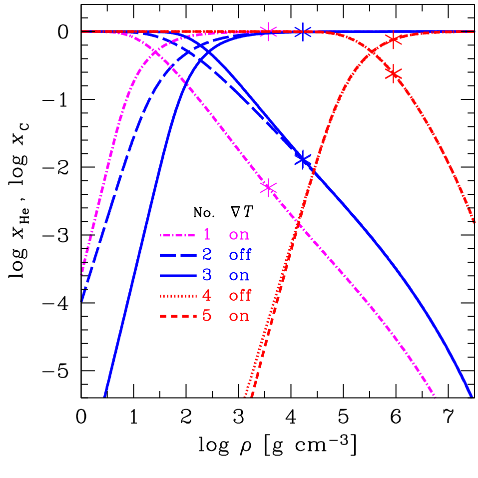
Fig. 1 illustrates the distribution of ions and the temperature profiles $T(\rho)$ in the He – C and C – Fe envelopes with $\rho_{\mathrm{b}}=10^{10}$ g cm^-3. Calculations are performed for two surface temperatures, $T_{\mathrm{s}}=$ 0.8 and 1.5 MK (solid and dashed lines, respectively). The total amount of lighter ions is fixed to $\rho^{*}=10^{6}$ g cm^-3 for the He – C envelope (black lines), and to $10^{8}$ g cm^-3 for the C – Fe one (grey lines). Accordingly, the transition layer from lighter ions to heavier ones for the C – Fe envelope lies deeper. The assumed $\rho^{*}$ in the He – C envelope corresponds to the geometrical depth $z^{*}\approx 3$ m, and the bottom depth of the envelope is $z_{\mathrm{b}}\approx 161$ m; for the C – Fe envelope, we have $z^{*}\approx 28$ m and $z_{\mathrm{b}}\approx 145$ m.

The left-hand panel of Fig. 1 demonstrates the density dependence of the number fraction $x_{1}$ of lighter ions (He for He – C; C for C – Fe). One can observe different profiles $x_{1}(\rho)$ for the He – C and C – Fe envelopes. Characteristic relative width $\delta\rho/\rho^{*}$ of the transition layer in the He – C envelope is typically more than ten times larger than in the C – Fe envelope. This results from much weaker (Coulomb) separation in the He – C mixture. If the separation of ions is gravitational (as in C – Fe or H – He BIMs) a transition from lighter to heavier ions in diffusive equilibrium is rather sharp, but in case of Coulomb separation (He – C) it is broad (similar conclusion has been made by Chang et al. 2010). There appears a tail of He ions at densities much larger than $\rho^{*}$; these ions constitute a noticeable fraction of the total He mass, $\Delta M$. Of course, similar tail exists also in the C – Fe mixture, but it is much less pronounced. When $T_{\mathrm{s}}$ decreases, the envelopes become colder and the transition layers narrower.

The right-hand panel of Fig. 1 shows the temperature $T$ versus density in the same envelopes. Because the He – C envelope consists of lighter ions, it is overall more heat transparent, than the C – Fe envelope, and has a lower $T(\rho)$ for the same $T_{\mathrm{s}}$. For the densities close to $10^{10}$ g cm^-3 the thermal conductivity becomes so high that the temperature $T(\rho)$ tends to saturate reaching the temperature of nearly isothermal matter behind the heat blanketing envelope (Gudmundsson et al. 1983; Potekhin et al. 1997).

Fig. 2 displays the $T_{\mathrm{b}}-T_{\mathrm{s}}$ relations calculated for the He – C and C – Fe envelopes with $\rho_{\mathrm{b}}=10^{10}$ g cm^-3. In case of the He – C envelope, we plot $T_{\mathrm{b}}-T_{\mathrm{s}}$ at $\rho^{*}=10^{6}$ and $10^{8}$ g cm^-3; while for the C – Fe envelope at $\rho^{*}=10^{8}$ and $10^{9}$ g cm^-3. Because the He – C envelope is overall more heat transparent, it has a lower $T_{\mathrm{b}}$ for the same $T_{\mathrm{s}}$. By increasing $\rho^{*}$ we increase the amount of lighter ions in a given envelope, which also increases the heat transparency (at sufficiently high $\rho$) and decreases $T_{\mathrm{b}}$ (at sufficiently high $T_{\mathrm{s}}$ at which the main temperature gradient reaches the range of $\rho\sim\rho^{*}$).

Fig. 3 shows typical $T_{\mathrm{b}}-T_{\mathrm{s}}$ relations for the He – C (left-hand panel) and C – Fe (right-hand panel) envelopes. On each panel we plot $T_{\mathrm{b}}-T_{\mathrm{s}}$ for an envelope containing pure lighter ions (He or C); pure heavier ions (C or Fe); and a mix appropriate to $\rho^{*}=10^{6}$ g cm^-3. Envelopes of pure lighter ions are better heat conductors and have lower $T_{\mathrm{b}}(T_{\mathrm{s}})$. Envelopes of pure heavier ions are better heat insulators and have higher $T_{\mathrm{b}}(T_{\mathrm{s}})$. Envelopes containing BIMs produce intermediate heat insulation. Increasing $\rho^{*}$ varies their insulation from that for heavier ions to that for lighter ones.

Fig. 4 demonstrates the dependence of $T_{\mathrm{b}}$ on the transition density $\rho^{*}$ for the H – He (left-hand panel) and He – C (right-hand panel) envelopes. The surface temperature is fixed to $T_{\mathrm{s}}=1.47$ MK. The solid lines are calculated assuming $\rho_{\mathrm{b}}=10^{8}$ g cm^-3, the short-dashed lines are for $\rho_{\mathrm{b}}=10^{9}$ g cm^-3 and the long-dashed line for the He – C envelope is for $\rho_{\mathrm{b}}=10^{10}$ g cm^-3. We do not present similar line for the H – He envelope because He cannot survive at such high densities (Sect. 5). Any line exhibits a transition from the regime of low $\rho^{*}$, where the amount of lighter ions is small and the envelope behaves as almost fully composed of heavier ions, to the regime of high $\rho^{*}$, where the amount of heavier ions is small and the envelope behaves as if it consists of lighter ions. The ranges of intermediate $\rho^{*}$ in which the binary composition is really significant are seen to be wide.

Notice the anomalous behavior of the H – He BIM. For this BIM, contrary to the He – C and C – Fe BIMs, increasing the amount of lighter (hydrogen) ions leads to the growth of $T_{\mathrm{b}}$. This effect has been overlooked in previous studies (see, e.g., Potekhin et al. 1997) which stated that replacing He with H does not affect $T_{\mathrm{b}}$. The effect is mainly because hydrogen has a different mass to charge ratio than helium and carbon, and also because of low radiative opacities of helium. A C – Fe mixture has the same transition ‘direction’ as He – C mixture since the mass to charge ratio of iron is not very different from that of carbon (unlike hydrogen where the difference is larger).

Fig. 5 shows the impact of the $\bm{\nabla}T$ term in equation (2), or in (14), on the properties of He – C envelopes. The figure shows the helium fraction profile $x_{\mathrm{He}}(\rho)$ calculated in five cases (curves 1 – 5) for the same surface temperature $T_{\mathrm{s}}=1.1$ MK. Cases 1, 3, and 5 are calculated with account of the $\bm{\nabla}T$ term, whereas in cases 2 and 4 this term is neglected (which is equivalent to the approximation made by Chang et al. 2010; Beznogov & Yakovlev 2013). The curves 2 and 3 are computed for the same effective transition density $\rho^{*}\approx 1.7\times 10^{4}$ g cm^-3, whereas model 1 has the same trace amount of carbon with model 2 at the radiative surface, from which we start the integration [$x_{\mathrm{C}}(z=0)=2\times 10^{-6}$]. The latter boundary condition leads to a different accumulated He mass, that is to different transition density $\rho^{*}\approx 3.7\times 10^{3}$ g cm^-3. However, the differences between the curves 1, 2 and 3 are insignificant for the $T_{\mathrm{b}}-T_{\mathrm{s}}$ relation. The calculated $T_{\mathrm{b}}$ values differ by $\lesssim 1$ per cent, because the corresponding $\rho^{*}$ lie outside the ‘sensitivity strip’ (Gudmundsson et al., 1983) which is the $\rho-T$ domain where the conductivity affects the $T_{\mathrm{b}}-T_{\mathrm{s}}$ relation most significantly. At contrast, both models 4 and 5 have $\rho^{*}\approx 9\times 10^{5}$ g cm^-3 inside the sensitivity strip, but in this case the $\bm{\nabla}T$ term is less significant because of stronger degeneracy. As a consequence, the curves 4 and 5 are very close to each other, so that the $\bm{\nabla}T$ term is also unimportant for the $T_{\mathrm{b}}-T_{\mathrm{s}}$ relation (the difference in $T_{\mathrm{b}}$ is again within 1 per cent).

We note that in the cases 1 – 3 the He abundance is quite low, $x_{\mathrm{He}}\lesssim 0.01$, at the transition density $\rho^{*}$. This reflects the fact that in these three cases the layer with high He abundance is mostly nondegenerate, but a considerable fraction of the total He mass is supplied by a diffusive tail in the deeper degenerate layers of the envelope.

Our calculations show that the $\bm{\nabla}T$ term significantly affects the ion fractions if the layer, where the ion Coulomb coupling is moderate (neither weak nor strong), is close to the layer, where a transition from lighter to heavier ions takes place. Such situations may occur at sufficiently high $T_{\mathrm{s}}$ in the outer layers ($\rho\lesssim 10^{7}$ g cm^-3) of the envelopes composed of sufficiently light elements like hydrogen, helium or carbon. Even in these cases the $T_{\mathrm{b}}-T_{\mathrm{s}}$ relations, the pressure and total density profiles are affected much weaker by the $\bm{\nabla}T$ term. Moreover, in the limit of strong Coulomb coupling (described, e.g. in Beznogov & Yakovlev 2013) the $\bm{\nabla}T$ term vanishes completely and non-isothermal calculations coincide exactly with isothermal ones (as long as we do not take into account thermal diffusion).

Finally, Fig. 6 illustrates another important feature of heat blanketing envelopes which is not related directly to their multicomponent structure. Specifically, it concerns the meaning of $\rho_{\mathrm{b}}$. If one integrates the equations of thermal structure for a heat blanketing envelope from the surface to the bottom ($\rho=\rho_{\mathrm{b}}$), one often obtains (e.g. Fig. 2) that the growth of $T(\rho)$ nearly saturates at some $\rho=\rho_{\mathrm{b}}^{*}<\rho_{\mathrm{b}}$. This saturation is evidently associated with the growth of the thermal conductivity within the star. It is especially pronounced in a cold neutron star manifesting the appearance of the inner isothermal region $\rho>\rho_{\mathrm{b}}^{*}$ within the star. In contrast to the density $\rho_{\mathrm{b}}$ which is artificially assumed, $\rho_{\mathrm{b}}^{*}$ can be viewed as a real physical bottom density of the heat blanketing envelope. Fig. 6 shows this density for a ‘canonical’ neutron star, whose envelope consists solely either of iron or carbon. In a hot star ($T_{\mathrm{s}}\sim 3$ MK), the physical heat blanket is thick (close to the assumed heat blanket with $\rho_{\mathrm{b}}\sim 10^{10}$ g cm^-3). However when the star cools, $\rho_{\mathrm{b}}^{*}$ decreases, implying that $T_{\mathrm{b}}$ is actually determined by a much thinner ‘physical’ heat insulating layer. For instance, at $T_{\mathrm{s}}=1$ MK we have $\rho_{\mathrm{b}}^{*}\lesssim 10^{7}$ g cm^-3 so that $T_{\mathrm{b}}$ becomes insensitive to the physics of matter at higher densities (to the composition of such a matter and to whether it is liquid or solid). The colder the star, the thinner the ‘physical’ heat blanket. On the other hand, let us remind that the blanket can become thick, with $\rho_{\mathrm{b}}^{*}>10^{10}$ g cm^-3, for magnetars, as shown by Potekhin et al. (2007). In a multilayer heat blanketing envelope it is also possible to encounter a ‘false physical bottom’, where $T(\rho)$ saturates at certain $\rho_{\mathrm{b}}^{*}$, but resumes its growth at a larger density when it enters a layer with a higher $Z$.

In addition to diffusively equilibrated heat blanketing envelopes considered above, we have also studied the envelopes out of diffusive equilibrium. Since ion diffusion is rather slow (see below) such envelopes can exist for a long time (being, of course, in the overall hydrostatic equilibrium). For illustration, we study them in a quasi-statical approximation, fix the distribution of ions, $x_{j}(\rho)$, disregard the diffusive equilibrium and calculate the structure of the envelopes by integrating equations (16). This is much easier than respect the diffusive equilibrium.

Some illustrative results are shown in Fig. 7. On the left-hand panel we present three models of H – He envelopes, and on the right-hand panel three models of He – C envelopes. The figure shows the profile of the helium number fraction $x_{\mathrm{He}}$ versus $\rho$ for a ‘canonical’ neutron star. The surface temperature is fixed to $T_{\mathrm{s}}=1$ MK for all models. All the three H – He models have the same amount of hydrogen ($\log\rho^{*}=5.06$ [ g cm^-3]) and all the three He – C models the same amount of He ($\log\rho^{*}=7.18$). The helium fraction decreases with $\rho$ on the left-hand panel (because He ions are heavier than H) and increases with $\rho$ on the right-hand panel (because He ions are lighter than C ones). The solid line on each panel corresponds to diffusively equilibrated envelopes (calculated as described in the previous sections). The dashed lines are for the envelopes taken to be out of diffusive equilibrium. The short-dashed lines refer to narrower (than in diffusive equilibrium) transition layers while the long-dashed lines refer to wider layers.

It is remarkable, that for all the three He – C models we obtain almost the same $T_{\mathrm{b}}=4.00\times 10^{7}$ K (which we present for $\rho_{\mathrm{b}}=10^{10}$ g cm^-3, as an example). The same is true for H – He models. For instance, assuming $\rho_{\mathrm{b}}=10^{9}$ g cm^-3 we have $T_{\mathrm{b}}=4.64\times 10^{7}$ K for the equilibrium and narrower transition layers and $T_{\mathrm{b}}=4.54\times 10^{7}$ K for the wider transition layer. Therefore, the resulting $T_{\mathrm{b}}-T_{\mathrm{s}}$ relations seem highly insensitive to the actual state of the envelope, whether it is equilibrated or not. These $T_{\mathrm{b}}-T_{\mathrm{s}}$ relations are mainly determined by the mass $\Delta M$ of lighter ions (or, equivalently, by $\rho^{*}$). Of course, this statement is true for the envelopes where the distribution of ions is not too much wider than the equilibrium one. This is illustrated by a relatively large deviation from the equilibrium for the wider H – He distribution; in this case $T_{\mathrm{b}}$ becomes slightly different from the equilibrium one. However, large deviations from equilibrium are expected to relax at short timescales (days to years, see below).

The insensitivity of $T_{\mathrm{b}}-T_{\mathrm{s}}$ relations to number fraction distributions throughout the envelopes also answers the question on thermal diffusion. Although thermal diffusion can change the ion fractions, this change would not affect the resulting $T_{\mathrm{b}}-T_{\mathrm{s}}$ relation. However, if one is interested in the processes which are sensitive to number fractions (e.g., diffusive nuclear burning) then thermal diffusion can be important. We have made order of magnitude estimates of the impact of thermal diffusion on the diffusion velocity. We have assumed a constant thermal diffusion ratio $k_{T}=0.1$. This is a conservative upper limit obtained in our calculations with the effective potential method described by Beznogov & Yakovlev 2014a; real values are smaller. For H – He mixture ($x_{\mathrm{H}}=x_{\mathrm{He}}=0.5$) the thermal diffusion correction to the diffusion velocity does not exceed 3 per cent, while for He – C mixture ($x_{\mathrm{He}}=x_{\mathrm{C}}=0.5$) it does not exceed 6 per cent. This correction has its largest value near the surface where the temperature gradient is big (see, e.g., the right-hand panel of Fig. 1) and decreases with depth.

Using equation (12) and taking typical depth-scales $\Delta z$ of deviations from diffusive equilibrium in the transition layer, for the conditions in Fig. 7 we can estimate characteristic relative velocities $V$ of two ion species during diffusive equilibration in that layer and typical equilibration times $t_{\mathrm{eq}}\sim\Delta z/V$. For H – He envelopes (left-hand panel) we very roughly obtain $\Delta z\sim$ a few meters, the equilibration velocity $V\sim 10^{-4}-10^{-3}$ cm s^-1, and the equilibration time $t_{\mathrm{eq}}\sim$ one or a few days. For He – C envelopes (right-hand panel) we also have $\Delta z\sim$ a few meters, but the diffusive velocities $V\sim 10^{-7}-10^{-6}$ cm s^-1 are lower, and $t_{\mathrm{eq}}\sim$ a few years. The equilibration in the He – C envelopes goes much slower because of weaker Coulomb separation and deeper transition layer. Our example shows that the He – C envelopes can be out of diffusive equilibrium for a long time.

We have considered two-component heat blanketing envelopes of neutron stars. These envelopes can be either in diffusive equilibrium or out of it. Our main goal has been to relate the effective surface temperature of the star, $T_{\mathrm{s}}$, to the temperature $T_{\mathrm{b}}$ at the bottom of the envelope ($\rho=\rho_{\mathrm{b}}\sim 10^{8}-10^{10}$ g cm^-3) and to investigate the sensitivity of this relation to the distribution of ion species within the envelope.

We have derived general expressions for the diffusive fluxes in multicomponent non-isothermal gaseous or liquid Coulomb systems of ions with arbitrary Coulomb coupling taking into account temperature gradient. In the limit of weakly coupled plasma these expressions reproduce the classical expressions for diffusion in ideal gas mixtures. Our new expressions are valid not only for Coulomb systems, but also for any gaseous or liquid system (diffusion is also available in solids, e.g. Hughto et al. 2011, but it is greatly suppressed there compared to gases and liquids).

For applications, we have calculated the $T_{\mathrm{b}}-T_{\mathrm{s}}$ relations for two component envelopes (containing H – He, He – C, or C – Fe mixtures). These envelopes are naturally stratified into three layers. The outer layer consists predominantly of lighter ions; the inner layer near the envelope bottom contains mainly heavier ions; and there is a transition layer of essentially binary mixture in between. The stratification in the H – He and C – Fe envelopes, where two ion species have different ‘molecular weights’, is mainly gravitational; while in the He – C envelopes it is much weaker (Coulombic). Accordingly, the transition layers in the He – C envelopes are much wider than in other envelopes. The $T_{\mathrm{b}}-T_{\mathrm{s}}$ relations have been determined for diffusively equilibrated envelopes with different mass $\Delta M$ of lighter ions (or, equivalently, with different characteristic densities $\rho^{*}$ which specify the position of the transition layer). The results are approximated by analytic expressions in Appendix A, which can be used for simulating thermal evolution of isolated and accreting neutron stars and related phenomena (e.g., Chang & Bildsten 2003; Chang & Bildsten 2004; Yakovlev & Pethick 2004; Chang et al. 2010; Potekhin et al. 2015).

The most striking result of our analysis is that the $T_{\mathrm{b}}-T_{\mathrm{s}}$ relations are fairly independent of the structure of the transition layer (of its width, distribution of ions, and of whether it is diffusively equilibrated or not). These relations depend only on $\Delta M$ (or on $\rho^{*}$). This allows us to expect that the fit expressions presented in Appendix A can be used not only for diffusively equilibrated envelopes but also for a much wider class of envelope models. In particular, this remarkable property justifies previous studies (Potekhin et al., 1997; Yakovlev et al., 2011) of heat blanketing envelopes as a sequence of layers composed of single ion species (e.g., H, He, C, Fe); slow diffusion of ions does not introduce noticeable changes in $T_{\mathrm{b}}-T_{\mathrm{s}}$ relations. However, nuclear transformations, which can noticeably change $\Delta M$, can affect these relations indirectly (Chang & Bildsten, 2004; Chang et al., 2010).

Thus, we have confirmed the previous $T_{\mathrm{b}}-T_{\mathrm{s}}$ relations and extended their studies. First of all, we have considered H – He and He – C envelopes, and approximated the appropriate $T_{\mathrm{b}}-T_{\mathrm{s}}$ relations by analytic expressions for different $\rho^{*}$ and $\rho_{\mathrm{b}}$ in Appendix A. We have also reconsidered C–Fe envelopes, found good agreement with previous results (Yakovlev et al., 2011), and fitted the $T_{\mathrm{b}}-T_{\mathrm{s}}$ relations (Appendix A).

It is evident that our two-component envelopes are idealized; real envelopes may contain much more ion components. However, ion stratification seems to be rather strong to prevent the appearance of layers of essentially multicomponent mixtures if the heat blanketing envelopes contain many ion species. It is likely that real envelopes have onion-like structure. Let us stress once more a great difference of gravitational and Coulomb stratifications. The latter one is much slower so that the ions with the same charge-to-mass ratio (like He and C) are mixed much easier than other ions, have much thicker transition layers, and can be out of diffusive equilibrium for a longer time. They can form much more extended ‘tails’ outside the transition layer which can affect nuclear burning, thermal conduction and other processes important for thermal structure and evolution of neutron stars. Similar stratification features may be important in white dwarfs.

The expressions for the diffusive fluxes combined with the diffusion coefficients (see, e.g., Beznogov & Yakovlev 2014a) allow one not only to calculate the diffusively equilibrated configurations of heat blanketing envelopes of neutron stars, but also the equilibration of these configurations with time.

The work of MB was partly supported by the Dynasty Foundation, and the work of AP by the Russian Foundation for Basic Research (grant 14-02-00868-a).

References

- Akmal et al. (1998) Akmal A., Pandharipande V. R., Ravenhall D. G., 1998, Phys. Rev. C, 58, 1804
- Beznogov & Yakovlev (2013) Beznogov M. V., Yakovlev D. G., 2013, Phys. Rev. Lett., 111, 161101
- Beznogov & Yakovlev (2014a) Beznogov M. V., Yakovlev D. G., 2014a, Phys. Rev. E, 90, 033102
- Beznogov & Yakovlev (2014b) Beznogov M. V., Yakovlev D. G., 2014b, J. Phys.: Conf. Ser., 572, 012001
- Chang & Bildsten (2003) Chang P., Bildsten L., 2003, ApJ, 585, 464
- Chang & Bildsten (2004) Chang P., Bildsten L., 2004, ApJ, 605, 830
- Chang et al. (2010) Chang P., Bildsten L., Arras P., 2010, ApJ, 723, 719
- De Blasio (2000) De Blasio F. V., 2000, A&A, 353, 1129
- Goriely et al. (2010) Goriely S., Chamel N., Pearson J. M., 2010, Phys. Rev. C, 82, 035804
- Gudmundsson et al. (1983) Gudmundsson E. H., Pethick C. J., Epstein R. I., 1983, ApJ, 272, 286
- Haensel et al. (2007) Haensel P., Potekhin A. Y., Yakovlev D. G., 2007, Neutron Stars. 1. Equation of State and Structure. Astrophysics and Space Science Library Vol. 326, Springer, New York
- Hameury et al. (1983) Hameury J. M., Heyvaerts J., Bonazzola S., 1983, A&A, 121, 259
- Hirschfelder et al. (1954) Hirschfelder J. O., Curtiss C. F., Bird R. B., 1954, Molecular Theory of Gases and Liquids. Wiley, New York
- Hughto et al. (2011) Hughto J., Schneider A. S., Horowitz C. J., Berry D. K., 2011, Phys. Rev. E, 84, 016401
- Kaminker et al. (2009) Kaminker A. D., Potekhin A. Y., Yakovlev D. G., Chabrier G., 2009, MNRAS, 395, 2257
- Landau & Lifshitz (1993) Landau L. D., Lifshitz E. M., 1993, Statistical Physics, Part 1. Pergamon, Oxford
- Lattimer (2014) Lattimer J. M., 2014, General Relativity and Gravitation, 46, 1713
- Lifshitz & Pitaevskiĭ (1981) Lifshitz E. M., Pitaevskiĭ L. P., 1981, Physical Kinetics. Pergamon, Oxford
- Mendoza et al. (2007) Mendoza C., et al., 2007, MNRAS, 378, 1031
- Ofengeim et al. (2015) Ofengeim D. D., Kaminker A. D., Klochkov D., Suleimanov V., Yakovlev D. G., 2015, MNRAS, 454, 2668
- Paquette et al. (1986) Paquette C., Pelletier C., Fontaine G., Michaud G., 1986, ApJS, 61, 177
- Paxton et al. (2015) Paxton B., et al., 2015, ApJS, 220, 15
- Potekhin & Chabrier (2010) Potekhin A. Y., Chabrier G., 2010, Contrib. Plasma Phys., 50, 82
- Potekhin et al. (1997) Potekhin A. Y., Chabrier G., Yakovlev D. G., 1997, A&A, 323, 415
- Potekhin et al. (2003) Potekhin A. Y., Yakovlev D. G., Chabrier G., Gnedin O. Y., 2003, ApJ, 594, 404
- Potekhin et al. (2007) Potekhin A. Y., Chabrier G., Yakovlev D. G., 2007, Ap&SS, 308, 353
- Potekhin et al. (2013) Potekhin A. Y., Fantina A. F., Chamel N., Pearson J. M., Goriely S., 2013, A&A, 560, A48
- Potekhin et al. (2015) Potekhin A. Y., Pons J. A., Page D., 2015, Space Sci. Rev., 191, 239
- Rogers et al. (1996) Rogers F. J., Swenson F. J., Iglesias C. A., 1996, ApJ, 456, 902
- Viganò et al. (2013) Viganò D., Rea N., Pons J. A., Perna R., Aguilera D. N., Miralles J. A., 2013, MNRAS, 434, 123
- Weisskopf et al. (2011) Weisskopf M. C., Tennant A. F., Yakovlev D. G., Harding A., Zavlin V. E., O’Dell S. L., Elsner R. F., Becker W., 2011, ApJ, 743, 139
- Yakovlev & Pethick (2004) Yakovlev D. G., Pethick C. J., 2004, ARA&A, 42, 169
- Yakovlev et al. (2011) Yakovlev D. G., Ho W. C. G., Shternin P. S., Heinke C. O., Potekhin A. Y., 2011, MNRAS, 411, 1977
Appendix A Data fitting