Local pinning of networks of multi-agent systems with transmission and pinning delays

First, we take $\tau_{p}=0$ and prove stability for all $\tau_{r}\geq 0$. Assume for contradiction that there exists some characteristic root $\lambda^{*}$ of (5) such that $\mathrm{Re}(\lambda^{*})\geq 0$. Applying the Gershgorin disc theorem to (5), we have

$$|\lambda^{*}+L_{ii}+cd_{i}|\leq\sum_{j\neq i}|L_{ij}||\exp(-\lambda^{*}\tau_{r})|\leq\sum_{j\neq i}|L_{ij}|=L_{ii}$$

(8)

for some $i$, which implies

$$[\mathrm{Re}(\lambda^{*})+L_{ii}+cd_{i}]^{2}+[{\mathrm{Im}}(\lambda^{*})]^{2}\leq L_{ii}^{2}.$$

Since $L_{ii},c,d_{i}\geq 0$, it must be the case that $\mathrm{Re}(\lambda^{*})=\mathrm{Im}(\lambda^{*})=0$; i.e., $\lambda^{*}=0$. Then $\exp(-\tau_{r}\lambda^{*})=1$, and since $\tau_{p}=0$, (5) gives $\det(\lambda^{*}I_{n}+L+cD)=0$. This, however, contradicts Corollary 1. Therefore, when $\tau_{p}=0$, all characteristic roots of (5) have negative real parts.

We now let $\tau_{p}\geq 0$. Suppose (5) has a purely imaginary root $\lambda=\mathbf{j}\omega$, $\omega\in\mathbb{R}$. By (8), we have, for some index $q$,

	$\displaystyle|\mathbf{j}\omega+L_{qq}+cd_{q}\exp(-\mathbf{j}\omega\tau_{p})|\leq\sum_{j\neq q}|L_{qj}||\exp(-\mathbf{j}\omega\tau_{r})$
	$\displaystyle=\sum_{j\neq q}|L_{qj}|=L_{qq}$

implying

$$\sqrt{[L_{qq}+cd_{q}\cos(\omega\tau_{p})]^{2}+[\omega-cd_{q}\sin(\omega\tau_{p})]^{2}}\leq L_{qq}.$$

Thus,

$$(cd_{q})^{2}+\omega^{2}+2cd_{q}\left(L_{qq}\cos(\omega\tau_{p})-\omega\sin(\omega\tau_{p})\right)\leq 0.$$

(9)

We claim that $q$ must be a pinned node. For if $d_{q}=0$, then $\omega$ must be zero, which implies that zero is a characteristic root of (5), contradicting Corollary 1. Therefore $d_{q}=1$. In the notation of (6), the inequality (9) can then be written as $F(w,c,L_{qq},\tau_{p})\leq 0$. By (7), however, we have that $F(w,c,L_{qq},\tau_{p})>0$ for all $p\in\mathcal{D}$, $\omega\in{\mathbb{R}}$ and $\tau_{p}<\tau_{p}^{*}$. We conclude that (5) does not have purely imaginary roots for $\tau_{p}<\tau_{p}^{*}$. Thus, by [27, Theorem 2.1], all characteristic roots of (5) have strictly negative real parts for $\tau_{p}<\tau_{p}^{*}$. ∎

As in the first part of the proof of Proposition 2, the equation $\det[\lambda I_{n}+K-A\exp(-\lambda\tau_{r})]=0$ has no solutions with $\mathrm{Re}(\lambda)\geq 0$. Hence, if all solutions $\lambda$ of (11) have negative real parts, then all roots of (5) have negative real parts. ∎

We consider two specific cases to obtain more information about the solutions of (11). First, we consider the absence of transmission delays, i.e., $\tau_{r}=0$. Suppose for simplicity that $L$ is diagonalizable and has only real eigenvalues: $L=Q^{-1}JQ$ for some nonsingular $Q$ and a real diagonal matrix $J=\diag\{\theta_{1},\dots,\theta_{n}\}$ of eigenvalues of $L$. The column vectors of $Q^{-1}$ (resp, the row vectors of $Q$) are the right (resp., left) eigenvectors of $L$. Then, (11) can be written as

$$1+c\zeta^{\top}(\lambda I_{n}+J)^{-1}\xi\exp(-\lambda\tau_{p})=0,$$

(12)

where $\zeta^{\top}=u_{q}^{\top}Q$ is the $q$th left eigenvector and $\xi=Q^{-1}u_{q}$ is the $q$th right eigenvector of $L$. We expand (12) as

$$1+c\sum_{i=1}^{n}\frac{\xi_{i}\zeta_{i}\exp(-\lambda\tau_{p})}{\lambda+\theta_{i}}=0$$

(13)

in terms of the components $\xi_{i},\zeta_{i}$ of $\xi$ and $\zeta$, respectively. Consider the smallest value of $\tau_{p}$ for which there exists a purely imaginary solution, $\lambda=\mathbf{j}\omega$. Then, the real and imaginary parts of (13) give

$$\begin{cases}1+a(\omega)\cos(\omega\tau_{p})-b(\omega)\sin(\omega\tau_{p})&=0\\ b(\omega)\cos(\omega\tau_{p})+a(\omega)\sin(\omega\tau_{p})&=0\end{cases}$$

where

$$a(\omega)=c\sum_{i=1}^{n}\frac{\xi_{i}\zeta_{i}\theta_{i}}{\omega^{2}+\theta_{i}^{2}},\quad b(\omega)=c\sum_{i}\frac{\xi_{i}\zeta_{i}\omega}{\omega^{2}+\theta_{i}^{2}}.$$

(14)

Rearranging gives $\cos(\omega\tau_{p})=-a(\omega)/(a^{2}(\omega)+b^{2}(\omega))$ and $\sin(\omega\tau_{p})=b(\omega)/(a^{2}(\omega)+b^{2}(\omega))$. This implies $a(\omega)^{2}+b^{2}(\omega)=1$ and

$$\cos(\omega\tau_{p})=-a(\omega),\quad\sin(\omega\tau_{p})=b(\omega).$$

(15)

We then have the following result.

Since the graph is strongly connected, $L$ has a simple zero eigenvalue. When $c=0$, the dominant root of (5) is $\sigma_{1}=\lambda_{1}(0)$. Since the roots of (5) depend analytically on $c$, they are given by $\lambda_{1}(c)$ for all sufficiently small $c$. Substituting (22) into $\lambda_{1}(c)$ and noting that ${\psi^{1}}^{\top}(-K+A)\phi^{1}=0$ completes the proof. ∎

In order to understand the meaning of (23), consider the special case of an undirected graph with binary adjacency matrix $A$. Then, with $\phi^{1}=[1,\dots,1]^{\top}$ and $\psi^{1}=[1,\dots,1]^{\top}/n$, we have ${\psi^{1}}^{\top}K\phi^{1}=\sum_{i=1}^{n}L_{ii}/n$, which equals the average degree of the graph. In addition, ${\psi^{1}}^{\top}D\phi^{1}=\sum_{i=1}^{n}\delta_{\mathcal{D}}(i)/n$, which is the fraction of pinned agents. Then, (23) yields the approximation

$$\lambda_{1}(c)\approx-\frac{\textrm{Pinning~Fraction}}{1+\tau_{r}\times\textrm{Mean~Degree}}c$$

(24)

for small $c$, which uses only the pinning fraction and the mean degree of the graph. Since the real part of the dominant characteristic value measures the exponential convergence of the system, Proposition 6 implies that, for sufficiently small $c$, the convergence rate is improved if the number of pinned nodes is increased, the transmission delay is reduced, or the mean degree is decreased. If the graph is directed, a similar statement can be obtained by taking the components of $\psi^{1}$ as weights: $\psi^{1}D\phi^{1}=\sum_{j=1}^{n}\psi^{1}_{j}\delta_{\mathcal{D}}(j)$.

To illustrate this result, we employ a numerical method to calculate the real part of $\lambda_{1}(c)$, namely, by simulating the system (4) and expressing its exponential convergence rate in terms of its largest Lyapunov exponent. In detail, letting $\tau_{m}=\max\{\tau_{r},\tau_{p}\}$, we partition time into disjoint intervals of length $\tau_{m}$, $t_{k}=k\tau_{m}$, and define $\eta_{k}(\theta)=y(t_{k}+\theta)$ for $\theta\in[0,\tau_{m}]$. Then, the largest Lyapunov exponent, which equals to the largest real part of solutions of (5), is numerically calculated via [31]

$$\mathrm{Re}(\lambda_{1,\mathrm{sim}})=\lim_{N\to\infty}\frac{1}{N\tau_{m}}\log\|\eta_{N}\|=\lim_{N\to\infty}\frac{1}{N\tau_{m}}\sum_{k=1}^{N}\log\frac{\|\eta_{k}\|}{\|\eta_{k-1}\|},$$

(25)

where $\|\cdot\|$ stands for the function norm. The latter is numerically calculated by approximating $\eta_{k}(\cdot)$ with a finite-dimensional vector $\varphi_{k}$ obtained by evaluating $\eta_{k}$ at a finite number of equally spaced points and using the vector norm $\|\varphi_{k}\|$. The estimate (25) can then be compared with the analytical estimate for $\mathrm{Re}(\lambda_{1})$ obtained from (23):

$$\mathrm{Re}(\lambda_{1,\mathrm{est}})=-\frac{{\psi^{1}}^{\top}D\phi^{1}}{1+\tau_{r}({\psi^{1}}^{\top}K\phi^{1})}c.$$

(26)

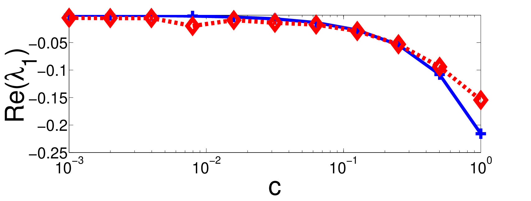
For simulations, we generate an undirected E-R random graph of $n=100$ nodes with linking probability $p=0.03$ and randomly select a given fraction $f$ of them as the pinned nodes. The pinning delay is taken as $\tau_{p}=0.1$. Figure 2 shows that the simulated value of $\mathrm{Re}(\lambda_{1})$ decreases almost linearly with respect to $c$ and $f$, and increases with respect to $\tau_{r}$ and the mean degree. The simulation results are in a good agreement with the theoretical results. The error between $\mathrm{Re}(\lambda_{1,\mathrm{est}})$ and $\mathrm{Re}(\lambda_{1,\mathrm{sim}})$ depends on the values of $\lambda_{1}^{1}$ and $c$. It can be seen that the error will increase as $c$ or $\lambda_{1}^{1}$ (or equivalently, $f$) increases, or else as the mean degree or $\tau_{r}$ decreases.

Next, we consider the case of large $c$. Letting $\epsilon=1/c$ and $\mu=\lambda/c$, (5) is rewritten as

$$\det\left[\mu I_{n}+\epsilon K-\epsilon A\exp(-\mu\tau_{r}/\epsilon)+D\exp(-\mu\tau_{p}/\epsilon)\right]=0.$$

(27)

By the foregoing results, one can see that when $\epsilon$ is sufficiently small, equivalently, $c$ is sufficiently large, the largest admissible pinning delay for (4) approaches zero. It is therefore natural to assume that $\tau_{p}$ depends on $c$ in such a way that $\tau_{p}c$ is bounded as $c$ grows large. Thus, we assume that $\tau_{pc}:=\tau_{p}c$ remains bounded as $c\to\infty$.

When $\epsilon=0$, (27) becomes approximately $\dot{x}=-Dx(t-\tau_{p\infty})$, where $\tau_{p\infty}$ can be any value between $\overline{\lim}_{c\to\infty}\tau_{pc}$ and $\underline{\lim}_{c\to\infty}\tau_{pc}$. In terms of components, $\dot{x}_{i}=-x_{i}(t-\tau_{p\infty})$ if $i\in\mathcal{D}$, and $0$ otherwise. The characteristic equation (27) with $\epsilon=0$ can be written as

$$(\mu+\exp(-\mu\tau_{p\infty}))^{m}\mu^{n-m}=0$$

(28)

where $m=|\mathcal{D}|$. It is known that $\mathrm{Re}(\mu)<0$ for all roots of the function $\mu\mapsto\mu+\exp(-\mu\tau_{p\infty})$ if and only if $\tau_{p\infty}<\frac{\pi}{2}$. Therefore, we impose the condition: $\tau_{p}\,c<\frac{\pi}{2}$.

Thus, the largest real part of the solutions of (28) is zero, and is obtained for the solution $\mu=0$. The corresponding eigenspace has dimension $n-m$ and has the form

$$ES=\{u=[u_{1},\dots,u_{n}]^{\top}\in\mathbb{R}^{n}:~u_{i}=0,~\forall~i\in\mathcal{D}\}.$$

Without loss of generality, we assume $\mathcal{D}=\{1,\dots,m\}$. Thus, we consider perturbation in terms of $\epsilon$ near zero eigenvalues $\mu_{i}$ and its corresponding right and left vectors, $\xi^{i},{\zeta^{i}}^{\top}\in ES$ such that $(\zeta^{i})^{\top}\xi^{i}=1$ and $(\zeta^{j})^{\top}\xi^{i}=0$ if $i\neq j$, $i,j=m+1,\dots,n$. Let $\mu_{i}(\epsilon)$ stand for the perturbed solution of (27), $\tilde{\xi}^{i}(\epsilon)$ and $\tilde{\zeta}^{i}(\epsilon)$ be the corresponding right and left eigenvectors, respectively. By a perturbation expansion,

	$\displaystyle\mu_{i}(\epsilon)$	$\displaystyle=$	$\displaystyle\mu^{1}_{i}\epsilon+o(\epsilon),~\tilde{\xi}^{i}(\epsilon)=\xi^{i}+\xi^{i,1}\epsilon+o(\epsilon)$
	$\displaystyle\tilde{\zeta}^{i}(\epsilon)$	$\displaystyle=$	$\displaystyle\zeta^{i}+\zeta^{i,1}\epsilon+o(\epsilon)$		(29)

as $\epsilon\to 0$. Thus, from (27),

	$\displaystyle\left[-\epsilon K+\epsilon A\exp\left(-\mu_{i}(\epsilon)\frac{\tau_{r}}{\epsilon}\right)-D\exp(-\mu_{i}(\epsilon)\tau_{Pc})\right]\tilde{\xi}^{i}(\epsilon)$
	$\displaystyle=\mu_{i}(\epsilon)\tilde{\xi}^{i}(\epsilon).$

Since $\exp(-\mu_{i}(\epsilon)\tau)=1-\epsilon\mu_{i}^{1}\tau+o(\epsilon)$, by comparing the coefficients of order $1$, we have

$\displaystyle[-K+A\exp(-\mu^{1}_{i}\tau_{r})]\xi^{i}-D\xi^{i,1}=\mu^{1}_{i}\xi^{i}.$

(30)

We write

$$K=\left[\begin{array}[]{ll}K_{1}&0\\ 0&K_{2}\end{array}\right],\;A=\left[\begin{array}[]{ll}A_{11}&A_{12}\\ A_{21}&A_{22}\end{array}\right],\;D=\left[\begin{array}[]{ll}I_{m}&0\\ 0&0\end{array}\right],$$

and $\xi^{i}=[{\xi^{i}_{1}}^{\top}$, ${\xi^{i}_{2}}^{\top}]^{\top}$, $\xi^{i,1}=[{\xi^{i,1}_{1}}^{\top},{\xi^{i,1}_{2}}^{\top}]^{\top}$, with $K_{1}$, $A_{11}$, $\xi^{i}_{1}=0$ and $\xi^{i,1}_{1}$ corresponding to the pinned subset $\mathcal{D}$ of dimension $m$. Then (30) becomes

$$\begin{cases}[-K_{2}+A_{22}\exp(-\mu^{1}_{i}\tau_{r})]\xi^{i}_{2}&=\mu^{1}_{i}\xi^{i}_{2}\\ \exp(-\mu^{1}_{i}\tau_{r})A_{12}\xi^{i}_{2}-\xi^{i,1}_{1}&=0.\end{cases}$$

(31)

We have the following result.

References

- [1] M. H. DeGroot, Reaching a consensus, J. Amer. Statist. Assoc., 69 (1974), 118–121.
- [2] C. Reynolds, Flocks, herds, and schools: A distributed behavioral model, Comput. Graph., 21:4 (1987), 25–34.
- [3] T. Vicsek, A. Czirök, E. Ben-Jacob, I. Cohen and O. Shochet, Novel type of phase transition in a system of self-driven particles, Phys. Rev. Lett., 75 (1995), 1226–1229.
- [4] A. Jadbabaie, J. Lin, and A. S. Morse, Coordination of groups of mobile autonomous agents using nearest neighbor rules, IEEE Trans Automat. Control, 48 (2003), 988–1001.
- [5] J. A. Fax and R. M. Murray, Information flow and cooperative control of vehicle formations, IEEE Trans. Autom. Control, 49 (2004), 1465–1476.
- [6] X. F. Wang, G. Chen, Pinning control of scale-free dynamical network, Physica A, 310(2002), 521–531.
- [7] X. Li, X. F. Wang, G. Chen, Pinning a complex dynamical network to its equilibrium, IEEE Trans. Circuits Syst. I, 51:10 (2004), 2074–2087.
- [8] T. P. Chen, X. W. Liu, W. L. Lu. Pinning complex networks by a single controller. IEEE Trans. Circuits Syst. I, 54:6 (2007), 1317–1326.
- [9] W. L. Lu, X. Li, Z. H. Rong. Global stabilization of complex networks with digraph topologies via a local pinning algorithm. Automatica, 46 (2010), 116–121.
- [10] Q. Song, F. Liu, J. Cao, W. Yu, M-Matrix Strategies for Pinning-Controlled Leader-Following Consensus in Multiagent Systems With Nonlinear Dynamics, IEEE Trans. Cybern., 43:6 (2013), 1688–1697.
- [11] Q. Song, F. Liu, J. Cao, W. Yu, Pinning-Controllability Analysis of Complex Networks: An M-Matrix Approach, IEEE Trans. Circuits Syst.-I, 59:11(2012) 2692–270.
- [12] Q. Song, J. Cao, On Pinning Synchronization Of Directed And Undirected Complex Dynamical Networks, IEEE Trans. Circuits Syst.-I, 57:3(2010), 672–680.
- [13] R. Olfati-Saber and R. M. Murray, Consensus problems in networks of agents with switching topology and time-delays, IEEE Trans. Autom. Control, 49 (2004), 1520–1533.
- [14] F. M. Atay, Consensus in networks under transmission delays and the normalized Laplacian. Phil. Trans. Roy. Soc. A, 371 (2013), 20120460.
- [15] F. M. Atay, On the duality between consensus problems and Markov processes, with application to delay systems. Markov Processes and Related Fields (in press).
- [16] P.-A. Bliman and G. Ferrari-Trecate, Average consensus problems in networks of agents with delayed communications, Automatica, 44 (2008), 1985–1995.
- [17] L. Moreau, Stability of multiagent systems with time-dependent communication links, IEEE Trans. Autom. Control, 50 (2005), 169–182.
- [18] F. Xiao and L. Wang, Asynchronous consensus in continuous-time multi-agent systems with switching topology and time-varying delays, IEEE Trans. Autom. Control, 53 (2008), 1804–1816.
- [19] W. L. Lu, F. M. Atay, J. Jost, Consensus and synchronization in discrete-time networks of multi-agents with stochastically switching topologies and time delays, Networks and Heterogeneous Media, 6:2(2011), 329–349.
- [20] L. Xiang, Z. Chen, Z. Liu et al. Pinning control of complex dynamical networks with heterogeneous delays, Computers & Mathematics with Applications, 56:5 (2008), 1423–1433.
- [21] M. Ulrich, A. Papachristodoulou, F. Allgöwer, Generalized Nyquist consensus condition for linear multi-agent systems with heterogeneous delays, Proc. IFAC Workshop on Estimation and Control of Networked Systems, 24–29, 2009.
- [22] P. Andrey, H. Werner, Robust stability of a multi-agent system under arbitrary and time-varying communication topologies and communication delays, IEEE Trans. Autom. Control, 57:9(2012), 2343–2347.
- [23] Z.X. Liu, Z.Q. Chen, Z.Z. Yuan, Pinning control of weighted general complex dynamical networks with time delay, Physica A, 375:1 (2007), 345–354.
- [24] J. Zhao, J.-A. Lu, and Q. Zhang, Pinning a complex delayed dynamical network to a homogeneous trajectory, IEEE Trans. Circuits Syst.-II, 56:6 (2009), 514–518.
- [25] W. Gu, Lag synchronization of complex networks via pinning control, Nonlinear Analysis: Real World Applications, 12:5 (2011), 2579–2585.
- [26] Q. Song, J. Cao, F. Liu, W. Yu, Pinning-controlled synchronization of hybrid-coupled complex dynamical networks with mixed time-delays, Inter. J. Robust Nonlin. Control, 22(2012), 690–706
- [27] S. Ruan, J. Wei. On the zeros of transcendental functions with applications to stability of delay differential equations with two delays. Dynam. Contin. Discrete Impuls. Systems, Ser. A 10 (2003), 863–874.
- [28] R. M. Corless, G. H. Gonnet, D. E. G. Hare, D. J. Jeffrey, D. E. Knuth. On the Lambert W function. Adv. Comput. Math. 5 (1996), 329–359.
- [29] L. N. Trefethen. Numerical Linear Algebra. SIAM (Philadelphia, PA), p. 287 1997.
- [30] R.-C. Li. Matrix Perturbation Theory. In Hogben, Leslie. Handbook of Linear Algebra (2nd ed.), 2014.
- [31] J. D. Farmer, Chaotic attractors of an infinite-dimensional dynamical system, Physica D, 4:3 (1982), 366–393.