跳到论文正文
W Papers独立论文阅读器 arXiv:1604.00431 论文正文 计算阅读时间 · 0%
引用这篇论文根据当前论文元数据生成,正式投稿前建议核对。


License: arXiv.org perpetual non-exclusive license
arXiv:1604.00431v3 [math.DS] 30 Sep 2016

Homoclinic Bifurcations that Give Rise to Heterodimensional Cycles near A Saddle-Focus Equilibrium

DONGCHEN LI
Department of Mathematics, Imperial College London
180 Queen’s Gate, London SW7 2AZ, United Kingdom

†† Date: May 6, 2016.
This work was supported by grant RSF 14-41-00044 at Lobachevsky University of Nizhny Novgorod. The author also acknowledges support by the Royal Society grant IE141468 and EU Marie-Curie IRSES Brazilian-European partnership in Dynamical Systems (FP7-PEOPLE-2012-IRSES 318999 BREUDS).

Abstract. We show that heterodimensional cycles can be born at the bifurcations of a pair of homoclinic loops to a saddle-focus equilibrium for flows in dimension 4 and higher. In addition to the classical heterodimensional connection between two periodic orbits, we found, in intermediate steps, two new types of heterodimensional connections: one is a heteroclinic between a homoclinic loop and a periodic orbit with a 2-dimensional unstable manifold, and the other connects a saddle-focus equilibrium to a periodic orbit with a 3-dimensional unstable manifold.

Keywords. heterodimensional cycle, homoclinic bifurcation, heteroclinic orbit, saddle-focus, chaotic dynamics.

AMS subject classification. 37G20, 37G25.

1 Introduction

For multidimensional systems, i.e. 4-dimensional flows and 3-dimensional maps, the existence of heterodimensional cycles is a main mechanism that leads to non-hyperbolicity (see [4]). A heterodimensional cycle is created by two heteroclinic connections between two saddle periodic orbits with different indices (dimensions of the unstable invariant manifolds). These cycles can be persistent: even when removed by a small perturbation of the system they can re-emerge after an additional arbitrarily small perturbation (see [9, 10, 11, 3]). Thus, they give a mechanism for a persistent coexistence of saddles with different dimension of the unstable manifold within the same chaotic attractor. These attractors should exhibit properties different from those predicted by hyperbolic theory, e.g. the shadowing property could be violated (see [8]). Therefore, the study of heterodimensional cycles is important for a further advancement of the theory of multidimensional chaos.

In this paper, we consider multidimensional flows with two Shilnikov loops (i.e. homoclinic loops to a saddle-focus equilibrium) and show under which conditions their bifurcations can create heterodimensional cycles. As intermediate steps, we find two new types of heterodimentional connections. One type of the connection is between a homoclinic loop and a periodic orbit of index 2, and the other one is between a saddle-focus equilibrium and a periodic orbit of index 3; studying these bifurcations could be of independent interest.

We consider a CrC^{r}-flow XX in ℝn\mathbb{R}^{n} (where r⩾3,n⩾4r\geqslant 3,n\geqslant 4), which has an equilibrium OO of saddle-focus type. The eigenvalues of the linearized matrix of XX at OO are

γ,−λ+ω​i,−λ−ω​i,αj\gamma,-\lambda+\omega i,-\lambda-\omega i,\alpha_{j}

where Re(αj)<−λ<0<γ(\alpha_{j})<-\lambda<0<\gamma (j=1,2​…​n−3j=1,2\ldots n-3), ω≠0\omega\neq 0, and we assume

ρ=λγ<12.\rho=\dfrac{\lambda}{\gamma}<\dfrac{1}{2}. (1)

From now on we let γ=1\gamma=1 (this can always be achieved by time scaling). It follows from the result in Appendix A of [22] that the system near OO can be brought to the form

y˙=y,x1˙=−ρ​x1−ω​x2+f11​(x,y,z)​x+f12​(x,y,z)​z,x2˙=ω​x1−ρ​x2+f21​(x,y,z)​x+f22​(x,y,z)​z,z˙=B​z+f31​(x,y,z)​x+f32​(x,y,z)​z,\begin{array}[]{rcl}\dot{y}&=&y,\\[5.0pt] \dot{x_{1}}&=&-\rho x_{1}-\omega x_{2}+f_{11}(x,y,z)x+f_{12}(x,y,z)z,\\[5.0pt] \dot{x_{2}}&=&\omega x_{1}-\rho x_{2}+f_{21}(x,y,z)x+f_{22}(x,y,z)z,\\[5.0pt] \dot{z}&=&Bz+f_{31}(x,y,z)x+f_{32}(x,y,z)z,\end{array} (2)

by some Cr−1C^{r-1}-transformations of coordinates and time, where x=(x1,x2)x=(x_{1},x_{2}), and the eigenvalues of matrix BB are α1​…​αn−3\alpha_{1}\ldots\alpha_{n-3}. Functions fi​jf_{ij} are Cr−1C^{r-1}-smooth and satisfy

fi​j(0,0,0)=0,f1​j(x,0,z)≡0,f2​j(x,0,z)≡0,fi​1(0,y,0)≡0(i=1,2,3 and j=1,2).f_{ij}(0,0,0)=0,\quad f_{1j}(x,0,z)\equiv 0,\quad f_{2j}(x,0,z)\equiv 0,\quad f_{i1}(0,y,0)\equiv 0\quad(i=1,2,3\mbox{ and }j=1,2). (3)

In such coordinate system, the coordinates of OO are (0,0,0)(0,0,0) and the local invariant manifolds are straightened, i.e., Wl​o​cu(O)={x=0,z=0},Wl​o​cs(O)={y=0}W^{u}_{loc}(O)=\{x=0,z=0\},W^{s}_{loc}(O)=\{y=0\} and Wl​o​cs​s​(O)={x=0,y=0}W^{ss}_{loc}(O)=\{x=0,y=0\}.

The one-dimensional unstable manifold of OO consists of two separatrices; the upper one, Γ+\Gamma^{+} corresponds, locally, to y>0y>0 and the lower separatrix Γ−\Gamma^{-} corresponds to y<0y<0. Let the separatrices Γ+\Gamma^{+} and Γ−\Gamma^{-} return to OO as t→+∞t\to+\infty and form homoclinic loops. Thus, each of the homoclinic loops, when it tends to OO as t=−∞t=-\infty, coincides with a piece of the yy-axis, and when the loop tends to OO as t→+∞t\to+\infty it lies in the space y=0y=0 (see figure 1). We assume that Γ+\Gamma^{+} and Γ−\Gamma^{-} do not lie in the strong-stable manifold Ws​sW^{ss}, i.e. x≠0x\neq 0 as t→+∞t\to+\infty.

Refer to caption
Figure 1: The system XX has two homoclinic loops Γ+\Gamma^{+} and Γ−\Gamma^{-} to the saddle-focus equilibrium OO.

Note that two homoclinic loops are necessary for our construction. It was shown in the work ([17, 18]) of Ovsyannikov and Shilnikov that there exist periodic orbits of different indices near a Shilnikov loop. However, those orbits cannot belong to the same chain-transitive set near the loop. Therefore, no heterodimensional cycle can be born at the bifurcation of one loop. Indeed, assume that the system XX has only one homoclinic loop Γ+\Gamma^{+}. It is known (see [26]) that, under some genericity assumptions on the loop, the system XX, and every system close to it, have a 3-dimensional invariant manifold ℳ\mathcal{M} such that every orbit that lies entirely in the small neighborhood UU of O∪Γ+O\cup\Gamma^{+} must lie in ℳ\mathcal{M}. If there exists a heterodimensional cycle related to two periodic orbits PP and QQ near the loop Γ+\Gamma^{+}, then this cycle must lie in ℳ\mathcal{M}. This is impossible because, in the 3-dimensional flow on ℳ\mathcal{M}, the orbit with larger index, say QQ, becomes completely unstable, which means that there is no heteroclinic connection in ℳ\mathcal{M} from PP to QQ. If we want to create a heterodimensional cycle, there should be two saddle periodic orbits with different indices which are not contained in the same 3-dimensional invariant manifold.

This situation becomes possible when we consider the bifurcation of two homoclinic loops Γ+\Gamma^{+} and Γ−\Gamma^{-}. Even in this case, there can still exist a 3-dimensional invariant manifold containing Γ+\Gamma^{+} and Γ−\Gamma^{-} (see [22]). To avoid this, we need to break the necessary and sufficient condition (proposed in [26]) for the existence of a normally hyperbolic invariant manifold that contains both homoclinic loops (see also [6]).

In order to do this, let us first impose a certain non-degeneracy condition on the system XX (this condition is open and dense in CrC^{r}, i.e., if it is not fulfilled initially, then it can be achieved by an arbitrarily small perturbation of the system; once this condition is satisfied, it holds for every CrC^{r}-close system). Consider an extended unstable manifold Wu​E​(O)W^{uE}(O) of OO. This is is a smooth 3-dimensional invariant manifold which contains Wu​(O)W^{u}(O) and is transverse to Wl​o​cs​s​(O)W^{ss}_{loc}(O) at OO. In the coordinates where the system assumes form (2), the manifold Wl​o​cu​EW^{uE}_{loc} is tangent to z=0z=0 at the points of Wl​o​cuW^{u}_{loc} (see chapter 13 of [23]).

Non-degeneracy Condition: The extended unstable manifold Wu​E​(O)W^{uE}(O) is transverse to the strong-stable foliation of the stable manifold Ws​(O)W^{s}(O) at the points of the homoclinic loops Γ+\Gamma^{+} and Γ−\Gamma^{-}.

The strong-stable foliation ℱ0\mathcal{F}_{0} is the uniquely defined, smooth, invariant foliation of the stable manifold, which includes Ws​s​(O)W^{ss}(O) as one of its leaves; in the coordinates of (2), the leaves of the foliation in a neighborhood of OO are given by (y=0,x=c​o​n​s​t)(y=0,x=const). The transversality condition implies that the closed invariant set O∪Γ+∪Γ−O\cup\Gamma^{+}\cup\Gamma^{-} is partially-hyperbolic: at the points of this set the contraction along the strong-stable leaves is stronger than a possible contraction in the directions tangent to Wu​EW^{uE}. The partial hyperbolicity implies that the strong-stable foliation ℱ0\mathcal{F}_{0} extends, as a locally invariant, absolutely continuous foliation with smooth leaves, to a neighborhood UU of O∪Γ+∪Γ−O\cup\Gamma^{+}\cup\Gamma^{-}, and the foliation persists for all CrC^{r}-close systems (see [1, 28]).

Let us take a small cross-section Π\Pi to the local stable manifold Wl​o​cs​(O)W^{s}_{loc}(O) such that both Γ+\Gamma^{+} and Γ−\Gamma^{-} intersect Π\Pi. The intersections of the orbits of the leaves of ℱ0\mathcal{F}_{0} by the flow with the cross-section Π\Pi form a strong-stable invariant foliation ℱ1\mathcal{F}_{1} for the Poincaré map TT, which has leaves of the form (x,y)=h⁡(z)(x,y)=h(z) where the derivative h′​(z)h^{\prime}(z) is uniformly bounded. This foliation is invariant in the sense that T−1​(l∩(T⁡(Π)))T^{-1}(l\cap(T(\Pi))) is a leaf of the foliation if the intersection is non-empty. The foliation is also contracting in the sense that, for any two points in the same leaf, the distance of their iterates under the map TT tends to zero exponentially. Besides, this foliation is absolutely continuous such that the projection along the leaves from one transversal to another one changes areas by a finite multiple bounded away from zero. One can see [1] for more discussions on the properties of such foliations. The detailed sufficient condition for the existence of the strong-stable foliation with above-mentioned properties is proposed in [28] and our system XX satisfies this condition. Note that condition ρ<12\rho<\dfrac{1}{2} implies that the flow near OO expands three-dimensional volume in the (x,y)(x,y)-space; the partial hyperbolicity and the fact that the orbits in UU spend only a finite time between consequent returns to the small neighborhood of OO imply that the flow in UU uniformly expands the three-dimensional volume transverse to the strong-stable foliation. Correspondingly, the Poincaré map TT expands the two-dimensional area transverse to the strong-stable foliation on Π\Pi.

We can now introduce an assumption on our system XX which prevents the 3-dimensional reduction.

Coincidence Condition: The two separatrices Γ+\Gamma^{+} and Γ−\Gamma^{-} are included in the same set of leaves of the strong-stable foliation ℱ0\mathcal{F}_{0} on Ws​(O)W^{s}(O), which means that, for any point M+∈Γ+M^{+}\in\Gamma^{+} lying on a leaf ll, there exists a corresponding point M−∈Γ−M^{-}\in\Gamma^{-} also lying on the leaf ll (see figure 2).

This condition means that the projections of Ws​(O)∩Γ+W^{s}(O)\cap\Gamma^{+} and Ws​(O)∩Γ−W^{s}(O)\cap\Gamma^{-} onto any transversal along those leaves coincide. Now consider the foliation ℱ1\mathcal{F}_{1} on a small cross-section Π\Pi defined above. Note that leaves of ℱ1\mathcal{F}_{1} are obtained by following the orbits of leaves of ℱ0\mathcal{F}_{0}. Therefore, the intersection points of Γ+\Gamma^{+} and Γ−\Gamma^{-} with Π\Pi have the same xx-coordinates (since Π\Pi is near OO and the foliations on Wl​o​cs​(O)W^{s}_{loc}(O) are straightened). The system satisfying the coincidence condition after taking quotient along the leaves strong-stable foliation ℱ0\mathcal{F}_{0} is shown in figure 3.

Refer to caption
Figure 2: The foliation ℱ0\mathcal{F}_{0} on the local stable manifold Wl​o​cs​(O)W^{s}_{loc}(O) is shown schematically in (a), where the dashed curves represent the two homoclinic loops and the solid vertical lines represent leaves of ℱ0\mathcal{F}_{0}. The coincidence condition for the system XX is that, for any point in Γ+∩Ws​(O)\Gamma^{+}\cap W^{s}(O) lying on a leaf ll, there exists one point in Γ−\Gamma^{-} that also lies on ll. For a 4-dimensional flow, the foliation ℱ1\mathcal{F}_{1} on a small 3-dimensional cross-section Π\Pi is shown in (b), where the intersection points M+M^{+} and M−M^{-} belong to the same leaf.
Refer to caption
Figure 3: For the quotient system that satisfies the coincidence condition, the homoclinic loops Γ+\Gamma^{+} and Γ−\Gamma^{-} intersect the quotient cross-section Π~\tilde{\Pi} at the same point, where Π~\tilde{\Pi} is Π∩{z=z∗}\Pi\cap\{z=z^{*}\} for some ‖z∗‖<δ\|z^{*}\|<\delta, and M~+\tilde{M}^{+} and M~−\tilde{M}^{-} are projections of M+M^{+} and M−M^{-} on Π~\tilde{\Pi} along the leaves of the strong-stable foliation ℱ1\mathcal{F}_{1}.

In this paper, we show how heterodimensional cycles can be created when a system XX that satisfies the non-degeneracy and coincidence conditions is perturbed. Note that what we study here is a codimension-3 bifurcation (the existence of two homoclinic loops and the coincidence condition give 3 equality-type conditions imposed on the system). The problem becomes codimension-1 if one considers a class of symmetric systems (then the existence of one loop implies the existence of the other, and the coincidence condition can be satisfied automatically). In [16], we showed the birth of heterodimensional cycles at such bifurcation, where the system XX is invariant with respect to the transformation ℛ:(x,y,z)→(x,−y,𝒮​z)\mathcal{R}:(x,y,z)\to(x,-y,\mathcal{S}z) where 𝒮\mathcal{S} is an involution which changes signs of some of the zz-coordinates. We considered perturbations keeping the symmetry which made the construction quite complicated. As we show in the present paper, different and much simpler constructions become possible when we do not restrict ourselves by symmetric perturbations only.

2 Results

Before stating our main result, let us introduce the parameters. We denote by M+M^{+} and M−M^{-} the first intersection points of Γ+\Gamma^{+} and Γ−\Gamma^{-} with the cross-section Π\Pi. Let ζ\zeta be a parameter describing the relative position of M+M^{+} and M−M^{-} in coordinates xx. Note that, at ζ=0\zeta=0, the system XX satisfies the coincidence condition. When we perturb the system, ζ\zeta can become non-zero (i.e. the coincidence condition is no longer fulfilled). Another parameter we use is ρ\rho defined by (1). Below we will consider a 2-parameter family {Xζ,ρ}\{X_{\zeta,\rho}\} of flows. We remark here that this 2-parameter family {Xζ,ρ}\{X_{\zeta,\rho}\} does not unfold the two homoclinic loops, but it can be viewed as a special choice of parameter values within a 4-parameter unfolding, where two more parameters are used to control the splitting of the loops.

Theorem 1.

Let Xζ,ρX_{\zeta,\rho} be a family of CrC^{r} flows in ℝn\mathbb{R}^{n} (r⩾3,n⩾4r\geqslant 3,n\geqslant 4), where X0,ρ∗=XX_{0,\rho^{*}}=X. There exist a sequence {ζi,ρi}\{\zeta_{i},\rho_{i}\} of parameter values, where ρi→ρ∗\rho_{i}\to\rho^{*} and ζi→0\zeta_{i}\to 0 as i→+∞i\to+\infty, such that each pair (ζi,ρi)(\zeta_{i},\rho_{i}) of parameter values corresponds to a system Xζi,ρiX_{\zeta_{i},\rho_{i}} having a heterodimensional cycle with two saddle periodic orbits of indices 2 and 3.

We prove this theorem in the next section. In what follows, we explain the method used in the proof of Theorem 1. To obtain a heterodimensional cycle in XX, we only need to create one for the Poincaré map TT on a cross-section Π\Pi, where this cycle is related to two saddle periodic points P,Q∈ΠP,Q\in\Pi of indices 1 and 2, respectively. The candidates for the index-1 point PP are provided by Shilnikov theorem (see [19, 21]), which states that the homoclinic loop Γ±\Gamma^{\pm} is contained in the closure of a hyperbolic set and the intersection of this set with the cross-section Π\Pi has infinitely many index-1 saddle fixed points Pk±P_{k}^{\pm} accumulating onto the intersection point M±M^{\pm} of Γ±\Gamma^{\pm} with Π\Pi (see Lemma 1). The next step to show is that there exists a saddle periodic point QQ of index 2 which has two heteroclinic connections with one of the points Pk±P_{k}^{\pm}. For certainty, we consider the case where we pick PP from {Pk+}\{P_{k}^{+}\}. The same results can be achieved when P∈{Pk−}P\in\{P_{k}^{-}\}.

We use a modification of the result in [17] that if a system has a homoclinic loop to a saddle-focus with ρ<12\rho<\dfrac{1}{2}, then, by an arbitrarily small perturbation which changes the value of ρ\rho without splitting the loop, one can find an index-3 periodic orbit intersecting the cross-section twice, and this orbit can be chosen such that it is as close as we want to the homoclinic loop. By applying this result to the homoclinic loop Γ−\Gamma^{-} in our system XX, we can change ρ\rho to obtain a saddle periodic point Q∈ΠQ\in\Pi of the Poincaré map TT with period 2 and index 2 arbitrarily close to M−M^{-} (see figure 4 (a) and Lemma 2). Moreover, by changing ρ\rho and ζ\zeta together, we can make the quasi-transverse intersection Ws​(Q)∩Wu​(P)W^{s}(Q)\cap W^{u}(P) non-empty at the same time (see figure 4 (b)). Here quasi-transversality means that, for two manifolds UU and VV, we have 𝒯x​U∩𝒯x​V={0}\mathcal{T}_{x}U\cap\mathcal{T}_{x}V=\{0\} for the intersection point xx of U∩VU\cap V, where 𝒯x​U\mathcal{T}_{x}U and 𝒯x​V\mathcal{T}_{x}V are tangent spaces. The next step is to prove that a transverse intersection Ws​(P)∩Wu​(Q)W^{s}(P)\cap W^{u}(Q) also exists at this moment. We achieve this by considering the facts that the map TT expands 2-dimensional areas in (x,y)(x,y)-directions and the points in the set {Pk+}\{P_{k}^{+}\} including PP are homoclinically related (see 3.1.5).

Note that, by a sequence of small perturbation in ζ\zeta and ρ\rho, we can create a sequence QiQ_{i} of index-2 periodic points such that Ws​(Q)∩Wu​(P)≠∅W^{s}(Q)\cap W^{u}(P)\neq\emptyset, where each of them corresponds to certain pair (ζi,ρi)(\zeta_{i},\rho_{i}) of parameter values and Qi→M−Q_{i}\to M^{-}. The stable manifolds of these points are given by the leaves of the strong-stable foliation through these points, so we have Ws​(Qi)→Ws​s​(M−)W^{s}(Q_{i})\to W^{ss}(M^{-}) as i→+∞i\to+\infty. It follows that we have Wu​(P)∩Ws​s​(M−)W^{u}(P)\cap W^{ss}(M^{-}) in the limit, which implies a heterodimensional connection between the homiclinic loop Γ−\Gamma^{-} and a periodic orbit of index 2 corresponding to the point P∈ΠP\in\Pi. This is a new type of bifurcation similar to ”generalised” or ”super” homoclinics of [7, 12, 24, 27, 15].

Refer to caption
Figure 4: The two cubes represent two connected components of the image of cross-section Π\Pi under the Poincaré map (see (11) and (12)), where Π\Pi is taken as a small piece of {x2=0}\{x_{2}=0\}. The partial hyperbolicity given by the non-degeneracy condition ensures that the strong-stable foliation on Ws​(O)W^{s}(O) can be extended to a neighborhood of O∪Γ+∩Γ−O\cup\Gamma^{+}\cap\Gamma^{-}, and the strong stable manifolds are leaves of this foliation. As shown in figure (a), we can create an index-2 point QQ arbitrarily close to M−M^{-} by changing ρ\rho at ζ=0\zeta=0 (so M+M^{+} and M−M^{-} lie on the same leaf). In figure (b), the intersection Ws​(Q)∩Wu​(P)W^{s}(Q)\cap W^{u}(P) is created by making ζ\zeta non-zero (while changing ρ\rho together to keep QQ index-2).

As mentioned in the beginning of this paper, we have another type of bifurcation that creates heterodimensional cycles. In this case, we will split the two homoclinic loops. To do this, we need to introduce two parameters μ1\mu_{1} and μ2\mu_{2} that control the splitting of the two homoclinic loops Γ+\Gamma^{+} and Γ−\Gamma^{-}, respectively (i.e. the loops split at a non-zero velocity as those parameters change). More specifically, we let μ1\mu_{1} and μ2\mu_{2} be the yy-coordinates of the intersection points M+M^{+} and M−M^{-}, respectively. We still try to create a heterodimensional cycle on Π\Pi which is related to an index-1 point PP and an index-2 point QQ. Similarly, We choose the index-1 point PP from {Pk+}\{P^{+}_{k}\} (the same result holds for P∈{Pk−}P\in\{P^{-}_{k}\}). Then we find a periodic point QQ of period 3 and index 2 such that the point M+M^{+} falls onto its local stable manifold Wl​o​cs​(Q)W^{s}_{loc}(Q) (see figure 5 (a)). Since the manifold Wl​o​cs​(Q)W^{s}_{loc}(Q) is not straightened, it is not easy to put M+M^{+} onto it. In order to do this, we need a freedom to change two more parameters uu and vv which are smooth functions of coefficients of the system (see (91) and (92)). Therefore, what we consider here is a 6-parameter unfolding with μ1,μ2,ζ,ρ,u\mu_{1},\mu_{2},\zeta,\rho,u and vv. Note that the local unstable manifolds Wl​o​cu​(Pk+)W^{u}_{loc}(P_{k}^{+}) of the index-1 fixed points Pk+P_{k}^{+} given by Shilnikov theorem are spirals winding onto the intersection point M+M^{+} (see (97)). Hence, by an arbitrarily small perturbation in ζ\zeta (to move M+M^{+} out of Wl​o​cs​(Q)W^{s}_{loc}(Q)), we can create the quasi-transverse intersection Ws​(Q)∩Wu​(P)W^{s}(Q)\cap W^{u}(P) (see figure 5 (b)). We also show that a transverse intersection Ws​(P)∩Wu​(Q)W^{s}(P)\cap W^{u}(Q) exists at this moment by a similar method used for Theorem 1. This means that a heterodimensional cycle related to PP and QQ is created.

The result that M+∈Wl​o​cs​(Q)M^{+}\in W^{s}_{loc}(Q) obtained in the intermediate step implies a heterodimensional connection between the saddle-focus equilibrium OO and a periodic orbit of index 3 corresponding to the point Q∈ΠQ\in\Pi. The following result holds.

Refer to caption
Figure 5: Figure (a) shows the critical moment that M+∈Wl​o​cs​(Q1)M^{+}\in W^{s}_{loc}(Q_{1}), where the periodic orbit {Q=Q1,Q2,Q3}\{Q=Q_{1},Q_{2},Q_{3}\} is of period 3 and index 2. In figure (b), we achieve the intersection Ws​(Q1)∩Wu​(P)W^{s}(Q_{1})\cap W^{u}(P) by changing ζ\zeta.
Theorem 2.

We consider a 5-parameter family Xμ,ζ,ρ,u,vX_{\mu,\zeta,\rho,u,v} of CrC^{r} flows in ℝn\mathbb{R}^{n} (r⩾3,n⩾4r\geqslant 3,n\geqslant 4), where we have μ1=−μ2=μ\mu_{1}=-\mu_{2}=\mu and X0,0,ρ∗,u∗,v∗=XX_{0,0,\rho^{*},u^{*},v^{*}}=X. By an arbitrarily small perturbation, we can always make the parameter values ρ∗,u∗\rho^{*},u^{*} and v∗v^{*} satisfy ρ∗=pq∈(ℚ∩(0,12)),u∗=p1q\rho^{*}=\frac{p}{q}\in(\mathbb{Q}\cap(0,\frac{1}{2})),u^{*}=\frac{p_{1}}{q} and v∗=p2qv^{*}=\frac{p_{2}}{q}, where p,qp,q are co-prime and p1,p2p_{1},p_{2} are two integers. The triple (ρ∗,u∗,v∗)(\rho^{*},u^{*},v^{*}) gives a sequence {(μj,ζj,uj,vj)}\{(\mu_{j},\zeta_{j},u_{j},v_{j})\} accumulating on (0,0,u∗,v∗)(0,0,u^{*},v^{*}) as j→+∞j\to+\infty such that the corresponding system Xμj,ζj,ρ∗,uj,vjX_{\mu_{j},\zeta_{j},\rho^{*},u_{j},v_{j}} has a heterodimensional cycle related to two saddle periodic orbits with indices 2 and 3.

We now give an example of an arbitrarily small perturbation that can be used to obtain the triple (ρ∗,u∗,v∗)(\rho^{*},u^{*},v^{*}) stated in the theorem from a general one (ρ,u,v)(\rho,u,v). Let us write ρ,u\rho,u and vv as

ρ=a1a2…an…,u=b1b2…bn…,v=c1c2…cn…,\begin{array}[]{rcl}\rho=a_{1}a_{2}\dots a_{n}\dots\,,\quad u=b_{1}b_{2}\dots b_{n}\dots\,,\quad v=c_{1}c_{2}\dots c_{n}\dots\,,\end{array} (4)

and define ρ∗,u∗\rho^{*},u^{*} and v∗v^{*} as

ρ∗=a1​a2​…​aN​110N+1,u∗=b1​b2​…​bN​110N+1,v∗=c1​c2​…​cN​110N+1.\rho^{*}=\dfrac{a_{1}a_{2}\dots a_{N}1}{10^{N+1}}\,,\quad u^{*}=\dfrac{b_{1}b_{2}\dots b_{N}1}{10^{N+1}}\,,\quad v^{*}=\dfrac{c_{1}c_{2}\dots c_{N}1}{10^{N+1}}\,. (5)

Obviously, we can get a desired triple (ρ∗,u∗,v∗)(\rho^{*},u^{*},v^{*}) by choosing a sufficiently large NN.

3 Proofs

3.1 Proof of Theorem 1

The proof is divided into five parts. In part 1, we introduce the family Xζ,ρX_{\zeta,\rho} of systems under consideration and describe the Poincaré map TT on a cross-section Π\Pi. Then we find periodic points PP and QQ of the map TT with different indices (index 1 and 2) in part 2 and 3, respectively. In the last two parts, we show that, for certain sequence {(ζi,ρi)}\{(\zeta_{i},\rho_{i})\} of parameter values, the periodic points PP and QQ remain index-1 and index-2, and the heteroclinic intersections Ws​(Q)∩Wu​(P)W^{s}(Q)\cap W^{u}(P) and Ws​(P)∩Wu​(Q)W^{s}(P)\cap W^{u}(Q) exist. This gives us a heterodimensional cycle of the map TT corresponding to one in the system Xζi,ρiX_{\zeta_{i},\rho_{i}}.

3.1.1 Construction of the Poincaré map TT

Recall that the local stable manifold Wl​o​cs​(O)W^{s}_{loc}(O) is straightened and has the form {y=0}\{y=0\}. We pick two points M+​(x+,0,y+,z+)M^{+}(x^{+},0,y^{+},z^{+}) and M−​(x−,0,y−,z−)M^{-}(x^{-},0,y^{-},z^{-}) near the equilibrium OO such that M+∈(Γ+∩Wl​o​cs​(O))M^{+}\in(\Gamma^{+}\cap W^{s}_{loc}(O)) and M−∈(Γ−∩Wl​o​cs​(O))M^{-}\in(\Gamma^{-}\cap W^{s}_{loc}(O)). We define Π={(x1,0,y,z)∣|x1−x+|<δ,∥z∥<δ,|y|<δ}\Pi=\{(x_{1},0,y,z)\mid|x_{1}-x^{+}|<\delta,\|z\|<\delta,|y|<\delta\} with upper part Π1:=Π∩{y⩾0}\Pi_{1}:=\Pi\cap\{y\geqslant 0\} and lower part Π2:=Π∩{y⩽0}\Pi_{2}:=\Pi\cap\{y\leqslant 0\}. Denote by Π0\Pi_{0} the intersection of Π\Pi with Wl​o​cs​(O)W^{s}_{loc}(O). Note that ‖z‖\|z\| decreases much faster than ‖x‖\|x\| along the homoclinic loops as t→+∞t\to+\infty so that we can assume ‖z+‖<δ\|z^{+}\|<\delta. Points M+M^{+} and M−M^{-} are the intersection points of Γ+\Gamma^{+} and Γ−\Gamma^{-} with Π\Pi, and have coordinates (x+,y+,z+)(x^{+},y^{+},z^{+}) and (x−,y−,z−)(x^{-},y^{-},z^{-}) on it. Let ζ=x−−x+\zeta=x^{-}-x^{+}. We now consider a family Xζ,ρX_{\zeta,\rho} of perturbed systems, so x±,y±x^{\pm},y^{\pm} and z±z^{\pm} are smooth functions of parameters. For our system XX, we have ζ=0\zeta=0 by the coincidence condition.

In order to obtain the formula for the Poincaré map TT, we need the help of two global cross-sections Πg​l​o1={(x1,x2,y=d,z)}\Pi_{glo_{1}}=\{(x_{1},x_{2},y=d,z)\} and Πg​l​o2={(x1,x2,y=−d,z)}\Pi_{glo_{2}}=\{(x_{1},x_{2},y=-d,z)\}, where d>0d>0. The Poincaré map TT restricted to Πi\Pi_{i} (i=1,2)(i=1,2) is the composition of a local map Tl​o​ci:Πi→Πg​l​oi,(x0,y0,z0)↦(x1,x2,z1)T_{loc_{i}}:\Pi_{i}\to\Pi_{glo_{i}}\,,\,(x_{0},y_{0},z_{0})\mapsto(x_{1},x_{2},z_{1}) and a global map Tg​l​oi:Πg​l​oi→Π,(x1,x2,z1)↦(x0¯,y0¯,z0¯)T_{glo_{i}}:\Pi_{glo_{i}}\to\Pi\,,\,(x_{1},x_{2},z_{1})\mapsto(\bar{x_{0}},\bar{y_{0}},\bar{z_{0}}). The map Tl​o​ciT_{loc_{i}} is given by (see page 738 of [23])

x1=x0​(y0(−1)i+1​d)ρ​cos⁡(ω​ln⁡((−1)i+1​dy0))+o⁡(|y0|ρ),x2=x0​(y0(−1)i+1​d)ρ​sin⁡(ω​ln⁡((−1)i+1​dy0))+o⁡(|y0|ρ),z1=(o⁡(|y0|ρ)⋯o⁡(|y0|ρ)),\begin{array}[]{l}x_{1}=x_{0}\bigg(\dfrac{y_{0}}{(-1)^{i+1}d}\bigg)^{\rho}\cos\left(\omega\ln\left(\dfrac{(-1)^{i+1}d}{y_{0}}\right)\right)+o\left(|y_{0}|^{\rho}\right)\,,\\[20.0pt] x_{2}=x_{0}\bigg(\dfrac{y_{0}}{(-1)^{i+1}d}\bigg)^{\rho}\sin\left(\omega\ln\left(\dfrac{(-1)^{i+1}d}{y_{0}}\right)\right)+o(|y_{0}|^{\rho})\,,\\[20.0pt] z_{1}=\left(\begin{array}[]{c}o(|y_{0}|^{\rho})\\ \cdots\\ o(|y_{0}|^{\rho})\end{array}\right)\,,\end{array} (6)

where the small terms o⁡(|y|ρ)o(|y|^{\rho}) (for both y>0y>0 and y<0y<0) are functions of x,y,z,ε=(ζ,ρ)x,y,z,\varepsilon=(\zeta,\rho) satisfying

∂i+j+k+lo⁡(|y|ρ)∂iy​∂jx​∂kz​∂lε=o⁡(|y|ρ−i)i+j+k+l⩽(r−1).\dfrac{\partial^{i+j+k+l}o(|y|^{\rho})}{\partial^{i}y\,\partial^{j}x\,\partial^{k}z\,\partial^{l}\varepsilon}=o(|y|^{\rho-i})\quad i+j+k+l\leqslant(r-1)\,. (7)

The global maps Tg​l​o1T_{glo_{1}} and Tg​l​o2T_{glo_{2}} are diffeomorphisms and can be written in Taylor expansions. We have

Tg​l​o1:{x¯0=x++a11x1+a12x2+a13z1+o(|x1,x2,z1|),y¯0=a21x1+a22x2+a23z1+o(|x1,x2,z1|),z¯0=z++(a31​x1+a32​x2+a33​z1⋯an−1,1​x1+an−1,2​x2+an−1,3​z1)+o(|x1,x2,z1|),T_{glo_{1}}:\quad\left\{\begin{array}[]{l}\bar{x}_{0}=x^{+}+a_{11}x_{1}+a_{12}x_{2}+a_{13}z_{1}+o\left(|x_{1},x_{2},z_{1}|\right)\,,\\[8.0pt] \bar{y}_{0}=a_{21}x_{1}+a_{22}x_{2}+a_{23}z_{1}+o\left(|x_{1},x_{2},z_{1}|\right)\,,\\[8.0pt] \bar{z}_{0}=z^{+}+\par\begin{pmatrix}a_{31}x_{1}+a_{32}x_{2}+a_{33}z_{1}\\ \cdots\\ a_{n-1,1}x_{1}+a_{n-1,2}x_{2}+a_{n-1,3}z_{1}\end{pmatrix}\par+o\left(|x_{1},x_{2},z_{1}|\right)\,,\end{array}\right. (8)

and

Tg​l​o2:{x¯0=x++ζ+b11x1+b12x2+b13z1+o(|x1,x2,z1|),y¯0=b21x1+b22x2+b23z1+o(|x1,x2,z1|),z¯0=z−+(b31​x1+b32​x2+b33​z1⋯bn−1,1​x1+bn−1,2​x2+bn−1,3​z1)+o(|x1,x2,z1|),T_{glo_{2}}:\quad\left\{\begin{array}[]{l}\bar{x}_{0}=x^{+}+\zeta+b_{11}x_{1}+b_{12}x_{2}+b_{13}z_{1}+o\left(|x_{1},x_{2},z_{1}|\right)\,,\\[8.0pt] \bar{y}_{0}=b_{21}x_{1}+b_{22}x_{2}+b_{23}z_{1}+o\left(|x_{1},x_{2},z_{1}|\right)\,,\\[8.0pt] \bar{z}_{0}=z^{-}+\par\begin{pmatrix}b_{31}x_{1}+b_{32}x_{2}+b_{33}z_{1}\\ \cdots\\ b_{n-1,1}x_{1}+b_{n-1,2}x_{2}+b_{n-1,3}z_{1}\end{pmatrix}\par+o\left(|x_{1},x_{2},z_{1}|\right)\,,\end{array}\right. (9)

where aj​3a_{j3} and bj​3b_{j3} (j=1⋯n−1)(j=1\cdots n-1) are (n−3)(n-3)-dimensional vectors. The Poincaré map T:Π→ΠT:\Pi\to\Pi is continuous except on points with y=0.y=0. Let T1:=T|Π1=Tg​l​o1∘Tl​o​c1:Π1→ΠT_{1}:=T|_{\Pi_{1}}=T_{glo_{1}}\circ T_{loc_{1}}:\Pi_{1}\to\Pi and T2:=T|Π2=Tg​l​o2∘Tl​o​c2:Π2→ΠT_{2}:=T|_{\Pi_{2}}=T_{glo_{2}}\circ T_{loc_{2}}:\Pi_{2}\to\Pi. Note that

limM→{y=0}+T1(M)=M+andlimM→{y=0}−T2(M)=M−.\lim_{M\to\{y=0\}^{+}}T_{1}(M)=M^{+}\quad\mbox{and}\quad\lim_{M\to\{y=0\}^{-}}T_{2}(M)=M^{-}. (10)

By the scaling x=x0x+x=\dfrac{x_{0}}{x^{+}} and y=y0dy=\dfrac{y_{0}}{d}, and replacing ζx+\dfrac{\zeta}{x^{+}} by ζ\zeta, the maps T1T_{1} and T2T_{2} take the form

T1:{y¯=A​x​yρ​cos⁡(ω​ln⁡1y+η)+o⁡(yρ)x¯=1+A1​x​yρ​cos⁡(ω​ln⁡1y+η1)+o⁡(yρ)z¯=z++(A2​x​yρ​cos⁡(ω​ln⁡1y+η2)+o⁡(yρ)⋯An−2​x​yρ​cos⁡(ω​ln⁡1y+ηn−2)+o⁡(yρ))T_{1}:\quad\left\{\begin{array}[]{l}\bar{y}=Axy^{\rho}\cos{(\omega\ln{\dfrac{1}{y}}+\eta)}+o(y^{\rho})\\[7.0pt] \bar{x}=1+A_{1}xy^{\rho}\cos{(\omega\ln{\dfrac{1}{y}}+\eta_{1})}+o(y^{\rho})\\[7.0pt] \bar{z}=z^{+}+\begin{pmatrix}A_{2}xy^{\rho}\cos{(\omega\ln{\dfrac{1}{y}}+\eta_{2})}+o(y^{\rho})\\ \cdots\\ A_{n-2}xy^{\rho}\cos(\omega\ln{\dfrac{1}{y}}+\eta_{n-2})+o(y^{\rho})\end{pmatrix}\end{array}\right. (11)

and

T2:{y¯=−B​x​|y|ρ​cos⁡(ω​ln⁡1|y|+θ)+o⁡(|y|ρ)x¯=1+ζ+B1​x​|y|ρ​cos⁡(ω​ln⁡1|y|+θ1)+o⁡(|y|ρ)z¯=z−+(B2​x​|y|ρ​cos⁡(ω​ln⁡1|y|+θ2)+o⁡(|y|ρ)⋯Bn−2​x​|y|ρ​cos⁡(ω​ln⁡1|y|+θn−2)+o⁡(|y|ρ)),T_{2}:\quad\left\{\begin{array}[]{l}\bar{y}=-Bx|y|^{\rho}\cos{(\omega\ln{\dfrac{1}{|y|}}+\theta)}+o(|y|^{\rho})\\[7.0pt] \bar{x}=1+\zeta+B_{1}x|y|^{\rho}\cos{(\omega\ln{\dfrac{1}{|y|}}+\theta_{1})}+o(|y|^{\rho})\\[7.0pt] \bar{z}=z^{-}+\begin{pmatrix}B_{2}x|y|^{\rho}\cos{(\omega\ln{\dfrac{1}{|y|}}+\theta_{2})}+o(|y|^{\rho})\\ \cdots\\ B_{n-2}x|y|^{\rho}\cos(\omega\ln{\dfrac{1}{|y|}}+\theta_{n-2})+o(|y|^{\rho})\end{pmatrix}\end{array}\right., (12)

respectively, where z∈ℝn−3z\in\mathbb{R}^{n-3}, A=x+​a212+a222A=x^{+}\sqrt{a_{21}^{2}+a_{22}^{2}}, A1=a112+a122A_{1}=\sqrt{a_{11}^{2}+a_{12}^{2}}, Am=x+​am+1,12+am+1,22A_{m}=x^{+}\sqrt{a_{m+1,1}^{2}+a_{m+1,2}^{2}} (m=2,⋯,n−2)(m=2,\cdots,n-2), B=x+​b212+b222B=x^{+}\sqrt{b_{21}^{2}+b_{22}^{2}}, B1=b112+b122B_{1}=\sqrt{b_{11}^{2}+b_{12}^{2}}, Bm=x+​bm+1,12+bm+1,22B_{m}=x^{+}\sqrt{b_{m+1,1}^{2}+b_{m+1,2}^{2}}, tan⁡η\tan\eta =−a22a​21=-\dfrac{a_{22}}{a21}, tan⁡η1=−a12a​11\tan\eta_{1}=-\dfrac{a_{12}}{a11}, tan⁡ηm=−am+1,2am+1,1\tan\eta_{m}=-\dfrac{a_{m+1,2}}{a_{m+1,1}}, tan⁡θ{\tan}\theta =−b22b​21=-\dfrac{b_{22}}{b21}, tan⁡θ1=−b12b​11\tan\theta_{1}=-\dfrac{b_{12}}{b11}, tan⁡θm=−bm+1,2bm+1,1\tan\theta_{m}=-\dfrac{b_{m+1,2}}{b_{m+1,1}}, and the small terms o⁡(|y|ρ)o(|y|^{\rho}) satisfy (7).

From now on, we will work with the maps T1T_{1} and T2T_{2}. Note that the above-mentioned non-degeneracy condition is equivalent to

A​A1​sin⁡(η1−η)≠0​ and ​B​B1​sin⁡(θ1−θ)≠0.AA_{1}\sin(\eta_{1}-\eta)\neq 0\mbox{ and }BB_{1}\sin(\theta_{1}-\theta)\neq 0. (13)

Indeed, in the coordinate system satisfying (2) and (3), the transversality stated in the non-degeneracy condition is equivalent to the transversality of Tg​l​o1​(Πg​l​o1∩Wl​o​cu​E​(O))T_{glo_{1}}(\Pi_{glo_{1}}\cap W^{uE}_{loc}(O)) and Tg​l​o2​(Πg​l​o2∩Wl​o​cu​E​(O))T_{glo_{2}}(\Pi_{glo_{2}}\cap W^{uE}_{loc}(O)) to the leaves {y=0,x=x+}\{y=0,x=x^{+}\} through M+M^{+} and {y=0,x=x−}\{y=0,x=x^{-}\} through M−M^{-}, respectively, where the extended unstable manifold Wl​o​cu​E​(O)W^{uE}_{loc}(O) is an invariant manifold tangent to the {z=0}\{z=0\} (see [22]). By the formulas (8) and (9), this is

det​∂(x¯0,y¯0)(x1,x2)≠0\mbox{det}\dfrac{\partial(\bar{x}_{0},\bar{y}_{0})}{(x_{1},x_{2})}\neq 0

for both maps Tg​l​o1T_{glo_{1}} and Tg​l​o2T_{glo_{2}}, which is equivalent to

|a11a12a21a22|=A​A1​sin⁡(η1−η)≠0 and |b11b12b21b22|=B​B1​sin⁡(θ1−θ)≠0.\begin{array}[]{rcl}\begin{vmatrix}a_{11}&a_{12}\\ a_{21}&a_{22}\\ \end{vmatrix}=AA_{1}\sin(\eta_{1}-\eta)\neq 0&\mbox{ and }&\begin{vmatrix}b_{11}&b_{12}\\ b_{21}&b_{22}\\ \end{vmatrix}=BB_{1}\sin(\theta_{1}-\theta)\neq 0\end{array}\,.

3.1.2 Existence of the index-1 fixed point PP

Throughout the rest of this paper, we write the coordinates x,y,zx,y,z in the order y,x,zy,x,z for being consistent with the way we write the maps T1T_{1} and T2T_{2}.

As mentioned before, there exist two countable sets {Pk+}⊂Π1\{P_{k}^{+}\}\subset\Pi_{1} and {Pk−}⊂Π2\{P_{k}^{-}\}\subset\Pi_{2}, given by Shilnikov theorem ([21]), of index-1 fixed points of T1T_{1} and T2T_{2} accumulating on M+M^{+} and M−M^{-}, respectively. Indeed, the points Pk+P_{k}^{+} and Pk−P_{k}^{-} are obtained by solving the equations T1​(y,x,z)=(y,x,z)T_{1}(y,x,z)=(y,x,z) and T2​(y,x,z)=(y,x,z)T_{2}(y,x,z)=(y,x,z), respectively (see below). We now pick an arbitrary point PP from the set {Pk+}∪{Pk−}\{P_{k}^{+}\}\cup\{P_{k}^{-}\}, and we will show that this point PP can be the desired index-1 point to create a heterodimensional cycle of TT. For certainty, we fix a point PP from {Pk+}\{P_{k}^{+}\}. Similar results hold for P∈{Pk−}P\in\{P_{k}^{-}\}.

Let us now find the points Pk+P^{+}_{k} and their local stable manifolds Wl​o​cs​(Pk+)W^{s}_{loc}(P^{+}_{k}) which will be used later to create the transverse intersection Ws​(P)∩Wu​(Q)W^{s}(P)\cap W^{u}(Q), where QQ is an index-2 periodic point. We have the following result.

Lemma 1.

The local stable manifolds Wl​o​cs​(Pk+)W^{s}_{loc}(P_{k}^{+}) of the index-1 fixed points Pk+P_{k}^{+} given by Shilnikov theorem are graphs of functions g⁡(x,z)g(x,z) defined for all xx and zz values in Π\Pi, which accumulate, in C0C^{0}-topology, on Π0={y=0}\Pi_{0}=\{y=0\} as k→+∞k\to+\infty.

Proof. We first find the fixed points Pk+P^{+}_{k}, which can be done by plugging (y¯=y,x¯=x,z¯=z)(\bar{y}=y,\bar{x}=x,\bar{z}=z) into (11). From the last two equations in (11), the coordinates xx and zz can be expressed by yy, which gives a equation for coordinate yy:

y=A​yρ​cos⁡(ω​ln⁡(1y)+η)+o⁡(yρ).y=Ay^{\rho}\cos(\omega\ln(\dfrac{1}{y})+\eta)+o(y^{\rho}). (14)

We have the fixed points Pk+P^{+}_{k} with

yk=C​exp⁡(−π​kω)+o⁡(exp⁡(−π​kω)),xk=1+o⁡(exp⁡(−π​kω)),zk=z++o⁡(exp⁡(−π​kω)),\begin{array}[]{rcl}y_{k}&=&C\exp\Big(\dfrac{-\pi k}{\omega}\Big)+o\Big(\exp\Big(\dfrac{-\pi k}{\omega}\Big)\Big)\,,\\[10.0pt] x_{k}&=&1+o\Big(\exp\Big(\dfrac{-\pi k}{\omega}\Big)\Big)\,,\\[10.0pt] z_{k}&=&z^{+}+o\Big(\exp\Big(\dfrac{-\pi k}{\omega}\Big)\Big)\,,\end{array} (15)

where yk,xk,zky_{k},x_{k},z_{k} are the coordinates of Pk+P^{+}_{k}, C=exp⁡(2​η−π2​ω)C=\exp\Big(\dfrac{2\eta-\pi}{2\omega}\Big), and kk is any positive integer greater than some sufficiently large KK. Note the the points Pk+P^{+}_{k} are of index 1. Indeed, by Lemma 3 (i.e. lemma 5 in [16]), we have that a fixed point P⁡(y,x,z)P(y,x,z) of TiT_{i} (i=1,2)(i=1,2) is of index 2 only if cos⁡ξ\cos\xi is bounded away from 0, where ξ=ω​ln⁡1y+η−2​π​j=ξ\xi=\omega\ln\dfrac{1}{y}+\eta-2\pi j=\xi (see (19) for details). However, the first equation in (15) implies that cos⁡ξk\cos\xi_{k} is small when kk is sufficiently large. We also note that, under our consideration, the index of a periodic point is at most 2 since the multipliers corresponding to zz coordinates stay inside the unit circle during all the small perturbations.

We now consider the inverse image under T1T_{1} of a small piece of the surface {y=yk}\{y=y_{k}\} containing Pk+P^{+}_{k}. By (11), we have

sin⁡(π2−θ−ω​ln⁡1y)=1x​A​(ykyρ+o​(1)y→0),\sin\Big(\dfrac{\pi}{2}-\theta-\omega\ln\dfrac{1}{y}\Big)=\dfrac{1}{xA}\Big(\dfrac{y_{k}}{y^{\rho}}+o(1)_{y\to 0}\Big)\,, (16)

where (y,x)(y,x) are coordinates of the points in the inverse image (zz coordinates are in the small term) and xx is bounded since the small cross-section Π\Pi is bounded. We have following equation if yy and ykyρ\dfrac{y_{k}}{y^{\rho}} are sufficiently small:

π2−θ−ω​ln⁡1y=1x​A​(ykyρ+o​(1)y→0)+m​π,m=0,±1,±2,…,\dfrac{\pi}{2}-\theta-\omega\ln\dfrac{1}{y}=\dfrac{1}{xA}\Big(\dfrac{y_{k}}{y^{\rho}}+o(1)_{y\to 0}\Big)+m\pi\quad,m=0,\pm 1,\pm 2,\ldots\quad, (17)

which, by noting that the surface contains Pk+P^{+}_{k}, leads to

y=C​exp⁡(−π​kω)+o​(1)k→+∞.y=C\exp(\dfrac{-\pi k}{\omega})+o(1)_{k\to+\infty}\,. (18)

Formula (18) is valid for all values of x,zx,z, where (y,x,z)∈Π(y,x,z)\in\Pi, if yy and ykyρ\dfrac{y_{k}}{y^{\rho}} are sufficiently small. This requirement is equivalent to that kk is sufficiently large. One can check that the successive backward iterates of a small piece of the surface y=yky=y_{k} containing Pk+P^{+}_{k} take the form as (18), where the term o⁡(1)o(1) stays uniformly small. Since Wl​o​cs​(P)W^{s}_{loc}(P) is the limit of a sequence of those iterates, Wl​o​cs​(P)W^{s}_{loc}(P) is given by (18). ∎

3.1.3 Existence of the index-2 periodic point QQ

We will find a periodic point QQ of T2T_{2} having period 2 and index 2. Let us first introduce a transformation for yy-coordinates of points on Π2\Pi_{2}:

ω​ln⁡1|y|=2​π​j+ξ−θ,ξ∈[0,2​π),\omega\ln\dfrac{1}{|y|}=2\pi j+\xi-\theta\,,\quad\xi\in[0,2\pi)\,, (19)

by which we divide the cross-section into different regions with index jj and let ξ\xi be a new coordinate in each region. Thus, given a period-2 orbit {Q=Q1​(y1,x1,z1),Q2​(y2,x2,z2)}\{Q=Q_{1}(y_{1},x_{1},z_{1}),Q_{2}(y_{2},x_{2},z_{2})\}, we define the integers j1j_{1} and j2j_{2} by the rule

ωln1|yi|=2πji+ξi−θ,ξi∈[0,2π)i=1,2.\omega\ln\dfrac{1}{|y_{i}|}=2\pi j_{i}+\xi_{i}-\theta\,,\quad\xi_{i}\in[0,2\pi)\quad i=1,2\,. (20)

We have the following lemma.

Lemma 2.

There exists certain function Ψ⁡(ζ,ρ,j1,j2,c)\Psi(\zeta,\rho,j_{1},j_{2},c) which is uniformly bounded and smooth with respect to ζ\zeta and cc such that if the relation

ρ​j1−j2=Ψ⁡(ζ,ρ,j1,j2,c),\rho j_{1}-j_{2}=\Psi(\zeta,\rho,j_{1},j_{2},c)\,, (21)

is satisfied for and c∈(−1,1)c\in(-1,1) and some sufficiently large integers j1j_{1} and j2j_{2} such that j2j1∈(0,12)\dfrac{j_{2}}{j_{1}}\in(0,\dfrac{1}{2}), then the Poincaré map TT has an index-2 periodic orbit {Q1​(y1,x1,z1),Q2​(y2,x2,z2)}⊂Π2\{Q_{1}(y_{1},x_{1},z_{1}),Q_{2}(y_{2},x_{2},z_{2})\}\subset\Pi_{2} corresponding to (j1,j2)(j_{1},j_{2}) via the transformation (19). By taking j1j_{1} and j2j_{2} sufficiently large, Q1Q_{1} and Q2Q_{2} can become arbitrarily close to M−M^{-}.

Lemma 2 ensures that, by taking j1,j2j_{1},j_{2} larger and larger, one can create a sequence {Qk}\{Q_{k}\} of index-2 periodic points accumulating on M−M^{-} (with different parameter values for each QkQ_{k}).

Proof of Lemma 2. We first state a result on the condition for a periodic point to have index 2.

Lemma 3.

Let a point QQ have period k under T2T_{2} with the orbit {Q=Q1(y1,x1,z1),\{Q=Q_{1}(y_{1},x_{1},z_{1}), Q2​(y2,x2,z2)Q_{2}(y_{2},x_{2},z_{2}) ⋯,Qk(yk,xk,zk)}\cdots,Q_{k}(y_{k},x_{k},z_{k})\}. By the transformation above, we have the following relation:

ω​ln⁡1|yi|=2​π​ji+ξi−θi=1,2,⋯,k.\omega\ln\dfrac{1}{|y_{i}|}=2\pi j_{i}+\xi_{i}-\theta\quad i=1,2,\cdots,k\,.

The point QQ is of index 2, if and only if

cos(ξ1−φ)cos(ξ2−φ)⋯cos(ξk−φ)=cψ(ξ,j,x,z),\cos(\xi_{1}-\varphi)\cos(\xi_{2}-\varphi)\cdots\cos(\xi_{k}-\varphi)=c\psi(\xi,j,x,z)\,,

where |c|<1|c|<1, φ=arctan⁡(ωρ)\varphi=\arctan(\dfrac{\omega}{\rho}), ξ=(ξ1,ξ2,⋯,ξk)\xi=(\xi_{1},\xi_{2},\cdots,\xi_{k}), j=(j1,j2,⋯,jk)j=(j_{1},j_{2},\cdots,j_{k}), x=(x1,x2,⋯,xk)x=(x_{1},x_{2},\cdots,x_{k}), z=(z1,z2,⋯,zk)z=(z_{1},z_{2},\cdots,z_{k}) and ψ=o​(1)j1,j2,⋯,jk→∞\psi=o(1)_{j_{1},j_{2},\cdots,j_{k}\to\infty} is certain function depending continuously on ξ,x,z\xi,x,z and parameter ε\varepsilon such that

∂i+k+l+nψ∂iξ​∂kx​∂lz​∂nε=o​(1)j1,j2,⋯,jk→∞i+k+l+n⩽(r−2).\dfrac{\partial^{i+k+l+n}\psi}{\partial^{i}{\xi}\,\partial^{k}{x}\,\partial^{l}{z}\,\partial^{n}\varepsilon}=o(1)_{j_{1},j_{2},\cdots,j_{k}\to\infty}\quad i+k+l+n\leqslant(r-2).

This result is Lemma 5 in [16] and we omit the proof here. By Lemma 3, formula (12) for T2T_{2} and the rule (20), an index-2 periodic orbit {Q1,Q2}\{Q_{1},Q_{2}\} is given by the following equations:

y2=−Bx1|y1|ρcosξ1+o(|y1|ρ),\displaystyle y_{2}=-Bx_{1}|y_{1}|^{\rho}\cos{\xi_{1}}+o(|y_{1}|^{\rho})\,, (22)
x2=1+ζ+B1​x1​|y1|ρ​cos⁡(ξ1+θ1−θ)+o⁡(|y1|ρ),\displaystyle x_{2}=1+\zeta+B_{1}x_{1}|y_{1}|^{\rho}\cos{(\xi_{1}+\theta_{1}-\theta)}+o(|y_{1}|^{\rho})\,, (23)
z2=z−+(B2​x1​|y1|ρ​cos⁡(ξ1+θ2−θ)+o⁡(|y1|ρ)⋯Bn−2​x1​|y1|ρ​cos⁡(ξ1+θn−2−θ)+o⁡(|y1|ρ)),\displaystyle z_{2}=z^{-}+\begin{pmatrix}B_{2}x_{1}|y_{1}|^{\rho}\cos{(\xi_{1}+\theta_{2}-\theta)}+o(|y_{1}|^{\rho})\\ \cdots\\ B_{n-2}x_{1}|y_{1}|^{\rho}\cos(\xi_{1}+\theta_{n-2}-\theta)+o(|y_{1}|^{\rho})\end{pmatrix}\,, (24)
y1=−Bx2|y2|ρcosξ2+o(|y2|ρ),\displaystyle y_{1}=-Bx_{2}|y_{2}|^{\rho}\cos{\xi_{2}}+o(|y_{2}|^{\rho})\,, (25)
x1=1+ζ+B1​x2​|y2|ρ​cos⁡(ξ2+η1)+o⁡(|y2|ρ),\displaystyle x_{1}=1+\zeta+B_{1}x_{2}|y_{2}|^{\rho}\cos{(\xi_{2}+\eta_{1})}+o(|y_{2}|^{\rho})\,, (26)
z1=z−+(B2​x2​|y2|ρ​cos⁡(ξ2+θ2−θ)+o⁡(|y2|ρ)⋯Bn−2​x2​|y2|ρ​cos⁡(ξ2+θn−2−θ)+o⁡(|y2|ρ)),\displaystyle z_{1}=z^{-}+\begin{pmatrix}B_{2}x_{2}|y_{2}|^{\rho}\cos{(\xi_{2}+\theta_{2}-\theta)}+o(|y_{2}|^{\rho})\\ \cdots\\ B_{n-2}x_{2}|y_{2}|^{\rho}\cos(\xi_{2}+\theta_{n-2}-\theta)+o(|y_{2}|^{\rho})\end{pmatrix}\,, (27)
cos⁡(ξ1−φ)​cos⁡(ξ2−φ)=c​ψ.\displaystyle\cos(\xi_{1}-\varphi)\cos(\xi_{2}-\varphi)=c\psi\,. (28)

where −1<c<1-1<c<1, ψ\psi is certain function of ξi,ji,xi,zi\xi_{i},j_{i},x_{i},z_{i} (i=1,2)(i=1,2) depending continuously on parameters and ψ→0\psi\to 0 as j1,j2→+∞j_{1},j_{2}\to+\infty. We can express xx and zz as functions of yy and get a reduced system given by

y2=−Bnew|y1|ρcosξ1+o(|y1|ρ)+O(|y1|ρ|y2|ρ),\displaystyle y_{2}=-B_{\mbox{new}}|y_{1}|^{\rho}\cos{\xi_{1}}+o(|y_{1}|^{\rho})+O(|y_{1}|^{\rho}|y_{2}|^{\rho})\,, (29)
y1=−Bnew|y2|ρcosξ2+o(|y2|ρ)+O(|y1|ρ|y2|ρ),\displaystyle y_{1}=-B_{\mbox{new}}|y_{2}|^{\rho}\cos{\xi_{2}}+o(|y_{2}|^{\rho})+O(|y_{1}|^{\rho}|y_{2}|^{\rho})\,, (30)
cos⁡(ξ1−φ)​cos⁡(ξ2−φ)=c​ψ,\displaystyle\cos(\xi_{1}-\varphi)\cos(\xi_{2}-\varphi)=c\psi\,, (31)

where Bnew=(1+ζ)​BB_{\mbox{new}}=(1+\zeta)B and we drop the subscript for simplicity. Note that it will be shown later in the computation (see (38)) that y1y_{1} and y2y_{2} satisfy the relation

|y1|ρ∼y2.|y_{1}|^{\rho}\sim y_{2}\,.

Thus, we replace o⁡(|y1|ρ)+O⁡(|y1|ρ​|y2|ρ)o(|y_{1}|^{\rho})+O(|y_{1}|^{\rho}|y_{2}|^{\rho}) and OPENo⁡(|y2|ρ)+O⁡(|y1|ρ​|y2|ρ))o(|y_{2}|^{\rho})+O(|y_{1}|^{\rho}|y_{2}|^{\rho})) in equations (29) and (30) by o⁡(|y1|ρ)o(|y_{1}|^{\rho}) and o⁡(|y2|ρ)o(|y_{2}|^{\rho}), respectively. By applying the rule (20) to equations (29) - (31), we obtain

exp(−2​π​j2−ξ2+θω)=Bexp(−2​π​ρ​j1−ρ​ξ1+ρ​θω)cosξ1+o(exp(−2​π​ρ​j1ω)),\displaystyle\exp\bigg(\dfrac{-2\pi j_{2}-\xi_{2}+\theta}{\omega}\bigg)=B\exp\bigg(\dfrac{-2\pi\rho j_{1}-\rho\xi_{1}+\rho\theta}{\omega}\bigg)\cos\xi_{1}+o\bigg(\exp\bigg(\dfrac{-2\pi\rho j_{1}}{\omega}\bigg)\bigg)\,, (32)
exp(−2​π​j1−ξ1+θω)=Bexp(−2​π​ρ​j2−ρ​ξ2+ρ​θω)cosξ2+o(exp(−2​π​ρ​j2ω)),\displaystyle\exp\bigg(\dfrac{-2\pi j_{1}-\xi_{1}+\theta}{\omega}\bigg)=B\exp\bigg(\dfrac{-2\pi\rho j_{2}-\rho\xi_{2}+\rho\theta}{\omega}\bigg)\cos\xi_{2}+o\bigg(\exp\bigg(\dfrac{-2\pi\rho j_{2}}{\omega}\bigg)\bigg)\,, (33)
cos⁡(ξ1−φ)​cos⁡(ξ2−φ)=c​ψ.\displaystyle\cos(\xi_{1}-\varphi)\cos(\xi_{2}-\varphi)=c\psi\,. (34)

We solve this system with sufficiently large j1j_{1} and j2j_{2}. Note that there are three equations and two variables ξ1\xi_{1} and ξ2\xi_{2}, so the solvability of this system will impose a constraint of its parameters, which, as we will show, is equation (21). From now on, we denote by dots the small terms which are functions of ξ1,ξ2,j1,j2\xi_{1},\xi_{2},j_{1},j_{2} and tend to zero as j1j_{1} and j2j_{2} tend to positive infinity.

Equation (34) implies that one of the terms cos⁡(ξ1−φ)\cos(\xi_{1}-\varphi) and cos⁡(ξ2−φ)\cos(\xi_{2}-\varphi) must be small. Here we assume that cos⁡(ξ1−φ)\cos(\xi_{1}-\varphi) is small and cos⁡(ξ2−φ)\cos(\xi_{2}-\varphi) is bounded from zero, from which we obtain

cos⁡(ξ1−φ)=c​ψ1,\cos(\xi_{1}-\varphi)=c\psi_{1}\,, (35)

where ψ1\psi_{1} is certain function of ξ1,ξ2,j1,j2\xi_{1},\xi_{2},j_{1},j_{2} depending continuously on ξ1,ξ2\xi_{1},\xi_{2} and parameters. Consequently, we get

ξ1=arccos⁡(c​ψ1)+k1​π+φ=π2+k1​π+φ+ψ2​(ξ1,ξ2,j1,j2,c),\xi_{1}=\arccos(c\psi_{1})+k_{1}\pi+\varphi=\dfrac{\pi}{2}+k_{1}\pi+\varphi+\psi_{2}(\xi_{1},\xi_{2},j_{1},j_{2},c)\,, (36)

where φ=arctan⁡(ρω)∈(0,π2)\varphi=\arctan(\dfrac{\rho}{\omega})\in(0,\dfrac{\pi}{2}), ψ2=o​(1)j1,j2→+∞\psi_{2}=o(1)_{j_{1},j_{2}\to+\infty}\, depends continuously on all arguments and parameters, and k1=0,1k_{1}=0,1 since ξ1∈[0,2​π)\xi_{1}\in[0,2\pi). Note that ψ2\psi_{2} varies slightly when we change cc from −1-1 to 11.

We now look at equation (32), which gives another expression for cos⁡ξ1\cos\xi_{1}:

cos⁡ξ1=B−1​exp⁡(2​π​(ρ​j1−j2)+θ−ρ​θ+ρ​ξ1−ξ2ω)+⋯.\cos\xi_{1}=B^{-1}\exp\bigg(\dfrac{2\pi(\rho j_{1}-j_{2})+\theta-\rho\theta+\rho\xi_{1}-\xi_{2}}{\omega}\bigg)+\cdots\,. (37)

Since equation (36) implies that cos⁡ξ1\cos\xi_{1} is bounded from zero, the sign of cos⁡ξ1\cos\xi_{1} is the same as that of the first term on the right hand side of (37), which is positive. Therefore, we have k1=1k_{1}=1 in (36).

Let us now find ξ2\xi_{2}. From equation (37), we have

ρj1−j2=ωln(Bcosξ1)−θ+ρθ−ρξ1+ξ2+⋯,\rho j_{1}-j_{2}=\omega\ln(B\cos\xi_{1})-\theta+\rho\theta-\rho\xi_{1}+\xi_{2}+\cdots\,, (38)

By noting that cos⁡ξ1\cos\xi_{1} is finite from (36), equation (38) implies that ρ​j1−j2\rho j_{1}-j_{2} is bounded, so ρ​j2−j1\rho j_{2}-j_{1} is large. We divide both sides of (33) by exp⁡(−2​π​ρ​j2ω)\exp\Big(\dfrac{-2\pi\rho j_{2}}{\omega}\Big) and take the limit j1,j2→+∞j_{1},j_{2}\to+\infty. This will give us a solution to (33) as

ξ2=π2+k2​π+⋯,\xi_{2}=\dfrac{\pi}{2}+k_{2}\pi+\cdots\,, (39)

where k2=0,1k_{2}=0,1 since ξ2∈[0,2​π)\xi_{2}\in[0,2\pi). It follows that cos⁡(ξ2−φ)\cos(\xi_{2}-\varphi) is bounded away from zero, which agrees with our assumption used to obtain (35) from (34).

Note that, by implicit function theorem, we can express ξ1\xi_{1} and ξ2\xi_{2} as functions of j1,j2,ζj_{1},j_{2},\zeta and ρ\rho from (36) and (39). By plugging the new expressions of ξ1\xi_{1} and ξ2\xi_{2} into (38), we obtain the relation (21):

ρ​j1−j2=Ψ⁡(ζ,ρ,j1,j2,c),\rho j_{1}-j_{2}=\Psi(\zeta,\rho,j_{1},j_{2},c),

where Ψ\Psi is continuous in ζ,ρ\zeta,\rho and cc, and is uniformly bounded. Note that equation (31) given by Lemma 3 requires ρ\rho to be in (0,1/2)(0,1/2). Also the relation (21) can be rewritten as

ρ=j2j1+Ψ⁡(ζ,ρ,j1,j2,c)j1,\rho=\dfrac{j_{2}}{j_{1}}+\dfrac{\Psi(\zeta,\rho,j_{1},j_{2},c)}{j_{1}},

which implies

ρ∼j2j1.\rho\sim\dfrac{j_{2}}{j_{1}}. (40)

Therefore, we need to consider j1j_{1} and j2j_{2} which satisfy not only (21) but also j2/j1∈(0,1/2)j_{2}/j_{1}\in(0,1/2). Each such pair (j1,j2)(j_{1},j_{2}) gives an index-2 periodic orbit {Q1,Q2}\{Q_{1},Q_{2}\} of T2T_{2}.

By taking j1j_{1} and j2j_{2} sufficiently large with j2/j1∈(0,1/2)j_{2}/j_{1}\in(0,1/2), we can make y1y_{1} and y2y_{2} arbitrarily close to zero, and, by equations (26), (27), (23) and (24), make x1,x2x_{1},x_{2} close to 1+ζ1+\zeta and z1,z2z_{1},z_{2} close to z−z^{-}. This means that Q1Q_{1} and Q2Q_{2} are close to M−​(0,1+ζ,z−)M^{-}(0,1+\zeta,z^{-}). ∎

3.1.4 Quasi-transverse intersection Ws​(Q)∩Wu​(P)W^{s}(Q)\cap W^{u}(P)

The next step is to find integers j1j_{1} and j2j_{2}, and parameter values of ζ\zeta and ρ\rho such that the index-2 periodic point QQ given by Lemma 2 satisfies Ws​(Q)∩Wu​(P)≠∅W^{s}(Q)\cap W^{u}(P)\neq\emptyset. This intersection is quasi-transverse. Indeed, we are going to consider the intersection of two local manifolds Wl​o​cs​(Q)W^{s}_{loc}(Q) and Wl​o​cu​(P)W^{u}_{loc}(P). Note that Wl​o​cs​(Q)W^{s}_{loc}(Q) is a leaf of the foliation ℱ1\mathcal{F}_{1} tangent to strong-stable directions (i.e. zz-directions), and Wl​o​cu​(P)W^{u}_{loc}(P) is tangent to the center unstable direction (i.e. (y,x)(y,x)-directions). Therefore, for the intersection point xx, we have 𝒯x​Wl​o​cs​(Q)∩𝒯x​Wl​o​cu​(P)={0}\mathcal{T}_{x}W^{s}_{loc}(Q)\cap\mathcal{T}_{x}W^{u}_{loc}(P)=\{0\}, which gives the quasi-transversality.

Note that, by changing ζ\zeta, one can move M−M^{-}. Consequently, we can control the position of the point QQ since it can be chosen arbitrarily close to M−M^{-}. We will also change ρ\rho at the same time to ensure that QQ remains a index-2 periodic point.

The following result holds.

Lemma 4.

For any P∈{Pk+}P\in\{P^{+}_{k}\} and any given ρ∗∈(0,12)\rho^{*}\in(0,\dfrac{1}{2}), there exists a sequence {ζi,ρi}\{\zeta_{i},\rho_{i}\} where ζi→0\zeta_{i}\to 0 and ρi→ρ∗\rho_{i}\to\rho^{*} as i→+∞i\to+\infty such that, for each pair (ζi,ρi)(\zeta_{i},\rho_{i}) of parameter values, the corresponding system Xζi,ρiX_{\zeta_{i},\rho_{i}} has a periodic point QiQ_{i} of index 2 and period 2, where Qi→M−Q_{i}\to M^{-} as i→+∞i\to+\infty, and its stable manifold Ws​(Qi)W^{s}(Q_{i}) intersects the unstable manifold Wu​(P)W^{u}(P).

Proof. We consider an index-2 periodic orbit {Q=Q1​(y1,x1,z1),Q2​(y2,x2,z2)}\{Q=Q^{1}(y_{1},x_{1},z_{1}),Q^{2}(y_{2},x_{2},z_{2})\} given by Lemma 2. In order to find the desired intersection, we need formulas for Wu​(P)W^{u}(P) and Ws​(Q)W^{s}(Q). We pick an arbitrary point P∈{Pk}P\in\{P_{k}\}. Recall that those points PkP_{k} are found in the proof of Lemma 1. Let PP has the coordinates (yp,xp,zp)(y_{p},x_{p},z_{p}). By taking a vertical line joining PP and a point on {y=0}\{y=0\} and iterating it, one can check that the local unstable manifold Wl​o​cu​(P)W^{u}_{loc}(P) is spiral-like and winds onto M+M^{+}, which is given by

y=A​xp​tρ​cos⁡(ω​ln⁡1t+η)+o⁡(tρ),x=1+A1​xp​tρ​cos⁡(ω​ln⁡1t+η1)+o⁡(tρ),z=z++(A2​xp​tρ​cos⁡(ω​ln⁡1t+η2)+o⁡(tρ)⋯An−2​xp​tρ​cos⁡(ω​ln⁡1t+ηn−2)+o⁡(tρ)),\begin{array}[]{rcl}y&=&Ax_{p}t^{\rho}\cos(\omega\ln\dfrac{1}{t}+\eta)+o(t^{\rho})\,,\\[7.0pt] x&=&1+A_{1}x_{p}t^{\rho}\cos(\omega\ln\dfrac{1}{t}+\eta_{1})+o(t^{\rho})\,,\\[7.0pt] z&=&z^{+}+\begin{pmatrix}A_{2}x_{p}t^{\rho}\cos{(\omega\ln{\dfrac{1}{t}}+\eta_{2})}+o(t^{\rho})\\ \cdots\\ A_{n-2}x_{p}t^{\rho}\cos(\omega\ln{\dfrac{1}{t}}+\eta_{n-2})+o(t^{\rho})\end{pmatrix}\,,\end{array} (41)

where t∈(0,yp)t\in(0,y_{p}).

In order to find the local stable manifold Wl​o​cs​(Q)W^{s}_{loc}(Q), we remind that there exists a absolutely continuous foliation ℱ1\mathcal{F}_{1} on Π\Pi ,and Wl​o​cs​(Q)W^{s}_{loc}(Q) and Wl​o​cs​s​(M−)W^{ss}_{loc}(M^{-}) are leaves of ℱ1\mathcal{F}_{1} (see discussion after the non-degeneracy condition). By choosing j1j_{1} and j2j_{2} sufficiently large in (21), we can make QQ arbitrarily close to M−M^{-}, and, therefore, Wl​o​cs​(Q)W^{s}_{loc}(Q) is arbitrarily close to Wl​o​cs​s​(M−)W^{ss}_{loc}(M^{-}) by the continuity of the foliation ℱ1\mathcal{F}_{1}. Let us first find the formula for Wl​o​cs​s​(M−)W^{ss}_{loc}(M^{-}), and then we can obtain the formula for Wl​o​cs​(Q)W^{s}_{loc}(Q) by adding some small corrections. In this part, we write coordinates xx with its subscript as introduced in the beginning of this paper, i.e. x=(x1,x2)x=(x_{1},x_{2}). Recall that the leaves of the foliation ℱ1\mathcal{F}_{1} on the cross-section Π\Pi are obtained as the intersections of Π\Pi with the orbits of the leaves of the foliation ℱ0\mathcal{F}_{0} by the flow. Since the leaves of ℱ0\mathcal{F}_{0} on Wl​o​cs​(O)W^{s}_{loc}(O) take the form {y=0,x1=c1,x2=c2}\{y=0,x_{1}=c_{1},x_{2}=c_{2}\} where c1c_{1} and c2c_{2} are constants, and the cross-section Π\Pi is a small piece of {x2=0}\{x_{2}=0\}, the leaves of ℱ1\mathcal{F}_{1} on Π∩Wl​o​cs​(O)\Pi\cap W^{s}_{loc}(O) take the form {y=0,x1=c​o​n​s​t}\{y=0,x_{1}=const\}. Note that Wl​o​cs​s​(M−)⊂Π∩Ws​(O)W^{ss}_{loc}(M^{-})\subset\Pi\cap W^{s}(O) and the x1x_{1}-coordinate of M−M^{-} is 1+ζ1+\zeta. This implies that the local strong-stable manifold Wl​o​cs​s​(M−)W^{ss}_{loc}(M^{-}) is given by {y=0,x1=1+ζ}\{y=0,x_{1}=1+\zeta\}. Thus, the local stable manifold Wl​o​cs​(Q)W^{s}_{loc}(Q) has the form (we drop the subscript of x1x_{1} again from now on)

y=f1​(z,ζ,ρ,j1,j2),x=1+ζ+f2​(z,ζ,ρ,j1,j2),\begin{array}[]{rcl}y&=&f_{1}(z,\zeta,\rho,j_{1},j_{2})\,,\\[7.0pt] x&=&1+\zeta+f_{2}(z,\zeta,\rho,j_{1},j_{2})\,,\end{array} (42)

where f1,f2→0f_{1},f_{2}\to 0 as j1,j2→+∞j_{1},j_{2}\to+\infty.

The intersection points of Ws​(Q)W^{s}(Q) with Wu​(P)W^{u}(P) are given by equations (41) and (42). By noting xp=1+O⁡(ypρ)x_{p}=1+O(y_{p}^{\rho}) (since PP is a fixed point of T2T_{2}) and z=z++O⁡(tρ)z=z^{+}+O(t^{\rho}) in (41), finding the intersection Ws​(Q)∩Wu​(P)W^{s}(Q)\cap W^{u}(P) is equivalent to solving the equations

0\displaystyle 0 =\displaystyle= A​tρ​cos⁡(ω​ln⁡1t+η)+o⁡(tρ)−f1​(z++O⁡(tρ),ζ,ρ,j1,j2),\displaystyle At^{\rho}\cos(\omega\ln\dfrac{1}{t}+\eta)+o(t^{\rho})-f_{1}(z^{+}+O(t^{\rho}),\zeta,\rho,j_{1},j_{2})\,, (43)
ζ\displaystyle\zeta =\displaystyle= A1​tρ​cos⁡(ω​ln⁡1t+η1)+o⁡(tρ)−f2​(z++O⁡(tρ),ζ,ρ,j1,j2).\displaystyle A_{1}t^{\rho}\cos(\omega\ln\dfrac{1}{t}+\eta_{1})+o(t^{\rho})-f_{2}(z^{+}+O(t^{\rho}),\zeta,\rho,j_{1},j_{2})\,. (44)

The equation (43) gives a countable set {ti}\{t_{i}\} of tt values where ti→0t_{i}\to 0 as i→+∞i\to+\infty, and tit_{i} are functions of j1,j2,ρj_{1},j_{2},\rho and ζ\zeta. We plug tit_{i} into (44) and get

ζ−f3​(ρ,ζ,i,j1,j2)=0,\zeta-f_{3}(\rho,\zeta,i,j_{1},j_{2})=0\,, (45)

where f3f_{3} is continuous and tend to 0 as i,j1,j2→+∞i,j_{1},j_{2}\to+\infty. Next, we pick an arbitrary sequence {(j1i,j2i)}\{(j_{1}^{i},j_{2}^{i})\} such that j1i,j2i→+∞j_{1}^{i},j_{2}^{i}\to+\infty and j1ij2i→ρ∗\dfrac{j_{1}^{i}}{j_{2}^{i}}\to\rho^{*} as i→+∞i\to+\infty. Note that, for such sequence, we can obtain a formula for ρ\rho from equation (21) by implicit function theorem. Indeed, by plugging (j1i,j2i)(j_{1}^{i},j_{2}^{i}) into (21) and sorting the terms, we have

ρ=j2ij1i+Ψ⁡(ζ,ρ,j1i,j2i,c)j1i.\rho=\dfrac{j_{2}^{i}}{j_{1}^{i}}+\dfrac{\Psi(\zeta,\rho,j_{1}^{i},j_{2}^{i},c)}{j_{1}^{i}}.

Since the second term in the RHS of the above equation tends to zero as ii tends to positive infinity, we can, by implicit function theorem, rewrite this equation as

ρ=j2ij1i+Ψ^​(ζ,j1i,j2i,c)j1i,\rho=\dfrac{j_{2}^{i}}{j_{1}^{i}}+\dfrac{\hat{\Psi}(\zeta,j_{1}^{i},j_{2}^{i},c)}{j_{1}^{i}}, (46)

where Ψ^\hat{\Psi} is continuous in ζ\zeta and cc, and is uniformly bounded. We now let g⁡(ζ,j1i,j2i):=Ψ⁡(ζ,j1i,j2i,c∗)j1ig(\zeta,j_{1}^{i},j_{2}^{i}):=\dfrac{\Psi(\zeta,j_{1}^{i},j_{2}^{i},c^{*})}{j_{1}^{i}}, where c∗c^{*} can be any value in (−1,1)(-1,1). Then, by Lemma 3 and equation (45), the index-2 point QQ whose stable manifold Ws​(Q)W^{s}(Q) intersects the unstable manifold Wu​(P)W^{u}(P) of the index-1 fixed point PP can be found by solving the following system of equations

ρ−j2ij1i−g⁡(ζ,j1i,j2i)=0,ζ−f3​(ρ,ζ,i,j1i,j2i)=0.\begin{array}[]{rcl}\rho-\dfrac{j_{2}^{i}}{j_{1}^{i}}-g(\zeta,j_{1}^{i},j_{2}^{i})&=&0,\\[10.0pt] \zeta-f_{3}(\rho,\zeta,i,j_{1}^{i},j_{2}^{i})&=&0.\end{array} (47)

By plugging the first equation of (47) into the second one, we have

ζ=f3​(j2ij1i+g⁡(ζ,j1i,j2i),ζ,i,j1i,j2i).\zeta=f_{3}\Big(\dfrac{j_{2}^{i}}{j_{1}^{i}}+g(\zeta,j_{1}^{i},j_{2}^{i}),\zeta,i,j^{i}_{1},j^{i}_{2}\Big). (48)

Since the RHS of equation (48) is continuous and tends to zero as ii tends to positive infinity, for each sufficiently large ii, we can find parameter values ζi\zeta_{i} satisfying (48), and then, from (47), find ρi\rho_{i} satisfying (21) where ζi→0\zeta_{i}\to 0 and ρi→ρ∗\rho_{i}\to\rho^{*} as i→+∞i\to+\infty. This means that, in the corresponding system Xρi,ζiX_{\rho_{i},\zeta_{i}}, the point QQ has period 2 and index 2 and its stable manifold Ws​(Q)W^{s}(Q) intersects the unstable manifold Wu​(P)W^{u}(P) of the index-1 fixed point PP. ∎

3.1.5 Transverse intersection Wu​(Q)∩Ws​(P)W^{u}(Q)\cap W^{s}(P)

Lemma 4 implies that a heterodimensional cycle will be created if, for any pair (ζi,ρi)(\zeta_{i},\rho_{i}) in this lemma, the corresponding index-2 periodic point QQ also satisfy Wu​(Q)∩Ws​(P)≠∅W^{u}(Q)\cap W^{s}(P)\neq\emptyset. We now prove that this intersection exists and it is transverse. We note the following result on the unstable manifold.

Lemma 5.

The unstable manifold Wu​(Q)W^{u}(Q) of the orbit of an index-2 periodic point QQ intersects Π0={y=0}\Pi_{0}=\{y=0\} transversely.

Proof. Consider the map T~≡(T~1,T~2)\tilde{T}\equiv(\tilde{T}_{1},\tilde{T}_{2}) obtained from the Poincaré map T≡(T1,T2)T\equiv(T_{1},T_{2}) by taking quotient along leaves of the strong-stable foliation on Π\Pi. This map T~\tilde{T} acts on the 2-dimensional surface Π~=Π∩{z=z∗}\tilde{\Pi}=\Pi\cap\{z=z^{*}\} where ‖z∗‖<δ\|z^{*}\|<\delta. We call this surface Π~\tilde{\Pi} a quotient cross-section. More specifically, for a region V⊂Π~V\subset\tilde{\Pi}, its image T~​(V)\tilde{T}(V) is the projection of T⁡(V)T(V) onto Π~\tilde{\Pi} along the leaves of the strong-stable foliation ℱ1\mathcal{F}_{1}.

For any region V⊂Π~V\subset\tilde{\Pi} such that T⁡(V)⊂ΠT(V)\subset\Pi, we have that

q​S​(V)<S​(T~​(V)),qS(V)<S(\tilde{T}(V))\,, (49)

where SS denotes the area and q>1q>1. We now prove this inequality. Let Π~1=Π~∩{y⩾0}\tilde{\Pi}_{1}=\tilde{\Pi}\cap\{y\geqslant 0\} and Π~2=Π~∩{y⩽0}\tilde{\Pi}_{2}=\tilde{\Pi}\cap\{y\leqslant 0\}. We assume that S⁡(V∩Π~1)>S⁡(V∩Π~2)S(V\cap\tilde{\Pi}_{1})>S(V\cap\tilde{\Pi}_{2}) and proceed by considering the region V∩Π~1V\cap\tilde{\Pi}_{1}. We have S⁡(V∩Π~1)>12​S​(V)S(V\cap\tilde{\Pi}_{1})>\dfrac{1}{2}S(V). Let us first look at the equations on coordinates yy and xx in the formula (11) of the map T1T_{1}, i.e.

{y¯=A​x​yρ​cos⁡(ω​ln⁡1y+η)+o⁡(yρ)x¯=1+A1​x​yρ​cos⁡(ω​ln⁡1y+η1)+o⁡(yρ).\left\{\begin{array}[]{l}\bar{y}=Axy^{\rho}\cos{(\omega\ln{\dfrac{1}{y}}+\eta)}+o(y^{\rho})\\[7.0pt] \bar{x}=1+A_{1}xy^{\rho}\cos{(\omega\ln{\dfrac{1}{y}}+\eta_{1})}+o(y^{\rho})\end{array}\right..\ (50)

We have that

|∂(y¯,x¯)∂y​∂x|=−ω​A​A1​sin⁡(η1−η)​|y|2​ρ−1+o⁡(|y|2​ρ−1),\left|\dfrac{\partial(\bar{y},\bar{x})}{\partial y\partial x}\right|=-\omega AA_{1}\sin(\eta_{1}-\eta)|y|^{2\rho-1}+o(|y|^{2\rho-1})\,, (51)

where A​A1​sin⁡(η1−η)AA_{1}\sin(\eta_{1}-\eta) is non-zero by the non-degeneracy condition (see (13)). The determinant (51) is much greater than one since yy is small and ρ<12\rho<\dfrac{1}{2}. This implies that the projection of the 2-dimensional area of T1​(V∩Π~1)T_{1}(V\cap\tilde{\Pi}_{1}) on the (x,y)(x,y)-plane is much larger than the area of V∩Π~1V\cap\tilde{\Pi}_{1} and, therefore, the area of VV. it follows that the image T⁡(V)T(V) (which contains T1​(V∩Π~1)T_{1}(V\cap\tilde{\Pi}_{1})) has an area much larger than that of VV. Note that the derivatives ∂z¯∂y\dfrac{\partial\bar{z}}{\partial y} and ∂z¯∂y\dfrac{\partial\bar{z}}{\partial y} from the formula (11) are so small that the angle between the image T⁡(V)T(V) and the horizontal surface is also small. Therefore, the leaves of the foliation ℱ1\mathcal{F}_{1} are transverse to T⁡(V)T(V). It follows that projecting along those leaves changes the area of T⁡(V)T(V) by a factor that is finite and bounded away from zero. Therefore, the image T~​(V)\tilde{T}(V) has an area much larger than VV. The inequality (49) follows.

Let Q~\tilde{Q} be the projection of QQ on Π~\tilde{\Pi} along the leaves of the strong-stable foliation ℱ1\mathcal{F}_{1}. Then the point Q~\tilde{Q} is a completely unstable periodic point of T~\tilde{T}. Let UU be a small neighborhood containing Q~\tilde{Q}. We now show that there exists some ii such that the image T~(i)​(U)\tilde{T}^{(i)}(U) intersects Π~0:=Π0∩{z=z∗}\tilde{\Pi}_{0}:=\Pi_{0}\cap\{z=z^{*}\} transversely.

We start by claiming that there are infinitely many pre-images of Π~0\tilde{\Pi}_{0} under T~\tilde{T} on Π~\tilde{\Pi} and they are nearly horizontal lines crossing Π~\tilde{\Pi}. Let us first consider the pre-images of Π0\Pi_{0} under TT, which are surfaces in Π\Pi. By the formulas (11) and (12) for the map TT, these surfaces T1(−1)​(Π0)T_{1}^{(-1)}(\Pi_{0}) and T2(−1)​(Π0)T_{2}^{(-1)}(\Pi_{0}) are given by

0=A​x​yρ​cos⁡(ω​ln⁡1y+η)+o⁡(yρ),0=Axy^{\rho}\cos{(\omega\ln{\dfrac{1}{y}}+\eta)}+o(y^{\rho})\,, (52)

and

0=B⁡(1+ζ)​x​yρ​cos⁡(ω​ln⁡1|y|+θ)+o⁡(|y|ρ),0=B(1+\zeta)xy^{\rho}\cos{(\omega\ln{\dfrac{1}{|y|}}+\theta)}+o(|y|^{\rho})\,, (53)

which, by the transformation (19), give

yk1=exp⁡(−(2​k+1)​π+2​η2​ω)+o​(1)k→+∞,y_{k}^{1}=\exp\bigg(\dfrac{-(2k+1)\pi+2\eta}{2\omega}\bigg)+o(1)_{k\to+\infty}\,, (54)

and

yk2=−exp⁡(−(2​k+1)​π+2​θ2​ω)+o​(1)k→+∞.y_{k}^{2}=-\exp\bigg(\dfrac{-(2k+1)\pi+2\theta}{2\omega}\bigg)+o(1)_{k\to+\infty}\,. (55)

These surfaces ykiy^{i}_{k} (i=1,2)(i=1,2) with any sufficiently large kk are the pre-images of {y=0}\{y=0\} under TiT_{i}. Those pre-images are pieces of Ws​(O)∩ΠW^{s}(O)\cap\Pi which consists of leaves of the foliation ℱ1\mathcal{F}_{1}. Note that Π~\tilde{\Pi} is transverse to those leaves. When we project ykiy_{k}^{i} onto Π~\tilde{\Pi} along the leaves, we get curves lkil^{i}_{k}, which are pre-images of {y=0}\{y=0\} under T~i\tilde{T}_{i}. The claim follows.

Note that we can choose QQ sufficiently close to Π0\Pi_{0}, such that the orbit of Q~\tilde{Q} as well as the neighborhood UU are inside a region bounded by {x=1+δ}\{x=1+\delta\}, {x=1−δ}\{x=1-\delta\}, lk12l^{2}_{k_{1}} and lk22l^{2}_{k_{2}}, for some k1k_{1} and k2k_{2}. Now let us iterate the neighborhood UU. On one hand, by (49), the area of T~(i)​(U)\tilde{T}^{(i)}(U) is expanding as the number ii increases. On the other hand, from (11) and (12), the coordinate xx is uniformly bounded when yy is sufficiently small, and, therefore, the iterate T~(i)​(U)\tilde{T}^{(i)}(U) cannot intersect the boundaries {x=1+δ}\{x=1+\delta\} and {x=1−δ}\{x=1-\delta\}. It follows that there exists some integer ii such that the image T~(i)​(U)\tilde{T}^{(i)}(U) intersects transversely either Π~0\tilde{\Pi}_{0} or one of the boundaries lk12l^{2}_{k_{1}} and lk22l^{2}_{k_{2}}. For the latter case, the next iterate T~(i+1)​(U)\tilde{T}^{(i+1)}(U) intersects Π~0\tilde{\Pi}_{0} transversely.

Let us now consider a disc U0U_{0} which is centered at QQ and paralleled to (x,y)(x,y)-plane. Let UU be the projection of U0U_{0} on Π~\tilde{\Pi} along the leaves. By the result above, we have that T~(i)​(U)\tilde{T}^{(i)}(U) intersects {y=0}\{y=0\} transversely for some ii. By the way how we define the map T~\tilde{T}, we have that T(i)​(U0)T^{(i)}(U_{0}) intersects {y=0}\{y=0\} transversely. Since the unstable manifold Wu​(Q)W^{u}(Q) is obtained by taking limit of the iterates T(n)​(U0)T^{(n)}(U_{0}), we have that Wu​(Q)W^{u}(Q) intersects {y=0}\{y=0\} transversely. ∎

By combining Lemma 5 and Lemma 1, we have that there exists a point P+∈{Pk+}P^{+}\in\{P_{k}^{+}\} such that Wu​(Q)W^{u}(Q) intersects Ws​(P+)W^{s}(P^{+}) transversely (see figure 6). If the yy-coordinate of PP is smaller than that of P+P^{+}, then, by Lemma 1, Ws​(P)W^{s}(P) will be below Ws​(P+)W^{s}(P^{+}), which implies Wu​(Q)∩Ws​(P)≠∅W^{u}(Q)\cap W^{s}(P)\neq\emptyset. We now consider the case where the yy-coordinate of PP is larger than that of P+P^{+} (i.e. in the sequence {Pk+}\{P^{+}_{k}\}, P+P^{+} has a subscript larger than that of PP). If we can show Wu​(P+)∩Ws​(P)≠∅W^{u}(P^{+})\cap W^{s}(P)\neq\emptyset, then we will obtain Wu​(Q)∩Ws​(P)≠∅W^{u}(Q)\cap W^{s}(P)\neq\emptyset by λ\lambda-lemma.

Refer to caption
Figure 6: A schematic picture for Wu​(Q~)∩Ws​(P~+)W^{u}(\tilde{Q})\cap W^{s}(\tilde{P}^{+}), where the point P~+\tilde{P}^{+} corresponds to the point P+∈{Pk+}P^{+}\in\{P^{+}_{k}\}.

Let us now establish the heteroclinic connection Wu​(P+)∩Ws​(P)≠∅W^{u}(P^{+})\cap W^{s}(P)\neq\emptyset. Denote by σk\sigma_{k} the regions in Π1\Pi_{1} bounded by surfaces {y=y2​k−11}\{y=y^{1}_{2k-1}\} and {y=y2​k1}\{y=y^{1}_{2k}\} given by formulas (54) and (55). One can easily check that the images T1​(σk)T_{1}(\sigma_{k}) belong to Π1\Pi_{1} and points outside σk\sigma_{k} are mapped in to Π2\Pi_{2}. By Shilnikov theorem there are, at ρ<1\rho<1, infinitely many horseshoes in the cross-section Π1\Pi_{1}, each of which corresponds to a region σk\sigma_{k} and its image T1​(σk)T_{1}(\sigma_{k}), and there are two fixed points in each region (see figure 7). Obviously, Wu​(Pi+)∩Ws​(Pj+)≠∅W^{u}(P_{i}^{+})\cap W^{s}(P_{j}^{+})\neq\emptyset if T1​(σi)T_{1}(\sigma_{i}) intersects σj≠∅\sigma_{j}\neq\emptyset properly. Here ”properly” means that the intersection T1​(σi)∩σjT_{1}(\sigma_{i})\cap\sigma_{j} is connected and the map T1|σi∩T1−1​(σj)T_{1}|_{\sigma_{i}\cap T^{-1}_{1}(\sigma_{j})} is a saddle map in the sense of [20]. It is shown in [21] that we have T1​(σi)∩σj≠∅T_{1}(\sigma_{i})\cap\sigma_{j}\neq\emptyset if j>ρ′​ij>\rho^{\prime}i where ρ′>ρ\rho^{\prime}>\rho can be chosen arbitrarily close to ρ\rho. We now pick P+=Pk0+∈{Pk+}P^{+}=P_{k_{0}}^{+}\in\{P_{k}^{+}\} such that Wu​(Q)∩Ws​(Pk0+)≠∅W^{u}(Q)\cap W^{s}(P_{k_{0}}^{+})\neq\emptyset. We have that Ws​(Pk0−1+)∩Wu​(Pk0+)≠∅W^{s}(P_{k_{0}-1}^{+})\cap W^{u}(P_{k_{0}}^{+})\neq\emptyset as long as ρ′​k0<(k0+1)\rho^{\prime}k_{0}<(k_{0}+1). Similarly, we obtain Ws​(Pk0−2+)∩Wu​(Pk0−1+)≠∅W^{s}(P_{k_{0}-2}^{+})\cap W^{u}(P_{k_{0}-1}^{+})\neq\emptyset if ρ′​(k0−1)<(k0−2)\rho^{\prime}(k_{0}-1)<(k_{0}-2). Indeed, we can repeat this procedure until we arrive at k=1k=1 since we can choose ρ<ρ′<12\rho<\rho^{\prime}<\dfrac{1}{2}. Therefore, we find the heteroclinic intersections Wu​(Pk0+)∩Ws​(Pk+)W^{u}(P^{+}_{k_{0}})\cap W^{s}(P^{+}_{k}) where 1⩽k<k01\leqslant k<k_{0}. By noting that we assumed that the point PP is from {Pk+}\{P_{k}^{+}\} where 1⩽k<k01\leqslant k<k_{0}, we obtain Wu​(Pk0+)∩Ws​(P)≠∅W^{u}(P^{+}_{k_{0}})\cap W^{s}(P)\neq\emptyset (see figure 8). Therefore, the existence of the transverse intersection Wu​(Q)∩Ws​(P)W^{u}(Q)\cap W^{s}(P) is proved.

This transverse intersection Wu​(Q)∩Ws​(P)W^{u}(Q)\cap W^{s}(P) along with the quasi-transverse intersection Ws​(Q)∩Wu​(P)W^{s}(Q)\cap W^{u}(P) given by Lemma 4 give rise to a heterodimensional cycle of the map TT corresponding to the system Xζi,ρiX_{\zeta_{i},\rho_{i}}. The theorem is proved.

Refer to caption
Figure 7: Here we show the horseshoes in the quotient cross-section Π~\tilde{\Pi}. We still denote by σk\sigma_{k} the intersection σk∩Π~\sigma_{k}\cap\tilde{\Pi} and it is bounded by curves l2​k−1il^{i}_{2k-1} and l2​kil^{i}_{2k} defined under the equation (54). The two black-filled curls (from inside to outside) are images of σk+1\sigma_{k+1} and σk\sigma_{k}, respectively.
Refer to caption
Figure 8: In the quotient cross-section Π~\tilde{\Pi}, the local stable manifolds Wl​o​cs​(P~k+)W^{s}_{loc}(\tilde{P}_{k}^{+}) are horizontal lines and the local unstable manifolds Wl​o​cu​(P~k+)W^{u}_{loc}(\tilde{P}_{k}^{+}) are spirals winding onto M~+\tilde{M}^{+}. The image T~(i)​(U)\tilde{T}^{(i)}(U) contains a piece of Wu​(Q~)W^{u}(\tilde{Q}) that intersects Ws​(Pk0+)W^{s}(P^{+}_{k_{0}}). The points Pk+P_{k}^{+} are homoclinically related, and, especially, we have Wu​(Pk0+)∩Ws​(P)≠∅W^{u}(P^{+}_{k_{0}})\cap W^{s}(P)\neq\emptyset, where the point Pk1+P^{+}_{k_{1}} is the one just after PP in the sequence {Pk+}\{P^{+}_{k}\}.

3.2 Proof of Theorem 2

We will find a heterodimensional cycle of the Poincaré map TT related to an index-1 fixed point PP and an index-2 period-3 point QQ by the procedure similar to that used in the proof of Theorem 1. The major difference is that, instead of directly finding an index-2 periodic point such that Ws​(Q)∩Wu​(P)≠∅W^{s}(Q)\cap W^{u}(P)\neq\emptyset, we now find a point QQ of period 3 and index 2 with the property that the point M+M^{+} falls onto the stable manifold Ws​(Q)W^{s}(Q).

3.2.1 Construction of the Poincaré map TT

Let us use the same cross-section Π\Pi defined in the proof of Theorem 1. Recall that the intersection points M+M^{+} and M−M^{-} of the two loops Γ+\Gamma^{+} and Γ−\Gamma^{-} with Π\Pi have coordinates (y+,x+,z+)(y^{+},x^{+},z^{+}) and (y−,x−,z−)(y^{-},x^{-},z^{-}). In Theorem 2, we will spilt the two homoclinic loops by using two parameter μ1=y+\mu_{1}=y^{+} and μ2=y−\mu_{2}=y^{-}. In particular, we will consider the case where μ1=−μ2\mu_{1}=-\mu_{2}. The Poincaré map TT is now slightly different from that in proof of Theorem 1. The local maps Tl​o​c1T_{loc_{1}} and Tl​o​c2T_{loc_{2}} are the same. For the global maps Tg​l​o1T_{glo_{1}} and Tg​l​o1T_{glo_{1}}, we add μ\mu and −μ-\mu to the right hand side of the second equations in (8) and (9), respectively. After additionally replacing μd\dfrac{\mu}{d} by μ\mu in the compositions Tg​l​o1∘Tl​o​c1T_{glo_{1}}\circ T_{loc_{1}} and Tg​l​o2∘Tl​o​c2T_{glo_{2}}\circ T_{loc_{2}}, we obtain the Poincaré map T≡(T1,T2)T\equiv(T_{1},T_{2}) given by

T1:{y¯=μ+A​x​yρ​cos⁡(ω​ln⁡1y+η)+o⁡(yρ)x¯=1+A1​x​yρ​cos⁡(ω​ln⁡1y+η1)+o⁡(yρ)z¯=z++(A2​x​yρ​cos⁡(ω​ln⁡1y+η2)+o⁡(yρ)⋯An−2​x​yρ​cos⁡(ω​ln⁡1y+ηn−2)+o⁡(yρ)),T_{1}:\quad\left\{\begin{array}[]{l}\bar{y}=\mu+Axy^{\rho}\cos{(\omega\ln{\dfrac{1}{y}}+\eta)}+o(y^{\rho})\\[7.0pt] \bar{x}=1+A_{1}xy^{\rho}\cos{(\omega\ln{\dfrac{1}{y}}+\eta_{1})}+o(y^{\rho})\\[7.0pt] \bar{z}=z^{+}+\begin{pmatrix}A_{2}xy^{\rho}\cos{(\omega\ln{\dfrac{1}{y}}+\eta_{2})}+o(y^{\rho})\\ \cdots\\ A_{n-2}xy^{\rho}\cos(\omega\ln{\dfrac{1}{y}}+\eta_{n-2})+o(y^{\rho})\end{pmatrix}\end{array}\right.\,, (56)

and

T2:{y¯=−μ−B​x​|y|ρ​cos⁡(ω​ln⁡1|y|+θ)+o⁡(|y|ρ)x¯=1+ζ+B1​x​|y|ρ​cos⁡(ω​ln⁡1|y|+θ1)+o⁡(|y|ρ)z¯=z−+(B2​x​|y|ρ​cos⁡(ω​ln⁡1|y|+θ2)+o⁡(|y|ρ)⋯Bn−2​x​|y|ρ​cos⁡(ω​ln⁡1|y|+θn−2)+o⁡(|y|ρ)),T_{2}:\quad\left\{\begin{array}[]{l}\bar{y}=-\mu-Bx|y|^{\rho}\cos{(\omega\ln{\dfrac{1}{|y|}}+\theta)}+o(|y|^{\rho})\\[7.0pt] \bar{x}=1+\zeta+B_{1}x|y|^{\rho}\cos{(\omega\ln{\dfrac{1}{|y|}}+\theta_{1})}+o(|y|^{\rho})\\[7.0pt] \bar{z}=z^{-}+\begin{pmatrix}B_{2}x|y|^{\rho}\cos{(\omega\ln{\dfrac{1}{|y|}}+\theta_{2})}+o(|y|^{\rho})\\ \cdots\\ B_{n-2}x|y|^{\rho}\cos(\omega\ln{\dfrac{1}{|y|}}+\theta_{n-2})+o(|y|^{\rho})\end{pmatrix}\end{array}\right.\,, (57)

where z∈ℝn−3z\in\mathbb{R}^{n-3} and the coefficients are defined in the same way as those in the Poincaré map in Theorem 1 given by (11) and (12).

We now consider a 5-parameter family Xμ,ζ,ρ,u,vX_{\mu,\zeta,\rho,u,v} of perturbed systems so x±,y±x^{\pm},y^{\pm} and z±z^{\pm} are smooth functions of parameters. The parameters uu and vv are smooth functions of coefficients of the system given by

u=12​π​(ω​log⁡(B​sin⁡φ)−θ+ρ​θ−ρ⁡(3​π2+φ)+π2),u=\frac{1}{2\pi}\bigg(\omega\log{(B\sin{\varphi})}-\theta+\rho\theta-\rho\bigg(\frac{3\pi}{2}+\varphi\bigg)+\frac{\pi}{2}\bigg)\,,

and

v=12​π​(ω​log⁡(12​B​sin⁡(θ1−θ))−θ+ρ​θ−ρ⁡(π2+θ−θ1)+3​π2+φ),v=\frac{1}{2\pi}\bigg(\omega\log{\bigg(\frac{1}{2}B\sin{(\theta_{1}-\theta)}\bigg)}-\theta+\rho\theta-\rho\bigg(\frac{\pi}{2}+\theta-\theta_{1}\bigg)+\frac{3\pi}{2}+\varphi\bigg)\,,

where φ=arctan⁡ρω\varphi=\arctan\dfrac{\rho}{\omega}. The reason for defining those two parameters can be seen in the proof of Lemma 7 in Section 3.2.3.

3.2.2 Existence of the index-1 fixed point PP

Each point of {Pk+}\{P^{+}_{k}\} and {Pk−}\{P^{-}_{k}\} mentioned in the proof of Theorem 1 remains an index-1 saddle fixed point under sufficiently small perturbations (the closer the point is to Ws​(O)W^{s}(O), the smaller the perturbation must be). We now pick a point PP from the set {Pk+}∪{Pk−}\{P^{+}_{k}\}\cup\{P^{-}_{k}\} and consider perturbations under which PP is still an index-1 saddle fixed point (i.e. we choose μ\mu sufficiently small). In what follows, we consider P∈{Pk+}P\in\{P^{+}_{k}\}. We remark here that if we use a point P∈{Pk−}P\in\{P^{-}_{k}\}, we can sill find a heterodimensional cycle in a similar way, and the difference is that the functions defining uu and vv will change since the coefficients in T1T_{1}, instead of T2T_{2}, are involved.

We now state a lemma on points in {Pk+}\{P^{+}_{k}\} under small perturbation. We will show later that the point PP given by this lemma can be the desired index-1 point to create a heterodimensional cycle.

Lemma 6.

For any μ\mu sufficiently close to 0, there exists a point P∈{Pk+}P\in\{P_{k}^{+}\} remaining a saddle fixed point of T1T_{1} in the system Xμ,ζ,ρ,u,vX_{\mu,\zeta,\rho,u,v} such that the stable manifold Ws​(P)W^{s}(P) is the graph of a function of coordinates xx and zz defined for all xx and zz values in Π\Pi and is bounded by {y=|μ|}\{y=|\mu|\} and {y=0}\{y=0\}.

Proof. The proof of this lemma is similar to that of Lemma 1. At μ=0\mu=0, the fixed points Pk+P^{+}_{k} are given by

yk=C​exp⁡(−π​kω)+o⁡(exp⁡(−π​kω)),xk=1+o⁡(exp⁡(−π​kω)),zk=z++o⁡(exp⁡(−π​kω)),\begin{array}[]{rcl}y_{k}&=&C\exp\Big(\dfrac{-\pi k}{\omega}\Big)+o\Big(\exp\Big(\dfrac{-\pi k}{\omega}\Big)\Big)\,,\\[10.0pt] x_{k}&=&1+o\Big(\exp\Big(\dfrac{-\pi k}{\omega}\Big)\Big)\,,\\[10.0pt] z_{k}&=&z^{+}+o\Big(\exp\Big(\dfrac{-\pi k}{\omega}\Big)\Big)\,,\end{array} (58)

where yk,xk,zky_{k},x_{k},z_{k} are the coordinates of Pk+P^{+}_{k}, C=exp⁡(2​η−π2​ω)C=\exp\Big(\dfrac{2\eta-\pi}{2\omega}\Big), and kk is any positive integer greater than some sufficiently large KK. Equations in (58) hold at μ≠0\mu\neq 0 if μ​exp⁡(π​ρ​kω)\mu\exp(\dfrac{\pi\rho k}{\omega}) is sufficiently close to 0. By the argument under (15) in the proof of Lemma 1, we have that Pk+P^{+}_{k} is also of index 1 for sufficiently small values of μ\mu.

We now consider the inverse image under T1T_{1} of a small piece of the surface {y=yk}\{y=y_{k}\} containing Pk+P^{+}_{k}. By (56), we have

sin⁡(π2−θ−ω​ln⁡1y)=1x​A​(ykyρ−μyρ+o​(1)y→0),\sin\Big(\dfrac{\pi}{2}-\theta-\omega\ln\dfrac{1}{y}\Big)=\dfrac{1}{xA}\Big(\dfrac{y_{k}}{y^{\rho}}-\dfrac{\mu}{y^{\rho}}+o(1)_{y\to 0}\Big)\,, (59)

where (y,x)(y,x) are coordinates of the points in the inverse image (zz coordinates are in the small term) and xx is bounded since the small cross-section Π\Pi is bounded. We have following equation if y,ykyρy,\dfrac{y_{k}}{y^{\rho}} and |μ|yρ\dfrac{|\mu|}{y^{\rho}} are sufficiently small:

π2−θ−ω​ln⁡1y=1x​A​(ykyρ−μyρ+o​(1)y→0)+m​π,m=0,±1,±2,…,\dfrac{\pi}{2}-\theta-\omega\ln\dfrac{1}{y}=\dfrac{1}{xA}\Big(\dfrac{y_{k}}{y^{\rho}}-\dfrac{\mu}{y^{\rho}}+o(1)_{y\to 0}\Big)+m\pi\quad,m=0,\pm 1,\pm 2,\ldots\quad, (60)

which, by noting that the surface contains Pk+P^{+}_{k}, leads to

y=C​exp⁡(−π​kω)+o​(1)k→+∞.y=C\exp(\dfrac{-\pi k}{\omega})+o(1)_{k\to+\infty}\,. (61)

Formula (61) has the same form as (18), and it is valid for all values of x,zx,z, where (y,x,z)∈Π(y,x,z)\in\Pi, if |μ|​exp⁡(π​ρ​kω),y,ykyρ|\mu|\exp(\dfrac{\pi\rho k}{\omega}),y,\dfrac{y_{k}}{y^{\rho}} and μyρ\dfrac{\mu}{y^{\rho}} are sufficiently small. From equations in (58) and formula (61), this requirement is equivalent to that kk is sufficiently large and |μ|​exp⁡(π​ρ​kω)|\mu|\exp(\dfrac{\pi\rho k}{\omega}) is sufficiently small. This can be satisfied since ρ<1\rho<1 and we can choose sufficiently small μ\mu and sufficiently large kk independently. Especially, μ\mu and kk can be chosen such that |μ|≫yk|\mu|\gg y_{k}. Indeed, by letting μ=exp⁡(−2​π​j−ξμ+ηω)\mu=\exp(\dfrac{-2\pi j-\xi_{\mu}+\eta}{\omega}), to obtain |μ|≫yk|\mu|\gg y_{k} (while |μ|​exp⁡(π​ρ​kω)|\mu|\exp(\dfrac{\pi\rho k}{\omega}) is small) is equivalent to find jj and kk such that ρ​k≪j≪k\rho k\ll j\ll k. One can check that the successive backward iterates of a small piece of the surface y=yky=y_{k} containing Pk+P^{+}_{k} take the form as (60), where the term o⁡(1)o(1) stays uniformly small. Since Wl​o​cs​(P)W^{s}_{loc}(P) is the limit of a sequence of those iterates, Wl​o​cs​(P)W^{s}_{loc}(P) is given by (60). ∎

3.2.3 An index-2 periodic point QQ with M+∈Ws​(Q)M^{+}\in W^{s}(Q)

Here we consider a periodic orbit of TT such that it not only has index 2 but also satisfies the property that the point M+M^{+} falls onto its stable manifold. Such orbit allows for the emergence of a quasi-transverse intersection Ws​(Q)∩Wu​(P)W^{s}(Q)\cap W^{u}(P) after an arbitrarily small perturbation in ζ\zeta. The following result holds.

Lemma 7.

Let (ρ^,u^,v^)(\hat{\rho},\hat{u},\hat{v}) be a triple such that ρ^=pq∈(ℚ∩(0,12)),u^=p1q\hat{\rho}=\dfrac{p}{q}\in(\mathbb{Q}\cap(0,\dfrac{1}{2})),\hat{u}=\dfrac{p_{1}}{q} and v^=p2q\hat{v}=\dfrac{p_{2}}{q}, where p,qp,q are co-prime and p1,p2p_{1},p_{2} are any integers. The triple (ρ^,u^,v^)(\hat{\rho},\hat{u},\hat{v}) corresponds to a sequence {(μj,ζj,uj,vj)}\{(\mu_{j},\zeta_{j},u_{j},v_{j})\} accumulating on (0,0,u^,v^)(0,0,\hat{u},\hat{v}) such that the map TT corresponding to the system Xμj,ζj,ρ^,uj,vjX_{\mu_{j},\zeta_{j},\hat{\rho},u_{j},v_{j}} has a periodic point QQ of period 3 and index 2 satisfying that M+∈Ws​(Q)M^{+}\in W^{s}(Q).

We remark here that this lemma is for the case where the saddle index ρ∗\rho^{*} of the unperturbed system XX is rational; when it is not, we only need to do an arbitrarily small perturbation.
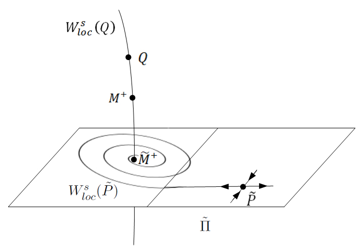
Refer to caption
Figure 9: The configuration of objects in Π~\tilde{\Pi} when M+∈Ws​(Q)M^{+}\in W^{s}(Q).

Proof of Lemma 7. Consider now a periodic orbit {Q=Q1(y1,x1,z1),Q2(y2,x2,z2),Q3(y3,\{Q=Q_{1}(y_{1},x_{1},z_{1}),Q_{2}(y_{2},x_{2},z_{2}),Q_{3}(y_{3}, x3,x_{3}, z3)}z_{3})\} of period 3. We will show that there exist parameter values for which Q1Q_{1} has index 2, and the point M+M^{+} lies on the local stable manifold Wl​o​cs​(Q1)W^{s}_{loc}(Q_{1}) (figure 9).

Refer to caption
Figure 10: The configurations of points Q1~,\tilde{Q_{1}}, Q2~\tilde{Q_{2}} and Q3~\tilde{Q_{3}} on the quotient cross-section Π~\tilde{\Pi}.

Depending on the sign of μ\mu and the values of θ1−θ\theta_{1}-\theta, there are four logical possibilities of configurations of the points Q1,Q2Q_{1},Q_{2} and Q3Q_{3} on Π\Pi, (see figure 10), which are given by

1.Q1=T2(Q3)∈Π1,Q2=T1(Q1)∈Π1,Q3=T1(Q2)∈Π2;2.Q1=T2(Q3)∈Π1,Q2=T1(Q1)∈Π2,Q3=T2(Q2)∈Π2,3.Q1=T2(Q3)∈Π2,Q2=T2(Q1)∈Π1,Q3=T1(Q2)∈Π2;4.Q1=T2(Q3)∈Π2,Q2=T2(Q1)∈Π2,Q3=T2(Q2)∈Π2.\begin{array}[]{ll}1.&Q_{1}=T_{2}(Q_{3})\in\Pi_{1}\,,\quad Q_{2}=T_{1}(Q_{1})\in\Pi_{1}\,,\quad Q_{3}=T_{1}(Q_{2})\in\Pi_{2}\,;\\[5.0pt] 2.&Q_{1}=T_{2}(Q_{3})\in\Pi_{1}\,,\quad Q_{2}=T_{1}(Q_{1})\in\Pi_{2}\,,\quad Q_{3}=T_{2}(Q_{2})\in\Pi_{2}\,,\\[5.0pt] 3.&Q_{1}=T_{2}(Q_{3})\in\Pi_{2}\,,\quad Q_{2}=T_{2}(Q_{1})\in\Pi_{1}\,,\quad Q_{3}=T_{1}(Q_{2})\in\Pi_{2}\,;\\[5.0pt] 4.&Q_{1}=T_{2}(Q_{3})\in\Pi_{2}\,,\quad Q_{2}=T_{2}(Q_{1})\in\Pi_{2}\,,\quad Q_{3}=T_{2}(Q_{2})\in\Pi_{2}\,.\\[5.0pt] \end{array} (62)

Note that, for different configuration, the formulas for the parameters uu and vv will change but the same result in Lemma 7 holds.

Here we only consider the case where μ<0\mu<0 and (θ1−θ)∈(0,π2](\theta_{1}-\theta)\in(0,\dfrac{\pi}{2}], i.e. the fourth configuration in (62).

We first need a formula for the local stable manifold Wl​o​cs​(Q1)W^{s}_{loc}(Q_{1}), which is a leaf of the strong-stable foliation ℱ1\mathcal{F}_{1}. The leaves of ℱ1\mathcal{F}_{1} are given by the following lemma.

Lemma 8.

Let M⁡(y0,x0,z0)M(y_{0},x_{0},z_{0}) be a point on Π\Pi with y0y_{0} sufficiently small. The local strong stable manifold Wl​o​cs​s​(M)W^{ss}_{loc}(M) (i.e. the leaf of ℱ1\mathcal{F}_{1} through MM) is the graph of the function

(y,x)=(y0+(z−z0)​a1,x0+(z−z0)​a2),(y,x)=(y_{0}+(z-z_{0})a_{1},\,\,x_{0}+(z-z_{0})a_{2})\,,

where a1=o⁡(|y0|)a_{1}=o(|y_{0}|) and a2=o​(1)y0→0a_{2}=o(1)_{y_{0}\to 0} are (n−3)(n-3)-dimensional vectors whose components are certain functions of y0,x0,z0y_{0},x_{0},z_{0} and the parameters ε\varepsilon satisfying

∂i+k+l+no⁡(|y0|)∂iy0​∂kx0​∂lz0​∂nε\displaystyle\dfrac{\partial^{i+k+l+n}o(|y_{0}|)}{\partial^{i}y_{0}\,\partial^{k}x_{0}\,\partial^{l}z_{0}\,\partial^{n}\varepsilon} =o⁡(|y0|1−i)i+k+l+n⩽(r−1),\displaystyle=o(|y_{0}|^{1-i})\quad i+k+l+n\leqslant(r-1)\,,
∂k+l+no⁡(1)∂kx0​∂lz0​∂nε\displaystyle\dfrac{\partial^{k+l+n}o(1)}{\partial^{k}x_{0}\,\partial^{l}z_{0}\,\partial^{n}\varepsilon} =o​(1)y0→0k+l+n⩽(r−1).\displaystyle=o(1)_{y_{0}\to 0}\quad k+l+n\leqslant(r-1)\,.

This result is lemma 4 in [16] and we omit the proof here. The local stable manifold Wl​o​cs​(Q1)W^{s}_{loc}(Q_{1}) is now given by

y=y1+(z−z1)​δ1,x=x1+(z−z1)​δ2,\begin{array}[]{rcl}y&=&y_{1}+(z-z_{1})\delta_{1}\,,\\[7.0pt] x&=&x_{1}+(z-z_{1})\delta_{2}\,,\end{array} (63)

where δ1=(o⁡(|y1|),⋯,o⁡(|y1|))T\delta_{1}=(o(|y_{1}|),\cdots,o(|y_{1}|))^{T}, δ2=(O⁡(|y1|α),…,O⁡(|y1|α))T\delta_{2}=(O(|y_{1}|^{\alpha}),\dots,O(|y_{1}|^{\alpha}))^{T} and α\alpha is determined by the spectrum gap between the week stable eigenvalue and the first strong stable eigenvalue (i.e. −λ±ω​i-\lambda\pm\omega i and α1\alpha_{1} for the system XX mentioned in the beginning of this paper).

Recall the transformation (19) for the yy-coordinate of a point on Π2\Pi_{2}:

ω​ln⁡1|y|=2​π​j+ξ−θ,ξ∈[0,2​π).\omega\ln\dfrac{1}{|y|}=2\pi j+\xi-\theta\,,\quad\xi\in[0,2\pi)\,.

By the formula (57) of the map T2T_{2} , the formula (63) for Wl​o​cs​(Q1)W^{s}_{loc}(Q_{1}), and Lemma 3 (index-2 condition), finding a periodic orbit {Q1,Q2,Q3}\{Q_{1},Q_{2},Q_{3}\} of period 3 and index 2 with the property M+∈Ws​(Q1)M^{+}\in W^{s}(Q_{1}) is equivalent to solve the following system of equations:

y1=−μ−Bx3|y3|ρcosξ3+o(|y3|ρ),\displaystyle y_{1}=-\mu-Bx_{3}|y_{3}|^{\rho}\cos\xi_{3}+o(|y_{3}|^{\rho})\,,
x1=1+ζ+B1​x3​|y3|ρ​cos⁡(ξ3+θ1−θ)+o⁡(|y3|ρ),\displaystyle x_{1}=1+\zeta+B_{1}x_{3}|y_{3}|^{\rho}\cos(\xi_{3}+\theta_{1}-\theta)+o(|y_{3}|^{\rho})\,,
z1=z−+(B2​x3​|y3|ρ​cos⁡(ξ3+θ2−θ)+o⁡(|y3|ρ)⋯Bn−2​x3​|y3|ρ​cos⁡(ξ3+θn−2−θ)+o⁡(|y3|ρ)),\displaystyle z_{1}=z^{-}+\begin{pmatrix}B_{2}x_{3}|y_{3}|^{\rho}\cos{(\xi_{3}+\theta_{2}-\theta)}+o(|y_{3}|^{\rho})\\ \cdots\\ B_{n-2}x_{3}|y_{3}|^{\rho}\cos(\xi_{3}+\theta_{n-2}-\theta)+o(|y_{3}|^{\rho})\end{pmatrix}\,,
y2=−μ−Bx1|y1|ρcosξ3+o(|y1|ρ),\displaystyle y_{2}=-\mu-Bx_{1}|y_{1}|^{\rho}\cos\xi_{3}+o(|y_{1}|^{\rho})\,,
x2=1+ζ+B1​x1​|y1|ρ​cos⁡(ξ1+θ1−θ)+o⁡(|y1|ρ),\displaystyle x_{2}=1+\zeta+B_{1}x_{1}|y_{1}|^{\rho}\cos(\xi_{1}+\theta_{1}-\theta)+o(|y_{1}|^{\rho})\,,
z2=z−+(B2​x1​|y1|ρ​cos⁡(ξ1+θ2−θ)+o⁡(|y1|ρ)⋯Bn−2​x1​|y1|ρ​cos⁡(ξ3+θn−2−θ)+o⁡(|y1|ρ)),\displaystyle z_{2}=z^{-}+\begin{pmatrix}B_{2}x_{1}|y_{1}|^{\rho}\cos{(\xi_{1}+\theta_{2}-\theta)}+o(|y_{1}|^{\rho})\\ \cdots\\ B_{n-2}x_{1}|y_{1}|^{\rho}\cos(\xi_{3}+\theta_{n-2}-\theta)+o(|y_{1}|^{\rho})\end{pmatrix}\,,
y3=−μ−Bx2|y2|ρcosξ2+o(|y2|ρ),\displaystyle y_{3}=-\mu-Bx_{2}|y_{2}|^{\rho}\cos\xi_{2}+o(|y_{2}|^{\rho})\,,
x3=1+ζ+B1​x2​|y2|ρ​cos⁡(ξ2+θ1−θ)+o⁡(|y2|ρ),\displaystyle x_{3}=1+\zeta+B_{1}x_{2}|y_{2}|^{\rho}\cos(\xi_{2}+\theta_{1}-\theta)+o(|y_{2}|^{\rho})\,,
z3=z−+(B2​x2​|y2|ρ​cos⁡(ξ2+θ2−θ)+o⁡(|y2|ρ)⋯Bn−2​x2​|y2|ρ​cos⁡(ξ2+θn−2−θ)+o⁡(|y2|ρ)),\displaystyle z_{3}=z^{-}+\begin{pmatrix}B_{2}x_{2}|y_{2}|^{\rho}\cos{(\xi_{2}+\theta_{2}-\theta)}+o(|y_{2}|^{\rho})\\ \cdots\\ B_{n-2}x_{2}|y_{2}|^{\rho}\cos(\xi_{2}+\theta_{n-2}-\theta)+o(|y_{2}|^{\rho})\end{pmatrix}\,,
μ=y1+δ1​(z+−z1),\displaystyle\mu=y_{1}+\delta_{1}(z^{+}-z_{1})\,,
1=x1+δ2​(z+−z1),\displaystyle 1=x_{1}+\delta_{2}(z^{+}-z_{1})\,,
cos⁡(ξ1−φ)​cos⁡(ξ2−φ)​cos⁡(ξ3−φ)=c​ψ,\displaystyle\cos(\xi_{1}-\varphi)\cos(\xi_{2}-\varphi)\cos(\xi_{3}-\varphi)=c\psi\,,

where the first nine equations give us a periodic orbit of period 3, the next two equations imply Ws​s​(Q)∩M+≠∅W^{ss}(Q)\cap M^{+}\neq\emptyset, and the last one makes this orbit having index 2. After expressing xx and zz as functions of yy, we can drop the equations for them (except the one for x1x_{1} used to obtain M+∈Ws​(Q1)M^{+}\in W^{s}(Q_{1})). The reduced system assumes the form

y1=−μ−Bnew|y3|ρcosξ3+o(|y3|ρ)+O(|y|2ρ|y|3ρ)+O(|y|1ρ|y|2ρ|y|3ρ),\displaystyle y_{1}=-\mu-B_{\mbox{new}}|y_{3}|^{\rho}\cos\xi_{3}+o(|y_{3}|^{\rho})+O(|y|_{2}^{\rho}|y|_{3}^{\rho})+O(|y|_{1}^{\rho}|y|_{2}^{\rho}|y|_{3}^{\rho})\,, (64)
y2=−μ−Bnew|y1|ρcosξ1+o(|y1|ρ)+O(|y|1ρ|y|3ρ)+O(|y|1ρ|y|2ρ|y|3ρ),\displaystyle y_{2}=-\mu-B_{\mbox{new}}|y_{1}|^{\rho}\cos\xi_{1}+o(|y_{1}|^{\rho})+O(|y|_{1}^{\rho}|y|_{3}^{\rho})+O(|y|_{1}^{\rho}|y|_{2}^{\rho}|y|_{3}^{\rho})\,, (65)
y3=−μ−Bnew|y2|ρcosξ2+o(|y2|ρ)+O(|y|1ρ|y|2ρ)+O(|y|1ρ|y|2ρ|y|3ρ),\displaystyle y_{3}=-\mu-B_{\mbox{new}}|y_{2}|^{\rho}\cos\xi_{2}+o(|y_{2}|^{\rho})+O(|y|_{1}^{\rho}|y|_{2}^{\rho})+O(|y|_{1}^{\rho}|y|_{2}^{\rho}|y|_{3}^{\rho})\,, (66)
x1=1+ζ+B1​|y3|ρ​cos⁡(ξ3+θ1−θ)+o⁡(|y3|ρ),\displaystyle x_{1}=1+\zeta+B_{1}|y_{3}|^{\rho}\cos(\xi_{3}+\theta_{1}-\theta)+o(|y_{3}|^{\rho})\,, (67)
μ=y1+δ1​(z+−z1),\displaystyle\mu=y_{1}+\delta_{1}(z^{+}-z_{1})\,, (68)
1=x1+δ2​(z+−z1),\displaystyle 1=x_{1}+\delta_{2}(z^{+}-z_{1})\,, (69)
cos⁡(ξ1−φ)​cos⁡(ξ2−φ)​cos⁡(ξ3−φ)=c​ψ,\displaystyle\cos(\xi_{1}-\varphi)\cos(\xi_{2}-\varphi)\cos(\xi_{3}-\varphi)=c\psi\,, (70)

where Bnew=(1+ζ)​BB_{\mbox{new}}=(1+\zeta)B and we drop the subscript for simplicity. We now impose two relations among y1,y2y_{1},y_{2} and y3y_{3} which are

|y3|ρ∼|y1|and|y1|ρ∼|y2|.|y_{3}|^{\rho}\sim|y_{1}|\quad\mbox{and}\quad|y_{1}|^{\rho}\sim|y_{2}|. (71)

It can be seen later that these relations agree with the solutions to above system of equations. Therefore, we replace the last three terms in each of equations (64) - (66) by o⁡(|y3|ρ)o(|y_{3}|^{\rho}), o⁡(|y1|ρ)o(|y_{1}|^{\rho}) and o⁡(|y2|ρ)o(|y_{2}|^{\rho}), respectively.

From now on, we will denote by dots the small terms which tend to zero as j1,j2,j3→+∞j_{1},j_{2},j_{3}\to+\infty. By plugging equation (69) into (67) and letting

ζ=−δ2​(z+−z1),\zeta=-\delta_{2}(z^{+}-z_{1})\,, (72)

we have

B1​|y3|ρ​cos⁡(ξ3+θ1−θ)+o⁡(|y3|ρ)=0,B_{1}|y_{3}|^{\rho}\cos(\xi_{3}+\theta_{1}-\theta)+o(|y_{3}|^{\rho})=0\,, (73)

which, by dividing |y3|ρ|y_{3}|^{\rho} on both sides, gives

B1​cos⁡(ξ3+θ1−θ)+o​(1)y3→0=0.B_{1}\cos(\xi_{3}+\theta_{1}-\theta)+o(1)_{y_{3}\to 0}=0\,. (74)

This implies

ξ3=π2+k​π−θ1+θ+…andcos⁡ξ3=sin⁡(θ1−θ)+….\xi_{3}=\dfrac{\pi}{2}+k\pi-\theta_{1}+\theta+...\quad\mbox{and}\quad\cos{\xi_{3}}=\sin(\theta_{1}-\theta)+...\,. (75)

Note that, to obtain (74), we only need ζ+δ2​(z+−z1)∼o⁡(|y3|ρ)\zeta+\delta_{2}(z^{+}-z_{1})\sim o(|y_{3}|^{\rho}). Recall the assumption at the beginning of the proof that (θ1−θ)∈(0,π2](\theta_{1}-\theta)\in(0,\dfrac{\pi}{2}]. We have k=0k=0 by noting ξ3∈[0,2​π)\xi_{3}\in[0,2\pi). We remark here that the relation |y3|ρ∼|y1||y_{3}|^{\rho}\sim|y_{1}| can now be obtained by plugging (68) and (75) into (64), which is one of the relations 71 we assumed before.

By using the relations given by (71) and plugging equation (68) into (64) - (66), we get

y1=−y1−B|y3|ρcosξ3+o(|y3|ρ),\displaystyle y_{1}=-y_{1}-B|y_{3}|^{\rho}\cos\xi_{3}+o(|y_{3}|^{\rho})\,, (76)
y2=−y1−B|y1|ρcosξ1+o(|y1|ρ),\displaystyle y_{2}=-y_{1}-B|y_{1}|^{\rho}\cos\xi_{1}+o(|y_{1}|^{\rho})\,, (77)
y3=−y1−B|y2|ρcosξ2+o(|y2|ρ).\displaystyle y_{3}=-y_{1}-B|y_{2}|^{\rho}\cos\xi_{2}+o(|y_{2}|^{\rho})\,. (78)

By plugging equation (75) into (76), we further obtain

y1=−12​B​|y3|ρ​sin⁡(θ1−θ)+o⁡(|y3ρ|).y_{1}=-\frac{1}{2}B|y_{3}|^{\rho}\sin(\theta_{1}-\theta)+o(|y_{3}^{\rho}|)\,. (79)

We now apply the transformation (19) to equations (79), (77) and (78), and obtain

exp⁡(−2​π​j1−ξ1+θω)=12​B​exp​((−2​π​j3−ξ3+θ)​ρω)​sin⁡σ+o⁡(exp⁡(−2​π​ρ​j3ω)),\displaystyle\quad\mathrm{exp}\bigg(\dfrac{-2\pi j_{1}-\xi_{1}+\theta}{\omega}\bigg)=\frac{1}{2}B\mathrm{exp}\bigg(\dfrac{(-2\pi j_{3}-\xi_{3}+\theta)\rho}{\omega}\bigg)\sin{\sigma}+o\bigg(\mathrm{exp}\bigg(\dfrac{-2\pi\rho j_{3}}{\omega}\bigg)\bigg)\,, (80)
−exp(−2​π​j2−ξ2+θω)=exp(−2​π​j1−ξ1+θω)−Bexp((−2​π​j1−ξ1+θ)​ρω)cosξ1\displaystyle-\mathrm{exp}\bigg(\dfrac{-2\pi j_{2}-\xi_{2}+\theta}{\omega}\bigg)=\mathrm{exp}\bigg(\dfrac{-2\pi j_{1}-\xi_{1}+\theta}{\omega}\bigg)-B\mathrm{exp}\bigg(\dfrac{(-2\pi j_{1}-\xi_{1}+\theta)\rho}{\omega}\bigg)\cos{\xi_{1}}
+o⁡(exp⁡(−2​π​ρ​j1ω)),\displaystyle\qquad\qquad\qquad\qquad\qquad\qquad+o\bigg(\mathrm{exp}\bigg(\dfrac{-2\pi\rho j_{1}}{\omega}\bigg)\bigg)\,, (81)
−exp(−2​π​j3−ξ3+θω)=exp(−2​π​j1−ξ1+θω)−Bexp((−2​π​j2−ξ2+θ)​ρω)cosξ2\displaystyle-\mathrm{exp}\bigg(\dfrac{-2\pi j_{3}-\xi_{3}+\theta}{\omega}\bigg)=\mathrm{exp}\bigg(\dfrac{-2\pi j_{1}-\xi_{1}+\theta}{\omega}\bigg)-B\mathrm{exp}\bigg(\dfrac{(-2\pi j_{2}-\xi_{2}+\theta)\rho}{\omega}\bigg)\cos{\xi_{2}}
+o⁡(exp⁡(−2​π​ρ​j2ω)).\displaystyle\qquad\qquad\qquad\qquad\qquad\qquad+o\bigg(\mathrm{exp}\bigg(\dfrac{-2\pi\rho j_{2}}{\omega}\bigg)\bigg)\,. (82)

Let us solve those equations for sufficiently large j1,j2j_{1},j_{2} and j3j_{3}.

We first divide equation (80) by o⁡(exp⁡(−2​π​ρ​j3ω))o\big(\mathrm{exp}\big(\dfrac{-2\pi\rho j_{3}}{\omega}\big)\big) on both sides, and then take j3j_{3} large enough. After taking logarithm on both sides of the resulting equation, we obtain

ρ​j3−j1=12​π​(ω​log⁡(12​B​sin⁡σ)−θ+ρ​θ−ρ​ξ3+ξ1)+….\rho j_{3}-j_{1}=\frac{1}{2\pi}\big(\omega\log{\big(\frac{1}{2}B\sin{\sigma}\big)}-\theta+\rho\theta-\rho\xi_{3}+\xi_{1}\big)+\ldots\,. (83)

In a similar way, equation (81) gives

cos⁡ξ1=B−1​exp​(2​π​(ρ​j1−j2)ω)​exp​(θ−ρ​θ+ρ​ξ1−ξ2ω)+….\cos{\xi_{1}}=B^{-1}\mathrm{exp}\bigg(\dfrac{2\pi(\rho j_{1}-j_{2})}{\omega}\bigg)\mathrm{exp}\bigg(\dfrac{\theta-\rho\theta+\rho\xi_{1}-\xi_{2}}{\omega}\bigg)+\ldots\,. (84)

By moving the first term on the RHS of (82) to its LHS, multiplying −1-1 on both sides, and then taking logarithm, we have

log(exp(−2​π​j3−ξ3+θω)+exp(−2​π​j1−ξ1+θω))=log(Bexp((−2​π​j2−ξ2+θ)​ρω)cosξ2+⋯),\log{\bigg(\mathrm{exp}\bigg(\dfrac{-2\pi j_{3}-\xi_{3}+\theta}{\omega}\bigg)+\mathrm{exp}\bigg(\dfrac{-2\pi j_{1}-\xi_{1}+\theta}{\omega}\bigg)\bigg)}=\log{\bigg(B\mathrm{exp}\bigg(\dfrac{(-2\pi j_{2}-\xi_{2}+\theta)\rho}{\omega}\bigg)\cos{\xi_{2}}+\cdots\bigg)}\,,\\ (85)

i.e.

−2​π​j1−ξ1+θω+log(1+exp(−2​π​(j3−j1)−ξ3+ξ1ω)=log(Bexp((−2​π​j2−ξ2+θ)​ρω)cosξ2+⋯).\dfrac{-2\pi j_{1}-\xi_{1}+\theta}{\omega}+\log\bigg(1+\mathrm{exp}\bigg(\dfrac{-2\pi(j_{3}-j_{1})-\xi_{3}+\xi_{1}}{\omega}\bigg)=\log{\bigg(B\mathrm{exp}\bigg(\dfrac{(-2\pi j_{2}-\xi_{2}+\theta)\rho}{\omega}\bigg)\cos{\xi_{2}}+\cdots\bigg)}\,. (86)

By noting j3≫j1j_{3}\gg j_{1} from the relation |y3|ρ∼|y1||y_{3}|^{\rho}\sim|y_{1}| stated in (71), the last equation implies

cos⁡ξ2=B−1​exp​(2​π​(ρ​j2−j1)ω)​exp​(θ−ρ​θ+ρ​ξ2−ξ1ω)+….\cos{\xi_{2}}=B^{-1}\mathrm{exp}\bigg(\dfrac{2\pi(\rho j_{2}-j_{1})}{\omega}\bigg)\mathrm{exp}\bigg(\dfrac{\theta-\rho\theta+\rho\xi_{2}-\xi_{1}}{\omega}\bigg)+\ldots\,. (87)

Let us now look into equation (70) of the index-2 condition. The equation (75) implies that cos⁡(ξ3−φ)\cos{(\xi_{3}-\varphi)} cannot be generically arbitrarily small. We show that cos⁡(ξ2−φ)\cos(\xi_{2}-\varphi) also cannot be arbitrarily small. Suppose cos⁡(ξ2−φ)=o​(1)j1,j2,j3→∞\cos(\xi_{2}-\varphi)=o(1)_{j_{1},j_{2},j_{3}\to\infty} and note that yiy_{i} are close to 0. Since cos⁡ξ2\cos\xi_{2} is finite and |y3|ρ∼|y1||y_{3}|^{\rho}\sim|y_{1}| (71), we have |y2|ρ∼|y1||y_{2}|^{\rho}\sim|y_{1}| from (78). This contradicts with our assumption that |y1|ρ∼|y2||y_{1}|^{\rho}\sim|y_{2}| (71). We now assume that cos⁡(ξ1−φ)=o​(1)j1,j2,j3→∞\cos{(\xi_{1}-\varphi)}=o(1)_{j_{1},j_{2},j_{3}\to\infty}, which leads to

ξ1=3​π2+φ+…andcos⁡ξ1=sin⁡φ+….\xi_{1}=\frac{3\pi}{2}+\varphi+\ldots\quad\mbox{and}\quad\cos{\xi_{1}}=\sin{\varphi}+\ldots\quad. (88)

We plug equation (88) into (84), and then get

ρj1−j2=12​π(ωlog(Bcosξ1)−θ+ρθ−ρξ1+ξ2)+….\rho j_{1}-j_{2}=\frac{1}{2\pi}\big(\omega\log{(B\cos{\xi_{1}})}-\theta+\rho\theta-\rho\xi_{1}+\xi_{2}\big)+\ldots\quad. (89)

Since j1,j2j_{1},j_{2} are large and the RHS of (89) is uniformly bounded, we have

ρ​j1∼j2,\rho j_{1}\sim j_{2}\,,

which agrees with the assumption that |y1|ρ∼|y2||y_{1}|^{\rho}\sim|y_{2}| (71). We can find ξ2\xi_{2} by plugging this into equation (87):

cos⁡ξ2=o​(1)j1,j2,j3→+∞andξ2=π2+…or3​π2+….\cos{\xi_{2}}=o(1)_{j_{1},j_{2},j_{3}\to+\infty}\quad\mbox{and}\quad\xi_{2}=\dfrac{\pi}{2}+\ldots\quad\text{or}\quad\dfrac{3\pi}{2}+\ldots\quad. (90)

For certainty, we let ξ2=π2+⋯\xi_{2}=\dfrac{\pi}{2}+\cdots. We now rewrite (89) and (83) with values of ξi\xi_{i} as

ρ​j1−j2=12​π​(ω​log⁡(B​sin⁡φ)−θ+ρ​θ−ρ⁡(3​π2+φ)+π2)+…=:u+…,\rho j_{1}-j_{2}=\frac{1}{2\pi}\bigg(\omega\log{(B\sin{\varphi})}-\theta+\rho\theta-\rho\bigg(\frac{3\pi}{2}+\varphi\bigg)+\frac{\pi}{2}\bigg)+\ldots=:u+\ldots\,, (91)

and

ρ​j3−j1=12​π​(ω​log⁡(12​B​sin⁡(θ1−θ))−θ+ρ​θ−ρ⁡(π2+θ−θ1)+3​π2+φ)+…=:v+….\rho j_{3}-j_{1}=\frac{1}{2\pi}\bigg(\omega\log{\bigg(\frac{1}{2}B\sin{(\theta_{1}-\theta)}\bigg)}-\theta+\rho\theta-\rho\bigg(\frac{\pi}{2}+\theta-\theta_{1}\bigg)+\frac{3\pi}{2}+\varphi\bigg)+\ldots=:v+\ldots\,. (92)

Equations (91) and (92) are relations among parameters. If we can find integers j1,j2j_{1},j_{2} and j3j_{3} such that the parameters satisfy the these two relations, then the system of equations (64) - (70) can be solved. In fact, for any given NN, we need (91) and (92) to be satisfied with some (j1,j2,j3)(j_{1},j_{2},j_{3}) where ji>Nj_{i}>N (i=1,2,3)(i=1,2,3). This is because we need jij_{i} to be sufficiently large so that the terms denoted by dots can be sufficiently small when we take the limit ji→+∞j_{i}\to+\infty.

Now recall the parameter values of ρ,u\rho,u and vv stated in Lemma 7, which are

ρ^=pq,u^=p1q,v^=p2q,\hat{\rho}=\frac{p}{q}\,,\hat{u}=\frac{p_{1}}{q}\,,\hat{v}=\frac{p_{2}}{q}\,, (93)

where p,qp,q are co-prime integers and p1,p2p_{1},p_{2} are any integers. We now show that there exists a sequence {(j1i,j2i,j3i)}\{(j_{1}^{i},j_{2}^{i},j_{3}^{i})\} of triples of integers where j1i,j2i,j3i→+∞j_{1}^{i},j_{2}^{i},j_{3}^{i}\to+\infty as i→+∞i\to+\infty such that, for each triple (j1i,j2i,j3i)(j_{1}^{i},j_{2}^{i},j_{3}^{i}), the corresponding parameter values ui,viu_{i},v_{i} obtained from the relations (91) and (92) with ρ=ρ^\rho=\hat{\rho} satisfy that ui→u^u_{i}\to\hat{u} and vi→v^v_{i}\to\hat{v} as i→+∞i\to+\infty. Finding such sequence {(j1i,j2i,j3i)}\{(j_{1}^{i},j_{2}^{i},j_{3}^{i})\} is equivalent to seeking for integer solutions (j1i,j2i,j3i)(j_{1}^{i},j_{2}^{i},j_{3}^{i}) with j1i,j2i,j3i→+∞j_{1}^{i},j_{2}^{i},j_{3}^{i}\to+\infty as i→+∞i\to+\infty to the following system of equations:

{ρ^​j1−j2=u^,ρ^​j3−j1=v^.\left\{\begin{array}[]{rcl}\hat{\rho}j_{1}-j_{2}&=&\hat{u}\,,\\[5.0pt] \hat{\rho}j_{3}-j_{1}&=&\hat{v}\,.\end{array}\right. (94)

By plugging the relations (93) into (94), we get a system of two linear Diophantine equations:

{p​j1−q​j2=p1,p​j3−q​j1=p2.\left\{\begin{array}[]{rcl}pj_{1}-qj_{2}&=&p_{1}\,,\\[5.0pt] pj_{3}-qj_{1}&=&p_{2}\,.\end{array}\right.\ (95)

Note that a linear Diophantine equation a​x+b​y=cax+by=c has integer solutions if and only if cc is a multiple of gcd⁡(a,b)\gcd(a,b). For a known solution (x,y)(x,y), we can construct infinitely many solutions of the form (x+k​v,y−k​u)(x+kv,y-ku), where u=ag​c​d​(a,b),v=bg​c​d​(a,b)u=\frac{a}{gcd(a,b)},v=\frac{b}{gcd(a,b)} and k=0,±1,±2​….k=0,\pm 1,\pm 2\ldots\,. It is obvious that if p,qp,q are co-prime, then the two equations in (95) can be solved separately. The solutions to the first equation are of the form (j^1+k​q,j^2+k​p)(\hat{j}_{1}+kq,\hat{j}_{2}+kp), where (j^1,j^2)(\hat{j}_{1},\hat{j}_{2}) is a solution to the first equation and kk is an arbitrary integer. Now let us plug j1=j^1+k​qj_{1}=\hat{j}_{1}+kq into the second equation of (95) and sort the terms. We have

p​j3−q2​k=n+q​j^1.pj_{3}-q^{2}k=n+q\hat{j}_{1}\,. (96)

Consider j3j_{3} and kk as unknowns. Note that p,q2p,q^{2} are co-prime since p,qp,q are co-prime. Thus, the solutions to (96) are of the form (j^3+i​q2,k^+i​p)(\hat{j}_{3}+iq^{2},\hat{k}+ip), where (j^3,k^)(\hat{j}_{3},\hat{k}) is a special solution to this equation and ii is an arbitrary integer. Therefore, we have infinitely many solutions (j1i,j2i,j3i)=(j^1+(k^+i​p)​q,j^2+(k^+i​p)​p,j^3+i​q2)(j^{i}_{1},j^{i}_{2},j^{i}_{3})=(\hat{j}_{1}+(\hat{k}+ip)q,\hat{j}_{2}+(\hat{k}+ip)p,\hat{j}_{3}+iq^{2}) to (95). Obviously, the integers j1i,j2ij^{i}_{1},j^{i}_{2} and j3ij^{i}_{3} can be simultaneously arbitrarily large. Hence, we find the desired sequence {(j1i,j2i,j3i)}\{(j_{1}^{i},j_{2}^{i},j_{3}^{i})\}.

For each triple (j1i,j2i,j3i)(j_{1}^{i},j_{2}^{i},j_{3}^{i}) with sufficiently large ii, the system of equations (64) - (70) can be solved. The corresponding parameter values μi\mu_{i} and ζi\zeta_{i} are obtained from equations (68) and (72), respectively. Lemma 7 is proved. ∎

3.2.4 Quasi-transverse intersection Ws​(Q)∩Wu​(P)W^{s}(Q)\cap W^{u}(P)

One can check, by iterating a vertical line connecting PP and a point in Π0\Pi_{0} like what we did in the proof of Theorem 1, that the unstable manifold of the index-1 fixed point P⁡(yp,xp,zp)P(y_{p},x_{p},z_{p}) is a spiral winding onto M+​(μ,1,z+)M^{+}(\mu,1,z^{+}), which is given by

y=μ+A​xp​tρ​cos⁡(ω​ln⁡(1t)+η)+o⁡(tρ),x=1+A1​xp​tρ​cos⁡(ω​ln⁡(1t)+η1)+o⁡(tρ),z=z++(A2​xp​tρ​cos⁡(ω​ln⁡1t+η2)+o⁡(tρ)⋯An−2​xp​tρ​cos⁡(ω​ln⁡1t+ηn−2)+o⁡(tρ)),\begin{array}[]{rcl}y&=&\mu+Ax_{p}t^{\rho}\cos(\omega\ln(\dfrac{1}{t})+\eta)+o(t^{\rho})\,,\\[7.0pt] x&=&1+A_{1}x_{p}t^{\rho}\cos(\omega\ln(\dfrac{1}{t})+\eta_{1})+o(t^{\rho})\,,\\[7.0pt] z&=&z^{+}+\begin{pmatrix}A_{2}x_{p}t^{\rho}\cos{(\omega\ln{\dfrac{1}{t}}+\eta_{2})}+o(t^{\rho})\\ \cdots\\ A_{n-2}x_{p}t^{\rho}\cos(\omega\ln{\dfrac{1}{t}}+\eta_{n-2})+o(t^{\rho})\end{pmatrix}\,,\end{array} (97)

where t∈(0,yp)t\in(0,y_{p}). We take a point QQ given by Lemma 7 at parameter values (μj,ζj,ρ∗CLOSE,(\mu_{j},\zeta_{j},\rho^{*}, OPENuj,vj)u_{j},v_{j}) with jj sufficiently large such that PP remains a saddle fixed point. It follows that the non-empty intersection Wu​(P)∩Ws​(Q)W^{u}(P)\cap W^{s}(Q) can be created by an arbitrary perturbation in ζ\zeta in system Xμj,ζj,ρ∗,uj,vjX_{\mu_{j},\zeta_{j},\rho^{*},u_{j},v_{j}}. Indeed, by changing ζ\zeta, one can change the distance corresponding to xx-coordinate between M+M^{+} and Wl​o​cs​(Q1)W^{s}_{loc}(Q_{1}) (see Figure 5 and equation (72)). Therefore, for each jj, one can find a sequence ζji\zeta_{j}^{i} such that Wu​(P)∩Ws​(Q)W^{u}(P)\cap W^{s}(Q) is non-empty in the system Xμj,ζji,ρ∗,uj,vjX_{\mu_{j},\zeta_{j}^{i},\rho^{*},u_{j},v_{j}}, where ζji→ζj\zeta_{j}^{i}\to\zeta_{j} as i→+∞i\to+\infty. Consequently, one can construct a new sequence {(μj,ζj,uj,vj)}\{(\mu_{j},\zeta_{j},u_{j},v_{j})\} such that system Xμj,ζj,ρ∗,uj,vjX_{\mu_{j},\zeta_{j},\rho^{*},u_{j},v_{j}} has the intersection Wu​(P)∩Ws​(Q)W^{u}(P)\cap W^{s}(Q). This intersection is quasi-transverse by the same argument used in the beginning of Section 3.1.4.

3.2.5 Transverse intersection Wu​(Q)∩Ws​(P)W^{u}(Q)\cap W^{s}(P)

We now prove that the point P∈{Pk+}P\in\{P^{+}_{k}\} given by Lemma 6 and the point QQ given by Lemma 7 also satisfy Wu​(Q)∩Ws​(P)≠∅W^{u}(Q)\cap W^{s}(P)\neq\emptyset. Specifically, we first fix the point QQ and then find the point PP by Lemma 6 with the μ\mu value corresponding to QQ.

We remark here that we only show the existence of the transverse intersection Wu​(Q)∩Ws​(P)W^{u}(Q)\cap W^{s}(P) for the case where μj<0\mu_{j}<0 (the μ\mu value corresponding to QQ) and (θ1−θ)∈(0,π2](\theta_{1}-\theta)\in(0,\dfrac{\pi}{2}] i.e. the fourth configuration shown in figure 10. One can easily check that the transverse intersection Wu​(Q)∩Ws​(P)W^{u}(Q)\cap W^{s}(P) exists in other cases as well.

Let QQ has orbit {Q=Q1,Q2,Q3}\{Q=Q_{1},Q_{2},Q_{3}\}. We take an arbitrarily small neighborhood UU of the point Q1Q_{1}. We claim that there exists some ii such that T2(i)​(U)T_{2}^{(i)}(U) intersects Π0\Pi_{0} transversely. Indeed, this can be achieved by applying the same argument used in the proof of Lemma 5. We remark here that although Lemma 5 is for the case where μ=0\mu=0, it also holds for small μ≠0\mu\neq 0. Indeed, the key step in the proof of Lemma 5 is to show that the orbit of the point Q1~\tilde{Q_{1}} (projection of the index-2 point along the a leaf of the foliation ℱ1\mathcal{F}_{1}) is inside of a region in Π~\tilde{\Pi} bounded by {x=1+δ}\{x=1+\delta\}, {x=1−δ}\{x=1-\delta\} and two pre-images of {y=0}\{y=0\} under T~\tilde{T}. In the case where μ≠0\mu\neq 0, the difference is that there are only finite pre-images of {y=0}\{y=0\} (the smaller the value of μ\mu is the more pre-images we get). However, there are always some pre-images have a finite distance to {y=0}\{y=0\} as long as μ\mu is not too large. This implies that we can still find the desired region that contains the orbit of Q~1\tilde{Q}_{1} by choosing {Q1,Q2,Q3}\{Q_{1},Q_{2},Q_{3}\} sufficiently close to Π0\Pi_{0} (i.e. taking jj sufficiently large in Lemma 7).

Let T2(i)​(U)T_{2}^{(i)}(U) be the first iterate which intersects Π0\Pi_{0} transversely. We have three cases depending on which point Q1Q_{1}, Q2Q_{2} or Q3Q_{3} is contained in T2(i)​(U)T_{2}^{(i)}(U).

If we have Q3∈T2(i)​(U)Q_{3}\in T_{2}^{(i)}(U), i.e. T2(i)​(Q1)=Q3T_{2}^{(i)}(Q_{1})=Q_{3}, then there exists a connected component l⊂(T2(i)​(U)∩Π2)l\subset(T_{2}^{(i)}(U)\cap\Pi_{2}) joining Q3Q_{3} and a point M∈Π0M\in\Pi_{0}. It follows that T2​(l)⊂T2(i+1)​(U)T_{2}(l)\subset T_{2}^{(i+1)}(U) is a connected component joining T2​(Q3)=Q1∈Π2T_{2}(Q_{3})=Q_{1}\in\Pi_{2} and T2​(M)=M−∈Π1T_{2}(M)=M^{-}\in\Pi_{1} since we assumed μj<0\mu_{j}<0. By Lemma 6, the local stable manifold Wl​o​cs​(P)W^{s}_{loc}(P) is a surface between {y=0}\{y=0\} and {y=|μj|}\{y=|\mu_{j}|\}. It follows that T2(i+1)​(U)∩Wl​o​cs​(P)≠∅T_{2}^{(i+1)}(U)\cap W^{s}_{loc}(P)\neq\emptyset, which implies that Wl​o​cu​(Q1)∩Wl​o​cs​(P)≠∅W^{u}_{loc}(Q_{1})\cap W^{s}_{loc}(P)\neq\emptyset.

Refer to caption
Figure 11: The configuration of corresponding objects in the quotient cross-section Π~\tilde{\Pi}. If T~2(i)​(Q~1)=Q~1\tilde{T}_{2}^{(i)}(\tilde{Q}_{1})=\tilde{Q}_{1} for some ii, then we have Wl​o​cs​(P~−)∩l≠∅W^{s}_{loc}({\tilde{P}^{-}})\cap l\neq\emptyset and Wl​o​cu​(P~−)∩Wl​o​cs​(P~)≠∅W^{u}_{loc}({\tilde{P}^{-}})\cap W^{s}_{loc}({\tilde{P}})\neq\emptyset

Let now T2(i)​(Q1)=Q1T_{2}^{(i)}(Q_{1})=Q_{1} and ll be the connected component joining Q1Q_{1} and a point in Π0\Pi_{0}. Note that we have y1∼μjy_{1}\sim\mu_{j} since M+∈Ws​(Q)M^{+}\in W^{s}(Q) (see (68)). By applying Lemma 6 to the set {Pk−}\{P^{-}_{k}\}, one can find a point P−∈{Pk−}P^{-}\in\{P^{-}_{k}\} such that P−P^{-} remains an index-1 fixed point at μ=μj\mu=\mu_{j}, and its local stable manifold Wl​o​cs​(P−)W^{s}_{loc}(P^{-}) intersects ll. This gives Ws​(P−)∩Wu​(Q1)≠∅W^{s}(P^{-})\cap W^{u}(Q_{1})\neq\emptyset. Since Wu​(P−)W^{u}(P^{-}) is a spiral winding onto M−∈Π1M^{-}\in\Pi_{1}, it must intersect the surface {y=−μj}⊂Π1\{y=-\mu_{j}\}\subset\Pi_{1}. Also by Lemma 6, one can find a point P∈{Pk+}P\in\{P^{+}_{k}\} that remains fixed at μ=μj\mu=\mu_{j} with a local stable manifold between {y=0}\{y=0\} and {y=|μj|}\{y=|\mu_{j}|\}. Hence, we have Wu​(P−)∩Ws​(P)≠∅W^{u}(P^{-})\cap W^{s}(P)\neq\emptyset (see figure 11), which further implies Wu​(Q1)∩Ws​(P)≠∅W^{u}(Q_{1})\cap W^{s}(P)\neq\emptyset. The same result holds if T2(i)​(Q1)=Q2T_{2}^{(i)}(Q_{1})=Q_{2}. Indeed, the relation |y1|ρ∼|y2||y_{1}|^{\rho}\sim|y_{2}| implies that |y1|≪|y2||y_{1}|\ll|y_{2}|, and, therefore, Wl​o​cs​(P−)W^{s}_{loc}(P^{-}) must intersect the connected component joining Q2Q_{2} and a point in Π0\Pi_{0}.

Thus, for each quadruple (μj,ζj,uj,vj)(\mu_{j},\zeta_{j},u_{j},v_{j}), the system Xμj,ζj,ρ^,uj,vjX_{\mu_{j},\zeta_{j},\hat{\rho},u_{j},v_{j}} has a heterodimensional cycle related to two periodic orbits of index 2 and index 3 which correspond to the periodic points PP and QQ of the map TT, respectively. Theorem 2 is proved.

We remark here that any point P′P^{\prime} from {Pk+}\{P^{+}_{k}\} which, under the perturbation, remains an index-1 fixed point and is homoclinically related to the point PP given by Lemma 6 gives an transverse intersection Ws​(P′)∩Wu​(Q)W^{s}(P^{\prime})\cap W^{u}(Q). The quasi-transverse intersection Ws​(Q)∩Wu​(P′)W^{s}(Q)\cap W^{u}(P^{\prime}) can be obtained by the same argument in Section 3.2.4. Therefore, such point P′P^{\prime} can also be used to create a heterodimensional cycle with the point QQ.

4 Discussion

In this paper, we have showed two mechanisms for the emergences of heterodimensional cycles near a pair of Shilnikov loops. The further research is to check whether those heterodimensional cycles are robust or there are robust cycles nearby. Ideally, One might be able to find a blender or its analogue near a pair of Shilnikov loops.

This also links to the application question: how to detect heterodimensional cycles? As we know that Shilnikov loop along is a simple criterion for chaos. Now a pair of such loops, provided the volume hyperbolicity and the non-coincidence condition (which are also reasonably easy to verify), gives a simple and practical criterion for the heterodimensional chaos (i.e. chaotic dynamics where saddles with different dimensions of unstable manifolds coexist and are connected).

Acknowledgement

The author is grateful to his scientific adviser Dmitry Turaev for setting this problem and useful discussions.

References

  • [1] Anosov, D. V.. Geodesic flows on closed Riemannian manifolds of negative curvature. Proc. Steklov Inst. Math., 90 (1967), 1–235.
  • [2] Afraimovich, V. S., Bykov, V. V. and Shilnikov, L. P.. On the structurally unstable attracting limit sets of Lorenz attractor type. Tran. Moscow Math. Soc., 2 (1983), 153-215.
  • [3] Bonatti, C. and Díaz, L. J.. Persistent transitive diffeomorphisms. Annals of Mathematics, 143(2) (1996), 357-396.
  • [4] Bonatti, C., Díaz, L. J. and Viana, M.. Dynamics Beyond Uniform Hyperbolicity. Springer, Berlin, Heidelberg, New York, 2000.
  • [5] Bonatti, C. and Díaz, L. J.. Robust heterodimensional cycles and C1-generic dynamics. J. Inst. Math. Jussieu 7, no. 3 (2008), 469-525.
  • [6] Bonatti, C. and Crovisier, S.. Center manifolds for partially hyperbolic sets without strong unstable connections. Journal of the Institute of Mathematics of Jussieu, available on CJO2015. doi:10.1017/S1474748015000055.
  • [7] Chawanya, T. and Ashwin, P.. A minimal system with a depth-two heteroclinic network. Dyn. Syst., 25 (2010), pp. 397–412.
  • [8] Dawson, S., Grebogi, C., Sauer, T. and Yorke, A.. Obstructions to shadowing when a Lyapunov exponent fluctuates about zero. Phys. Rev. Lett. 73, 1927 – Published 3 October 1994.
  • [9] Díaz, L. J. and Rocha, J.. Non-connected heterodimensional cycles: bifurcation and stability. Nonlinearity, 5 (1992), 1315-1341.
  • [10] Díaz, L. J.. Robust nonhyperbolic dynamics and heterodimensional cycles. Ergodic Theory and Dynamical Systems, 15 (1995), 291-315.
  • [11] Díaz, L. J.. Persistence of cycles and nonhyperbolic dynamics at the unfolding of heteroclinic bifurcations. Nonlinearity, 8 (1995), 693-715.
  • [12] ELeonsky, V. M ., Kulagin, N. E., Turaev, D. V. and Shilnikov, L. P.. On the classification of selflocalized states of electromagnetic field within nonlinear medium. Proceedings of the iv international workshop on nonlinear and turbulent processes in physics, volume 2 (1989), 235-238.
  • [13] Gaspard, P.. Generation of a countable set of homoclinic flows through bifurcation, Physics Letters A, Volume 97, Issues 1-2, 8 August 1983, 1-4.
  • [14] Gonchenko, S. V., Shilnikov, L. P. and Turaev, D. V.. On global bifurcations in three-dimensional diffeomorphisms leading to wild Lorenz-like attractors. Regular and Chaotic Dynamics, 14:1 (2009), 137.
  • [15] Homburg, A. J.. Global aspects of homoclinic bifurcations of vector fields, Mem. Amer. Math. Soc. 121 (1996), no. 578, viii+128.
  • [16] Li, D. and Turaev, D. V.. Existence of heterodimensional cycles near Shilnikov loops. Preprint. arXiv:1512.01280 [math.DS].
  • [17] Ovsyannikov, I. M. and Shilnikov, L. P.. On systems with a saddle-focus homoclinic curve. Sbornik: Mathematics 58 (2) (1987) 557-574.
  • [18] Ovsyannikov, I. M. and Shilnikov, L. P.. Systems with a homoclinic curve of multidimensional saddle-focus type, and spiral chaos. Math. USSR Sbornik, 73 (1992), 415-443.
  • [19] Shilnikov, L. P.. A case of the existence of a countable number of periodic motions (Point mapping proof of existence theorem showing neighborhood of trajectory which departs from and returns to saddle-point focus contains denumerable set of periodic motions). SOVIET MATHEMATICS 6 (1965), 163-166.
  • [20] Shilnikov, L. P.. On a Poincaré-Birkhoff problem. Sbornik: Mathematics 3 (3), 353-371.
  • [21] Shilnikov, L. P.. A contribution to the problem of the structure of an extended neighborhood of a rough equilibrium state of saddle-focus type. Sbornik: Mathematics 10 (1) (1970), 91-102.
  • [22] Shilnikov, L. P., Shilnikov, A. L., Turaev, D. V. and Chua, L. O.. Methods Of Qualitative Theory In Nonlinear Dynamics (Part I). World Sci.-Singapore, New Jersey, London, Hong Kong, 2001.
  • [23] Shilnikov, L. P., Shilnikov, A. L., Turaev, D. V. and Chua, L. O.. Methods Of Qualitative Theory In Nonlinear Dynamics (Part II). World Sci.-Singapore, New Jersey, London, Hong Kong, 2001.
  • [24] Shilnikov, L. P. and Turaev, D. V.. Superhomoclinic orbits and multi-pulse homoclinic loops in Hamiltonian systems with discrete symmetries, Regular and Chaotic Dynamics 2, No. 3/4 (1997), 126–138.
  • [25] Shashkov, M. V. and Turaev, D. V.. An Existence theorem of smooth nonlocal center manifolds for systems close to a system with a homoclinic loop. J. Nonlinear Sci. Vol. 9 (1999), 525-573.
  • [26] Turaev, D. V.. On dimension of non-local bifurcational problems, International Journal of Bifurcation and Chaos, 6(5) (1996), 919-948.
  • [27] Turaev, D. V.. Multi-pulse homoclinic loops in systems with a smooth first integral Ergodic Theory, Analysis and Efficient Simulation of Dynamical Systems ed B Fiedler (Berlin: Springer) pp 691–716.
  • [28] Turaev, D. V. and Shilnikov, L. P.. An example of a wild strange attractor. Sbornik. Math. 189(2) (1998), 291-314.