Power-efficiency-dissipation relations in linear thermodynamics
Abstract
We derive general relations between maximum power, maximum efficiency, and minimum dissipation regimes from linear irreversible thermodynamics. The relations simplify further in the presence of a particular symmetry of the Onsager matrix, which can be derived from detailed balance. The results are illustrated on a periodically driven system and a three terminal device subject to an external magnetic field.
pacs
05.70.Ln,05.70.Ce,84.60.RbI Introduction
Thermodynamic machines transform different forms of energy into one another. For such a machine, it would be of obvious interest to maximize the power and the efficiency , and to minimize the dissipation [1, 2, 3, 4, 5, 6, 7, 8, 9, 10, 11, 12, 13, 14, 15, 16, 17, 18, 19, 20, 21, 22, 23, 24, 25, 26, 27, 28, 29, 30, 31, 32, 33, 34, 35, 36, 37]. The extrema (maximum or minimum) here are understood with respect to a variation of the engine’s load parameters, which are often the ones that are easy to tune. In general, the above goals are incompatible. For example, the efficiency when operating at maximum power is (in a time-symmetric setting) limited to half of the reversible efficiency . The latter efficiency, being an overall upper bound, can only be reached when operating reversibly, hence infinitely slowly. Consequently, the corresponding power vanishes. More generally, one may wonder whether there exist specific relationships between the regimes of maximum power (which will be denoted by a subscript ), maximum efficiency (subscript ) and minimum dissipation (subscript ).
Recently, such relations have been discovered between and in the context of two case studies [23, 36].
In this letter, we derive general relations between the three regimes, within the framework of linear irreversible thermodynamics. Two results stand out. The first one is a remarkably simple relation linking to :
| (1) |
As an implication note that, since power output and efficiency are positive, the efficiency at maximum power is at least half the maximum efficiency, . The second result links the regimes of and by two equally simple equations:
| (2) | |||||
| (3) |
where is the reference temperature of the system.
As a consequence, note that when minimum dissipation coincides with reversible operation, i.e., and , one finds from Eqs. (2,3) that .
The above relations become more specific when the Onsager matrix, which links the thermodynamic fluxes and forces, satisfies a generalized Onsager symmetry condition, which we discuss in more detail below. The ”standard” Onsager symmetry, which applies to time-symmetric machines, is a particular case. Under this extra condition, the link between maximum power and efficiency, cf. Eq. (1), splits into two separate relations, in agreement with the special cases discussed in [23, 36]:
| (4) |
To mention some further implications of these results, reversible efficiency, can only be reached when the power goes to zero, . Furthermore, implies , as first noted in [1] (for a symmetric Onsager matrix).
Note also that the equality sign in is only reached for , hence , illustrating the conflict between maximizing efficiency and maximizing power.
Under the same generalized Onsager symmetry condition, the links between maximum power and minimum dissipation, Eqs. (2,3), simplify as follows 11
1
Eq. (49) from [36] is identical to the second part of our Eq. (5) provided one identifies
the ’idle heat flux’ with our minimal dissipation .:
| (5) |
Zero minimum dissipation (with ) implies
and
Note the close interconnection between the results Eqs. (4,5), since all of them follow from Eqs. (1-3), if any one of them is valid.
We close the introduction with an important comment concerning the mathematical and physical content of the above relations. We will derive the above results first in the simple setting of two thermodynamic fluxes and forces, linked by a two-by-two Onsager matrix . The relations Eqs. (1-3) follow from straightforward algebra applied to the standard expressions from linear irreversible thermodynamics. No additional assumptions are needed. Eqs. (4,5) on the other hand require Onsager symmetry or anti-symmetry 22
2
Onsager anti-symmetry is defined by for all , i.e., . We next will show that both sets of results remain valid when the thermodynamic driving and loading force and flux are vectorial, i.e., they are composed of sub-forces and sub-fluxes, provided one performs the ”full” optimization, i.e., with respect to all the components of the loading force. The validity of Eqs. (4,5) then rests in addition on a generalized Onsager symmetry, (T standing for the transpose) or . This property can be derived from time-reversibility and detailed balance of the underlying micro-dynamics, and is therefore expected to have a very wide range of validity. We will illustrate this state of affairs on a system subject to a time-asymmetric periodic driving and a three-terminal device with an external magnetic field.
II Linear irreversible thermodynamics
The thermodynamic processes that drive machines are generally induced by a spatial or temporal variation in quantities such as (inverse) temperature, chemical potential, pressure, etc. These differences are responsible for so-called thermodynamic forces, which we will denote by . With every thermodynamic force, one can associate a flux, for example a heat flux or a particle flux, denoted as . The generic function of a machine is to transform one type of energy into another one. The simplest such construction thus features two forces, one playing the role of load force, say , and another functioning as driving force, . With proper definitions of fluxes and forces, the entropy production or dissipation, can be written as a bilinear form [40, 41]:
| (6) |
The working regime is defined as a driving entropy producing flux, say with , generating another flux against its own thermodynamic force . The standard example is that of a thermal machine, where a downhill heat flux pushes particles up a potential. The quantities of interest are the net dissipation , given in (6), the power output , which we define as 33 3 The temperature of the power producing device is the natural choice for the multiplicative factor . We however stress that the results Eqs. (1-5) are valid, irrespective of the choice of this temperature.
| (7) |
and the efficiency ,
| (8) |
The power output and efficiency are both positive by definition of the working regime. In addition, the second law implies that, in the working regime, , with the reversible limit reached for zero entropy production . Hence, one has:
| (9) |
Finally, by their definitions, power, efficiency and entropy production are not independent quantities but obey the following relation:
| (10) |
Focusing on the regime of linear irreversible thermodynamics, one assumes that the thermodynamics forces are small, so that the associated thermodynamic fluxes are linear in the forces:
| (11) |
The coefficients are known as the Onsager coefficients.
For a given thermodynamic process, one can consider its time-inverse, denoted by a tilde. It is obtained by reversing the time dependencies and inverting the variables, such as speed and magnetic field, which are odd under time-inversion. The above coefficients satisfy the so-called Onsager Casimir symmetry
[43]. This relation is particularly useful in the time-symmetric scenario with even variables, for which it reduces to the celebrated Onsager symmetry,
[44, 45].
We are now ready to calculate the values of the three key quantities, power, efficiency and dissipation, when performing the extremum of one of them with respect to the loading force . In calculating the maximum efficiency and power, we will assume to be in the working regime. This leads to nine expressions , of which, in view of Eq. (10), six are a-priori independent. Straightforward algebra leads to the following explicit expressions:
| (12) |
| (13) |
| (14) |
| (15) |
The surprise is that there are, in fact, only three independent quantities: one verifies by inspection the validity of the relations Eqs. (1-3). In the case of Onsager symmetry or anti-symmetry, these equations further simplify with the appearance of one additional relation, cf. Eqs. (4,5). Hence, we are left with only two independent quantities out of the original nine, for example any pair of power and efficiency, and , and , etc..
III Multiple processes
In a more general setting, a thermodynamic machine can involve many processes with input and output flux combinations of multiple sub-fluxes. Keeping the notation of subindices for loading and driving quantities respectively, the corresponding fluxes , forces and Onsager coefficients are no longer scalars but vectors and matrices respectively. Onsager-Casimir symmetry predicts . Although the proof now requires some more involved matrix algebra (cf. supplemental materials), one can show that the first set of power-efficiency-dissipation relations, Eqs. (1-3) remain valid provided the optimum is carried out with respect to all components of the loading force . Under the same optimization, the second set of relations Eqs. (4,5) follows for Onsager matrices obeying the following generalized Onsager condition:
| (16) |
with , the symmetric part of the matrix and the anti-symmetric part of the matrix. We make the important observation that this condition is satisfied for matrices obeying:
| (17) |
It is clear from Onsager symmetry that systems with time-symmetric driving satisfy this condition, but it may also hold for systems violating time-reversal symmetry. Indeed, it has been shown that Onsager matrices of this form arise as a consequence of detailed balance [27, 35], even though the set-up itself might break time-reversal symmetry, cf. supplemental materials. Consequently, Eqs. (4,5) are expected to have a wide range of validity, including systems that break time-symmetry. We stress again that the optimization needs to be carried out with respect to all components of the loading force. In the case of partial optimization, the corresponding effective Onsager matrix of lower rank no longer satisfies Eq. (16), and therefore Eqs. (4,5) break down. On the other hand, Eqs. (1-3) remain valid when the system is optimised with respect to the reduced set of variables, since the latter results are algebraic in nature, and do not require additional physical input.
IV Two examples
We illustrate the above results on two systems that do not satisfy time-reversal symmetry: a thermodynamic machine subject to explicit time-periodic driving [46, 47, 27, 35, 28, 36, 29, 48, 49, 37] and a three terminal device in an external magnetic field [50, 51, 52, 15, 53, 54, 55, 56, 57].
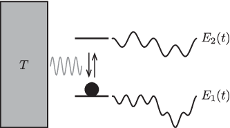
The first example is a work-to-work converter consisting of a particle that can hop between two discrete energy levels, cf. Fig. 1. Transitions are induced by a thermal bath, while the periodic modulation (period ) of the energy levels via two external work mechanisms allows the conversion of work extracted from the second source, driving the second energy level, and delivered to the first source, loading the first energy level. The time dependence of the energy in each level can be developed in terms of its Fourier components:
| (18) |
where the amplitudes and play the role of thermodynamic forces, refers to the Fourier mode, and and to cosine and sine, respectively. Following standard techniques from stochastic thermodynamics [58, 59, 60, 61, 62, 63], one can determine the explicit expression for the elements of the associated Onsager matrix [27] (cf. supplemental materials):
| (19) |
where and are the transition matrix and equilibrium probability distribution associated with the state of the particle in the absence of time-dependent driving, and . As a direct consequence of detailed balance, , one finds
| (20) |
Analogous relations are found for , with and . We conclude that the following symmetry relation holds:
| (21) |
which satisfies Eq. (17). Hence, the second set of power-efficiency-dissipation relations, Eq. (4,5) will be verified, see also [36] for a similar conclusion in a different model, and Fig. 2 for an illustration in case of a time-symmetric driving.


As another example of a system with broken time-reversal symmetry we consider a three-terminal thermoelectric device in a magnetic field, cf. Fig. 3. In this setup, three terminals are connected with each other via a central scattering region, inducing a particle flux and a heat flux . In the working regime, the heat flux is from high to low temperature, while the particle flux is from low to high chemical potential. We assume that both fluxes are in the direction of the second reservoir in Fig. 3. In this way heat is converted into chemical energy. A magnetic field, can be added to interact with the scattering region and break the time-reversal symmetry. An additional constraint which is often imposed is that the particle and heat flux through the third terminal vanish. The resulting Onsager matrix, associated with the heat and particle flux between reservoir and , is generally not symmetric, and the efficiency at maximum power can reach values up to [15], clearly violating the second set of power-efficiency-dissipation relations, Eqs. (4,5), cf. supplemental materials. Crucial to this analysis, however, is the constraint that the fluxes through the third terminal are zero, which makes it impossible to fully optimize the power output. Dropping the flux constraints will introduce thermodynamic sub-fluxes associated to the third terminal, and therefore and become matrices.
In the present context of linear thermodynamics, we set the reference values for temperature and chemical potential equal to those of the second reservoir, and . The fluxes can be decomposed into a net flux from the first to the second terminal and from the third to the second terminal, with associated thermodynamic forces and , where is the charge of one electron.
The behaviour of the central region is described by the scattering matrix, , which gives the fluxes of electrons with energy between the different terminals, when an external magnetic field, , is applied to the central region.
The resulting Onsager matrix is given by [64]:
| (22) |
with or , and the scattering matrix associated with the first and the third terminal only, and a function independent of the central scattering region, and in particular of the presence of a magnetic field (cf. supplemental materials). Hence, it is invariant under time-reversal symmetry and satisfies , implying . We conclude that Eqs. (4,5) will be valid when the optimization is carried out without constraints on the third terminal. In particular, the efficiency at maximum power will drop to a value below .
References
- [1] C. Van den Broeck, Physical Review Letters 95, 190602 (2005).
- [2] T. Schmiedl and U. Seifert, EPL (Europhysics Letters) 81, 20003 (2007).
- [3] T. Schmiedl and U. Seifert, EPL (Europhysics Letters) 83, 30005 (2008).
- [4] Z. Tu, Journal of Physics A: Mathematical and Theoretical 41, 312003 (2008).
- [5] B. Rutten, M. Esposito, and B. Cleuren, Physical Review B 80, 235122 (2009).
- [6] M. Esposito, K. Lindenberg, and C. Van den Broeck, Physical Review Letters 102, 130602 (2009).
- [7] M. Esposito, R. Kawai, K. Lindenberg, and C. Van den Broeck, Physical Review Letters 105, 150603 (2010a).
- [8] M. Esposito, R. Kawai, K. Lindenberg, and C. Van den Broeck, Physical Review E 81, 041106 (2010b).
- [9] G. Benenti, K. Saito, and G. Casati, Physical Review Letters 106, 230602 (2011).
- [10] J. Wang, J. He, and Z. Wu, Physical Review E 85, 031145 (2012).
- [11] Y. Izumida and K. Okuda, EPL (Europhysics Letters) 97, 10004 (2012).
- [12] N. Golubeva and A. Imparato, Physical Review Letters 109, 190602 (2012).
- [13] S. Sheng and Z. Tu, Journal of Physics A: Mathematical and Theoretical 46, 402001 (2013).
- [14] A. E. Allahverdyan, K. V. Hovhannisyan, A. V. Melkikh, and S. G. Gevorkian, Physical Review Letters 111, 050601 (2013).
- [15] K. Brandner, K. Saito, and U. Seifert, Physical Review Letters 110, 070603 (2013).
- [16] K. Brandner and U. Seifert, New Journal of Physics 15, 105003 (2013).
- [17] R. S. Whitney, Physical Review Letters 112, 130601 (2014).
- [18] Y. Wang, Phys. Rev. E 90, 062140 (2014).
- [19] Y. Izumida and K. Okuda, Physical Review Letters 112, 180603 (2014).
- [20] O. Entin-Wohlman, J.-H. Jiang, and Y. Imry, Physical Review E 89, 012123 (2014).
- [21] V. Holubec, Journal of Statistical Mechanics: Theory and Experiment 2014, P05022 (2014).
- [22] J. Stark, K. Brandner, K. Saito, and U. Seifert, Physical Review Letters 112, 140601 (2014).
- [23] J.-H. Jiang, Physical Review E 90, 042126 (2014).
- [24] M. Polettini, G. Verley, and M. Esposito, Physical Review Letters 114, 050601 (2015).
- [25] B. Cleuren, B. Rutten, and C. Van den Broeck, The European Physical Journal Special Topics 224, 879 (2015).
- [26] S. Sheng and Z. Tu, Physical Review E 91, 022136 (2015).
- [27] K. Proesmans and C. Van den Broeck, Physical Review Letters 115, 090601 (2015).
- [28] K. Brandner, K. Saito, and U. Seifert, Physical Review X 5, 031019 (2015).
- [29] K. Yamamoto and N. Hatano, Physical Review E 92, 042165 (2015).
- [30] V. Holubec and A. Ryabov, Physical Review E 92, 052125 (2015).
- [31] N. Shiraishi, K. Saito, and H. Tasaki, ArXiv e-prints (2016), 1605.00356 .
- [32] O. Raz, Y. Subaşı, and R. Pugatch, Physical Review Letters 116, 160601 (2016).
- [33] A. Ryabov and V. Holubec, arXiv preprint arXiv:1603.02623 (2016).
- [34] N. Shiraishi and K. Saito, arXiv preprint arXiv:1602.03645 (2016).
- [35] K. Proesmans, B. Cleuren, and C. Van den Broeck, Journal of Statistical Mechanics: Theory and Experiment 2016, 023202 (2016).
- [36] M. Bauer, K. Brandner, and U. Seifert, Physical Review E 93, 042112 (2016).
- [37] L. Cerino, A. Puglisi, and A. Vulpiani, Physical Review E 93, 042116 (2016).
- [38] Eq. (49) from [36] is identical to the second part of our Eq. (5) provided one identifies the ’idle heat flux’ with our minimal dissipation .
- [39] Onsager anti-symmetry is defined by for all .
- [40] I. Prigogine, Introduction to thermodynamics of irreversible processes (New York: Interscience, 1967, 3rd ed., 1967).
- [41] S. R. De Groot and P. Mazur, Non-equilibrium thermodynamics (Courier Corporation, 2013).
- [42] The temperature of the power producing device is the natural choice for the multiplicative factor . We however stress that the results Eqs. (1-5) are valid, irrespective of the choice of this temperature.
- [43] H. B. G. Casimir, Reviews of Modern Physics 17, 343 (1945).
- [44] L. Onsager, Physical Review 37, 405 (1931a).
- [45] L. Onsager, Physical Review 38, 2265 (1931b).
- [46] Y. Izumida and K. Okuda, Physical Review E 80, 021121 (2009).
- [47] Y. Izumida and K. Okuda, The European Physical Journal B 77, 499 (2010).
- [48] O. Raz, Y. Subasi, and C. Jarzynski, arXiv preprint arXiv:1509.06323 (2015).
- [49] G. Falasco and M. Baiesi, EPL (Europhysics Letters) 113, 20005 (2016).
- [50] M. Büttiker, IBM Journal of Research and Development 32, 317 (1988).
- [51] D. Sánchez and L. Serra, Physical Review B 84, 201307 (2011).
- [52] O. Entin-Wohlman and A. Aharony, Physical Review B 85, 085401 (2012).
- [53] V. Balachandran, G. Benenti, and G. Casati, Physical Review B 87, 165419 (2013).
- [54] H. Thierschmann, R. Sánchez, B. Sothmann, F. Arnold, C. Heyn, W. Hansen, H. Buhmann, and L. W. Molenkamp, Nat Nano 10, 854 (2015).
- [55] R. Sánchez, B. Sothmann, and A. N. Jordan, Physical Review Letters 114, 146801 (2015a).
- [56] R. Sánchez, B. Sothmann, and A. N. Jordan, New Journal of Physics 17, 075006 (2015b).
- [57] P. P. Hofer and B. Sothmann, Physical Review B 91, 195406 (2015).
- [58] R. Harris and G. Schütz, Journal of Statistical Mechanics: Theory and Experiment 2007, P07020 (2007).
- [59] K. Sekimoto, Stochastic energetics, Vol. 799 (Springer, 2010).
- [60] U. Seifert, Reports on Progress in Physics 75, 126001 (2012).
- [61] R. Spinney and I. Ford, in Nonequilibrium Statistical Physics of Small Systems: Fluctuation Relations and Beyond, edited by H. G. Schuster, R. Klages, W. Just, and C. Jarzynski (John Wiley & Sons, 2013).
- [62] C. Van den Broeck and M. Esposito, Physica A: Statistical Mechanics and its Applications 418, 6 (2014).
- [63] T. Tomé and M. J. de Oliveira, Physical Review E 91, 042140 (2015).
- [64] U. Sivan and Y. Imry, Physical Review B 33, 551 (1986).