Preparing topologically ordered states
by Hamiltonian interpolation
Abstract
We study the preparation of topologically ordered states by interpolating between an initial Hamiltonian with a unique product ground state and a Hamiltonian with a topologically degenerate ground state space. By simulating the dynamics for small systems, we numerically observe a certain stability of the prepared state as a function of the initial Hamiltonian. For small systems or long interpolation times, we argue that the resulting state can be identified by computing suitable effective Hamiltonians. For effective anyon models, this analysis singles out the relevant physical processes and extends the study of the splitting of the topological degeneracy by Bonderson [18]. We illustrate our findings using Kitaev’s Majorana chain, effective anyon chains, the toric code and Levin-Wen string-net models.
1 Introduction
Topologically ordered phases of matter have attracted significant interest in the field of quantum information, following the seminal work of Kitaev [36]. From the viewpoint of quantum computing, one of their most attractive features is their ground space degeneracy: it provides a natural quantum error-correcting code for encoding and manipulating information. Remarkably, the ground space degeneracy is approximately preserved in the presence of weak static Hamiltonian perturbations [8, 7, 45]. This feature suppresses the uncontrolled accumulation of relative phases between code states, and thus helps to overcome decoherence. This is a necessary requirement for the realization of many-body quantum memories [25].
To use topologically ordered systems as quantum memories and for fault-tolerant quantum computation, concrete procedures for the preparation of specific ground states are required. Such mechanisms depend on the model Hamiltonian which is being realized as well as on the particular experimental realization. Early work [25] discussed the use of explicit unitary encoding circuits for the toric code. This consideration is natural for systems where we have full access to unitary gates over the underlying degrees of freedom. We may call this the bottom-up approach to quantum computing: here one proceeds by building and characterizing individual components before assembling them into larger structures. An example are arrays of superconducting qubits [14, 23, 24]. Other proposed procedures for state preparation in this approach involve engineered dissipation [26, 4] or measurement-based preparation [42]. However, achieving the control requirements for experimentally performing such procedures is quite challenging. They require either a) independently applying complex sequences of gates on each of the elementary constituents b) precisely engineering a dissipative evolution, or c) performing an extensive set of local measurements and associated non-local classical data processing to determine and execute a suitable unitary correction operation. Imperfections in the implementation of such protocols pose a severe problem, especially in cases where the preparation time is extensive [9, 41].
In fact, these procedures achieve more than is strictly necessary for quantum computation: any ground state can be prepared in this fashion. That is, they constitute encoders, realizing an isometry from a number of unencoded logical qubits to the ground space of the target Hamiltonian. We may ask if the task of preparing topologically ordered state becomes easier if the goal is to prepare specific states instead of encoding arbitrary states. In particular, we may ask this question in the top-down approach to quantum computing, where the quantum information is encoded in the ground space of a given condensed matter Hamiltonian. An example are Majorana wires [46, 47] or fractional quantum Hall substrates [59]. Indeed, a fairly standard approach to preparing ground states of a Hamiltonian is to cool the system by weakly coupling it with a thermal bath at a temperature significantly lower than the Hamiltonian gap. Under appropriate ergodicity conditions, this leads to convergence to a state mainly supported on the ground space. Unfortunately, when using natural equilibration processes, convergence may be slow, and the resulting prepared state is generally a (logical) mixed state unsuitable for computation.
A natural alternative method for preparing ground states of a given Hamiltonian is adiabatic evolution: here one initializes the system in an easy-to-prepare state (e.g., a product state), which is the unique ground state of a certain initial Hamiltonian (e.g., describing a uniform field). Subsequently, the Hamiltonian of the system is gradually changed (by tuning external control parameters in a time-dependent fashion) until the target Hamiltonian is reached. If this time-dependent change of the Hamiltonian is “slow enough”, i.e., satisfies a certain adiabaticity condition (see Section 2), the state of the system will closely follow the trajectory of instantaneous ground states. The resulting state then is guaranteed to be mainly supported on the ground space of the target Hamiltonian, as desired.
Adiabatic preparation has some distinct advantages compared to e.g., encoding using a unitary circuit. For example, in contrast to the latter, adiabatic evolution guarantees that the final state is indeed a ground state of the actual Hamiltonian describing the system, independently of potential imperfections in the realization of the ideal Hamiltonians. In contrast, a unitary encoding circuit is designed to encode into the ground space of an ideal model Hamiltonian, and will therefore generally not prepare exact ground states of the actual physical system (which only approximate the model Hamiltonian). Such an encoding into the ideal ground space may lead to a negligible quantum memory time in the presence of an unknown perturbation [51]; this is because ideal and non-ideal (perturbed) ground states may differ significantly (this phenomenon is referred to as Anderson’s orthogonality catastrophe [3]). Adiabatic evolution, on the other hand, elegantly sidesteps these issues.
The fact that adiabatic evolution can follow the actual ground state of a system Hamiltonian makes it a natural candidate for achieving the task of topological code state preparation. An additional attractive feature is that its experimental requirements are rather modest: while some time-dependent control is required, this can be local, and additionally translation-invariant. Namely, the number of external control parameters required does not scale with the system size or code distance.
Summary and outlook
Motivated by these observations, we consider the general problem of preparing topologically ordered states by what we refer to as Hamiltonian interpolation. We will use this terminology instead of “adiabatic evolution” since in some cases, it makes sense to consider scenarios where adiabaticity guarantees cannot be given. For concreteness, we consider a time-dependent Hamiltonian which monotonically sweeps over the path
| (1) |
i.e., we assume that the interpolation is linear in time and takes overall time11 1 We remark that in some cases, using a non-linear monotone ‘schedule’ with , and smooth derivatives may be advantageous (see Discussion in Section 2). However, for most of our considerations, the simple linear interpolation (1) is sufficient. . Guided by experimental considerations, we focus on the translation-invariant case: here the Hamiltonians are translation-invariant throughout the evolution. More precisely, we consider the process of interpolating between a Hamiltonian with unique ground state and a Hamiltonian with topologically degenerate ground space (which is separated from the remainder of the spectrum by a constant gap): the state of the system at time satisfies the equation of motion
| (2) |
Generally, we consider families of Hamiltonians (or models) parametrized by a system size ; throughout, we will assume that is the number of single particles, e.g., the number of qubits (or sites) in a lattice with Hilbert space . The dimension of the ground space of will be assumed to be independent of the system size.
Our goal is to characterize the set of states which are preparable by such Hamiltonian interpolations starting from various product states, i.e., by choosing different initial Hamiltonians . To each choice of product state we associate a normalized initial trivial Hamiltonian which fully specifies the interpolating path of Eq. (1), with being the single particle projector onto the state at site .
In the limit , one may think of this procedure as associating an encoded (logical) state to any single-particle state . However, some caveats are in order: first, the global phase of the state cannot be defined in a consistent manner in the limit , and is therefore not fixed. Second, the final state in the evolution (2) does not need to be supported entirely on the ground space of because of non-adiaticity errors, i.e., it is not a logical (encoded) state itself. To obtain a logical state, we should think of as the final state projected onto the ground space of . Up to these caveats, our goal is essentially to characterize the image of the association , as well as its continuity properties. We will also define an analogous map associated to fixed evolution time and study it numerically by simulating the corresponding Schrödinger equation (2) on a classical computer.
While there is a priori no obvious relationship between the final states , resulting from different initial (product) states , we numerically find that the image of is concentrated around a particular discrete family of encoded states. In particular, we observe for small system sizes that the preparation enjoys a certain stability property: variations in the initial Hamiltonian do not significantly affect the final state. We support this through analytic arguments, computing effective Hamiltonians associated to perturbations around which address the large limit. This also allows us to provide a partial prediction of which states may be obtained through such a preparation process. We find that under certain general conditions, belongs to a certain finite family of preferred states which depend on the final Hamiltonian . As we will argue, there is a natural relation between the corresponding states for different system sizes: they encode the same logical state if corresponding logical operators are chosen (amounting to a choice of basis of the ground space).
Characterizing the set of states preparable using this kind of Hamiltonian interpolation is important for quantum computation because certain encoded states (referred to as “magic states”) can be used as a resource for universal computation [11]. Our work provides insight into this question for ‘small’ systems, which we deem experimentally relevant. Indeed, there is a promising degree of robustness for the Hamiltonian interpolation to prepare certain (stabilizer) states. However, a similar preparation of magic states seems to require imposing additional symmetries which will in general not be robust. We exemplify our considerations using various concrete models, including Kitaev’s Majorana chain [35] (for which we can provide an exact solution), effective anyon chains (related to the so-called golden chain [28] and the description used by Bonderson [18]), as well as the toric code [36] and Levin-Wen string-net models [44] (for which we simulate the time-evolution for small systems, for both the doubled semion and the doubled Fibonacci model).
Prior work
The problem of preparing topologically ordered states by adiabatic interpolation has been considered prior to our work by Hamma and Lidar [31]. Indeed, their contribution is one of the main motivations for our study. They study an adiabatic evolution where a Hamiltonian having a trivial product ground state is interpolated into a toric code Hamiltonian having a four-fold degenerate ground state space. They found that while the gap for such an evolution must forcibly close, this may happen through second order phase transitions. Correspondingly, the closing of the gap is only polynomial in the system size. This allows an efficient polynomial-time Hamiltonian interpolation to succeed at accurately preparing certain ground states. We revisit this case in Section 2.1 and give further examples of this phenomenon. The authors of [32] also observed the stability of the encoded states with respect to perturbations in the preparation process.
Bonderson [18] considered the problem of characterizing the lowest order degeneracy splitting in topologically ordered models. Degeneracy lifting can be associated to tunneling of anyonic charges, part of which may be predicted by the universal algebraic structure of the anyon model. Our conclusions associated to Sections 5 and 6 can be seen as supporting this perspective.
Beyond small systems
In general, the case of larger systems (i.e., the thermodynamic limit) requires a detailed understanding of the quantum phase transitions [55] occurring when interpolating between and . Taking the thermodynamic limit while making scale as a polynomial of the system size raises a number of subtle points. A major technical difficulty is that existing adiabatic theorems do not apply, since at the phase transition gaps associated to either of the relevant phases close. This is alleviated by scaling the interpolation time with the system size and splitting the adiabatic evolution into two regimes, the second of which can be treated using degenerate adiabatic perturbation theory [52, 53, 54]. However, such a methodology still does not yield complete information about the dynamical effects of crossing a phase boundary.
More generally, it is natural to conjecture that interpolation between different phases yields only a discrete number of distinct states corresponding to a discrete set of continuous phase transitions in the thermodynamic limit. Such a conjecture links the problem of Hamiltonian interpolation to that of classifying phase transitions between topological phases. It can be motivated by the fact that only a discrete set of possible condensate-induced continuous phase transitions is predicted to exist in the thermodynamic limit [19, 20].
2 Adiabaticity and ground states
The first basic question arising in this context is whether the evolution (2) yields a state close to the ground space of . The adiabatic theorem in its multiple forms (see e.g., [58]) provides sufficient conditions for this to hold: These theorems guarantee that given a Hamiltonian path satisfying certain smoothness and gap assumptions, initial eigenstates evolve into approximate instantaneous eigenstates under an evolution of the form (2). The latter assumptions are usually of the following kind:
- (i)
Uniform gap: There is a uniform lower bound on the spectral gap of for all . The relevant spectral gap is the energy difference between the ground space of the instantaneous Hamiltonian and the rest of its spectrum. Here and below, we denote by the spectral projection onto the ground space 22 2 More generally, may be the sum of the spectral projections of with eigenvalues in a given interval, which is separated by a gap from the rest of the spectrum. of .
- (ii)
Smoothness: There are constants such that the first derivatives of are uniformly bounded in operator norm, i.e., for all , we have
(3)
The simplest version of such a theorem is:
Theorem 2.1.
This version is sufficient to support our analytical conclusions qualitatively. For a quantitative analysis of non-adiabaticity errors, we perform numerical simulations. Improved versions of the adiabatic theorem (see [30, 43]) provide tighter analytical error estimates for general interpolation schedules at the cost of involving higher order derivatives of the Hamiltonian path (see Eq.‘(3)), but do not change our main conclusions.
Several facts prevent us from directly applying such an adiabatic theorem to our evolution (1) under consideration.
Topological ground space degeneracy.
Most notably, the gap assumption (i) is not satisfied if we study ground spaces: we generally consider the case where has a unique ground state, whereas the final Hamiltonian is topologically ordered and has a degenerate ground space (in fact, this degeneracy is exact and independent of the system size for the models we consider). This means that if is the projection onto the ground space of , there is no uniform lower bound on the gap .
We will address this issue by restricting our attention to times , where is chosen such that has a non-vanishing gap but still is “inside the topological phase”. We will illustrate in specific examples how can indeed be recovered by taking the limit .
We emphasize that the expression “inside the phase” is physically not well-defined at this point since we are considering a Hamiltonian of a fixed size. Computationally, we take it to mean that the Hamiltonian can be analyzed by a convergent perturbation theory expansion starting from the unperturbed Hamiltonian . The resulting lifting of the ground space degeneracy of will be discussed in more detail in Section 3.
Dependence on the system size.
A second potential obstacle for the use of the adiabatic theorem is the dependence on the system size (where e.g., is the number of qubits). This dependence enters in the operator norms (3), which are extensive in – this would lead to polynomial dependence of on even if e.g., the gap were constant (uniformly bounded).
More importantly, the system size enters in the gap : in the topological phase, the gap (i.e., the splitting of the topological degeneracy of ) is exponentially small in for constant-strength local perturbations to , as shown for the models considered here by Bravyi, Hastings and Michalakis [8]. Thus a naïve application of the adiabatic theorem only yields a guarantee on the ground space overlap of the final state if the evolution time is exponentially large in . This is clearly undesirable for large systems; one may try to prepare systems faster (i.e., more efficiently) but would need alternate arguments to ensure that the final state indeed belongs to the ground space of .
For these reasons, we restrict our attention to the following two special cases of the Hamiltonian interpolation (1):
- •
Symmetry-protected preparation: if there is a set of observables commuting with both and , these will represent conserved quantities throughout the Hamiltonian interpolation. If the initial state is an eigenstate of such observables, one may restrict the Hilbert space to the relevant eigenvalue, possibly resolving the topological degeneracy and guaranteeing a uniform gap. This observation was first used in [31] in the context of the toric code: for this model, such a restriction allows mapping the problem to a transverse field Ising model, where the gap closes polynomialy with the system size. We identify important cases satisfying this condition. While this provides the most robust preparation scheme, the resulting encoded states are somewhat restricted (see Section 2.1).
- •
Small systems: For systems of relatively small (constant) size , the adiabatic theorem can be applied as all involved quantities are essentially constant. In other words, although ‘long’ interpolation times are needed to reach ground states of (indeed, these may depend exponentially on ), these may still be reasonable experimentally. The consideration of small system is motivated by current experimental efforts to realize surface codes [34]: they are usually restricted to a small number of qubits, and this is the scenario we are considering here (see Section 2.2).
Obtaining a detailed understanding of the general large limiting behaviour (i.e., the thermodynamic limit) of the interpolation process (1) is beyond the scope of this work.
2.1 Symmetry-protected preparation
Under particular circumstances, the existence of conserved quantities permits applying the adiabatic theorem while evading the technical obstacle posed by a vanishing gap in the context of topological order. Such a case was considered by Hamma and Lidar [31], who showed that certain ground states of the toric code can be prepared efficiently. We can formalize sufficient conditions in the following general way (which then is applicable to a variety of models, as we discuss below).
Observation 2.2.
Consider the interpolation process (1) in a Hilbert space . Let be the projection onto the ground space of . Suppose that is a projection such that
- (i)
is a conserved quantity: .
- (ii)
The initial state is the ground state of , i.e., and satisfies .
- (iii)
The final ground space has support on
- (iv)
The restriction of to has gap which is bounded by a constant uniformly in , i.e., for all .
Then , and the adiabatic theorem can be applied with lower bound on the gap, yielding .
The proof of this statement is a straightforward application of the adiabatic theorem (Theorem 2.1) to the Hamiltonians and in the restricted subspace . In the following sections, we will apply Observation 2.2 to various systems. It not only guarantees that the ground space is reached, but also gives us information about the specific state prepared in a degenerate ground space.
As an example of the situation discussed in Observation 2.2, we discuss the case of fermionic parity conservation in Section 4. This symmetry is naturally present in fermionic systems. We expect our arguments to extend to more general topologically ordered Hamiltonians with additional symmetries. It is well-known that imposing global symmetries on top of topological Hamiltonians provides interesting classes of systems. Such symmetries can exchange anyonic excitations, and their classification as well as the construction of associated defect lines in topological Hamiltonians is a topic of ongoing research [21, 38, 10]. The latter problem is intimately related to the realization (see e.g., [16, 17]) of transversal logical gates, which leads to similar classification problems [13, 5, 62, 61]. Thus we expect that there is a close connection between adiabatically preparable states and transversally implementable logical gates. Indeed, a starting point for establishing such a connection could be the consideration of interpolation processes respecting symmetries realized by transversal logical gates.
For later reference, we also briefly discuss a situation involving conserved quantities which – in contrast to Observation 2.2 – project onto excited states of the final Hamiltonian. In this case, starting with certain eigenstates of the corresponding symmetry operator , the ground space cannot be reached:
Observation 2.3.
The proof of this observation is trivial since is a conserved quantity of the Schrödinger evolution. Physically, the assumptions imply the occurrence of a level-crossing where the energy gap exactly vanishes and eigenvalue of restricted to the ground space changes. We will encounter this scenario in the case of the toric code on a honeycomb lattice, see Section 7.3.
2.2 Small-system case
In a more general scenario, there may not be a conserved quantity as in Observation 2.2. Even assuming that the ground space is reached by the interpolation process (1), it is a priori unclear which of the ground states is prepared. Here we address this question.
As remarked earlier, we focus on systems of a constant size , and assume that the preparation time is large compared to . Generically, the Hamiltonians are then non-degenerate (except at the endpoint, , where approaches ). Without fine tuning, we may expect that there are no exact level crossings in the spectrum of along the path (say for some times , ). For sufficiently large overall evolution times , we may apply the adiabatic theorem to conclude that the state of the system follows the (unique) instantaneous ground state (up to a constant error). Since our focus is on small systems, we will henceforth assume that this is indeed the case, and summarily refer to this as the adiabaticity assumption. Again, we emphasize that this is a priori only reasonable for small systems.
Under the adiabaticity assumption, we can conclude that the prepared state roughly coincides with the state obtained by computing the (unique) ground state of , and taking the limit . In what follows, we adopt this computational prescription for identifying prepared states. Indeed, this approach yields states that match our numerical simulation, and provides the correct answer for certain exactly solvable cases. Furthermore, the computation of the states (in the limit ) also clarifies the physical mechanisms responsible for the observed stability property of preparation: we can relate the prepared states to certain linear combination of string-operators (Wilson-loops), whose coefficients depend on the geometry (length) of these loops, as well as the amplitudes of certain local particle creation/annihilation and tunneling processes.
Since for is close to the topologically ordered Hamiltonian , it is natural to use ground states (or logical operators) of the latter as a reference to express the instantaneous states . Indeed, the problem essentially reduces to a system described by , with an additional perturbation given by a scalar multiple of . Such a local perturbation generically splits the topological degeneracy of the ground space. The basic mechanism responsible for this splitting for topologically ordered systems has been investigated by Bonderson [18], who quantified the degeneracy splitting in terms of local anyon-processes. We seek to identify low-energy ground states: this amounts to considering the effective low-energy dynamics (see Section 3). This will provide valuable information concerning the set .
3 Effective Hamiltonians
As discussed in Section 2.2, for small systems (and sufficiently large times ), the state in the interpolation process (1) should coincide with the ground state of the instantaneous Hamiltonian . For , the latter is a perturbed version of the Hamiltonian , where the perturbation is a scalar multiple of . That is, up to rescaling by an overall constant, we are concerned with a Hamiltonian of the form
| (5) |
where is the target Hamitonian and is the perturbation. To compute the ground state of a Hamiltonian of the form (5), we use effective Hamiltonians. These provide a description of the system in terms of effective low-energy degrees of freedom.
3.1 Low-energy degrees of freedom
Let us denote by the projection onto the degenerate ground space of . Since is assumed to have a constant gap, a perturbation of the form (5) effectively preserves the low-energy subspace for small , and generates a dynamics on this subspace according to an effective Hamiltonian . We will discuss natural definitions of this effective Hamiltonian in Section 3.3. For the purpose of this section, it suffices to mention that it is entirely supported on the ground space of , i.e., . As such, it has spectral decomposition
| (6) |
where , and where are commuting projections onto subspaces of the ground space of . (Generally, we expect to be non-degenerate such that .) In particular, the effective Hamiltonian (6) gives rise to an orthogonal decomposition of the ground space by projections . States in are distinguished by having minimal energy. We can take the limiting projections as the perturbation strength goes to , setting
In particular, the effective Hamiltonian has ground space in the limit . Studying , and, in particular, the space appears to be of independent interest, as it determines how perturbations affect the topologically ordered ground space beyond spectral considerations as in [18].
3.2 Hamiltonian interpolation and effective Hamiltonians
The connection to the interpolation process (1) is then given by the following conjecture. It is motivated by the discussion in Section 2.2 and deals with the case where there are no conserved quantities (unlike, e.g., in the case of the Majorana chain, as discussed in Section 4).
Conjecture 1.
Under suitable adiabaticity assumptions (see Section 2.2) the projection of the final state onto the ground space of belongs to (up to negligible errors33 3 By negligible, we mean that the errors can be made to approach zero as is increased.), i.e., it is a ground state of the effective Hamiltonian in the limit .
In addition to the arguments in Section 2.2, we provide evidence for this conjecture by explicit examples, where we illustrate how can be computed analytically. We also verify that Conjecture 1 correctly determines the final states by numerically studying the evolution (1).
We remark that the statement of Conjecture 1 severly constrains the states that can be prepared by Hamiltonian interpolation in the large limit: we will argue that the space has a certain robustness with respect to the choice of the initial Hamiltonian . In fact, the space is typically -dimensional and spanned by a single vector . Furthermore, this vector typically belongs to a finite family of states defined solely by . In particular, under Conjecture 1, the dependence of the final state on the Hamiltonian is very limited: the choice of only determines which of the states in is prepared. We numerically verify that the resulting target states indeed belong to the finite family of states obtained analytically.
3.3 Perturbative effective Hamiltonians
As discussed in Section 3.2, we obtain distinguished final ground states by computation of suitable effective Hamiltonians , approximating the action of on the ground space of . In many cases of interest, computing this effective Hamiltonian (whose definition for the Schrieffer-Wolff-case we present in Appendix A.1) exactly is infeasible (The effective Hamiltonian for the Majorana chain (see Section 4) is an exception.).
Instead, we seek a perturbative expansion
| (7) |
in terms of powers of the perturbation strength . This is particularly natural as we are interested in the limit anyway (see Conjecture 1). Furthermore, it turns out that such perturbative expansions provide insight into the physical mechanisms underlying the ‘selection’ of particular ground states.
We remark that there are several different methods for obtaining low-energy effective Hamiltonians. The Schrieffer-Wolff method [57, 6] provides a unitary such that preserves and can be regarded as an effective Hamiltonian. One systematically obtains a series expansion
for the anti-Hermitian generator of ; this then naturally gives rise to an order-by-order expansion
| (8) |
of the effective Hamiltonian, where is the projection onto the ground space of (explicit expressions are given in Appendix A.2).
Using the Schrieffer-Wolff method has several distinct advantages, including the fact that
- (i)
the resulting effective Hamiltonian , as well as the terms are Hermitian, and hence have a clear physical interpretation. This is not the case e.g., for the Bloch expansion [15].
- (ii)
We point out that the series resulting by taking the limit in (8) has the usual convergence issues encountered in many-body physics: convergence is guaranteed only if , where is the gap of . For a many-body system with extensive Hilbert space (e.g., spins), the norm is extensive while the gap is constant, leading to convergence only in a regime where . In this respect, the Schrieffer-Wolff method does not provide direct advantages compared to other methods. As we are considering the limit , this is not an issue (also, for small systems as those considered in our numerics, we do not have such issues either).
We point out, however, that the results obtained by Bravyi et al. [6] suggest that considering partial sums of the form (8) is meaningful even in cases in which the usual convergence guarantees are not given: indeed, [6, Theorem 3] shows that the ground state energies of and are approximately equal for suitable choices of and . Another key feature of the Schrieffer-Wolff method is the fact that the effective Hamiltonians are essentially local (for low orders ) when the method is applied to certain many-body systems, see [6]. We will not need the corresponding results here, however.
Unfortunately, computing the Schrieffer-Wolff Hamiltonian generally involves a large amount of combinatorics (see [6] for a diagrammatic formalism for this purpose). In this respect, other methods may appear to be somewhat more accessible. Let us mention in particular the method involving the Dyson equation (and the so-called ‘self-energy’ operator), which was used e.g., in [37, Section 5.1] to compute -th order effective Hamiltonians. This leads to remarkably simple expressions of the form
| (9) |
for the -th order term effective Hamiltonian, where is the resolvent operator
| (10) |
evaluated at the ground state energy of . In general, though, the expression (9) only coincides with the Schrieffer-Wolff-method (that is, (8)) up to the lowest non-trivial order.
3.4 Perturbative effective Hamiltonians for topological order
Here we identify simple conditions under which the Schrieffer-Wolff Hamiltonian of lowest non-trivial order has the simple structure (9). We will see that these conditions are satisfied for the systems we are interested in. In other words, for our purposes, the self-energy methods and the Schrieffer-Wolff method are equivalent. While establishing this statement (see Theorem 3.2 below) requires some work, this result vastly simplifies the subsequent analysis of concrete systems.
The condition we need is closely related to quantum error correction [40]. In fact, this condition has been identified as one of the requirements for topological quantum order (TQO-1) in Ref. [8]. To motivate it, consider the case where is an error-correcting code of distance . Then all operators acting on less than particles44 4 By particle we mean a physical constituent qubit or qudit degree of freedom. have trivial action on the code space, i.e., for such , the operator is proportional to (which we will write as ). In particular, this means that if is a Hermitian linear combination of single-particle operators, then for all . The condition we need is a refinement of this error-correction criterion that incorporates energies (using the resolvent):
Definition 3.1.
We say that the pair satisfies the topological order condition with parameter if is the smallest interger such that for all , we have
| (11) |
for all . Here is the ground space projection of , is the projection onto the orthogonal complement, and is the resolvent (10) (supported on ).
We remark that this definition is easily verified in the systems we consider: if excitations in the system are local, the resolvent operators and projection in a product of the form (11) can be replaced by local operators, and condition (11) essentially reduces to a standard error correction condition for operators with local support.
Assuming this definition, we then have the following result:
Theorem 3.2.
Suppose that satisfies the topological order condition with parameter . Then the -th order Schrieffer-Wolff effective Hamiltonian satisfies
| (12) |
i.e., the effective Hamiltonian is trivial for these orders, and
| (13) |
We give the proof of this statement in Appendix A.
4 The Majorana chain
In this section, we apply our general results to Kitaev’s Majorana chain. We describe the model in Section 4.1. In Section 4.2, we argue that the interpolation process (2) is an instance of symmetry-protected preparation; this allows us to identify the resulting final state. We also observe that the effective Hamiltonian is essentially given by a ‘string’-operator , which happens to be the fermionic parity operator in this case. That is, up to a global energy shift, we have
| (14) |
for a certain constant depending on the choice of perturbation.
4.1 The model
Here we consider the case where is Kitaev’s Majorana chain [35], a system of spinless electrons confined to a line of sites. In terms of Majorana operators satisfying the anticommutation relations
as well as , , the Hamiltonian has the form
| (15) |
Without loss of generality, we have chosen the normalization such that elementary excitations have unit energy. The Hamiltonian has a two-fold degenerate ground space. The Majorana operators and correspond to a complex boundary mode, and combine to form a Dirac fermion
| (16) |
which commutes with the Hamiltonian. The operator hence provides a natural occupation number basis for the ground space defined (up to arbitrary phases) by
| (17) |
As a side remark, note that the states and cannot be used directly to encode a qubit. This is because they have even and odd fermionic parity, respectively, and thus belong to different superselection sectors. In other words, coherent superposition between different parity sectors are nonphysical. This issue can be circumvented by using another fermion or a second chain, see [12]. Since the conclusions of the following discussion will be unchanged, we will neglect this detail for simplicity.
We remark that the Hamiltonian of Eq. (15) belongs to a one-parameter family of extensively studied and well-understood quantum spin Hamiltonians. Indeed, the Jordan-Wigner transform of the Hamiltonian (with an arbitrary parameter)
| (18) |
is the transverse field Ising model
| (19) |
where and are the spin Pauli matrices acting on qubit , . This transformation allows analytically calculating the complete spectrum of the translation invariant chain for both periodic and open boundary conditions [50].
The Hamiltonian has a quantum phase transition at , for which the lowest energy modes in the periodic chain have an energy scaling as . The open boundary case has been popularized by Kitaev as the Majorana chain and has a unique low energy mode (see Eq. (16)) which has zero energy for and for finite , becomes a dressed mode with exponentially small energy (in ) and which is exponentially localized at the boundaries.
4.2 State preparation by interpolation
The second term in (18) may be taken to be the initial Hamiltonian for the interpolation process. More generally, to prepare ground states of , we may assume that our initial Hamiltonian is a quadratic Hamiltonian with a unique ground state. That is, is of the form
| (20) |
where is a real antisymmetric matrix. We will assume that it is bounded and local (with range ) in the sense that
| (21) |
where denotes the operator norm. As shown in [12, Theorem 1], the Hamiltonian has two lowest energy states with exponentially small energy difference, and this lowest-energy space remains separated from the rest of the spectrum by a constant gap for a fixed (constant) perturbation strength . Estimates on the gap along the complete path are, to the best of our knowledge, not known in this more general situation.
Let us assume that is the unique ground state of and consider the linear interpolation (2). The corresponding process is an instance of the symmetry-protected preparation, i.e., Observation 2.2 applies in this case. Indeed, the fermionic parity operator
| (22) |
commutes with both and . Therefore, the initial ground state lies either in the even-parity sector, i.e., , or in the odd-parity sector (). (Even parity is usually assumed by convention, since the fermionic normal modes used to describe the system are chosen to have positive energy.) In any case, the eigenvalue of the initial ground state with respect to will persist throughout the full interpolation. This fixes the final state:
Lemma 4.1.
In particular, if is given by the second term in (18), we can apply the results of [50]: the gap at the phase transition is associated with the lowest energy mode (which is not protected by symmetry) and is given by . In other words, it is linearly decreasing in the system size . Therefore, the total evolution time only needs to grow polynomially in the system size for Hamiltonian interpolation to accurately follow the ground state space at the phase transition. We conclude that translation-invariant Hamiltonian interpolation allows preparing the state in a time polynomial in the system size and the desired approximation accuracy.
To achieve efficient preparation through Hamiltonian interpolation, one issue that must be taken into account is the effect of disorder (possibly in the form of a random site-dependent chemical potential). In the case where the system is already in the topologically ordered phase, a small amount of Hamiltonian disorder can enhance the zero temperature memory time of the Majorana chain Hamiltonian [12]. This 1D Anderson localization effect [2], while boosting memory times, was also found to hinder the convergence to the topological ground space through Hamiltonian interpolation. Indeed, in [22] it was found that the residual energy density averaged over disorder realizations decreases only polylogarithmically with the Hamiltonian interpolation time. Such a slow convergence of the energy density indicates that in the presence of disorder, the time required to accurately reach the ground space scales exponentially with the system size . For this reason, translation-invariance (i.e., no disorder) is required for an efficient preparation, and this may be challenging in practice.
We emphasize that according to Lemma 4.1, the prepared state is largely independent of the choice of the initial Hamiltonian (amounting to a different choice of ): we do not obtain a continuum of final states. As we will see below, this stability property appears in a similar form in other models. The parity operator (22), which should be thought of as a string-operator connecting the two ends of the wire, plays a particular role – it is essentially the effective Hamiltonian which determines the prepared ground state.
Indeed, the Schrieffer-Wolff-effective Hamiltonian can be computed exactly in this case, yielding
| (23) |
where is the ground state energy of , and is the gap. Expression (23) can be computed based on the variational expression (111) for the Schrieffer-Wolff transformation, using the fact that the ground space is two-dimensional and spanned by two states belonging to the even- and odd-parity sector, respectively. Note that the form (23) can also be deduced (without the exact constants) from the easily verified fact (see e.g., Eq. (109)) that the Schrieffer-Wolff unitary commutes with the fermionic parity operator , and thus the same is true for . This expression illustrates that Conjecture 1 does not directly apply in the context of preserved quantities, as explained in Section 3.2: rather, it is necessary to know the parity of the initial state to identify the resulting final state in the interpolation process.
5 General anyon chains
In this section, we generalize the considerations related to the Majorana chain to more general anyonic systems. Specifically, we consider a -dimensional lattice of anyons with periodic boundary conditions. This choice retains many features from the Majorana chain such as locally conserved charges and topological degeneracy yet further elucidates some of the general properties involved in the perturbative lifting of the topological degeneracy.
In Section 5.1, we review the description of effective models for topologically ordered systems. A key feature of these models is the existence of a family of string-operators indexed by particle labels. Physically, the operators correspond to the process of creating a particle-antiparticle pair , tunneling along the -dimensional (periodic) lattice, and subsequent fusion of the pair to the vacuum (see Section 5.1.6). These operators play a fundamental role in distinguishing different ground states.
In Section 5.2, we derive our main result concerning these models. We consider local translation-invariant perturbations to the Hamiltonian of such a model, and show that the effective Hamiltonian is a linear combination of string-operators, i.e.,
| (24) |
up to an irrelevant global energy shift. The coefficients are determined by the perturbation. They can be expressed in terms of a certain sum of diagrams, as we explain below. While not essential for our argument, translation-invariance allows us to simplify the parameter dependence when expressing the coefficients and may also be important for avoiding the proliferation of small gaps.
We emphasize that the effective Hamiltonian has the form (24) independently of the choice of perturbation. The operators are mutually commuting, and thus have a distinguished simultaneous eigenbasis (we give explicit expressions for the latter in Section 5.1.6). The effective Hamiltonian (24) is therefore diagonal in a fixed basis irrespective of the considered perturbation. Together with the general reasoning for Conjecture 1, this suggests that Hamiltonian interpolation can only prepare a discrete family of different ground states in these anyonic systems.
In Section 6, we consider two-dimensional topologically ordered systems and find effective Hamiltonians analogous to (24). We will also show numerically that Hamiltonian interpolation indeed prepares corresponding ground states.
5.1 Background on anyon chains
The models we consider here describe effective degrees of freedom of a topologically ordered system. Concretely, we consider one-dimensional chains with periodic boundary conditions, where anyonic excitations may be created/destroyed on sites, and may hop between neighboring sites. Topologically (that is, the language of topological quantum field theory), the system can be thought of as a torus with punctures aligned along one fundamental cycle. Physically, this means that excitations are confined to move exclusively along this cycle (we will consider more general models in section 6). A well-known example of such a model is the Fibonacci golden chain [28]. Variational methods for their study were developed in [49, 33], which also provide a detailed introduction to the necessary formalism. In this section, we establish notation for anyon models and review minimal background to make the rest of the paper self-contained.
5.1.1 Algebraic data of anyon models: modular tensor categories
Let us briefly describe the algebraic data defining an anyon model. The underlying mathematical object is a tensor category. This specifies among other things:
- (i)
A finite set of particle labels together with an involution (called particle-anti-particle exchange/charge conjugation). There is a distinguished particle called the trivial or vacuum particle.
- (ii)
A collection of integers indexed by particle labels, specifying the so-called fusion multiplicities (as well as the fusion rules). For simplicity, we will only consider the multiplicity-free case, where (this captures many models of interest). In this case, we will write .
- (iii)
A -index tensor (indexed by particle labels) which is unitary with respect to the rightmost two indices () and can be interpreted as a change of basis for fusion trees.
- (iv)
A positive scalar for every particle label , called the quantum dimension.
- (v)
A unitary, symmetric matrix indexed by particle labels such that .
- (vi)
A topological phase , , associated with each particle . We usually collect these into a diagonal matrix ; the latter describes the action of a twist in the mapping class group representation associated with the torus (see Section 6.2).
A list of the algebraic equations satisfied by these objects can be found e.g., in [44] (also see [48, 44, 37, 60] for more details). Explicit examples of such tensor categories can also be found in [44], some of which we discuss in Section 6.3.2.
Here we mention just a few which will be important in what follows: the fusion rules are symmetric under permutations of . They satisfy
| (25) |
which expresses the fact that fusion (as explained below) is associative, as well as
| (26) |
Some of the entries of the tensor are determined by the fusion rules and the quantum dimensions, that is,
| (27) |
Another important property is the Verlinde formula
| (28) |
which is often summarized by stating that “diagonalizes the fusion rules”.
5.1.2 The Hilbert space
The Hilbert space of a one-dimensional periodic chain of anyons is the space associated by a TQFT to a torus with punctures. It has the form
| (29) |
where the indices are particle labels, are the associated finite-dimensional fusion spaces and we identify . The latter have dimension . Again, we will focus on the multiplicity-free case where . In this case, we can give an orthonormal basis of in terms of ‘fusion-tree’ diagrams, i.e,
| (30) |
where and have to satisfy the fusion rules at each vertex, i.e., for all .
The prefactor in the definition of the state (30) involves the quantum dimensions of the particles, and is chosen in such a way that is an orthonormal basis with respect to the inner product defined in terms of the isotopy-invariant calculus of diagrams: the adjoint of is represented as
| (31) |
5.1.3 Inner products and diagramatic reduction rules
Inner products are evaluated by composing diagrams and then reducing, i.e.,
| (32) |
where is the coefficient of the empty diagram when reducing. Reduction is defined in terms of certain local moves. These include
- (i)
reversal of arrows (together particle-antiparticle involution )
(33) - (ii)
(arbitrary) insertions/removals of lines labeled by the trivial particle . Since , such lines are not directed, and will often be represented by dotted lines or omitted altogether,
(34) - (iii)
application of the -matrix in the form
(35) which leads to a formal linear combination of diagrams where subgraphs are replaced locally by the figure on the rhs.
- (iv)
removal of “bubbles” by the substitution rule
(36)
These reduction moves can be applied iteratively in arbitrary order to yield superpositions of diagrams. An important example of this computation is the following:
| (37) | ||||
| (38) | ||||
| (39) | ||||
| (40) |
The series of steps first makes use of an -move (35), followed by Eq. (27) as well as (36). Together with property (26) and evaluation of the inner product (32), this particular calculation shows that the flux-eigenstates (51) are mutually orthogonal. We refer to [44] for more details.
5.1.4 Local operators
Operators are also defined by diagrams, and are applied to vectors/multiplied by stacking (attaching) diagrams on top of the latter. Expressions vanish unless all attachment points have identical direction and labels. Here we concentrate on - and -local operators, although the generalization is straightforward (see [33, 18]).
A single-site operator is determined by coefficients and represented at
| (41) |
It acts diagonally in the fusion tree basis, i.e., writing for the operator applied to site , we have
| (42) |
A two-site operator acting on two neighboring sites is determined by a tensor (where the labels have to satisfy appropriate fusion rules) via the linear combinations of diagrams
| (43) |
When applied to sites and it acts as
| (44) |
where the rhs. specifies a vector in in terms of the reduction rules. It will be convenient in the following to distinguish between linear combinations of the form (43) and operators which are scalar multiplies of a single diagram (i.e., with only one non-zero coefficient ). We call the latter kind of two-site operator elementary.
We can classify the terms appearing in (43) according to the different physical processes they represent: in particular, we have pair creation- and annihilation operators
| (45) |
simultaneous annihilation- and creation operators
| (46) |
left- and right-moving ‘propagation’ terms
| and | (47) |
as well as more general fusion operators such as e.g.,
| (48) |
(We are intentionally writing down a linear combination here.) Note that a general operator of the form (43) also involves braiding processes since can be resolved to diagrams of the form using the -matrix (another object specified by the tensor category). We will consider composite processes composed of such two-local operators in Section 5.1.7.
5.1.5 Ground states of anyonic chains
We will consider translation-invariant Hamiltonians with local terms of the form
| (49) |
Such a Hamiltonian corresponds to an on-site potential for anyonic excitations, where a particle of type has associated energy independently of the site . We denote the projection onto the ground space of this Hamiltonian by . This is the space
| (50) |
where and . In other words, the ground space of is degenerate, with degeneracy equal to the number of particle labels.
It will be convenient to use the basis of the ground space consisting of the ‘flux’ eigenstates
| (51) |
In addition, we can define a dual basis of the ground space using the -matrix. The two bases are related by
| (52) |
for all particle labels .
As we discuss in Section 6.3.2, in the case of two-dimensional systems, the dual basis (52) is simply the basis of flux eigenstates with respect to a ‘conjugate’ cycle. While this interpretation does not directly apply in this -dimensional context, the basis is nevertheless well-defined and important (see Eq. (54)).
5.1.6 Non-local string-operators
In the following, certain non-local operators, so-called string-operators, will play a special role. Strictly speaking, these are only defined on the subspace (50). However, we will see in Section 5.2 that they arise naturally from certain non-local operators.
The string-operators are indexed by particle labels . In terms of the basis (51) of the ground space of , the action of is given in terms of the fusion rules as
| (53) |
The operator has the interpretation of creating a particle-antiparticle pair , moving one around the torus, and then fusing to vacuum. For later reference, we show that every string-operator is diagonal in the dual basis . Explicitly, we have
| (54) |
5.1.7 Products of local operators and their logical action
Operators preserving the ground space (cf. (51)) are called logical operators. As discussed in Section 5.1.6, string-operators are an example of such logical operators. Clearly, because they can simultaneously be diagonalized (cf. (54)), they do not generate the full algebra of logical operators. Nevertheless, they span the set of logical operators that are generated by geometrically local physical processes preserving the space .
That is, if is a linear combinations of products of local operators , then its restriction to the ground space is of the form
| (56) |
i.e., it is a linear combination of string operators (with some coefficients ). Eq. (56) can be interpreted as an emergent superselection rule for topological charge, which can be seen as the generalization of the parity superselection observed for the Majorana chain. It follows directly from the diagrammatic formalism for local operators.
To illustrate this point (and motivate the following computation), let us consider three examples of such operators, shown in Figures 1(a), 1(c) and 1(b).
- :
-
This processes has trivial action on the ground space: it is entirely local. It has action , where the proportionality constant results from Eq. (36).
- :
-
This process creates a particles anti-particle pair and further separates these particles. Since the operator maps ground states to excited states, we have .
- :
-
This process involves the creation of a pair of particles , with subsequent propagation and annihilation. Its logical action is is given by the string-operator , by a computation similar to that of (40).
5.2 Perturbation theory for an effective anyon model
In this section, we consider a -dimensional translation-invariant system of anyons described by the Hamiltonian introduced in (49). We further consider a translation-invariant two-local perturbation with local terms of the form (43) given by
| (57) |
where collects all other two-anyon processes (it will turn out that in lowest order perturbation theory, only creation and propagation are relevant). The choice of complex conjugate pairs of parameters ensures that the perturbation is self-adjoint. We may think of as the ‘creation ampitude’, as the ‘propagation amplitude’, and as the energy of particle .
We now compute the form of the effective Schrieffer-Wolff-Hamiltonian. Our main result is the following:
Lemma 5.1 (Effective Hamiltonians for -dimensional anyon chains).
Consider , with the perturbation as described. Let be the projection onto the ground space of . Then the -th order effective Hamiltonian has the form
| (58) |
for some constant , and some function which is independent of the particle label and is a homogeneous polynomial of degree in and .
Clearly, the form Eq. (58) of the effective Hamiltonian is consistent with the topological superselection rule (56). However, Eq. (58) provides additional information: for example, the coefficient of the string-operator only depends on the energy of anyon , as well as its creation/annihilation ( respectively ) and propagation () amplitudes. There is no dependence on particles distinct from (and corresponding braiding processes). Such terms only enter in higher orders of the perturbative series. This can be thought of as a rigorous derivation of the tunneling amplitude for a particle in the weak perturbation limit. We note that due to being homogeneous of degree , the dominant tunneling process will be highly sensitive to the perturbation strengths associated to different anyon labels for large system sizes . In the absence of a symmetry or fine tuning, it should be possible to order the terms by absolute value, with different orders of magnitude being expected for each term (see Section 6.1 for further discussion).
Proof.
It is easy to check that the conditions of Theorem 3.2 are satisfied with equal to the length of the chain. Indeed, -local terms have trivial action on the ground space as discussed in Section 5.1.7. It thus suffices to consider expressions of the form
| (59) |
involving factors of . Inserting the definition (57) of , and diagrammatically expanding each term as in Section 5.1.4, we are left with a linear combination of terms of the form
| (60) |
where is a local operator given by an elementary (two-anyon) diagram (not a linear combination). Since such operators map eigenstates of to eigenstates, and the energies of excited states reached from the ground space by applying such operators is independent of the ground state considered, each operator merely adds a scalar, i.e., we have
| (61) |
for some constant depending on the perturbations . But the rhs. of this equation is a product of local operators as considered in Section 5.1.7. According to the expression (56), this is a linear combination of string-operators, i.e.,
| (62) |
Furthermore, since each is an elementary two-local operator, and we consider only products of length , the only terms that have non-trivial action on the ground space are those associated with processes where a single particle (say of type ) winds around the whole chain. We will call such a process topologically non-trivial. Its action on the ground space is given by a single string-operator .
In summary (rearranging the sum), we conclude that the -th order effective Hamiltonian has the form (58), where the coefficient has the form
| (63) |
and where the sum is over the set
| (64) |
of all length--topologically non-trivial processes (consisting of elementary terms) involving particle . The coefficient is defined by . Furthermore, can only be non-zero when all operators are either pair creation/anihilation or hopping terms involving the particle . This implies the claim. ∎
6 2D topological quantum field theories
As discussed in Section 4, adding a local perturbation to a Majorana chain leads to an effective Hamiltonian given by the parity (string)-operator. Similarly, in the case of a general anyon chain (discussed in Section 5), the effective Hamiltonian is a linear combination of string-operators , associated with different particle labels . Here we generalize these considerations to arbitrary systems described by a 2-dimensional topological quantum field theory (TQFT) and subsequently specialize to microscopic models, including the toric code and the Levin-Wen string-net models [44].
Briefly, a TQFT associates a “ground space” to a two-dimensional surface – this is e.g., the ground space of a microscopic model of spins embedded in with geometrically local interactions given by some Hamiltonian (see Section 6.3). In other words, is generally a subspace of a certain space of physical degrees of freedom embedded in . The system has localized excitations (anyons) with (generally) non-abelian exchange statistics. In particular, there are well-defined physical processes involving creation, propagation, braiding and annihilation of anyons, with associated operators as in the case of -dimensional anyon chains (see Section 5). Contrary to the latter, however, the particles are not constrained to move along a -dimensional chain only, but may move arbitrarily on the surface . Nevertheless, the description of these processes is analogous to the case of spin chains, except for the addition of an extra spatial dimension. For example, this means that local operators acting on a region are now represented by a linear combination of string-nets (directed trivalent graphs with labels satisfying the fusion rules) embedded in . We refer to e.g., [27] for more examples of this representation.
As before, there are distinguished ground-space-to-ground-space (or “vacuum-to-vacuum”) processes which play a fundamental role. These are processes where a particle-anti-particle pair is created, and the particles fuse after some propagation (tunneling), i.e., after tracing out a closed loop on . Non-trivial logical operators must necessarily include topologically non-trivial loops on in their support (the spatial region in which they are physically realized). In particular, for any such loop , there is a collection of string-operators associated with different particle labels. More precisely, a loop is a map satisfying . Reversing direction of the loop gives a new loop , and this is equivalent to interchanging particle- and antiparticle labels: we have the identity . In Section 6.2, we state some general properties of the string-operators , and, in particular, explain how to express them in suitable bases of the ground space.
6.1 Perturbation theory for Hamiltonians corresponding to a TQFT
In general, the anyon model associated with a TQFT is emergent from a microscopic spin Hamiltonian . The anyon notion of site, as discussed in Section 5, does not necessarily coincide with the spin notion of site associated with the microscopic spin model. Nevertheless, the following statements are true:
- (i)
any non-trivial logical operator must include at least one non-contractible loop in its support.
- (ii)
given a perturbation consisting of geometrically local operators, there exists some minimum integer such that satisfy the topologically ordered condition with parameter .
In general, the value of will depend on the length of the shortest non-contractible loop(s), and the resulting effective Hamiltonian will be of the form
| (65) |
where the dependence on and the coefficients in has been left implicit. The sum is over all non-trivial loops of length (where length is defined in terms of the spin model), as well as all particle labels .
Computing the coefficients may be challenging in general. Here we discuss a special case, where anyon processes associated with a single particle (respectively its antiparticle ) are dominant (compared to processes involving other particles). That is, let us assume that we have a translation-invariant perturbation of the form
where the sum is over all pairs of nearest-neighbor (anyonic) sites, and and are both - and -local operators on the same anyon site lattice – this is a straightforward generalization of anyon chains to 2D. Our specialization consists in the assumption that all local creation, propagation and annihilation processes constituting the operator only correspond to a single anyon type (and ), and that these processes are dominant in the sense that the remaining terms satisfy . In the limit , perturbation theory in this model only involves the particles .
Assuming that the shortest non-contractible loops have length in this anyonic lattice, we claim that
| (66) |
where is an effective Hamiltonian with the same form as , but only contains string operators with . The reason is that in order to generate a string operator in steps (i.e., at -th order in perturbation theory), we need to apply local operators corresponding to anyon times, as discussed in Lemma 5.1. Such local operators can only be found in , therefore we obtain the coefficient of . Thus if we fix the system size and slowly increase from , the (relative) change of the total effective Hamiltonian is exponentially small with respect to . This implies that the ground state of the effective Hamiltonian is stable when is in a neighbourhood of . We will see in Section 7 that the final states of Hamiltonian interpolation are indeed stable in some regions of initial Hamiltonians. The above discussion can be viewed as a partial explanation66 6 Note that in the cases we consider in Section 7, and often do not live on the same anyon site lattice. for this phenomenon.
6.2 String-operators, flux bases and the mapping class group
In the following, we explain how to compute effective Hamiltonians of the form (66) in the case where the perturbation is isotropic, resulting in identical coefficients for all loops of identical length. This will be guaranteed by symmetries. We give explicit examples in Section 7.
For this purpose, we need a more detailed description of the action of string-operators on the ground space. Consider a fixed (directed) loop embedded in the surface . The process of creating a particle-anti-particle pair , then propagating along , and subsequently fusing with defines an operator which preserves the ground space . The family of operators is mutually commuting and defines a representation of the Verlinde algebra. It is sometimes convenient to consider the associated (images of the) idempotents, which are explicitly given by (as a consequence of the Verlinde formula (28))
| (67) |
The operators are mutually orthogonal projections . The inverse relationship (using the unitarity of ) reads
| (68) |
and is the generalization of (54): indeed, specializing to the case where is the torus (this will be our main example of interest), and is a fundamental loop, the operators are rank-one projections (when restricted to the ground space), and determine (up to phases) an orthonormal basis of of by . In physics language, the state has “flux ” through the loop . (More generally, one may define “fusion-tree” basis for higher-genus surfaces by considering certain collections of loops and the associated idempotents, see e.g., [39]. However, we will focus on the torus for simplicity.)
Consider now a pair of distinct loops and . Both families and of operators act on the ground space, and it is natural to ask how they are related. There is a simple relationship between these operators if is the image of under an element of the mapping class group of (i.e., the group of orientation-preserving diffeomorphisms of the surface): The TQFT defines a projective unitary representation of this group on , and we have
| (69) |
In general, while the topology of the manifold is invariant under the mapping class group, the specific lattice realization may not be. For this reason, if we desire to lift the representation to the full Hilbert space , such that the resulting projective unitary representation preserves the microscopic Hamiltonian under conjugation, we may need to restrict to a finite subgroup of the mapping class group . If the lattice has sufficient symmetry, such as for translation-invariant square or rhombic lattices, one may exploit these symmetries to make further conclusions about the resulting effective Hamiltonians.
6.2.1 String-operators and the mapping class group for the torus
For the torus, the mapping class group is the group . To specify how a group element maps the torus to itself, it is convenient to parametrize the latter as follows: we fix complex numbers and identify points in the complex plane according to
| (70) |
In other words, defines a lattice in , whose unit cell is the torus (with opposite sides identified). A group element then defines parameters by
| (71) | ||||
| (72) |
which a priori appear to be associated with a new torus. However, the constraint that ensures that and both define the same lattice, and this therefore defines a map from the torus to itself: The action of is given by for , i.e., it is simply a linear map determined by .
The group is generated by the two elements
| (73) |
which are equivalent to the Möbius transformations and . Clearly, fixes and hence the loop , on the torus (this loop is one of the fundamental cycles). The matrices representing the unitaries and in the basis of (where is an eigenstate of ) are denoted and , respectively. These matrices are given by the modular tensor category: is a diagonal matrix with (where is the topological phase of particle ), whereas is the usual -matrix. This defines the mapping class group representation on the Hilbert space associated with the torus .
In the following, we compute explicit relationships between string-operators of minimal length. We consider two cases: a square torus and a rhombic torus. This allows us to express terms such as those appearing in Eq. (65) in a fixed basis.
Square torus.
Here we have
| (74) |
There are (up to translations) two loops of minimal length,
| (75) | ||||
| (76) |
which may be traversed in either of two directions namely for , see Fig. 2. Since and , we conclude that
| (77) |
In particular, expressed in the basis , we have
| (78) |
Thus, when the lattice and Hamiltonian obey a rotation symmetry, the effective perturbation Hamiltonian will be proportional to (78). This is the case for the toric code on a square lattice.
Rhombic torus.
We set
| (79) |
Minimal loops of interest are shown in Fig. 3 and can be defined as
| (80) | ||||
| (81) | ||||
| (82) |
for . Observe that these can be related by a rotation (if we use the periodicity of the lattice), i.e.,
| (83) | ||||||||
| (84) |
Since such a rotation maps to
| (85) | ||||
| (86) |
it is realized by the element , which decomposes into the generators (73) as . We conclude that, expressed in the basis , we have
| (87) |
Again, if the lattice and Hamiltonian are invariant under a rotation, we may conclude that the effective perturbation Hamiltonian will have the form (87). This is the case for the Levin-Wen model on a honeycomb lattice embedded in a rhombic torus (see also Section 7.2).
6.3 Microscopic models
The purpose of this section is two-fold: First, we briefly review the construction of the microscopic models we use in our numerical experiments in Section 7: these include the toric code (see Section 6.3.1) as well as the doubled semion and the doubled Fibonacci model, both instantiations of the Levin-Wen construction (see Section 6.3.2). Second, we define single-qubit operators in these models and discuss their action on quasi-particle excitations (i.e., anyons). This translation of local terms in the microscopic spin Hamiltonian into operators in the effective anyon models is necessary to apply the perturbative arguments presented in Section 6.1. We will use these local terms to define translation-invariant perturbations (respectively trivial initial Hamiltonians) in Section 7).
6.3.1 The toric code
Kitaev’s toric code [36] is arguably the simplest exactly solvable model which supports anyons. It can be defined on a variety of lattices, including square and honeycomb lattices. Here we will introduce the Hamiltonian corresponding to honeycomb lattice. On each edge of the lattice resides a qubit. The Hamiltonian consists of two parts and takes the form
| (88) |
where is the tensor product of Pauli- operators on the six edges of the plaquette , and is the tensor product of Pauli- operators on the three edges connected to the vertex .
Note that in terms of its anyonic content, the toric code is described by the double of ; hence a model with the same type of topological order could be obtained following the prescription given by Levin and Wen (see Section 6.3.2). Here we are not following this route, but instead exploit that this has the structure of a quantum double (see [36]). The resulting construction, given by (88), results in a simpler plaquette term as opposed to the Levin-Wen construction.
The anyonic excitations supported by the toric code are labeled by . The anyon or electric excitation corresponds to vertex term excitations. The anyon or magnetic excitations correspond to plaquete term excitations. Finally, the anyon corresponds to an excitation on both plaquete and vertex and has the exchange statistics of a fermion. We can write down the string operators for a closed loop on the lattice explicitly (see [36]). Without loss of generality, we can set and , where is a closed loop on the dual lattice corresponding to . Finally, the operator can be written as a product of and , since and always fuse to . With respect to the ordering of the anyons, the - and -matrices described in Section 5.1.1 are given by
| (89) |
for the toric code.
Local spin operators.
A natural basis of (Hermitian) operators on a single qubit is given by the Pauli operators. For the toric code, each of these operators has a natural interpretation in terms of the underlying anyon model.
Consider for example a single-qubit -operator. The “anyonic lattice” associated with -anyons is the dual lattice (i.e., these anyons ‘live’ on plaquettes), and a single-qubit -operator acts by either creating or annihilating a on the neighboring plaquettes, or propagating an existing from one plaquette to the other. That is, in the terminology of Section 5.1.4, a -operator acts as a local term
| (90) |
in the effective anyon model. An analogous identity holds for , which is associated with -anyons: the latter live on vertices of the spin lattice. Finally, -operators act on -anyons in the same manner; these anyons live on ‘supersites’, consisting of a plaquette and and an adjacent vertex.
6.3.2 Short introduction to the Levin-Wen model
Levin and Wen [44] define a family of frustration-free commuting Hamiltonian with topologically ordered ground space and localized anyonic excitations. Their construction is based on interpreting the state of spins residing on the edges of a trivalent lattice (such as a honeycomb lattice) as configurations of string-nets.
To specify a string-net model, we need algebraic data associated with an anyon model as described in Section 5.1.1. This specifies, in particular, a set of anyon labels , associated fusion rules, as well as - and -matrices. The Levin-Wen model then associates a qudit to each edge of the lattice, where the local dimension of each spin corresponds to the number of anyon labels in . One chooses an orthonormal basis indexed by anyon labels; in the following, we usually simply write instead of to specify a state of a spin in the microscopic model. The Levin-Wen spin Hamiltonian can be divided into two parts,
| (91) |
where each is a projector acting on the edges around a plaquette , and each is a projector acting on the edges around a vertex . In particular, we can construct the spin Hamiltonian for the doubled semion and the doubled Fibonacci models in this way by choosing different initial data.
As long as all the particles in the underlying model are their own antiparticles (i.e., the involution is the identity), it is not necessary to assign an orientation to each edge of the lattice. This affords us an important simplification, which is justified for the models under consideration: these only have a single non-trivial anyon label, which is itself its own antiparticle (recall that the trivial label satisfies ). With this simplification, which we will use throughout the remainder of this paper, the vertex operator can be written as
where if and can fuse to and otherwise. The plaquette operator is more complicated compared to . We will give its form without further explanation
where is the quantum dimension of the anyon label , and is the total quantum dimension.
Having specified the spin Hamiltonian, we stress that the anyon labels used in this construction should not be confused with the anyon labels describing the local excitations in the resulting Hamiltonian (91). The latter can be described as ‘pairs’ of anyons from , i.e., . Their fusion, twist and braiding properties are described by the double of the original theory. The - and - matrices of can be obtained from the - and -matrix associated with (see [44]). String operators acting on the spin lattice have also been explicitly constructed in [44]
Below, we present some of the specifics of two models constructed in this way: the doubled semion and doubled Fibonacci model. In addition to Kitaev’s toric codes , these are the only models defined on two labels (i.e., with microscopic qubit degrees of freedom).
6.3.3 The doubled semion model
The underlying string-net model of the doubled semion model only consists of one non-trivial label and the trivial label . To specify the spin Hamiltonian, we have , and if and only if an even number of are . The -matrix is given by and otherwise is or depending on whether is a legal configuration (see [37] for more detailed explanation). As we explained above, to construct a spin Hamiltonian, we put a qubit on each edge of the lattice with orthonormal basis . The spin Hamiltonian obtained this way is similar to the toric code and it also supports Abelian anyons. The excitations of the spin model can be labeled by , which is the quantum double of . With respect to the given ordering of anyons, the - and -matrices of these excitations are given by
| (92) |
Local operators.
Identifying with the standard basis state and with , we can again use Pauli operators to parametrize single-spin Hamiltonian terms.
Here we will discuss the effect of single qubit operators and on the ground states of the resulting topologically ordered Hamiltonian. The goal is to interpret single spin operators in terms of effective anyon creation, annihilation and hopping operators.
When -operator is applied to an edge of the system in a ground state, only the neighboring plaquete projectors will become excited. More specifically, a pair of anyons are created if none were present. Since is an abelian anyon, in fact a boson, and is the anti-particle of itself, a operator could also move an anyon or annihilate two such particles if they are already present. Thus we conclude that single-qubit -operators have a similar action as in the toric code (cf. (90)), with playing the role of the anyon .
When an operator is applied on edge of the system in a ground state, it excites the two neighboring vertex terms (in the sense that the state is no longer a -eigenstate any longer). Since the plaquete terms are only defined within the subspace stabilized by , the four plaquette terms terms around the edge also become excited. It is unclear how to provide a full interpretation of operators in terms of an effective anyon language. In order to provide this, a full interpretation of the spin Hilbert space and its operators in the effective anyonic language is required; such a description is currently not known.
In summary, this situation is quite different from the case of the toric code, where and are dual to each other.
6.3.4 The doubled Fibonacci
Again, the underlying string-net model of doubled Fibonacci contains only one non-trivial label , with quantum dimension , where . The fusion rules are given by if only one of the is , and otherwise . Non-trivial values of are
and otherwise is either or depending on whether is a legal configuration.
Many aspects of the doubled Fibonacci spin Hamiltonian are similar to the doubled semion model:
- •
There is one qubit on each edge, with orthonormal basis states associated with the anyon labels .
- •
The anyons supported by the spin Hamiltonian carry labels .
With respect to the given ordering of anyons, the - and -matrices are given by
| (93) |
A substantial difference to the doubled semion model is that the non-trivial anyons supported by the model are non-abelian. One manifestation of this fact we encounter concerns the -anyon:
- •
While is its own anti-particle, it is not an abelian particle so in general two particles will not necessarily annihilate with each other. In other words, the dimension of the subspace carrying two localized charges is larger than the dimension of the charge-free subspace.
- •
Two intersecting string operators and corresponding to the particle do not commute with each other.
Neither of these properties holds for the -anyon in the case of the doubled semion model.
Local operators.
Similarly, as before, we identify with the standard basis state and with , enabling us to express single-qubit operators in terms of the standard Pauli operators.
Again, we want to consider the effect of single qubit operators in terms of anyons. This is generally rather tricky, but for single-qubit -operators, we can obtain partial information from an analysis presented in appendix B: Let be a ground state. Then , where is a -dependent excited state with a pair of on the plaquettes next to the edge acts on. Thus the resulting state after application of a single operator has support both on the excited and as well as the ground subspace. Again, this is in contrast to the doubled semion model, where a single-qubit operator applied to the ground space always results in an excited eigenstate of the Hamiltonian.
7 Numerics
In this section, we present results obtained by numerically simulating Hamiltonian interpolation for small systems. Specifically, we consider three topologically ordered systems on the 12-qubit honeycomb lattice of Fig 4: the toric code, the doubled semion and the doubled Fibonacci Levin-Wen models. That is, the target Hamiltonian is given either by (88) (with stabilizer plaquette- and vertex-operators and ) in the toric code case, and expression (91) specified in Section 6.3.2 (with projection operators and ) for the doubled semion and the doubled Fibonacci case. As initial Hamiltonian , we choose certain translation-invariant Hamiltonians consisting of single-qubit Pauli-, Pauli- and Pauli- operators (see Sections 6.3.3 and 6.3.4 for their definition and a discussion of the effect of these operators in the two Levin-Wen models.) For concreteness and ease of visualization, we will consider the following families of such Hamiltonians: the one-parameter family
| (94) |
where , and two two-parameter families of the form
| (95) |
where belongs to the unit disc, . (In some instances, we will permute the roles of , and , and use an additional superscript to indicate this.)
For different parameter choices respectively , we study Hamiltonian interpolation (i.e., the evolution (2)) along the linear interpolation path (cf. (1)) with a total evolution time . In order to numerically simulate the evolution under the time-dependent Schrödinger equation, we perform a time-dependent Trotter expansion using the approximation
| (96) |
Unless otherwise specified, the time discretization is taken to be .
7.1 Quantities of interest and summary of observations
Recall that our initial state is the unique 12-qubit ground state of the chosen trivial Hamiltonian . We are interested in the states along the evolution, and, in particular, the final state for a total evolution time . For notational convenience, we will write , respectively to indicate which of the initial Hamiltonians is considered (cf. (94) and (95)). We consider the following two aspects:
- (Non)-adiabaticity:
-
We investigate whether the state follows the instantanenous ground space along the evolution (2). We quantify this using the adiabaticity error, which we define (for a fixed total evolution time , which we suppress in the notation) as
(97) where is the projection onto the ground space of (note that except for , where projects onto the degenerate ground space of , this is generally a rank-one projection). The function quantifies the overlap with the instantaneous ground state of along the Hamiltonian interpolation , and hence directly reflects adiabaticity.
Ultimately, we are interested in whether the evolution reaches a ground state of . This is measured by the expression , which quantifies the deviation of the final state from the ground space of . Clearly, the quantity depends on the choice of initial Hamiltonian (i.e., the parameters respectively ) and the total evolution time . For sufficiently large choices of the latter, we expect the adiabaticity assumption underlying Conjecture 1 to be satisfied, and this is directly quantifiable by means of the adiabaticity error. We will also discuss situations where, as discussed in Observation 2.3, symmetries prevent reaching the ground space of as reflected in a value of close to .
- Logical state:
-
assuming the ground space of is reached (as quantified by ), we will identify the logical state and investigate its stability under perturbations of the the initial Hamiltonian (i.e., changes of the parameters respectively ). For this purpose, we employ the following measures:
- •
We argue (see Section 7.2) that symmetries constrain the projection of the resulting state onto the ground space of to a two-dimensional subspace (see Section 7.2). For the toric code, the state is then fully determined by the expectation values , of two logical operators and . To investigate stability properties of the prepared state, we can therefore consider as a function of parameters of the initial Hamiltonian.
- •
for the Levin-Wen models, we proceed as follows: we pick a suitable reference state in the ground space of , and then study how the overlap changes as the parameters of the initial Hamiltonian are varied. In particular, if we fix a pair and choose as the normalized projection of the state onto the ground space of , this allows us to study the stability of the prepared state as a function of the Hamiltonian parameters in the neighborhood of .
According to the reasoning in Section 3.2 (see Conjecture 1), the specific target state chosen in this way should correspond to the ground state of in the limit of infinitesimally small perturbations (or, more precisely, the corresponding effective Hamiltonian). Furthermore, according to the reasoning in Section 6.1, the family of effective Hamiltonians associated with has a very specific form. This should give rise to a certain stability of the ground space as a function of the parameters .
To support this reasoning, we numerically compute the (exact) ground state of for the choice (as a proxy for the effective Hamiltonian), and study the overlap as a function of the parameters in the neighborhood of .
- •
The results of our numerical experiments support the following two observations:
- •
Hamiltonian interpolation is generically able to prepare approximate ground states of these topological models for sufficiently long total evolution times .
- •
Specific final state(s) show a certain degree of stability with respect to changes in the initial Hamiltonian. The theoretical reasoning based on perturbation theory presented in Section 6 provides a partial explanation of this phenomenon.
7.2 A symmetry of the 12-qubit rhombic torus
As discussed in Section 6.3, the ground space of on a torus is -dimensional for the toric code, the doubled semion- and the Fibonacci model. In this section, we argue that adiabatic interpolation starting from a translation-invariant Hamiltonian (as considered here) yields states belonging to a two-dimensional subspace of this ground space, thus providing a simplification.
Consider again the 12-qubit rhombic torus illustrated in Fig. 4. A rotation permuting the physical qubits according to
| (98) |
defines a unitary on . Because of translation-invariance, this is a symmetry of the trivial Hamiltonian, , and it can easily be verified that for the models considered here, the unitary also commutes with . Because of the product form of the initial state , it thus follows that along the whole trajectory of adiabatic interpolation. In particular, the projection of the final state onto the ground space of is supported on the -eigenspaces space of .
As discussed in Section 6.2.1, a -rotation of the rhombic torus corresponds to the modular transformation . Since realizes this transformations, its restriction to the ground space of can be computed from the and -matrices. That is, expressed in the flux bases discussed in Section 6.3, the action of on the ground space is given by the matrix , where are given by (89) for the toric code, as well as (92) and (93) for the doubled semion and Fibonacci models, respectively. The specific form of or its eigenvectors is not particularly elucidating, but may be computed explicitly.
Importantly, the eigenspace of is two-dimensional for the toric code, the doubled semion and the Fibonacci models. (In the case of the toric code, it can be verified that this eigenspace is contained in the logical symmetric subspace. The latter is the subspace invariant under swapping the two logical qubits in the standard computational basis.) As a result, the projection of the state onto the ground space of belongs to a known two-dimensional subspace which can be explicitly computed. This means that we may characterize the resulting state in terms of a restricted reduced set of logical observables, a fact we will exploit in Section 7.3.
7.3 The toric code
As discussed in Section 6.3.1, for the toric code on the honeycomb lattice (see Fig. 4), the Hamiltonian of the model is , where is a tensor product of Pauli- operators on the six edges of the plaquette , and is a tensor product of Pauli- operators on the three edges incident on the vertex . We point out that the toric code on a honeycomb lattice has several differences compared to a toric code on a square lattice (which is often considered in the literature). Assuming that both lattices are defined with periodic boundary conditions,
- (i)
there are twice as many vertices compared to plaquettes on a honeycomb lattice (as opposed to the same number on a square lattice)
- (ii)
the vertex terms of the Hamiltonian have odd weights (as opposed to even weight for the square lattice)
- (iii)
the weight of a logical minimal -string operator (i.e. the number of spins it acts on) is roughly twice as large compared to the corresponding minimal -string operator on the dual lattice (as opposed to the square lattice, where both operators have the same weight). For the 12-qubit code of Fig. 4, an example of such a pair of lowest-weight logical operators is given below in Eq. (104).
Properties (i) and (ii) imply that the usual symmetries and of the toric code on the square lattice are not present in this case. The absence of these symmetries is reflected in our simulations. Property (iii) also directly affects the final state, as can be seen by the perturbative reasoning of Section 6.1: -string operators appear in lower order in perturbation theory compared to -string operators.
(Non)-adiabaticity.
We first present the adiabaticity error for the Hamiltonian given by (94) (for different values of ) as a function of the total evolution time . Fig. 5 illlustrates the result. It shows that for sufficiently long total evolution times , the Hamiltonian interpolation reaches the ground space of the toric code when the initial Hamiltonian is ; this is also the case for .
However, if the initial Hamiltonian is , then the final state is far from the ground space of the toric code Hamiltonian . This phenomenon has a simple explanation along the lines of Observation 2.3. Indeed, if , then every vertex terms commutes with both as well as (and thus all intermediate Hamiltonians ). In particular, the expectation value of the vertex terms remains constant throughout the whole evolution, and this leads to an adiabaticity error of in the case of .
In Figs. 6(a), 6(b), we consider neighborhoods of Hamiltonians of the form (cf. (95))
| (99) | ||||
| (100) |
The initial Hamiltonians and correspond to the center points in Fig. 6(a) and 6(b), respectively.
- •
In the first case (Fig. 6(a)), we observe that for all initial Hamiltonians of the form in a small neighborhood of , the adiabaticity error is also large, but drops off quickly outside that neighborhood. This is consistent with the relevant level crossing(s) being avoided by introducing generic perturbations to the initial Hamiltonian.
- •
In contrast, almost all initial Hamiltonians in the family (around the initial Hamiltonian ) lead to a small adiabaticity error (Fig. 6(b)), demonstrating the stability of the adiabatic preparation.


In a similar vein, Fig. 6(c) illustrates the non-adiabaticity for the family of Hamiltonian
| (101) |
The family (defined with a positive square root) would behave exactly the same due to the symmetry .
Logical state.
For the 12-qubit rhombic toric code (Fig. 4), logical observables associated with the two encoded logical qubits can be chosen as
| (102) |
Because of the symmetry (7.2), however, these are not independent for a state (or more precisely, its projection ) prepared by Hamiltonian interpolation from a product state: their expectation values satisfy the identities
| (103) |
We will hence use the two (commuting) logical operators
| (104) |
to describe the obtained logical state.
In Fig. 7, we plot the expectation values of and in the final state for initial Hamiltonians of the form (cf. (95) and (101))
| (105) | ||||
| (106) |
We again discuss the center points in more detail. It is worth noting that the single-qubit operators correspond to the local creation, hopping and annihilation of anyons situated on plaquettes, whereas the operators are associated with creation, hopping and annihilation of anyons situated on vertices. In particular, this means that the initial Hamiltonians associated with the center points in the two figures each generate processes involving only either type of anyon.
- •
- •
On the other hand, as shown in Figs. 7(c) and 7(d), the stable region of Hamiltonians around the initial Hamiltonian is much smaller. This is due to the fact that the operator appears in higher order perturbation expansion compared to , and the evolution time is taken to be quite long. Given sufficiently large total evolution time , in the neighborhood of , the lower order term in the effective Hamiltonian will dominate the term associated with .
However, in both cases considered in Fig. 7, we observe that one of two specific logical states is prepared with great precision within a significant fraction of the initial Hamiltonian parameter space.


7.4 The doubled semion model
In this section, we present our numerical results for Hamiltonian interpolation in the case of the doubled semion model (see Section 6.3.3).
(Non)-adiabaticity.
We first consider the total evolution time necessary to reach the final ground space of , for different initial Hamiltonians . Specifically, Fig. 8 shows the adiabaticity error (cf. (97)) as a function of the total evolution time for the three initial Hamiltonians , (cf. (94)). The case of , corresponding to the initial Hamiltonian is not shown in Fig. 8 since the situation is the same as in the toric code: No overlap with the ground space of is achieved because the vertex-operators are conserved quantities with .
In Fig. 9(a), we plot the adiabaticity error with initial Hamiltonian among the family of Hamiltonians in the vicinity of . Similarly, Fig. 9(b) provides the adiabaticity error for initial Hamiltonians in the vicinity of .


Logical state.
To explore the stability of the resulting final state, we consider the family of initial Hamiltonians and compute the overlap of the resulting final state with a suitably chosen reference state . We choose the latter as follows: is the result of projecting the final state of the Hamiltonian interpolation, starting from the initial Hamiltonian onto the ground space of the doubled semion model and normalizing, i.e.,
| (107) |
We briefly remark that the state is uniquely determined (up to a phase) as the unique simultaneous -eigenvector of (see Section 7.2) and the string operator (which is the string-operator for the associated loop when acting on the ground space of ): indeed, the latter operator commutes with both and . We also point out that, similarly to the toric code, the local -operators correspond to a combination of pair creation, hopping and pair annihilation of anyons.
The preparation stability of the reference state with respect to the initial Hamiltonians with negative and positive field component is illustrated in Fig. 10. For negative field (Fig. 10(b)) the resulting state has large overlap with the reference state for almost the entire parameter range. Even when starting from initial Hamiltonians with positive field component (Fig. 10(a)), where the final state does not have a large overlap with the topological ground space (see Fig. 9(a)), the ground space contribution comes almost exclusively from the reference state. Thus, for doubled semion model, we identify a single stable final state corresponding to the initial Hamiltonian .
7.5 The doubled Fibonacci model
As our last case study of Hamiltonian interpolation, we consider the doubled Fibonacci model described in Section 6.3.4.
(Non)-adiabaticity.
Fig. 11 shows the adiabaticity error as a function of the total evolution time for the initial Hamiltonians . Note that to achieve the same error, the total evolution time needs to be much longer compared to the toric code and the doubled semion models. It also illustrates that an error of around is obtained for : the final state overlaps well with the ground space of .
In Fig. 12, we consider the non-adiabaticity along the evolution, again for the initial Hamiltonians . In particular, Fig. 12(a), which is for a total evolution time of , we see that the deviation of the state from the instantaneous ground state of can be much larger (compared to the non-adiabaticity ) along the evolution, even when approaching the end of Hamiltonian interpolation: we have for . The fact that the ground space of the final Hamiltonian is reached nevertheless at time is essentially due to the exact degeneracy in the final Hamiltonian : In fact, the system is in a state which has a large overlap with the subspace of ‘low energy’ (corresponding to the -fold degenerate subspace of ) along the trajectory, but not necessarily with the unique instantaneous ground state of for . For , the state has a large overlap with the ground space of since the latter is higher-dimensional.
This illustrates that the adiabaticity error along the evolution (i.e., for ) does not provide sufficient information to conclude that the ground space of is reached at the end of the evolution. Due to the small energy splitting within the topological “phase” it is more fruitful to view the part of the interpolation close to in terms of degenerate adiabatic perturbation theory [54] instead of the traditional adiabatic theorem.
Fig. 12(a) also shows that for , changing the Trotter time steps (cf. (96)) from to does not significantly change the behavior, particularly for the initial Hamiltonian . On the other hand, by increasing the Hamiltonian interpolation time for to , as in Fig. 12(b), we see the evolution closely follows the instantaneous ground state. The discrepancy can be seen as a “lag” or delay of the evolved state and the instantaneous ground state and is largest at the “phase transition”, , where the gap closes.
Logical state.
Fig. 13 provides information about the final state of Hamiltonian interpolation, for the family of initial Hamiltonians (cf. (101)). Again, the figure gives the overlap with a single reference state . Similarly as before, we choose the latter as the final state of Hamiltonian interpolation, starting with initial Hamiltonian , and subsequently projected into the ground space and normalized (cf. (107)).


We observe significant overlap of the final state with the reference state for the whole parameter range for the initial Hamiltonians (Fig. 13(b)). In contrast, for the initial Hamiltonians , the final state depends strongly on the choice of parameters (Fig. 13(a)).
To relate this to the discussion in Section 6 (respectively Conjecture 1), let us first consider the centerpoint of Fig. 13(b) associated with the initial Hamiltonian . These terms correspond to a combination of local pair creation, hopping and pair annihilation of anyons, as explained in Appendix B. The effective Hamiltonian can be computed at this point based on expression (66) and the - and -matrices given in Eq. (93). The result is given numerically in Eq. (223) in the appendix. Computing the ground state of this effective Hamiltonian, we observe that with respect to the projections , the expectation values of the reference state and are similar,
| 0.5096 | 0.4838 | 0.0033 | 0.0033 | |
| 0.5125 | 0.4804 | 0.0036 | 0.0036 |
Moving away from the center point in Fig. 13(b), we compute the overlaps of the reference state with the ground states of perturbed Hamiltonians of the form , as illustrated in Fig. 14 (the latter providing an approximate notion of effective Hamiltonians). The figure illustrates that these perturbed states have, as expected, a certain degree of stability with respect to the parameters . Comparison with Fig. 13 thus points to a certain discrepancy between the behavior of perturbed states and states obtained by Hamiltonian interpolation: Fig. 13(a) shows high sensitivity of the final state to initial parameters (which is absent in the perturbative prediction), whereas Fig. 13(b) shows that the final state is close to the reference state throughout (as opposed to the perturbative prediction, where this is not the case along the boundary). To rule out that this discrepancy stems from an insufficiently large choice of the total evolution time , we also show that different choices of the total evolution time do not significantly affect the overlap with the reference state along the line , see Fig. 15.
In summary, we conclude that while for a large parameter range of initial parameters the reference state is indeed reached, the stability property is less pronounced than for the toric code and the doubled semion models. In addition, a naïve comparison with ground states of perturbed Hamiltonians suggests that the description via effective Hamiltonians does not capture all relevant features. We conjecture that higher orders in perturbation theory are needed to provide more information in the case of the Fibonacci model: the state may be “locked” in eigenstates of such higher-order Hamiltonians before the lowest order effective Hamiltonian dominates.


Acknowledgments
FP acknowledges funding provided by the Institute for Quantum Information and Matter, a NSF Physics Frontiers Center with support of the Gordon and Betty Moore Foundation (Grants No. PHY-0803371 and PHY-1125565). FP would alos like to acknowledge insightful discussions with John Preskill, Brian Swingle, Julien Vidal and Chris Laumann. BY is supported by the David and Ellen Lee Postdoctoral fellowship and the Government of Canada through Industry Canada and by the Province of Ontario through the Ministry of Research and Innovation. RK is supported by the Technische Universität at München – Institute for Advanced Study, funded by the German Excellence Initiative and the European Union Seventh Framework Programme under grant agreement no. 291763.
Appendix A Equivalence of the self-energy- and Schrieffer-Wolff methods for topological order
As discussed in Section 3.4, here we show that at lowest non-trivial order, the expressions obtained from the self-energy-method and the Schrieffer-Wolff method coincide if the Hamiltonian and perturbation satisfies a certain topological order condition.
We begin with a review of the exact Schrieffer-Wolff transformation (Section A.1), as well as the expressions resulting from the Schrieffer-Wolff perturbative expansion (Section A.2). In Section A.3, we present some preliminary computations. In Section A.4, we introduce the topological order constraint and establish our main result.
A.1 Exact-Schrieffer-Wolff transformation
As mentioned in Section 3, the Schrieffer-Wolff method provides a unitary such that
| (108) |
preserves the ground space of , and can be considered as an effective Hamiltonian. The definition of the unitary is as follows: let be the projection onto the ground space of the perturbed Hamiltonian . Defining the reflections
the (exact) Schrieffer-Wolff transformation is defined by the “direct rotation”
| (109) |
where the square root is defined with a branch cut along the negative real axis. The effective Hamiltonian is then given by
| (110) |
A variational characterization (see [6]) of the unitary (instead of (109)) is often more useful (e.g., for computing the effective Hamiltonian in the case of a two-dimensional ground space, such as for the Majorana chain): we have
| (111) |
where is the Frobenius norm.
A.2 The perturbative SW expansion
Since the transforming unitary (109), as well as expression (108), are difficult to compute in general, a standard approach is to derive systematic series in the parameter (the perturbation strength). In this section, we summarize the expressions for this explicit perturbative expansion of the Schrieffer-Wolff effective Hamiltonian obtained in [6]. The perturbation is split into diagonal and off-diagonal parts according to
| (112) | ||||
| (113) |
where is the projection onto the ground space of , and the projection onto the orthogonal complement. Assuming that is the eigenbasis of with energies , one introduces the superoperator
Then the operators are defined recursively as
| (114) |
where
| (115) |
and where . The constants are , where is the -th Bernoulli number. Observe that
The -th order term in the expansion (8) is
| (116) |
where .
Since our main goal is to apply the perturbation theory to topologically ordered (spin) systems, we can try to utilize their properties. In particular, one defining property of such systems is that, if an operator is supported on a topological trivial region, then it acts trivially inside the ground space. A common non-trivial operation in the ground space corresponds to the virtual process of tunneling an anyon around the torus. This property will allow us to simplify the computation when we want to compute the lowest order effective Hamiltonian. In the following subsections, we will show that although is defined recursively based on , only the first term on the rhs of (114) would contribute to the lowest order effective Hamiltonian. The intuition behind this claim is that the other term corresponds to virtual processes which go through the ground space excited space ground space cycle multiple times (larger than one). It is intuitive that such virtual processes would not happen when we want to consider the lowest order perturbation.
A.3 Some preparatory definitions and properties
Let
| (117) |
be the resolvent of the unperturbed Hamiltonian . Let be the ground space energy of . We set
i.e., the inverse is taken on the image of . Then can be written as
| (118) |
To organize the terms appearing in the perturbative Schrieffer-Wolff expansion, it will be convenient to introduce the following subspaces of operators.
Definition A.1.
For each , let be the linear span of operators of the form
| (119) |
where for each , the operator is either one of the projections or , or a positive power of , i.e., .
Let the span of operators of the form (119) which additionally satisfy the condition
| (120) |
i.e., and are orthogonal.
For later reference, we remark that operators in a linear combinations of certain terms which are off-diagonal with respect the ground space of (and its orthogonal complement). In particular, any product of an even number of these operators is diagonal.
The first observation is that the summands the effective Hamiltonian (116) have this particular form.
Lemma A.2.
We have
| (121) |
and
| (122) |
Furthermore,
| (123) |
for all .
Proof.
The definition of immediately implies that
| (124) |
Thus
| (125) |
Furthermore, inspecting the Definitions (113) and (112), we immediately verify that
| (126) |
Similarly, (121) follows directly from the definitions.
We first argue that
| (127) |
Inserting the definition of and (that is, (118)), we have
| (128) |
where we used the fact and that , are orthogonal projections. This proves the claim (122) for and, in particular, shows that .
Similarly, for , using the definition of , a straightforward calculation (using (128)) gives
| (129) |
(where denotes the Hermitian conjugate of the previous expression) and thus with (118)
| (130) |
We conclude that (122) holds and, in particular, , as claimed (Eq. (127)).
With (126) and (127), we can use the composition law (124) to show inductively that
| (131) |
Indeed, (131) holds for . Furthermore, assuming for all , we can apply (124) and (126) to the Definition (115) of , obtaining
Thus (131) follows by definition (114) of , the easily verified fact (cf. (118)) that , and linearity.
A.4 Topological-order constraint
In the following, we will assume that
| (133) |
which amounts to saying that satisfies the topological order condition with parameter (see Definition 3.1). In Section A.4.1, we argue that this implies that the effective Hamiltonian is trivial (i.e., proportional to ) for all orders . In Section A.4.2, we then compute the non-trivial contribution of lowest order.
A.4.1 Triviality of effective Hamiltonian at orders
A simple consequence of Definition A.1 then is the following.
Lemma A.3.
Suppose that for all . Then for any -tuple of integers with
and all , , we have
Proof.
It is easy to check that because of property (124), the expression is contained in , where . The claim follows immediately. The argument for is identical. ∎
Lemma A.4.
Assume that for all . Then
| (134) | ||||
| (135) |
Lemma (A.4) suffices to show that the -th order effective Hamiltonian is trivial (i.e., proportional to ) for any order (see Theorem 3.2 below).
Proof.
The claim (134) is an immediate consequence of the assumption since according to (123) of Lemma A.2.
For , we use the definition
First summing over (using the linearity of ), we obtain
| (136) | ||||
| (137) |
Observe that is a linear combination of products of an odd number of elements , where is a permutation of . By linearity, it suffices to show that for such a product.
We will argue that
| (138) | ||||
| (139) |
This implies the claim since
| (140) | ||||
| (141) | ||||
| (142) |
where we used that and , , and our assumption in the last step.
A.4.2 Computation of the first non-trivial contribution
Lemma (A.4) also implies that the first (potentially) non-trivial term is of order , and given by . Computing this term requires some effort.
Let us define the superoperator , that is,
For later reference, we note that this operator satisfies
| (145) |
as an immediate consequence of (132).
We also define the operators
| (146) |
Then we can rewrite the recursive definition (114) of the operators as
where we also introduced
| (147) |
Similarly to Lemma A.4, we can show the following:
Lemma A.5.
Suppose that for all . Then for any
where , we have
| (148) |
for all satisfying .
Proof.
By definition (146), is a linear combination of terms of the form with , which in turn (cf. (115)) is a linear combination of expressions of the form
It hence suffices to show that
| (149) |
(The proof of the second statement in (148) is identical and omitted here.)
By definition of , the claim is true if , since in this case the lhs. vanishes as . Furthermore, for general , the claim (149) follows if we can show that
i.e., we can omit from these considerations. This follows by inserting the expression (118) for .
Observe that is a linear combination of products of operators , where is a permutation of . That is, it suffices to show that for each such -tuple of elements , we have
| (150) |
By Lemma A.2, for some integers satisfying . This implies (by our assumption ) that
| (151) |
and thus according to Lemma A.3. We conclude that
| (152) | ||||
| (153) |
But by (151) and the because , we have
| (154) | ||||
| (155) |
by assumption on and , hence (150) follows from the assumption (150). ∎
Lemma A.6.
Suppose that for all . Then for any satisfying , we have
| (156) |
In particular, for every , we have
| (157) |
for all . Furthermore,
| (158) |
Proof.
By definition of , the expression is a linear combination of terms of the form
and each . Since only involves diagonal operators and the number of factors is equal to , we have . In particular,
But
where we applied Lemma A.5 with (note that involves factors , and by assumption). We conclude that
and since is a linear combination of such terms, the first identity in (156) follows. The second identity is shown in an analogous manner.
The claim (157) follows by setting and , and observing that .
Lemma A.7.
Suppose that for all . Then
for all .
Proof.
We will show that for , we have the identity
| (161) |
(Notice that the expression on the rhs. is obtained from the lhs by substituting for .) Iteratively applying this implies
from which the claim follows since .
Lemma A.8.
Suppose that for all . Then
| (162) |
Proof.
Lemma A.9.
Suppose that for all . Then
| (163) |
where there are factors on the rhs.
Proof.
We will first show inductively for that
| (164) |
By straightforward computation, we have
where . By assumption, . Thus , and the claim (164) is verified for (since ).
Now assume that (164) holds for some . We will show that it is also valid for replaced by . With the assumption, we have
| (165) | ||||
| (166) |
But
| (167) | ||||
| (168) | ||||
| (169) |
and by doing a similar computation for the Hermitian conjugate we find
| (170) | ||||
| (171) |
We claim that . Indeed, by assumption we have , hence and the same reasoning applies to the Hermitian conjugate. Furthermore, for , we have by (145).
This concludes the proof of (164), which we now apply with to get
| (172) | ||||
| (173) | ||||
| (174) |
Since and are elements of , we conclude that
| (175) | ||||
| (176) |
Finally, with the expression obtained by Lemma A.8 (with ), we get
| (177) | ||||
| (178) |
as claimed.
∎
A.4.3 Equivalence of self-energy method and Schrieffer-Wolff transformation
With Lemma A.6, Lemma A.7 and Lemma A.9, we now have the expressions necessary to obtain effective Hamiltonians.
Theorem A.10 (Theorem 3.2 in the main text).
Suppose that for all . Then the -th order Schrieffer-Wolff effective Hamiltonian satisfies
| (179) |
i.e., the effective Hamiltonian is trivial for these orders, and
| (180) |
and where there are factors involved.
Appendix B On a class of single-qudit operators in the Levin-Wen model
In this appendix, we consider the action of certain single-qudit operators and discuss how they affect states in the Levin-Wen model. For simplicity, we will restrict our attention to models where each particle satisfies , i.e., is its own antiparticle. Similar local operators were previously considered (for example, in [20]). We introduce the operators in Section B.1 and compute the associated effective Hamiltonians in Section B.2
B.1 Definition and algebraic properties of certain local operators
Recall that for each qudit in the Levin-Wen model, there is an orthonormal basis indexed by particle labels. For each particle , we define an operator acting diagonally in the orthonormal basis as
| (182) |
As an example, consider the Pauli- operator defined in Section 6.3.3 for the doubled semion model. Because the -matrix of the semion model is given by (see e.g., [56, Section 2.4])
| (183) |
with respect to the (ordered) basis , the operator takes the form
| (184) |
according to (182).
As another example, we can use the fact that the Fibonacci model has -matrix (with respect to the basis )
to obtain
| (185) |
Therefore, the Pauli--operator in the doubled Fibonacci model takes the form
| (186) |
where is the identity matrix.
We will write for the operator applied to the qudit on the edge of the lattice. To analyze the action of such an operator on ground states of the Levin-Wen model, we used the “fattened honeycomb” description of (superpositions) of string-nets: this gives a compact representation of the action of certain operators (see the appendix of [44]), as well as a representation of ground states (see [39]). In this picture, states of the many-spin system are expressed as superpositions of string-nets (ribbon-graphs) embedded in a surface where each plaquette is punctured. Coefficients in the computational basis of the qudits can be obtained by a process of “reduction to the lattice”, i.e., the application of -moves, removal of bubbles etc. similar to the discussion in Section 5. Importantly, the order of reduction does not play a role in obtaining these coefficients as a result of MacLane’s theorem (see the appendix of [37]). Note, however, that this diagrammatic formalism only makes sense in the subspace
| (187) | ||||
spanned by valid string-net configurations, since otherwise reduction is not well-defined.
This provides a significant simplification for certain computations. For example, application of a plaquette operator corresponds – in this terminology – to the insertion of a “vacuum loop” times a factor . The latter is itself a superposition of strings, where each string of particle type carries a coefficient . We will represent such vacuum strings by dotted lines below:
Crucial properties of this superposition are (see [39, Lemma A.1])
and the pulling-through rule
Similarly, a single-qudit operator of the form (182) can be expressed in this language, and takes the form of adding a “ring” around a line: we have
| (188) |
(The color is only used to emphasize the application of the operator, but is otherwise of no significance.)
Lemma B.1.
Let , and let be an operator of the form (182) acting an an edge of the qudit lattice. Let be the two plaquettes adjacent to the edge , and let be the associated operators. Then for any , we have
| (189) | ||||
| (190) |
For example, for any ground state of the Levin-Wen model , is an eigenstate of with energy . Furthermore, for any ground state , and any edges which (pairwise) do not belong to the same plaquette, the state is an eigenstate (with energy ) of . The case where the edges belong to the same plaquette will be discussed below in Lemma B.2.
Proof.
For concreteness, consider the plaquette operator “on the left” of the edge (the argument for the other operator is identical). Because is a ground state, we have . Using the graphical calculus (assuming that the state is expressed as a string-net embedded in the gray lattice), we obtain
| (192) | ||||
| (193) | ||||
| (194) | ||||
| (195) |
∎
Lemma B.2.
Let be two edges lying on the same plaquette , and let us assume that they lie on opposite sides of the plaquette (this assumption is for concreteness only and can be dropped). Let and be the associated single-qudit operators (with ). Then for all , we have
| (196) |
where the operator is defined by
| (197) |
in the diagrammatic formalism. In other words, adds a single loop of type around the edges .
Proof.
Let . Then we have by a similar computation as before
| (198) | ||||
| (199) | ||||
| (200) | ||||
| (201) | ||||
| (202) | ||||
| (203) | ||||
| (204) |
as claimed. ∎
Clearly, the reasoning of Lemma B.2 can be applied inductively to longer sequences of products if the edges correspond to a path on the dual lattice, giving rise to certain operators with a nice graphical representation: we have for example
| (205) |
for some constant , where is the projection onto the ground space of the Levin-Wen model and where is the operator given in the diagrammatic formalism as
| (206) |

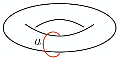

Using this fact, we can relate certain products of operators to the string-operator associated with the (doubled) anyon . That is, assume that the edges cover a topologically non-trivial loop on the (dual) lattice (e.g., in the -qudit torus of Fig. 4). Then we have
| (207) |
for some constant . This follows by comparing (206) with the graphical representation of the string-operators of the doubled model as discussed in [44], see Fig. 16. Note also that by the topological order condition, operators of the form are proportional to if .
B.2 Effective Hamiltonians for translation-invariant perturbation
According to (184) and (186), a translation-invariant perturbation of the form for the doubled semion or Fibonacci models (as considered in Section 7) is, up to a global energy shift and a proportionality constant, equivalent to a perturbation of the form
| (208) |
where and the sum is over all edges of the lattice (Here in the doubled semion model and in the Fibonacci model). We show the following:
Lemma B.3.
For the perturbation (208) to the Levin-Wen model , the -th order effective Hamiltonian is given by
| (209) |
where and are constants, and the sum is over all topologically non-trivial loops of length .
Proof.
According to Theorem 3.2, the -th order effective Hamiltonian is proportional to
| (210) |
up to an energy shift. By the topological order constraint, the only summands on the rhs. which can have a non-trivial action on the ground space are those associated with edges constituting a non-trivial loop on the (dual) lattice. Note that for such a collection of edges, every plaquette has at most two edges as its sides, a fact we will use below. Our claim follows if we show that for any such collection of edges, we have
| (211) |
for some constant .
We show (211) by showing that the resolvent operators only contribute a global factor; the claim then follows from (207). The reason is that the local operators create localized excitations, and these cannot be removed unless operators acting on the edges of neighboring plaquettes are applied. Thus a process as the one on the lhs. (207) is equivalent to one which goes through a sequence of eigenstates of the unperturbed Hamiltonian .
The proof of this statement is a bit more involved since operators can also create superpositions of excited and ground states. We proceed inductively. Let us set
| (212) |
such that
| (213) |
Let be a ground state of the Levin-Wen model . We claim that for every , there is a set of plaquettes and a constant (independent of the chosen ground state) such that
- (i)
.
- (ii)
The (unnormalized) state is an eigenstate of . Its energy is independent of the state .
- (iii)
The set only contains plaquettes which have two edges in common with .
Note that for , this implies because , and the claim (211) follows with (207)
Properties (i), (ii) hold for , with and : we have for any ground state
| (214) |
and this is an eigenstate of with energy according to Lemma B.1.
Assume now that (i), (ii) hold for some . Then we have according to (213)
| (215) | ||||
| (216) | ||||
| (217) | ||||
| (218) |
where
| (219) |
It hence suffices to show that for some choice of plaquettes , we have
- (a)
- (b)
is an eigenstate of with energy (independent of ).
- (c)
that the set only contains plaquettes sharing two edges with .
By assumption (iii) and the particular choice of , none of the plaquettes contains the edge . Therefore, we can commute the operator through, getting
| (220) |
We then consider two cases:
- •
- •
If there is an edge , such that and belong to the same plaquette , then the state (220) is a superposition of states with excited/not excited, that is, we have
(221) However, an excitation at cannot disappear by applying the operators since these do not share an edge with , hence (recall that includes a projection onto the ground space). Thus setting , we can verify that – indeed are satisfied. (The case where there are two such plaquettes can be treated analogously.)
∎
Let us compute the effective Hamiltonian (209) for the case of the rhombic torus, or more specifically, the lattice we use in the numerical simulation, Fig. 4. It has three inequivalent weight-2 loops: . Follow the recipe in Section 6.2, respectively Section 7.2, these three loops are related by a rotation. The corresponding unitary transformation for this rotation is given by the product of matrices when expressed in the flux basis discussed in Section 6.2 (for the doubled Fibonacci model, the latter two matrices are given by (93)). Similarly, we can express the action of in this basis using (68), getting a matrix . By (87), the effective Hamiltonian for the perturbation is then proportional to (when expressed in the same basis)
| (222) |
Note that the overall sign of the effective Hamiltonian is not specified in (65), but can be determined to be negative here by explicit calculation. For example, substituting in the matrix (Eq. (93)) of the doubled Fibonacci model, we have for the Fibonacci model. It is then straightforward to obtain the ground state of , which is
| (223) |
where is a flux basis vector, i.e., the image of (see Section 6.2) up to some phase.
References
- [1] A.A. Abrikosov, D.E. Brown, and I.E. Dzyaloshinsky. Quantum Field Theoretical Methods in Statistical Physics. Dover, New York, 1975.
- [2] P. W. Anderson. Absence of Diffusion in Certain Random Lattices. Physical Review, 109(5):1492–1505, mar 1958.
- [3] P. W. Anderson. Infrared Catastrophe in Fermi Gases with Local Scattering Potentials. Physical Review Letters, 18(24):1049, jun 1967.
- [4] CE Bardyn, MA Baranov, CV Kraus, E Rico, A İmamoğlu, P Zoller, and S Diehl. Topology by dissipation. New Journal of Physics, 15(8):085001, 2013.
- [5] Michael E. Beverland, Oliver Buerschaper, Robert König, Fernando Pastawski, John Preskill, and Sumit Sijher. Protected gates for topological quantum field theories. arXiv:1409.3898, 2014.
- [6] Sergey Bravyi, David P. DiVincenzo, and Daniel Loss. Schrieffer–wolff transformation for quantum many-body systems. Annals of Physics, 326(10):2793 – 2826, 2011.
- [7] Sergey Bravyi and Matthew B Hastings. A short proof of stability of topological order under local perturbations. Communications in mathematical physics, 307(3):609–627, 2011.
- [8] Sergey Bravyi, Matthew B Hastings, and Spyridon Michalakis. Topological quantum order: stability under local perturbations. Journal of Mathematical Physics, 51(9):093512, 2010.
- [9] S. Bravyi, M. B. Hastings, and F. Verstraete. Lieb-robinson bounds and the generation of correlations and topological quantum order. Phys. Rev. Lett., 97:050401, Jul 2006.
- [10] Maissam Barkeshli, Chao-Ming Jian, and Xiao-Liang Qi. Classification of topological defects in abelian topological states. Phys. Rev. B, 88(24):241103–, 12 2013.
- [11] Sergey Bravyi and Alexei Kitaev. Universal quantum computation with ideal clifford gates and noisy ancillas. Physical Review A, 71(2):022316, 2005.
- [12] Sergey Bravyi and Robert König. Disorder-assisted error correction in majorana chains. Communications in Mathematical Physics, 316(3):641–692, 2012.
- [13] Sergey Bravyi and Robert König. Classification of topologically protected gates for local stabilizer codes. Phys. Rev. Lett., 110:170503, Apr 2013.
- [14] R Barends, J Kelly, A Megrant, A Veitia, D Sank, E Jeffrey, T C White, J Mutus, A G Fowler, B Campbell, Y Chen, Z Chen, B Chiaro, A Dunsworth, C Neill, P O’Malley, P Roushan, A Vainsencher, J Wenner, A N Korotkov, A N Cleland, and John M Martinis. Superconducting quantum circuits at the surface code threshold for fault tolerance. Nature, 508(7497):500–3, apr 2014.
- [15] Claude Bloch. Sur la théorie des perturbations des états liés. Nuclear Physics, 6:329–347, 1958.
- [16] H. Bombin and M. A. Martin-Delgado. Quantum measurements and gates by code deformation. Journal of Physics A: Mathematical and Theoretical, 42(9):095302, 2009.
- [17] H. Bombin. Gauge color codes: optimal transversal gates and gauge fixing in topological stabilizer codes. New Journal of Physics, 17(8):083002, 2015.
- [18] Parsa Bonderson. Splitting the Topological Degeneracy of Non-Abelian Anyons. Physical Review Letters, 103(11):110403, 2009.
- [19] FA Bais and JK Slingerland. Condensate-induced transitions between topologically ordered phases. Physical Review B, 79(4):045316, 2009.
- [20] FJ Burnell, Steven H Simon, and JK Slingerland. Condensation of achiral simple currents in topological lattice models: Hamiltonian study of topological symmetry breaking. Physical Review B, 84(12):125434, 2011.
- [21] Salman Beigi, Peter W. Shor, and Daniel Whalen. The quantum double model with boundary: Condensations and symmetries. Commun. Math. Phys., 306(3):663–694, 2011.
- [22] Tommaso Caneva, Rosario Fazio, and Giuseppe E. Santoro. Adiabatic quantum dynamics of a random Ising chain across its quantum critical point. Physical Review B, 76(14):144427, oct 2007.
- [23] Jerry M Chow, Jay M Gambetta, Easwar Magesan, David W Abraham, Andrew W Cross, B R Johnson, Nicholas A Masluk, Colm A Ryan, John A Smolin, Srikanth J Srinivasan, and M Steffen. Implementing a strand of a scalable fault-tolerant quantum computing fabric. Nature communications, 5:4015, jan 2014.
- [24] A.D. Córcoles, Easwar Magesan, Srikanth J. Srinivasan, Andrew W. Cross, M. Steffen, Jay M. Gambetta, and Jerry M. Chow. Demonstration of a quantum error detection code using a square lattice of four superconducting qubits. Nature Communications, 6:6979, apr 2015.
- [25] Eric Dennis, Alexei Kitaev, Andrew Landahl, and John Preskill. Topological quantum memory. Journal of Mathematical Physics, 43(9):4452–4505, 2002.
- [26] John Dengis, Robert König, and Fernando Pastawski. An optimal dissipative encoder for the toric code. New Journal of Physics, 16(1):013023, 2014.
- [27] Michael Freedman, Alexei Kitaev, Michael Larsen, and Zhenghan Wang. Topological quantum computation. Bulletin of the American Mathematical Society, 40(1):31–38, 2003.
- [28] Adrian Feiguin, Simon Trebst, Andreas WW Ludwig, Matthias Troyer, Alexei Kitaev, Zhenghan Wang, and Michael H Freedman. Interacting anyons in topological quantum liquids: The golden chain. Physical Review Letters, 98(16):160409, 2007.
- [29] Alexander L Fetter and John Dirk Walecka. Quantum theory of many-particle systems. Courier Corporation, 2003.
- [30] Yimin Ge, András Molnár, and J Ignacio Cirac. Rapid adiabatic preparation of injective peps and gibbs states, 2015. arXiv:1508.00570.
- [31] Alioscia Hamma and Daniel A Lidar. Adiabatic preparation of topological order. Physical Review Letters, 100(3):030502, 2008.
- [32] A Hamma, W Zhang, S Haas, and DA Lidar. Entanglement, fidelity, and topological entropy in a quantum phase transition to topological order. Physical Review B, 77(15):155111, 2008.
- [33] Robert König and Ersen Bilgin. Anyonic entanglement renormalization. Physical Review B, 82(12):125118, 2010.
- [34] J Kelly, R Barends, AG Fowler, A Megrant, E Jeffrey, TC White, D Sank, JY Mutus, B Campbell, Yu Chen, et al. State preservation by repetitive error detection in a superconducting quantum circuit. Nature, 519(7541):66–69, 2015.
- [35] A Yu Kitaev. Unpaired Majorana fermions in quantum wires. Physics-Uspekhi, 44(10S):131, 2001.
- [36] A Yu Kitaev. Fault-tolerant quantum computation by anyons. Annals of Physics, 303(1):2–30, 2003.
- [37] Alexei Kitaev. Anyons in an exactly solved model and beyond. Annals of Physics, 321(1):2–111, 2006.
- [38] Alexei Kitaev and Liang Kong. Models for gapped boundaries and domain walls. Commun. Math. Phys., 313(2):351–373, 2012.
- [39] Robert König, Greg Kuperberg, and Ben W Reichardt. Quantum computation with Turaev–Viro codes. Annals of Physics, 325(12):2707–2749, 2010.
- [40] Emanuel Knill and Raymond Laflamme. Theory of quantum error-correcting codes. Physical Review A, 55(2):900–911, feb 1997.
- [41] Robert König and Fernando Pastawski. Generating topological order: no speedup by dissipation. Physical Review B, 90(4):045101, 2014.
- [42] Justyna Lodyga, Pawel Mazurek, Andrzej Grudka, and Michal Horodecki. Simple scheme for encoding and decoding a qubit in unknown state for various topological codes. Scientific reports, 5:8975, jan 2015.
- [43] Daniel A Lidar, Ali T Rezakhani, and Alioscia Hamma. Adiabatic approximation with exponential accuracy for many-body systems and quantum computation. Journal of Mathematical Physics, 50(10):102106, 2009.
- [44] Michael A Levin and Xiao-Gang Wen. String-net condensation: A physical mechanism for topological phases. Physical Review B, 71(4):045110, 2005.
- [45] Spyridon Michalakis and Justyna P. Zwolak. Stability of Frustration-Free Hamiltonians. Communications in Mathematical Physics, 322(2):277–302, jul 2013.
- [46] V Mourik, K Zuo, S M Frolov, S R Plissard, E P A M Bakkers, and L P Kouwenhoven. Signatures of Majorana fermions in hybrid superconductor-semiconductor nanowire devices. Science (New York, N.Y.), 336(6084):1003–7, may 2012.
- [47] Stevan Nadj-Perge, Ilya K Drozdov, Jian Li, Hua Chen, Sangjun Jeon, Jungpil Seo, Allan H MacDonald, B Andrei Bernevig, and Ali Yazdani. Topological matter. Observation of Majorana fermions in ferromagnetic atomic chains on a superconductor. Science (New York, N.Y.), 346(6209):602–7, oct 2014.
- [48] Chetan Nayak, Steven H Simon, Ady Stern, Michael Freedman, and Sankar Das Sarma. Non-abelian anyons and topological quantum computation. Reviews of Modern Physics, 80(3):1083, 2008.
- [49] R. N. C. Pfeifer, P. Corboz, O. Buerschaper, M. Aguado, M. Troyer, and G. Vidal. Simulation of anyons with tensor network algorithms. Physical Review B, 82(11):115126, sep 2010.
- [50] Pierre Pfeuty. The one-dimensional Ising model with a transverse field. Annals of Physics, 57(1):79–90, mar 1970.
- [51] Fernando Pastawski, Alastair Kay, Norbert Schuch, and Ignacio Cirac. Limitations of Passive Protection of Quantum Information. Quantum Information and Computation, 10(7&8):0580–0618, nov 2010.
- [52] Gustavo Rigolin and Gerardo Ortiz. Adiabatic Perturbation Theory and Geometric Phases for Degenerate Systems. Physical Review Letters, 104(17):170406, apr 2010.
- [53] Gustavo Rigolin and Gerardo Ortiz. Adiabatic theorem for quantum systems with spectral degeneracy. Physical Review A, 85(6):062111, jun 2012.
- [54] Gustavo Rigolin and Gerardo Ortiz. Degenerate adiabatic perturbation theory: Foundations and applications. Physical Review A, 90(2):022104, aug 2014.
- [55] Subir Sachdev. Quantum Phase Transitions. Cambridge University Press, 2011.
- [56] Marc Daniel Schulz. Topological phase transitions driven by non-Abelian anyons. PhD thesis, Technischen Universität Dortmund, 2013.
- [57] J. R. Schrieffer and P. A. Wolff. Relation between the anderson and kondo hamiltonians. Phys. Rev., 149:491–492, Sep 1966.
- [58] Stefan Teufel. Adiabatic perturbation theory in quantum dynamics. Springer-Verlag Berlin Heidelberg, 2003.
- [59] Vivek Venkatachalam, Amir Yacoby, Loren Pfeiffer, and Ken West. Local charge of the = 5/2 fractional quantum Hall state. Nature, 469(7329):185–8, jan 2011.
- [60] Zhengang Wang. Topological quantum computation, volume Regional Conference Series in Mathematics/Conference Board of the mathematical Sciences, no. 112. American Mathematical Society, 2010.
- [61] Beni Yoshida. Gapped boundaries, group cohomology and fault-tolerant logical gates. arXiv:1509.03626, 2015.
- [62] Beni Yoshida. Topological color code and symmetry-protected topological phases. Phys. Rev. B, 91(24):245131–, 06 2015.