A Hybrid Method and Unified Analysis of Generalized
Finite Differences and Lagrange Finite Elements
Abstract
Finite differences, finite elements, and their generalizations are widely used for solving partial differential equations, and their high-order variants have respective advantages and disadvantages. Traditionally, these methods are treated as different (strong vs. weak) formulations and are analyzed using different techniques (Fourier analysis or Green’s functions vs. functional analysis), except for some special cases on regular grids. Recently, the authors introduced a hybrid method, called Adaptive Extended Stencil FEM or AES-FEM (Int. J. Num. Meth. Engrg., 2016, DOI:10.1002/nme.5246), which combines features of generalized finite differences and Lagrange finite elements to achieve second-order accuracy over unstructured meshes. However, its analysis was incomplete due to the lack of existing mathematical theory that unifies the formulations and analysis of these different methods. In this work, we introduce the framework of generalized weighted residuals to unify the formulation of finite differences, finite elements, and AES-FEM. In addition, we propose a unified analysis of the well-posedness, convergence, and mesh-quality dependency of these different methods. We also report numerical results with AES-FEM to verify our analysis. We show that AES-FEM improves the accuracy of generalized finite differences while reducing the mesh-quality dependency and simplifying the implementation of high-order finite elements.
Keywords:
partial differential equations, finite element methods, generalized finite differences, generalized weighted residuals, stability, convergence2010 MSC
65N06 , 65N30 , 65N121 Introduction
Finite differences, finite elements, and their generalizations are widely used for solving partial differential equations (PDEs), or more precisely, for the spatial discretization for their associated boundary value problems (BVPs). The finite difference methods (FDM) are standard techniques in numerical analysis [1, 2] and are widely used for solving hyperbolic PDEs in computational fluid dynamics. The finite element methods (FEM), on the other hand, are the most successful method for solving elliptic and parabolic PDEs (e.g., [3, 4]). Since many PDEs, such as advection-diffusion-reaction equations, Navier-Stokes equations, etc., are multiphysics in nature, involving both parabolic (elliptic) and hyperbolic components, it has been of great interest for applied mathematicians to develop hybrid methods that combine the advantages of FEM and FDM. The most notable examples are discontinuous Galerkin methods [5, 6] and some finite volume methods [7, 8], which use discontinuous test functions analogous to the nonconforming finite elements [9, Section 10.3] and use finite-difference style computations of interface fluxes or jump conditions (such as WENO [10, 11] and Lax–Friedrichs limiters [7, p. 199]) along element or cell boundaries.
In [12, 13], the authors introduced a new hybrid method, called the adaptive extended stencil finite element method or AES-FEM. Like Lagrange finite elements, AES-FEM has continuous test functions, so there are no explicit interface and jump conditions in its variational forms, unlike nonconforming finite elements. However, unlike finite elements, AES-FEM uses least-squares based trial functions similar to those of generalized finite differences [14]. We refer to these trial functions as generalized Lagrange polynomial (GLP) basis functions, which are not continuous but have similar properties to Lagrange interpolation. The GLP basis functions introduce a “variational crime” (cf. D.3), which is similar to, but yet different from, that of other nonconforming finite elements. The analysis of GLP-based methods, including generalized finite difference method (GFDM) and AES-FEM, requires a mathematical analysis that unifies the classical analysis of finite differences and finite elements. This unification is the primary goal of this work, which will reveal some insights from a theoretical point of view, and also enable a rigorous generalization of AES-FEM to higher-order accuracy from a practical point of view.
The main contributions of this work are as follows. First, we unify the formulations of GFDM, FEM, and AES-FEM under the framework of generalized weighted residuals (GWR), of which the trial functions are either Lagrange or generalized Lagrange basis functions. Second, we establish the conditions for well-posedness, convergence, and superconvergence of GFDM and AES-FEM, and compare their mesh-quality requirements against Lagrange finite elements. Third, we prove and also demonstrate the high-order convergence of AES-FEM. For simplicity, we assume exact geometry for Neumann boundaries in this paper, and we defer the treatment of Neumann boundary conditions over approximate curved boundaries to future work.
The remainder of the paper is organized as follows. Section 2 reviews the (G)FDM and FEM for boundary value problems, as well as their respective classical analyses. Section 3 introduces the concept of generalized Lagrange polynomial basis functions and the framework of generalized weighted residuals (GWR), which unifies the formulations of GFDM, FEM, and AES-FEM. Section 4 analyzes the well-posedness of GWR methods. Section 5 addresses the convergence of GFDM and AES-FEM to confirm our analysis. Section 6 presents some numerical results. Section 7 concludes this paper with a discussion on future work.
2 Background and Preliminaries
In this section, we briefly review finite differences, finite elements, and some of their generalizations for boundary value problems. We refer readers to [15] for a brief history of these different methods. For completeness, we review some relevant details about the generalized Lagrange polynomials, AES-FEM, and functional analysis in the appendices.
2.1 Boundary Value Problems
Let be a bounded, piecewise smooth domain with boundary , where is typically 2 or 3, and and denote the Dirichlet and Neumann boundaries, respectively. Let be a second-order linear differential operator. In general, has the form of
| (2.1) |
where and denote the gradient and divergence operators, corresponds to a diffusion coefficient, is a velocity field, and is a wavenumber or frequency. Typically, . A second-order partial differential equation has the form of
| (2.2) |
where is a source term. This general form is known as the advection-diffusion-reaction equations for vector-valued PDEs. For simplicity, we focus on scalar fields and assume diffusion dominance (i.e., for some , where denotes some characteristic edge length of the mesh; cf. D). If , then its corresponding PDE is the advection-diffusion equation. A boundary value problem (BVP) corresponding to the above PDE may have some Dirichlet boundary conditions
| (2.3) |
and potentially some Neumann boundary conditions
| (2.4) |
where denotes the normal derivative, i.e., . The boundary condition is said to be homogeneous if and .
2.2 Finite Differences and Their Generalizations
The finite difference methods (FDM) are arguably the simplest and the best known numerical methods for solving initial and boundary value problems; see textbooks such as [1, 2]. In a nutshell, FDM approximates the partial derivatives in (2.1) using finite difference operators, which result in a system of algebraic equations . The analysis of FDM is also conceptually simple: If the truncation errors in each algebraic equation are consistent (i.e., for some as the edge length tends to ) and the absolute condition number of the algebraic system (i.e., ) is bounded independently of (i.e., ), then the finite difference method converges in exact arithmetic. This condition is known as the fundamental theorem of numerical analysis and is simply stated as “consistency and stability imply convergence” [3, p. 124]. The main argument then involves bounding the absolute condition number, which traditionally is done using Fourier analysis on regular grids [1, p. 20] or using Green’s functions in 1D [1, p. 22]. The effect of rounding errors is typically omitted in the analysis of BVPs, but it has been considered by some authors; see e.g. [16, 17, 18].
The classical FDM is limited to structured meshes because the finite difference operators are defined based on 1D polynomial interpolations locally at each node in a dimension-by-dimension fashion. The same approach can be utilized on curvilinear meshes for curved but relatively simple geometries; see e.g. [19]. Some authors have considered its generalizations to unstructured meshes or point clouds; see e.g. [14, 20, 21, 22]. Finite difference operators have been generalized to use least-squares approximations; see e.g. [14, 20, 21]. In this work, we use generalized finite differences (GFD) to refer to the least-squares-based finite difference operators and use generalized finite difference methods (GFDM) to refer to the methods that use these GFD operators to convert (2.2) directly into algebraic equations. To the best of our knowledge, there was no prior complete convergence analysis of GFDM for BVPs, except for local consistency using Taylor series and the temporal aspect of stability for time-dependent PDEs [14, 23, 24, 25].
2.3 Finite Elements and Weighted Residuals
The finite element methods (FEM) are among the most powerful and successful methods for solving BVPs. Mathematically, FEM can be expressed using the framework of weighted residuals [26], also known as variational formulations [9, p. 2]. Let denote the approximation of the domain with a mesh. Without loss of generality, let us assume triangular or tetrahedral meshes, and let denote the number of nodes in . Let denote the approximate solution of the PDE on . The residual of (2.2) corresponding to is . Let denote the set of test (or weight) functions, which span the test space . A weighted residual method requires the residual to be orthogonal to over , or equivalently,
| (2.5) |
In FEM, the test functions are (weakly) differentiable and have local support.
To discretize the problem fully, let denote a set of basis functions, which span the trial space . Let denote the vector containing . We find the approximate solution in , i.e.,
| (2.6) |
where is the unknown vector. The basis functions are Lagrange if , the Kronecker delta function; i.e., if and if . With Lagrange basis functions, let denote the vector composed of . Then, is the interpolation of in . Furthermore, the unknown vector in (2.6) is composed of approximations to nodal values . The FEM using Lagrange basis functions is called Lagrange FEM [27, p. 36]. In this work, FEM refers to Lagrange FEM, unless otherwise noted.
For elliptic PDEs, FEM solves (2.5) by performing integration by parts and then substituting the boundary conditions (2.3) and (2.4) into the resulting integral equation. Let denote the inner product over ,11 1 In functional analysis, the inner product is denoted as . We use for clarity and for distinguishing the inner products on and on boundary . See D for a review of some relevant functional analysis concepts. i.e.,
| (2.7) |
which defines the norm over , i.e., . Similarly, let denote the inner product over . For the general linear operator in (2.1), after integration by parts of the first term, we obtain a variational form for each test function
| (2.8) |
where
| (2.9) |
is the bilinear form.
2.4 Prior Efforts on Unified Analysis of FDM and FEM
The unification of the accuracy and stability analysis of FDM and FEM has been of great interest to numerical analysts since the late 1960s [28, 3]. In terms of local error analysis, this unification is straightforward by using Taylor series, except that FDM traditionally relied on 1D Taylor series, whereas FEM requires the higher-dimensional version. In terms of global error analysis, Fix and Strang explored adapting Fourier analysis from FDM to FEM on structured grids [28]. Another common technique used in analyzing both FDM and FEM is the Green’s functions. It was particularly successful for proving the convergence of FDM and superconvergence of FEM in norm in 1D or with tensor-product elements; see, e.g., [29, 30, 1]. In this work, we unify the analysis of well-posedness of GFDM, FEM, and AES-FEM by integrating functional analysis and approximation theory.
3 Generalized Weighted Residuals
To unify the formulations and analysis of GFDM, FEM, and AES-FEM, we need a mathematical framework that is more general than weighted residuals. The framework, which we refer to as generalized weighted residuals (GWR), has three components: a mesh and its associated test functions and geometric realization, a set of (generalized) Lagrange basis functions, and a (generalized) variational form. We address these three components using GFDM and FEM as examples, and then introduce AES-FEM under this framework.
3.1 Component 1: Meshes, Test Functions, and Geometry
3.1.1 Meshes
Like in FEM, in GWR the domain is tessellated by a mesh, which is typically simplicial or rectangular. Without loss of generality, we assume simplicial meshes in this work, which are triangular in 2D or tetrahedral in 3D. The triangles and tetrahedra are known as the elements, of which the vertices are called the nodes. Let denote the union of the geometric realizations of the elements, and let denote its boundary. Let denote an approximation of . We assume is the same as . Let , where denotes the interior of , denotes the approximation to the Dirichlet boundary, and . We refer to the nodes in , , and as interior, Neumann, and Dirichlet nodes, respectively. Without loss of generality, we assume the nodes are numbered between and , where the first nodes are those in .
3.1.2 Test Functions
In GWR, there is a test function associated with each node , analogous to those in (2.5). Each test function has local support, denoted by , which is the closure of the subset of points in such that , i.e., . Topologically, the local support is compact, in that it contains only a small constant number of nodes. In a Lagrange FEM, each test function is a Lagrange basis function, such as a hat (a.k.a. pyramid) function. Note that the test functions in FEM may be quadratic or higher-degree polynomials, which have mid-edge, mid-face, and mid-cell nodes, besides the corner nodes. For FEM, the local support is composed of the union of the elements incident on . For GFDM over an unstructured mesh, within the GWR framework, the test function at is the Dirac delta function at , and the local support of a Dirac delta function is itself. We will discuss this further in Section 3.3.
Remark 1
In [27], Ciarlet defined a finite element method as a triplet: a mesh, element-based (nearly) polynomial basis, and node-based basis functions of an space. A GWR is more general in that the test functions may not span an or space, which is the case in (generalized) finite difference methods.
3.1.3 Geometric Realizations
For numerical computations, the local support must have a geometric realization, which is the union of the geometric realizations of its elements. For each element , its geometric realization is defined through a mapping from a master element in the parametric space to the “physical space” . Let denote the natural coordinates in the parametric space. Let denote the number of nodes in , and let and denote the natural coordinates and physical coordinates, respectively, of the th node in , where . For example, a linear triangle has nodes , and . The geometric realization of an element is defined by a Lagrange interpolation
| (3.1) |
where is the local nodal ID in for the th node in . The functions are in general polynomials. Using the interpolation theory [34], given nodes and an equal number of monomials in , if the Vandermonde system in the parametric space is stable, then the basis functions are uniquely determined over . In FEM, the geometric basis functions do not need to be the same as the test functions (and trial functions ).
Besides the local support, we also define a “control volume” for each node to facilitate the theoretical analysis in Section 4 by generalizing its traditional definition. Let denote the Lebesgue measure (namely, the area or volume) of . The control volumes of all the nodes partition , i.e., and if . For FEM, the control volume of a node can be defined by the union of its closest points within its incident elements. For GFDM, we define the control volume similarly or use the Voronoi cells. Note that these control volumes are not used in computations; instead, we will use them in analyzing well-posedness and convergence. See Figure 7 in B for an example of a control volume.
3.1.4 Approximation Power of Lagrange Finite Elements
In FEM, the test (and trial) functions are Lagrange functions, which are defined using a mapping from a parametric space to the physical space , similar to that of the geometric basis functions. More precisely, let denote the Lagrange polynomial basis over the master element, which satisfies the Kronecker delta property . Let denote the mapping from the parametric space to the physical space and denote its inverse mapping. A global test function is then defined as
| (3.2) |
where is the local ID of node in . By construction, is a Lagrange test function over . A (piecewise) smooth function can be interpolated by the basis functions over by
| (3.3) |
If is piecewise linear, then the Lagrange test functions are polynomials. However, if is nonlinear, then are no longer polynomials. Nevertheless, is approximated to within each element if both and are bounded for [35], where denote the th derivative tensor and is an edge length measure.
3.2 Component 2: Generalized Lagrange Trial Functions
In GWR, for each node (and more generally, at each point) in , there is a set of generalized Lagrange trial functions, which may or may not be polynomials, and which may be interpolation (such as in FEM) or least-squares-based (such as in GFDM).
3.2.1 Generalized Lagrange Basis Functions
Definition 1
A set of functions form a set of generalized Lagrange basis functions of degree- consistency over local support with a stencil if
| (3.4) |
for a sufficiently differentiable function and , where is the radius of the stencil. These basis functions are stable over if for .
In the above, the “radius” is a local length measure of the stencil, and it can be replaced by other characteristic length measures, such as the maximum distance between the points in the stencil. This definition preserves two fundamental properties of degree- Lagrange basis functions: when approximating a function , the coefficient for each is , and is approximated to consistency. In FEM, consistent Lagrange trial (or test) functions constitute a set of generalized Lagrange basis functions.
3.2.2 Generalized Lagrange Polynomials
In GFDM, the derivatives are approximated using polynomials constructed using least squares approximations. We can express them in terms of generalized Lagrange polynomial (GLP) basis functions.
Definition 2
Given a stencil , degree- polynomials form a set of generalized Lagrange polynomial (GLP) basis functions if every degree- polynomial is interpolated exactly by .
In practice, the GLP basis functions are computed from the pseudoinverse solution of a Vandermonde system; see e.g. [12]. For completeness, we describe the procedure in A. If the Vandermonde matrix is nonsingular, i.e., the number of points in the stencil is equal to the number of monomials of up to degree and the stencil is not degenerate, then a set of GLP basis functions reduces to a set of Lagrange polynomial basis functions, which are commonly used in the classical finite difference methods. The basis functions are stable if the Vandermonde matrix is well conditioned. More importantly, they are generalized Lagrange trial functions.
The GLP basis functions are not unique in general in that they depend on how different points are weighted. For the AES-FEM results in Section 6, we use an inverse-distance-based weighting scheme given in (A.4). This weighting scheme tends to promote error cancellations on nearly symmetric meshes [36] and in turn improve accuracy [37]. We defer a detailed analysis to future work.
Lemma 1
Given a set of stable degree- GLP basis functions over , if is continuously differentiable up to th order, then (3.4) holds.
Proof 1
We note that there are some differences between the Lagrange basis functions in FEM and the GLP basis functions. First, the GLP basis functions are least-squares based, so they, in general, do not satisfy the Kronecker delta property, i.e., . Second, the Lagrange basis functions in FEM are continuous, whereas the GLP basis functions are quasicontinuous in that they are smooth over the local support, but they do not vanish exactly along the boundary. We illustrate these differences in Figure 1, which shows (a) a 2D FEM hat function, (b) a 2D quadratic GLP basis function at a node over the same stencil, and (c) a set of GLP basis functions at a node in 1D. Third, Lagrange basis functions in FEM are defined based on a mapping between the reference domain to the physical domain, and hence they depend on element shapes and are in general not polynomials with nonlinear geometric realizations, whereas the GLP basis functions do not depend on the element shapes and are true polynomials. Finally, the GLP basis functions are defined locally at a node (or a center point), and they do not necessarily define a global set of trial functions over . For these reasons, GWR requires a more general variational form than that used in FEM.

(a) A piecewise linear Lagrange
basis function in 2D.

(b) A quadratic GLP
basis function in 2D.

(c) A set of quadratic GLP
basis functions in 1D.
3.3 Component 3: Generalized Variational Form
Consider a node , and let denote the test function associated with . Let denote the vector containing the trial functions associated with the node . Let and denote the subvectors of corresponding to the nodes in and , respectively, i.e., and in MATLAB-style colon-notation. Let and be composed of the nodal values associated with and , respectively. In GWR, we approximate the solution of (2.2) locally about by
| (3.7) |
Let us first consider a BVP with Dirichlet boundary conditions. We define a generalized variational form (GVF) corresponding to (2.2) for an interior node as
| (3.8) |
where
| (3.9) |
is the generalized bilinear form associated with . Here, the inner product is computed over the local support of . These forms are “generalized” in that may be a generalized function (such as a Dirac delta function). Note that if vanishes along , the bilinear form in (2.9) and the generalized bilinear form (3.9) are mathematically equivalent to each other due to Green’s identities. Computationally, however, (2.9) requires to be at least and (3.9) requires to be at least .
3.3.1 Generalized Variational Form of GFDM
In (G)FDM, since the test functions are Dirac delta functions, which are not , we must use (3.9) instead of (2.9) computationally. Neumann boundary conditions can be incorporated into the generalized variational form; see [1, p. 31] for derivations of second-order FDM in 1D. Alternatively, one-sided differences can be used to convert (2.4) directly into an algebraic equation at each Neumann node [1, p. 32].
3.3.2 Variational Form of Lagrange FEM
For a Lagrange FEM with strongly imposed Dirichlet boundary conditions, its variational form is also a GVF. Since the trial functions are , we must use the bilinear form (2.9) computationally for . For BVP with Neumann boundary conditions, assuming accurate geometry, one can substitute into (2.8) for each node in , which weakly imposes Neumann boundary conditions (2.4).
3.4 Adaptive Extended Stencil FEM
Adaptive Extended Stencil FEM or AES-FEM, is a GWR method that combines the features of GFDM and FEM. In particular, AES-FEM uses a piecewise linear FEM mesh, and its associated hat functions as test functions in the interior. Its trial functions are the GLP trial functions. We say that an AES-FEM is degree- if its trial functions are degree- GLP basis functions at each node (or more generally, at each point). Because of the least-squares nature of GLP basis functions, the number of nodes in the stencil can be chosen adaptively to ensure the well-conditioning of the Vandermonde matrix. This is the reason for the name “adaptive extended stencil” in AES-FEM; we describe the selection of the stencils and its adaptation in B. Because the test functions are and the trial functions are differentiable to th order, we can use either (2.9) or (3.9) computationally, which would give the same results up to machine precision.
In [12], the authors considered quadratic AES-FEM and showed its second-order accuracy with Dirichlet boundary conditions. The focus of this work is to establish the well-posedness and convergence of higher-degree AES-FEM for Neumann boundary conditions over polygonal domains. As in FEM, we can substitute into (2.8) for each node in for AES-FEM. For curved domains, Neumann boundary conditions can be imposed using higher-order boundary representations similar to [39], as described in Section 3.1.4, or using Dirac delta test functions and one-sided differences as in GFDM. In this work, we assume polygonal domains and impose Neumann boundary conditions weakly as in FEM. We defer the analysis and comparison of different techniques for imposing Neumann conditions over curved boundaries to future work.
Remark 2
GFDM requires a cloud of nodes, rather than a mesh with elements, so it is considered a meshless method. However, to construct the stencils (a.k.a. stars), one needs a data structure, such as a quadtree/octree [40]. Because AES-FEM involves integration (see C), we use a mesh and an associated data structure to construct the stencils and to provide the elements for integration. The use of integration allows AES-FEM to enjoy additional error cancellations and hence better accuracy than GFDM on nearly symmetric meshes, as demonstrated in Section 6.
4 Well-Posedness in Norm
We first establish the well-posedness, and more precisely, algebraic invertibility, of generalized weighted residual methods for elliptic BVPs. Like that of FEM [41], this invertibility implies the existence and uniqueness of a solution in exact arithmetic. We focus on AES-FEM while making the analysis general enough for GFDM. In Section 5, we will establish the convergence of AES-FEM in the presence of rounding errors.
4.1 Algebraic Equations of GWR
To analyze a GWR method, we first convert its GVF into a system of linear equations. For generality, we assume the bilinear form (2.9), with strongly imposed Dirichlet boundary conditions and weakly imposed Neumann boundary conditions. For GFDM, we assume only Dirichlet boundary conditions, and the GVF is evaluated with (3.9) instead of (2.9).
From (2.9), we obtain an linear system in , namely,
| (4.1) |
where the th row of and are
| (4.2) | ||||
| (4.3) |
respectively. For the Poisson equation, is the stiffness matrix and is the load vector in FEM. For generality, we simply refer to as the coefficient matrix. Another important matrix is the mass matrix, which is the coefficient matrix of the constrained projection associated with the GWR,
| (4.4) |
where the th row of and are
For Galerkin FEM, the constrained projection is known as the projection [41, p. 132]. Note that Neumann constraints are not imposed explicitly in the constrained projection because they are satisfied weakly automatically.
4.2 Algebraic Error Analysis in Norm
To analyze the solutions of (4.1), we consider the nodal values in norm. Given a vector , its norm is , where . Note that this is independent of, and different from, the degree of the basis functions. We will primarily use the or norm (i.e., or ). The norm of is .
Let denote the solution vector of a GWR method on a mesh with nodes. Let denote the vector composed of . The error vector is
| (4.5) |
Consider the linear system (4.1). Its residual vector is
| (4.6) |
Suppose is nonsingular, and assume exact arithmetic. Then,
| (4.7) |
where is the absolute condition number in -norm of the linear system (4.1). Note that given and , .
4.3 Well-Posedness of Constrained Projection in Norm
We first apply backward error analysis to the constrained projection (4.4). It is an important base case for the analysis of elliptic PDEs. In particular, consider a perturbation to in the right-hand side of (4.4). This leads to a perturbation in . From (4.7), the perturbation in is bounded by
| (4.8) |
If is continuous, , so if ; on the other hand, if for some , an continuous perturbation in the right-hand side of (4.4) may lead to an perturbation in in norm. Hence, to be consistent with the classical Hadamard’s notion of well-posedness of variational methods [41, p. 82], we define a well-posed constrained projection as follows.
Definition 3
A constrained projection is well-posed in norm for independently of if it is well-conditioned, i.e.,
| (4.9) |
In practice, the well-posedness requires quasiuniform meshes.
Definition 4
A type of GWR meshes is quasiuniform if the ratio of the largest and smallest control volumes of the test functions is bounded independently of mesh resolution, i.e., .
For FEM, Definition 4 is satisfied with the classical definition of quasiuniform meshes (e.g., [9, 3]), which requires the ratio between the largest and smallest elements to be bounded. Definition 4 is more general and also applies to GFDM, of which the control volumes have nonzero measures, but the local support of a Dirac delta function has a zero measure; see Remark 3. For AES-FEM, we note the following fact.
Theorem 2
Constrained projection by AES-FEM is well-posed in norm for on a sufficiently fine quasiuniform mesh with consistent and stable GLP basis functions and test functions.
This theorem is similar to that of the well-posedness of projections [41, p. 387], but there are two complications. First, the GLP basis functions are not global basis functions over , so we cannot use functional analysis directly. Second, Theorem 2 is not limited to norms, so we cannot use eigenvalue analysis either. To address the first issue, we define a global basis function by blending the GLP basis functions using to obtain a basis function, i.e., , which is composed of
| (4.10) |
These blended basis functions have the same approximation order as the GLP basis functions [42], and hence
| (4.11) |
To overcome the second issue, we make use of Singer’s representation theorem [43]. We omit the detailed proof, which is similar to that of Theorem 3 below.
4.4 Well-Posedness for Elliptic BVPs
Consider a perturbation to in the right-hand side of (4.4). This leads to a perturbation in , where . From (4.7), the perturbation in is bounded by
| (4.12) |
Hence, if . On the other hand, if for some , an continuous perturbation in the right-hand side of (4.4) may lead to an perturbation in in . Hence, we define well-posedness as follows.
Definition 5
For AES-FEM, we note the following theorem.
Theorem 3
Given an elliptic BVP, AES-FEM is well-posed in norm for on a sufficiently fine quasiuniform mesh with consistent and stable GLP basis functions and test functions.
Similar to Theorem 2, the proof requires an adaptation by using to construct a approximation in order to apply Singer’s representation theorem. Similar to the Lax-Milgram lemma, the proof also involves an assumption of invertibility of the PDE in infinite dimensions, and a boundedness assumption due to Friedrichs’ inequality [9, p. 104], which is more general than the Poincaré inequality [41, p. 489]. For completeness, we give the proof as follows.
Proof 2
Let and . Let denote Hölder’s conjugate of , i.e., , and let . Since is continuous, due to Singer’s representation theorem, there exists a solution such that . If the PDE is invertible in infinite dimensions,
| (4.14) |
Due to Friedrichs’ inequality, and . Furthermore, , Hence,
| (4.15) |
On a quasiuniform mesh,
| (4.16) |
Since ,
| (4.17) |
Since ,
| (4.18) |
and
| (4.19) |
Let , where is composed of nodal solutions of AES-FEM and is composed of the interpolated nodal values. It is easy to see that the above proof also applies to FEM, simply by replacing with the Lagrange basis functions in the proof. Hence, Theorems 2 and 3 both apply to FEM.
Remark 3
We can generalize Theorems 2 and 3 to GFDM as follows. Let and , where is a diagonal matrix with . Let denote the vector of hat functions over the mesh. Then, it is easy to show that and . By replacing with , the proof for Theorem 3 applies to GFDM with Dirichlet boundary conditions; similarly for Theorem 2.
4.5 Mesh Dependency for Well-Posedness
From the preceding analysis, it is clear that all the GWR methods have some level of dependency on meshes. In particular, all the methods require the quasiuniformity of control volumes of the nodes. For FEM and AES-FEM, this is equivalent to the quasiuniformity of the local support of the test functions. For GFDM, although the computation does not depend on a mesh, the quasiuniformity imposes restrictions on the distributions of the nodes.
Besides quasiuniformity, FEM requires well-shaped elements, because the Lagrange trial and test functions are based on the transformation from the parametric space to the physical space. For linear elements over polytopal domains, the well-shapedness requires the angles within the elements to be bounded away from and 0 [44, 45], which is needed for the stability of interpolations and derivative approximations. If some elements contain angles that are too small, the stiffness matrix in FEM may become ill-conditioned [46]. For high-order elements, the nodes must be well-positioned within the master elements so that the Lagrange basis functions are stable. In contrast, the well-posedness of GFDM does not depend on element shapes, but the stability of the GLP basis functions does depend on the selection of the stencils. Similarly, AES-FEM also depends on the stencils for the stability of its trial functions. However, the stencils in GFDM and AES-FEM can be adapted more easily due to their least squares nature. If the generalized bilinear form (3.9) is used, then AES-FEM also depends on the stability of the Lagrange test functions in the parametric space, but it does not require well-shaped elements in the physical space. If the bilinear form (2.9) is used over linear elements, then (2.9) is equal to (3.9) to machine precision, and hence there is no dependency on element shape either. In addition, high-order AES-FEM requires only first-order meshes for its implementation at least in the interior of the domain, so its implementation is simpler than that of high-order finite elements, which requires high-order meshes.
For geometries with curved boundaries, Lagrange FEM typically uses isoparametric elements, for which the well-posedness depends on the Ciarlet-Raviart condition [35]. Assuming stable Lagrange basis functions, the Ciarlet-Raviart condition requires the th derivatives for the mapping from the physical space to the parametric space to be bounded for , i.e., for in the master element. Mathematically, this condition is needed due to the high-order chain rule, also known as the Faà di Bruno’s formula [47],
| (4.21) |
where , , , denotes the derivative tensor of order , and “” denotes the scalar product of th-order tensors. For AES-FEM, if (3.9) is used with a higher-order boundary representation, then the Ciarlet-Raviart condition is also required when computing . However, the generalized bilinear form (3.9) uses only over the master element, so the Ciarlet-Raviart condition is no longer required. In this case, however, AES-FEM requires imposing Neumann boundary conditions similar to the techniques in GFDM instead of FEM. The well-posedness and consistency of such a hybrid treatment over curved boundaries require a more general analysis, and we defer it to future work.
5 Convergence in Norm
In this section, we analyze the convergence of GWR methods in norm. Given a vector of nodal errors , the convergence rate in norm is th order if , where is some edge length measure of a quasiuniform mesh.
5.1 Convergence of GWR Methods for Constrained Projection
Let , where and are the projected and interpolated nodal values. We then obtain the following result regarding the convergence of the constrained projection.
Theorem 4 (Convergence of constrained projection)
Under the same assumptions as in Theorem 2, if is continuously differentiable to th order within each element, the solution of the constrained projection with a well-posed degree- GWR method converges at or better in norm, i.e., .
Proof 3
Let . Due to the consistency of GLP basis functions, , so
| (5.1) |
The theorem also applies to other norms. In Theorem 4, we use “” sign to emphasize that the bound may not be tight due to possible superconvergence. Note that Theorem 4 applies to FEM, GFDM, and AES-FEM. For all of these methods, if is even, the leading error term in the residual is odd order, which may cancel out in the integration. In turn, it may lead to superconvergence. The superconvergence of FEM for the projection was considered in [48].
5.2 Convergence of GWR Methods for Elliptic BVPs
Let denote the nodal solutions of (4.1) corresponding to the nodes in . Let . We first give a loose error bound using an argument similar to that of Theorem 4. We state the bound in norm, but the result also holds in any norm for .
Lemma 5
Under the same assumptions as in Theorem 3, assuming exact arithmetic, the solution with a well-posed degree- GWR method for an elliptic BVP converges at or better in norm, i.e., .
Proof 4
Let . Using the same argument as for Lemma 1, it is easy to show that for . Hence, , and
| (5.2) |
Remark 4
For FEM, Lemma 5 underestimates the convergence rate by two orders, compared to the well-known error bounds in norm due to the Aubin-Nitsche duality argument; see e.g. [3]. The derivation of error bounds for FEM in norm is beyond the scope of this work. For GFDM and AES-FEM, however, the Aubin-Nitsche duality argument does not apply, due to the non-conformity. For odd-degree- GFDM and AES-FEM, Lemma 5 is tight. However, for even-degree-, similar to constrained projections, the leading error term in the residual is odd order, which may cancel out in the integration. For GFDM, this error cancellation occurs with symmetric stencils, analogous to centered differences, leading to convergence rate. With AES-FEM, however, the error cancellation is primarily due to the numerical integration, for example, see Figure 4.
Theorem 6
Under the same assumptions as in Theorem 3, assuming exact arithmetic, the solution of a well-posed even-degree- AES-FEM for a coercive elliptic BVP with Dirichlet boundary conditions converges at in norm, if or if and the local support is nearly symmetric.
Proof 5
Let denote the local interpolation at a node . Let , which is a smooth function over . Apply to . We note that
| (5.3) |
where is proportional to . If , because is the hat function, the line integral of cancels out exactly, so in Lemma 5. For even , the line integral cancels out if the local support is (nearly) symmetric about .
In [12], quadratic AES-FEM was shown to converge at second order, but the proof did not explicitly state the error cancellation. Theorem 6 indicates that AES-FEM may not enjoy the full superconvergence for on highly irregular meshes, but in practice we observe it to be close to on quasiuniform meshes, as we will demonstrate in Section 6.2.
6 Numerical Results
In this section, we present some numerical results to verify the theoretical analysis in this work.
6.1 Comparison of Mesh Dependency
We first compare the mesh dependency of FEM to that of AES-FEM. As shown in Section 4.5, the well-posedness of FEM depends on well-shapedness of the meshes, while AES-FEM is independent of element shapes, regardless of the degree of the GLP basis functions. To demonstrate this, we solved the Poisson equation in 2D
| (6.1) |
with Dirichlet boundary conditions over . We obtained and from the exact solution and solved the equation using our own implementations of quadratic, quartic, and sextic AES-FEM, along with linear, quadratic, and cubic FEM. We generated a series of meshes on a unit square with progressively worse element quality, which we obtain by distorting a good-quality mesh. For AES-FEM and linear FEM, we used a mesh with 130,288 elements and 65,655 nodes and distorted four elements by moving one vertex of each of these elements incrementally towards its opposite edge. For quadratic FEM, the mesh had 32,292 elements and 65,093 nodes, and a single element was distorted by moving one vertex and its adjacent mid-edge nodes incrementally towards its opposite edge. For cubic FEM, the mesh had 32,292 elements and 146,077 nodes, and also a single element was distorted. Figure 3 shows the condition numbers of the stiffness matrices of FEM and AES-FEM.
In practice, the condition number may affect the efficiency of iterative solvers. Figure 3 shows the numbers of iterations required to solve the linear systems to a relative tolerance of using GMRES for AES-FEM and CG for FEM, both with Gauss-Seidel preconditioners. It can be seen that the condition numbers of FEM increased inversely proportional to the minimum angle, and the number of iterations of CG grew correspondingly. In contrast, the condition numbers and the number of iterations for AES-FEM remained constant. We observed similar behavior for 3D AES-FEM, which we omit from the paper.


6.2 Convergence of High-Order AES-FEM
Next, we verify the convergence analysis in Section 5.2, especially that of AES-FEM. To this end, we used AES-FEM of degrees 2 to 6 to solve the equation
| (6.2) |
with unstructured meshes over , where . Figure 4(a) shows the convergence rates in the relative norm for the Poisson equation, for which . Figure 4(b) and (c) show the convergence rates for the advection-diffusion equation with Dirichlet and Neumann boundary conditions, respectively, where . The number to the right of each convergence curve shows the average convergence rate under mesh refinement. Note that AES-FEM with even-degree basis functions converged at about th order whereas with odd-degree basis functions, AES-FEM converged at st order. For example, with quadratic and cubic basis functions, the convergence rate is approximately second order. This difference in convergence rates is due to error cancelation in the numerical integration, as discussed in Section 5.2.
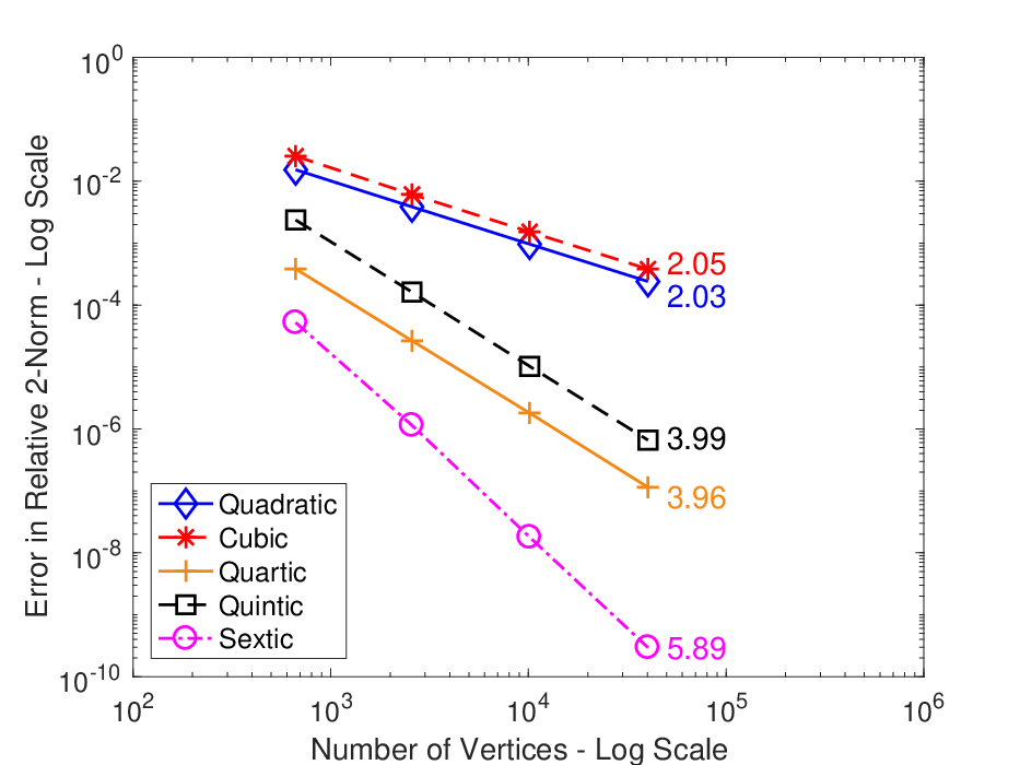
(a) Poisson equation
with Dirichlet boundaries.
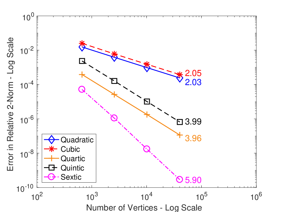
(b) Advection-diffusion equation
with Dirichlet boundaries.

(c) Advection-diffusion equation
with Neumann boundaries.
6.3 Comparison of FEM, GFDM, and AES-FEM
Finally, we compare the accuracy of FEM, GFDM, and FEM. We use the Poisson equation in this comparison. In particular, we solved a 2D Poisson equation (6.1) over the square with an elliptical hole of semi-axes and in the middle. The domain, as illustrated in Figure 5(a), has nonuniform curvature along the inner boundary and has corners along the outer boundary. We applied Neumann boundary conditions to the outer boundary and applied Dirichlet boundary conditions to the inner boundary. We obtained the source term and the boundary conditions by differentiating the following analytic function
| (6.3) |

(a) Test domain.

(b) Low-order methods.

(c) High-order methods.
First, let us focus on comparing linear and quadratic FEM, GFDM, and AES-FEM. For FEM, we used the Partial Differential Equation (PDE) Toolbox in MATLAB R2018a [49], which supports linear and quadratic elements. Hence, we focus on comparing linear and quadratic FEM with quadratic AES-FEM and GFDM. We refer to all these methods as “low-order”. We generated the meshes directly using PDE Toolbox and used the built-in solvers in MATLAB with default tolerances. The number of nodes ranged between 709 and 40,872. Figure 5(b) compares these lower-order methods, where the number to the right of each convergence curve indicates the average convergence rates. Quadratic AES-FEM had slightly better accuracy than linear FEM on finer meshes. GFDM and AES-FEM have identical sparsity patterns, but GFDM had significantly larger errors than AES-FEM.
Next, we compare quartic and sextic AES-FEM and GFDM. We used the same meshes as for quadratic AES-FEM. Figure 5(c) compares AES-FEM and GFDM for the problem. For GFDM, we applied Neumann conditions by averaging the one-sided derivatives on both left- and right-hand sides at corners. It can be seen that AES-FEM slightly outperformed GFDM in all the cases.
It should be noted that the linear systems for quadratic AES-FEM and linear FEM have nearly identical sparsity patterns. Additionally, the linear systems of quartic AES-FEM has only slightly more nonzeros than that of quadratic FEM, but it is significantly more accurate. Thus, when comparing matrices with similar numbers of DOFs and similar numbers of nonzeros, AES-FEM is often more accurate than FEM. As a result, AES-FEM sometimes requires less computational time than FEM [12, 13, Chapter 6].
7 Conclusions and Discussions
In this paper, we introduced the framework of generalized weighted residual formulations (GWR), which unifies generalized finite differences, Lagrange finite elements, and adaptive extended stencil FEM (AES-FEM). Under this framework, we presented a unified analysis of the well-posedness of these methods, which depend on the quasiuniformity and the consistency and stability of the trial functions and test functions. While the stability of the Lagrange basis functions in FEM depends on the well-shapedness of the elements, the GLP basis functions of GFDM and AES-FEM depend on the selections of the stencils, which can be adapted locally, due to the least-squares nature of the GLP basis functions. In addition, high-order AES-FEM requires only first-order meshes for its implementation, so its implementation is simpler than high-order finite elements. However, Lagrange FEM can achieve convergence rate in norm. In contrast, GFDM and AES-FEM significantly simplify mesh generation, but it comes at the cost of a lower-order convergence rate, which is with odd-degree GLP basis functions. However, with even-degree basis functions, GFDM can achieve convergence rate with nearly symmetric stencils, whereas AES-FEM can achieve convergence with nearly symmetric local support. We presented numerical results to verify our theoretical analysis, and we showed that AES-FEM in general outperforms GFDM in terms of accuracy. For Neumann boundary conditions, we only considered polygonal domains. For curved geometries, we can overcome mesh quality dependency, namely the Ciarlet-Raviart condition, in AES-FEM by using techniques similar to GFDM, but a rigorous proof of well-posedness and consistency is challenging, which we plan to report elsewhere. One direction of future work is to investigate the development of new hybrid methods by mixing FEM and AES-FEM for different orders of terms.
Acknowledgments
This work was supported in part by DoD-ARO under contract #W911NF0910306 and also in part under the Scientific Discovery through Advanced Computing (SciDAC) program in the US Department of Energy Office of Science, Office of Advanced Scientific Computing Research through subcontract #462974 with Los Alamos National Laboratory and under a subcontract with Argonne National Laboratory under Contract DE-AC02-06CH11357. The first author acknowledges the support of the Kenny Fund Fellowship of Saint Peter’s University. Results were obtained using the high-performance LI-RED computing system at the Institute for Advanced Computational Science at Stony Brook University, which was obtained through the Empire State Development grant NYS #28451.
References
- [1] R. J. LeVeque, Finite Difference Methods for Ordinary and Partial Differential Equations: Steady-State and Time-Dependent Problems, Vol. 98, SIAM, 2007.
- [2] J. C. Strikwerda, Finite difference schemes and partial differential equations, SIAM, 2004.
- [3] G. Strang, G. J. Fix, An Analysis of the Finite Element Method, Vol. 212, Prentice-Hall Englewood Cliffs, NJ, 1973.
- [4] O. C. Zienkiewicz, R. L. Taylor, J. Z. Zhu, The Finite Element Method: Its Basis and Fundamentals, 7th Edition, Butterworth-Heinemann, 2013.
- [5] B. Cockburn, G. E. Karniadakis, C.-W. Shu, The Development of Discontinuous Galerkin Methods, Springer, Berlin Heidelberg, 2000.
- [6] B. Rivière, Discontinuous Galerkin Methods for Solving Elliptic and Parabolic Equations: Theory and Implementation, SIAM, 2008.
- [7] R. J. LeVeque, Finite Volume Methods for Hyperbolic Problems, Vol. 31, Cambridge University Press, 2002.
- [8] R. Li, Z. Chen, W. Wu, Generalized Difference Methods for Differential Equations: Numerical Analysis of Finite Volume Methods, CRC Press, 2000.
- [9] S. C. Brenner, R. Scott, The Mathematical Theory of Finite Element Methods, Vol. 15, Springer, 2008.
- [10] C.-W. Shu, High-order finite difference and finite volume WENO schemes and discontinuous Galerkin methods for CFD, Int. J. Comput. Fluid D. 17 (2) (2003) 107–118. doi:10.1080/1061856031000104851.
- [11] B. Costa, W. S. Don, High order hybrid central-WENO finite difference scheme for conservation laws, J. Comput. Appl. Math. 204 (2) (2007) 209–218. doi:10.1016/j.cam.2006.01.039.
- [12] R. Conley, T. J. Delaney, X. Jiao, Overcoming element quality dependence of finite elements with adaptive extended stencil FEM (AES-FEM), Int. J. Numer. Meth. Engng. (2016). doi:10.1002/nme.5246.
- [13] R. Conley, Overcoming element quality dependence of finite element methods, Ph.D. thesis, The Graduate School, Stony Brook University: Stony Brook, NY. (2016).
- [14] J. Benito, F. Ureña, L. Gavete, Solving parabolic and hyperbolic equations by the generalized finite difference method, J. Comput. Appl. Math. 209 (2) (2007) 208–233. doi:10.1016/j.cam.2006.10.090.
- [15] V. Thomée, From finite differences to finite elements a short history of numerical analysis of partial differential equations, in: Numerical Analysis: Historical Developments in the 20th Century, Elsevier, 2001, pp. 361–414. doi:10.1016/S0377-0427(00)00507-0.
- [16] T. F. Chan, D. E. Foulser, Effectively well-conditioned linear systems, SIAM J. Sci. Stati. Comput. 9 (6) (1988) 963–969. doi:10.1137/0909067.
- [17] S. Christiansen, P. C. Hansen, The effective condition number applied to error analysis of certain boundary collocation methods, J. Comput. Appl. Math. 54 (1) (1994) 15–36. doi:10.1016/0377-0427(94)90391-3.
- [18] Z.-C. Li, C.-S. Chien, H.-T. Huang, Effective condition number for finite difference method, J. Comput. Appl. Math. 198 (1) (2007) 208–235. doi:10.1016/j.cam.2005.11.037.
- [19] M. R. Visbal, D. V. Gaitonde, On the use of higher-order finite-difference schemes on curvilinear and deforming meshes, J. Compt. Phy. 181 (1) (2002) 155–185. doi:10.1006/jcph.2002.7117.
- [20] L. Cueto-Felgueroso, I. Colominas, X. Nogueira, F. Navarrina, M. Casteleiro, Finite volume solvers and moving least-squares approximations for the compressible Navier–Stokes equations on unstructured grids, Comput. Meth. Appl. Mech. Engrg. 196 (45-48) (2007) 4712–4736. doi:10.1016/j.cma.2007.06.003.
- [21] H. Liu, X. Jiao, WLS-ENO: Weighted-least-squares based essentially non-oscillatory schemes for finite volume methods on unstructured meshes, J. Comput. Phy. 314 (2016) 749–773. doi:10.1016/j.jcp.2016.03.039.
- [22] R. H. Macneal, An asymmetrical finite difference network, Q. Appl. Math. 11 (3) (1953) 295–310.
- [23] F. U. Prieto, J. J. B. Muñoz, L. G. Corvinos, Application of the generalized finite difference method to solve the advection–diffusion equation, J. Comput. Appl. Math. 235 (7) (2011) 1849–1855. doi:10.1016/j.cam.2010.05.026.
- [24] L. Gavete, F. Ureña, J. J. Benito, A. García, M. Ureña, E. Salete, Solving second order non-linear elliptic partial differential equations using generalized finite difference method, J. Comput. Appl. Math. 318 (2017) 378–387. doi:10.1016/j.cam.2016.07.025.
- [25] F. Ureña, L. Gavete, A. García, J. Benito, A. Vargas, Solving second order non-linear parabolic PDEs using generalized finite difference method (GFDM), J. Comput. Appl. Math. 354 (2019) 221–241. doi:10.1016/j.cam.2018.02.016.
- [26] B. A. Finlayson, The Method of Weighted Residuals and Variational Principles, Academic Press, New York, 1973.
- [27] P. Ciarlet, The Finite Element Method for Elliptic Problems, SIAM, 2002.
- [28] G. Fix, G. Strang, Fourier analysis of the finite element method in Ritz-Galerkin theory, Studies in Applied mathematics 48 (3) (1969) 265–273. doi:10.1002/sapm1969483265.
- [29] J. Douglas Jr, T. Dupont, M. F. Wheeler, An L∞ estimate and a superconvergence result for a Galerkin method for elliptic equations based on tensor products of piecewise polynomials, RAIRO Anal. Numer 8 (1974) 61–66. doi:10.1051/m2an/197408R200611.
- [30] J. Douglas Jr, T. Dupont, Superconvergence for Galerkin methods for the two point boundary problem via local projections, Numer. Math. 21 (3) (1973) 270–278. doi:10.1007/BF01436631.
- [31] P. S. Jensen, Finite difference techniques for variable grids, Comput. Struct. 2 (1–2) (1972) 17–29. doi:10.1016/0045-7949(72)90020-X.
- [32] N. Perrone, R. Kao, A general finite difference method for arbitrary meshes, Comput. Struct. 5 (1) (1975) 45–57. doi:10.1016/0045-7949(75)90018-8.
- [33] T. Liszka, J. Orkisz, The finite difference method at arbitrary irregular grids and its application in applied mechanics, Comput. Struct. 11 (1-2) (1980) 83–95. doi:10.1016/0045-7949(80)90149-2.
- [34] G. M. Phillips, Interpolation and Approximation by Polynomials, Vol. 14, Springer, 2003.
- [35] P. G. Ciarlet, P.-A. Raviart, Interpolation theory over curved elements, with applications to finite element methods, Comput. Methods in Appl. Mech. Eng. 1 (2) (1972) 217–249. doi:10.1016/0045-7825(72)90006-0.
- [36] X. Jiao, H. Zha, Consistent computation of first-and second-order differential quantities for surface meshes, in: ACM Symposium on Solid and Physical Modeling, ACM, ACM, 2008, pp. 159–170. doi:10.1145/1364901.1364924.
- [37] Y. Li, Q. Chen, X. Wang, X. Jiao, WLS-ENO remap: Superconvergent and non-oscillatory weighted least squares data transfer on surfaces, J. Comput. Phys. Submitted. Preprint available on arXiv (2019).
- [38] J. Humpherys, T. J. Jarvis, E. J. Evans, Foundations of Applied Mathematics, Volume I: Mathematical Analysis, SIAM, 2017.
- [39] R. Sevilla, S. Fernández-Méndez, A. Huerta, NURBS-enhanced finite element method (NEFEM), Int. J. Numer. Meth. Engrg. 76 (1) (2008) 56–83. doi:10.1002/nme.2311.
- [40] L. Gavete, M. L. Gavete, F. Ureña, J. J. Benito, An approach to refinement of irregular clouds of points using generalized finite differences, Math. Probl. Eng. 2015 (2015). doi:10.1155/2015/283757.
- [41] A. Ern, J.-L. Guermond, Theory and Practice of Finite Elements, Vol. 159, Springer Science & Business Media, 2013.
- [42] X. Jiao, D. Wang, Reconstructing high-order surfaces for meshing, Eng. Comput. 28 (4) (2012) 361–373. doi:10.1007/s00366-011-0244-8.
- [43] I. Singer, Linear functionals on the space of continuous mappings of a compact Hausdorff space into a Banach space, Rev. Math. Pures Appl. 2 (1957) 301–315.
- [44] I. Babuška, A. K. Aziz, On the angle condition in the finite element method, SIAM J. Numer. Anal. 13 (2) (1976) 214–226. doi:10.1137/0713021.
- [45] J. R. Shewchuk, What is a good linear finite element? - Interpolation, conditioning, anisotropy, and quality measures, Tech. rep., In Proc. of the 11th International Meshing Roundtable (2002).
- [46] J. R. Shewchuk, Delaunay refinement algorithms for triangular mesh generation, Comput. Geom. 22 (1-3) (2002). doi:10.1016/S0925-7721(01)00047-5.
- [47] T.-W. Ma, Higher chain formula proved by combinatorics, Electron. J. Comb. 16 (1) (2009) N21. doi:10.37236/259.
- [48] L. Wahlbin, Superconvergence in Galerkin Finite Element Methods, Springer, 1995.
- [49] MathWorks, MATLAB partial differential equations toolbox R2018a, https://www.mathworks.com/products/pde.html (2018).
- [50] A. van der Sluis, Condition numbers and equilibration of matrices, Numer. Math. 14 (1) (1969) 14–23. doi:10.1007/BF02165096.
- [51] V. Dyedov, N. Ray, D. Einstein, X. Jiao, T. J. Tautges, AHF: Array-based half-facet data structure for mixed-dimensional and non-manifold meshes, in: Proceedings of the 22nd International Meshing Roundtable, Springer, Orlando, Florida, 2014, pp. 445–464. doi:10.1007/978-3-319-02335-9\_25.
- [52] G. Strang, Variational crimes in the finite element method, in: The Mathematical Foundations of the Finite Element Method with Applications to Partial Differential Equations, Academic Press, New York, 1972, pp. 689–710.
- [53] P. D. Lax, A. N. Milgram, Parabolic equations: Contributions to the theory of partial differential equations, Annals of Mathematical Studies (33) (1954).
- [54] J. P. Aubin, Behavior of the error of the approximate solutions of boundary value problems for linear elliptic operators by Galerkin’s and finite difference methods, Annali della Scuola Normale Superiore di Pisa-Classe di Scienze 21 (4) (1967) 599–637.
- [55] J. Nitsche, Ein kriterium für die quasi-optimalität des ritzschen verfahrens, Numerische Mate. 11 (4) (1968) 346–348.
- [56] J. Nečas, Sur une méthode pour résoudre les équations aux dérivées partielles du type elliptique, voisine de la variationnelle, Ann. Scuola Norm-Sci. 16 (4) (1962) 305–326.
- [57] I. Babuska, A. K. Aziz, Survey lectures on the mathematical foundations of the finite element method, in: The Mathematical Foundations of the Finite Element Method with Applications to Partial Differential Equations, Academic, 1972, pp. 3–359.
Appendix A Computation of GLP Basis Functions
Given a node , let denote the local coordinate system centered at it. Let denote the set of all -dimensional monomials of degree and lower; for example, . Let be a diagonal matrix consisting of the fractional factorial part of the coefficients in the Taylor series corresponding to ; for example, . Let be a vector containing the partial derivative of evaluated at ; for example, . Then, we may write the truncated Taylor series of a smooth function as
| (A.1) |
Suppose there are coefficients in , and the stencil about the point contains points, including the point . To obtain the th basis function , let , the Kronecker delta function. Therefore, we obtain an least squares problem
| (A.2) |
where denotes the th column of the identity matrix, and is the generalized Vandermonde matrix. Eq. (A.2) may potentially be ill-conditioned and potentially rank deficient, even if . We solve (A.2) by minimizing a weighted norm (or semi-norm)
| (A.3) |
where is an diagonal weighting matrix, and it is a constant for a given node. In general, heavier weights are assigned to nodes that are closer to ; for example,
| (A.4) |
where is a small number, such as , for avoiding division by zero.
The matrix can be poorly scaled. We address this by right-multiplying a diagonal matrix . Let denote the column of an arbitrary matrix . A typical choice for the entry of is either or . This is known as column equilibration [50]. Note that a row equilibration or a general matrix equilibration cannot be used, since it would undermine the weighting scheme . After weighting and scaling, the least-squares problem becomes
| (A.5) |
We solve the problem using the truncated QR factorization with column pivoting, where the pivoting scheme is customized to preserve low-degree terms. The solution of the least squares problem is . The complete set of basis functions is then given by
| (A.6) |
Appendix B Selection of Stencils
To achieve high-order accuracy, a critical question is the selection of the stencils at each node for the construction of the GLP basis functions. We utilize meshes for speedy construction of the stencils. Given a simplicial mesh (i.e., a triangle mesh in 2D or a tetrahedral mesh in 3D), the 1-ring neighbor elements of a node are defined to be the elements incident on the node. See Figure 7 for an example of the 1-ring neighborhood elements and the control volume of a node. The 1-ring neighborhood of a node contains the nodes of its 1-ring neighbor elements [36]. For any integer , we define the -ring neighborhood as the nodes in the -ring neighborhood plus their 1-ring neighborhoods.
The 1-ring neighborhood of a node may supply a sufficient number of nodes for constructing quadratic GLP basis functions. However, 2- and 3-rings are often too large for cubic and quartic constructions. We refine the granularity of the stencils by using fractional rings. In 2D we use half-rings, as defined in [36]. For an integer , the -ring neighborhood is the -ring neighborhood together with the nodes of all the faces that share an edge with the -ring neighborhood. See Figure 7 for an illustration. For 3D, we use - and -rings, as defined in [12]. For any integer , the -ring neighborhood contains the -ring neighborhood together with the nodes of all elements that share a face with the -ring neighborhood. The -ring neighborhood contains the -ring neighborhood together with the nodes of all faces that share an edge with the -ring neighborhood. See Figure 8 for an illustration of rings, one-third rings and two-third rings in 3D.


In practice, for degree- basis functions in -dimensional space, we typically choose the ring size . This offers a good balance of accuracy, stability, and efficiency for basis functions up to degree 7. To illustrate, Table 1 compares the average number of nodes in a given sized ring to the number of unknowns for a given degree in (A.2) on an example mesh. It can be seen that the -ring size offers approximately to times the number of the coefficients on average. If a particular neighborhood does not provide enough points, especially for nodes near boundaries, we further expand the stencil to a larger ring. The construction of the neighborhood requires an efficient mesh data structure, such as the Array-based Half-Facet (AHF) data structure [51].
| Degree | #Coeffs. | Ring | #Nodes |
|---|---|---|---|
| 2 | 6 | 11.76 | |
| 3 | 10 | 2 | 18.30 |
| 4 | 15 | 29.23 | |
| 5 | 21 | 3 | 37.47 |
| 6 | 28 | 53.17 | |
| 7 | 36 | 4 | 63.56 |
| Degree | #Coeffs. | Ring | #Nodes |
|---|---|---|---|
| 2 | 10 | 1 | 13.53 |
| 3 | 20 | 29.44 | |
| 4 | 35 | 46.25 | |
| 5 | 56 | 2 | 67.86 |
| 6 | 84 | 121.54 | |
| 7 | 120 | 156.86 |
Appendix C Overview of AES-FEM
Starting with a PDE with Dirichlet boundary conditions
| (C.1) |
AES-FEM can be derived from (3.8) as follows. AES-FEM uses generalized Lagrange polynomials as the basis functions and the traditional FEM hat functions as the test functions . The solution is approximated as . As a concrete example, consider the Poisson equation. For a given node and corresponding test function , we have
| (C.2) |
The stiffness matrix is assembled row by row. For each interior node, a stencil is selected (see B) and the GLP basis functions are calculated on that stencil (see A). If the stencil contains too few nodes, the stencil is enlarged (hence the word adaptive in the name adaptive extended stencil-FEM). The adaptive expansion of the stencil ensures the stability of the basis functions. The entries in the th row of the stiffness matrix and the th entry of the load vector are calculated using (C.2). Dirichlet boundary conditions are enforced strongly.
The degree of the basis functions controls the order of convergence of the method. Note that regardless of the degree of the basis functions, AES-FEM always uses piecewise linear hat functions for the test functions, so it requires only first-order meshes regardless of the degree of its basis functions.
Appendix D Functional Analysis and Variational Crimes
Unlike FDM, of which the convergence follows from the fundamental theorem of numerical analysis, proving convergence of FEM is more complicated. It requires an intricate integration of functional analysis and approximation theory, which were traditionally incompatible, and hence the term “variational crimes” coined by Strang [52, 3].
D.1 Functional Analysis of Coercive PDEs
The convergence analysis of FEM is best known for coercive PDEs. One of the most fundamental results is the Lax-Milgram lemma [53][41, p. 83], which states that an FEM is well-posed (or invertible) for bounded and coercive bilinear forms. Its proof boils down to the Riesz representation theorem [41, p. 479] for functions and the Poincaré inequality [41, p. 489]. In practice, the boundedness and coercivity are satisfied on quasiuniform and well-shaped meshes. In terms of convergence, for simpler cases, such as FEM with Dirichlet boundary conditions, the error is bounded in norm, for which the most successful technique is the Aubin-Nitsche duality argument [54, 55], a.k.a. “Nitsche’s trick” [3, p. 166]. When approximation errors are involved, the convergence rates are often proven only in norm (see e.g. [9, p. 288] and [27, p. 199]).
D.2 Functional Analysis of Noncoercive PDEs
The generalization of functional analysis of FEM to noncoercive PDEs requires the use of Banach or Sobolev spaces. The best known result is the Banach-Nečas-Babuška (BNB) theorem [41, p. 84-85], attributed to Nečas [56] and Babuška [57], regarding the invertibility (or well-posedness). It generalizes the Lax-Milgram lemma. The theorem states that an FEM with a specific trial space and test space is invertible if and only if
| (D.1) |
and
| (D.2) |
where and are some norms associated with the spaces and over , respectively. An assumption of the BNB theorem is the boundedness of the bilinear form [41, p. 82]
| (D.3) |
under some continuity requirements on and (such as continuity). Eq. (D.1) is known as the inf-sup condition. For coercive problems, and in (D.1) typically correspond to some norm over . In practice, the boundedness and inf-sup conditions also require quasiuniform and well-shaped meshes. Since the invertibility condition is purely algebraic, the solutions may suffer from spurious oscillations for noncoercive PDEs.
D.3 Variational Crimes
In the classical functional analysis, a deviation from exact computations or conforming FEM is considered a “variational crime” [9, 3]. This includes interpolation errors that are not intrinsic in the (or ) norms, numerical integration errors, rounding errors, etc. Among these, the most challenging is the geometric errors for FEM with Neumann boundary conditions, which violates the assumptions of Aubin-Nitsche duality argument. A more fundamental “crime” is the loss of continuity, which is introduced by nonconforming finite elements [9, Section 10.3]. This loss of continuity violates the assumption of the Riesz representation theorem, and its convergence analysis hence requires taking into account the interface fluxes or jump conditions, even for coercive PDEs. AES-FEM involves a similar “crime” due to its use of least-squares based trial functions.