跳到论文正文
W Papers独立论文阅读器 arXiv:1603.09155 论文正文 计算阅读时间 · 0%
引用这篇论文根据当前论文元数据生成,正式投稿前建议核对。


License: arXiv.org perpetual non-exclusive license
arXiv:1603.09155v2 [math.OC] 16 Oct 2016

Learning optimal spatially-dependent regularization parameters in total variation image denoising∗Thanks: ∗This research has been supported by SENESCYT through Prometeo program and MATH-AmSud project SOCDE “Sparse Optimal Control of Differential Equations”. CBS acknowledges support from the EPSRC grant Nr. EP/M00483X/1 and from the Leverhulme grant ‘Breaking the non-convexity barrier’

C. Chung†, J.C. De los Reyes† and C.B. Schönlieb‡ Address: †Research Center on Mathematical Modelling (MODEMAT), EPN Quito, Quito, Ecuador Email address: cao.vanchung@epn.edu.ec Email address: juan.delosreyes@epn.edu.ec Address: ‡Department of Applied Mathematics and Theoretical Physics, University of Cambridge, Cambridge, United Kingdom. Email address: cbs31@cam.ac.uk
Abstract.

We consider a bilevel optimization approach in function space for the choice of spatially dependent regularization parameters in TV image denoising models. First- and second-order optimality conditions for the bilevel problem are studied when the spatially-dependent parameter belongs to the Sobolev space H1​(Ω)H^{1}(\Omega). A combined Schwarz domain decomposition-semismooth Newton method is proposed for the solution of the full optimality system and local superlinear convergence of the semismooth Newton method is verified. Exhaustive numerical computations are finally carried out to show the suitability of the approach.

Key words and phrases: 
Optimization-based learning in imaging, bilevel optimization, PDE-constrained optimization, semismooth Newton method, Schwarz domain decomposition mehod.
2010 Mathematics Subject Classification
47N40, 65D18, 65N06, 68W10, 65M55.

1. Introduction

The idea of Total Variation (TV) regularization for removing the noise in a given noisy image ff consists in reconstructing a denoised version uu of it by minimizing the generic functional

(1.1) ℱ⁡(u)=|D​u|(Ω)+∫Ωλ​ϕ​(u,f)​𝑑x\mathcal{F}(u)=|Du|(\Omega)+\int_{\Omega}\lambda\,\phi(u,f)\,dx

where

|Du|(Ω)=supv∈C0∞​(Ω,ℝ2),‖v‖≤1∫Ωu∇⋅vdx|Du|(\Omega)=\underset{v\in C^{\infty}_{0}(\Omega,\mathbb{R}^{2}),\|v\|\leq 1}{\sup}\int_{\Omega}u\nabla\cdot v\,dx

is the total variation (TV) of uu in Ω\Omega, λ\lambda is a positive parameter function and ϕ\phi is a suitable fidelity function, dependent on the type of noise included in ff. The parameter λ\lambda can be either a positive constant or a spatially dependent function λ:Ω→ℝ+\lambda:\Omega\rightarrow\mathbb{R}^{+}. If λ∈ℝ+\lambda\in\mathbb{R}^{+}, the parameter serves as a homogeneous weight between the fidelity measure and the TV-regularizing term. On the other hand, if λ\lambda is considered as spatially dependent, i.e., λ:Ω→ℝ+\lambda:\Omega\rightarrow\mathbb{R}^{+}, it can also reflect information on possibly heterogenous noise in the image, as well as making a difference between regularization of small and large scale features in the image. Hence, λ\lambda has a key role in spatially balancing the amount of regularization. Spatially dependent parameters have been considered in the recent papers [1, 10, 12, 21, 22].

The choice of an appropriate regularization parameter λ\lambda is a difficult task and has been the subject of many research efforts (see, e.g., [10, 12, 11, 13, 15, 27, 30, 28]). In [9], a bilevel optimization approach in function space was proposed for learning the weights in (1.1). In the flavour of supervised machine learning, the approach presupposes the existence of a training set of clean and noisy images. Existence of Lagrange multipliers was proved and an optimality system characterizing the solution was obtained. The analytical results hold both for λ∈ℝ+\lambda\in\mathbb{R}^{+} and λ:Ω→ℝ+\lambda:\Omega\rightarrow\mathbb{R}^{+}, while a solution algorithm was only designed for solving the bilevel optimization problem with λ∈ℝ+\lambda\in\mathbb{R}^{+}. A related approach for finite-dimensional variational problems was proposed in [20].

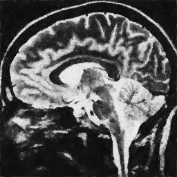
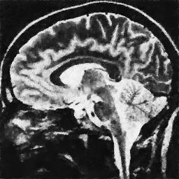
In Figure 1.1 the influence of the choice of a constant λ\lambda in (1.1) is shown, over-regularising the reconstructed image if chosen too small and under-regularising if chosen too large. Moreover, in Figure 1.2 the reconstructed images with constant and spatially-dependent λ\lambda are shown, where λ\lambda has been optimized with the bilevel approach for (1.1) proposed in [9].

Refer to caption
Refer to caption
Figure 1.1. TV denoised images that have been computed as minimizers of (1.1) with different choices for λ∈ℝ+\lambda\in\mathbb{R}^{+}. While choosing λ\lambda too small is over-regularizing the image, choosing it too large is under-regularizing, the question is what the best choice of λ\lambda is and how to compute it.
Refer to caption
Refer to caption
Figure 1.2. TV denoised images, computed as minimizers of (1.1), with a λ\lambda that has been optimised with the bilevel approach in [9]. On the left the optimally computed λ∈ℝ+\lambda\in\mathbb{R}^{+} is constant, on the right the λ\lambda is spatially dependent, computed with the approach proposed and analysed in this paper.

In this article we consider the bilevel optimization approach for (1.1) from [9], with a spatially dependent parameter λ∈H1​(Ω)\lambda\in H^{1}(\Omega) and ϕ⁡(⋅)=(⋅)2\phi(\cdot)=(\cdot)^{2} as presented in Section 2, and investigate first- and second-order optimality conditions for the bilevel problem. In addition to the nonsmooth lower level denoising problems, a positivity constraint on the functional parameter (λ≥0\lambda\geq 0 a.e. in Ω\Omega) has to be imposed to guarantee well-posedness. These elements lead to a nonlinear and nonsmooth first-order optimality system with complementarity relations.

For proving second order sufficient optimality conditions, we improve previous Gâteaux differentiability results of the solution mapping[9] and show that it is actually twice Fréchet differentiable under suitable assumptions. We then define a cone of critical directions and prove the result by utilizing a contradiction argument.

Since the resulting optimality system involves several coupled PDEs (twice the size of the training set), the efficient numerical solution of the problem becomes challenging. We consider a combined Schwarz domain decomposition-semismooth Newton approach, where the domain Ω\Omega is subdivided into overlapping subdomains Ωi\Omega_{i} with optimized transmission conditions (see, e.g., [26, 14, 25]). We apply Schwarz domain decomposition methods directly to the nonlinear optimality system rather than to a linearization of it, and solve, in each subdomain, a reduced nonlinear and nonsmooth optimality system. We propose a semismooth Newton algorithm for the solution of each subdomain system and analyze the local superlinear convergence of the method.

The outline of the paper is as follows. In Section 2 the bilevel optimization problem is stated and analyzed. The analysis involves differentiability properties of the solution operator and the derivation of first and second order optimality conditions. The numerical treatment of the problem is considered in Section 3. The discretization of the problem is described and the domain decomposition and semismooth Newton algorithms are presented. Also the convergence analysis of the semismooth Newton method is carried out. Finally, in Section 4 an exhaustive numerical experimentation is presented. We compare our approach with other spatially-dependent approaches and apply it to problems with large training sets.

2. The bilevel optimization problem in function space

Bilevel optimization encompasses a general class of constrained optimization problems in which the constraint constitutes an optimization problem itself, which is called the lower level problem. The idea of employing bilevel optimization for learning variational image processing approaches arises as minimizing a quality measure for the solution of the variational approach with respect to free parameters in the model. That is, we consider the problem

minλ⁡C⁡(u⁡(λ))\displaystyle\min_{\lambda}~C(u(\lambda))
s.t. ​u​(λ)∈argminu​𝒥​(u,λ),\displaystyle\textrm{s.t. }u(\lambda)\in\mathrm{argmin}_{u}\mathcal{J}(u,\lambda),

where λ\lambda encodes the free parameters and CC is a quality measure for a minimizer of the functional 𝒥\mathcal{J}. If 𝒥\mathcal{J} is the TV denoising functional (1.1) such a free parameter is the regularization parameter λ\lambda. The most standard quality measure used in the bilevel context is the mean of L2L^{2} squared distances of solutions of the variational model to desirable examples that are given in form of a training set. For learning variational image denoising models such a training set consists of noisy images and the corresponding clean/true images. In other contexts the training set will be different, e.g. for image segmentation the training set might consist of the to be segmented image and the true segmentation. Once the parameters in the variational model are learned on the basis of the training set, then the learned model is used for new image data. See [2] for a recent review on bilevel learning in image processing.

In the context of learning image processing approaches, the constraint problem is typically non-smooth — as with TV regularization as in (1.1) — making its robust numerical solution a challenging topic. In particular, the derivation of sharp, analytic optimality conditions usually requires twice-continuous differentiability of the functional in the lower level problem and invertibility of its Hessian. Roughly, this is because the solution of the lower level problem does in general not have an explicit expression and we therefore have to apply the implicit function theorem for being able to insert it in the optimality condition for the upper level problem. A successful strategy for dealing with non-smooth lower level problems, therefore, are targeted, active-inactive set smoothing approaches, such as smoothing the TV with Huber regularization [3, 9, 20]. Another recent proposal for the computational realization of bilevel problems with non-smooth constraints can be found in [24], where the lower level problem is approximated by an iteration of sufficiently smooth update rules. The latter has been derived considering the discrete bilevel problem. In contrast, deriving the optimality conditions for the smoothed-problem in function space as in [3, 9], following the principle of optimize-then-discretize rather than discretize-then-optimize, has the advantage that these conditions can be used to construct resolution independent iterative schemes [17]. This is the approach that we too pursue in this paper.

We consider the bilevel problem for learning the parameter λ\lambda for a smoothed version of the TV denoising model in (1.1). Given a training set (ui†,fi),i=1,…,N,(u_{i}^{\dagger},f_{i}),~i=1,\dots,N, of true and noisy images, respectively, the bilevel optimization problem under consideration reads as follows: Find a minimizer (u1∗,…,uN∗,λ∗)∈[H01​(Ω)]N×H1​(Ω)(u^{*}_{1},\dots,u^{*}_{N},\lambda^{*})\in[H^{1}_{0}(\Omega)]^{N}\times H^{1}(\Omega) of the problem

(2.1a) min(u1,…,uN,λ)∈[H01​(Ω)]N×H1​(Ω)​J​(u1,…,uN,λ):=∑i=1N‖ui−ui†‖L22+β​‖λ‖H1​(Ω)2\displaystyle\underset{(u_{1},\dots,u_{N},\lambda)\in[H^{1}_{0}(\Omega)]^{N}\times H^{1}(\Omega)}{\min}J(u_{1},\dots,u_{N},\lambda):=\sum_{i=1}^{N}\|u_{i}-u_{i}^{\dagger}\|^{2}_{L^{2}}+\beta\|\lambda\|^{2}_{H^{1}(\Omega)}
subject to:
(2.1b) ⟨ei​(ui,λ),v⟩H−1,H01=μ​(D​ui,D​v)L2+(hγ​(D​ui),D​v)L2\displaystyle\langle e_{i}(u_{i},\lambda),v\rangle_{H^{-1},H^{1}_{0}}=\mu\big(Du_{i},Dv\big)_{L^{2}}+\big(h_{\gamma}(Du_{i}),Dv\big)_{L^{2}}
+∫Ωλϕ′(ui,fi)vdx=0 for all v∈H01(Ω),i=1,…,N,\displaystyle\hskip 113.81102pt+\int\limits_{\Omega}{\lambda\phi^{\prime}(u_{i},f_{i})vdx}=0\quad\text{ for all }v\in H^{1}_{0}(\Omega),~i=1,\dots,N,
(2.1c) λ≥0 a.e. in ​Ω,\displaystyle\lambda\geq 0\quad\text{ a.e. in }\Omega,

where NN is the size of the training set of images, 0<μ≪10<\mu\ll 1, ei:H01​(Ω)×H1​(Ω)→H−1​(Ω)e_{i}:H^{1}_{0}(\Omega)\times H^{1}(\Omega)\rightarrow H^{-1}(\Omega), for i=1,…,Ni=1,\dots,N, and

ϕ(ui,fi)=(ui−fi)2,i=1,…,N.\phi(u_{i},f_{i})=(u_{i}-f_{i})^{2},~i=1,\dots,N.

Equations (2.1b) correspond to the necessary and sufficient optimality conditions of a regularized version of the total variation denoising models. In this manner, we replace the lower level minimization problems by an equivalent system of partial differential equations.

The C2C^{2}-regularizing function hγ:ℝn→ℝnh_{\gamma}:\mathbb{R}^{n}\to\mathbb{R}^{n} is given by:

(2.2) hγ​(z)={z|z|ifγ​|z|≥b,z|z|{2​γ−14​γ+γ​|z|2−γ2​(γ​|z|−a)​(γ​|z|−b)+γ32(γ|z|−a)2(γ|z|−b)2}ifa<γ​|z|≤b,γ​zelse,h_{\gamma}(z)=\begin{cases}\frac{z}{|z|}\qquad&\mbox{if}\quad\gamma|z|\geq b,\\ \begin{aligned} \frac{z}{|z|}\bigg\{\frac{2\gamma-1}{4\gamma}&+\frac{\gamma|z|}{2}-\frac{\gamma}{2}\big(\gamma|z|-a\big)\big(\gamma|z|-b\big)\\ &+\frac{\gamma^{3}}{2}\big(\gamma|z|-a\big)^{2}\big(\gamma|z|-b\big)^{2}\bigg\}\end{aligned}\qquad&\mbox{if}\quad a<\gamma|z|\leq b,\\ \gamma z\qquad&\mbox{else,}\end{cases}

where a:=1−12​γa:=1-\frac{1}{2\gamma}, b:=1+12​γb:=1+\frac{1}{2\gamma}, |⋅||\cdot| stands for the euclidean norm and the division has to be understood componentwise. This function locally regularizes the subgradient of the TV-norm around 00. Note that the smoothing applied to the TV denoising problem firstly smoothes the TV with (2.2), and secondly adds a small elliptic regularization term (weighted by μ\mu) to the functional which results in the weak optimality condition in (2.1b). We have outlined the reason for the Huber regularization above. The reason for the addition of the elliptic term μ​‖D​u‖22\mu\|Du\|_{2}^{2} to (1.1) is, that it numerically renders the inversion of the Hessian of the lower level functional more robust and that it places the problem in Hilbert space and therefore opens up a large toolbox for the analysis of the smoothed problem and its approximation properties, see also [8].

The next result involves some properties of hγh_{\gamma}, which will be used throughout the paper.

Lemma 2.1.

The first and second derivative of the function hγ:ℝn→ℝnh_{\gamma}:\mathbb{R}^{n}\to\mathbb{R}^{n} are Lipschitz continuous functions, with Lipschitz constants depending only on γ\gamma.

Proof.

The proof is included in the appendix (Section 5). ∎

In order to simplify the presentation, we focus hereafter on the case N=1N=1. The results are, however, easily extendable to larger training sets, as will be shown in Section 4.

2.1. Differentiability of the solution operator

From [9] we know that for each fixed γ>0\gamma>0, there exists an optimal solution for problem (2.1). Denoting by G:H1​(Ω)→H01​(Ω)G:H^{1}(\Omega)\rightarrow H^{1}_{0}(\Omega) the solution operator G⁡(λ)=uG(\lambda)=u, where uu is solution of equation (2.1b) corresponding to λ∈H1​(Ω)\lambda\in H^{1}(\Omega), it has been shown in [9] that the operator is Gâteaux differentiable. In the next theorem we improve that result and prove that the solution operator is actually Fréchet differentiable.

Theorem 2.1.

Let f∈Lp​(Ω),f\in L^{p}(\Omega), for some p>2p>2, and λ∈Vad:={v∈H1​(Ω):v≥0​ a.e. in ​Ω}\lambda\in V_{\text{ad}}:=\{v\in H^{1}(\Omega):v\geq 0\text{ a.e. in }\Omega\}. Let further B⁡(λ)B(\lambda) be a neighbourhood of λ\lambda. Then, the solution operator

G:B⁡(λ)\displaystyle G:B(\lambda) →H01​(Ω)\displaystyle\rightarrow H^{1}_{0}(\Omega)
λ~\displaystyle\tilde{\lambda} ↦u⁡(λ~),\displaystyle\mapsto u(\tilde{\lambda}),

where u⁡(λ~)u(\tilde{\lambda}) is the solution to (2.1b)(\ref{eq00_1b}) associated to λ~\tilde{\lambda}, is Fréchet differentiable on B⁡(λ)B(\lambda) and its derivative at λ∈Vad\lambda\in V_{\text{ad}}, in direction ξ∈H1​(Ω)\xi\in H^{1}(\Omega), is given by zλξ=G′​(λ)​ξ∈H01​(Ω)z^{\xi}_{\lambda}=G^{\prime}(\lambda)\xi\in H_{0}^{1}(\Omega), which corresponds to the unique solution of the linearized equation:

(2.3) μ​(D​zλξ,D​v)L2+(hγ′​(D​u)​D​zλξ,D​v)L2+2​∫Ωλ​zλξ​v​𝑑x+2​∫Ωξ⁡(u−f)​v​𝑑x=0,∀v∈H01​(Ω).\mu(Dz^{\xi}_{\lambda},Dv\big)_{L^{2}}+\big(h^{\prime}_{\gamma}(Du)Dz^{\xi}_{\lambda},Dv\big)_{L^{2}}+2\int_{\Omega}{\lambda z^{\xi}_{\lambda}v}\,dx+2\int_{\Omega}{\xi(u-f)v}\,dx=0,\forall v\in H^{1}_{0}(\Omega).
Proof.

Along this proof we denote by CC a generic positive constant which may depend on γ\gamma and λ\lambda. Let us also denote by uu and uξu_{\xi} the corresponding solutions to (2.1b) with λ\lambda and λ+ξ\lambda+\xi, respectively. By monotonicity techniques (see [4, Thm. 2.7]), we obtain the existence of a unique solution uξu_{\xi}, for ‖ξ‖H1​(Ω)\|\xi\|_{H^{1}(\Omega)} sufficiently small, and a unique solution zλξ∈H01​(Ω)z^{\xi}_{\lambda}\in H_{0}^{1}(\Omega) to (2.3). Moreover, we get the estimates

(2.4) ‖uξ−u‖H01=O⁡(‖ξ‖H1),‖zλξ‖H01=O⁡(‖ξ‖H1).\|u_{\xi}-u\|_{H^{1}_{0}}=O(\|\xi\|_{H^{1}}),\quad\|z^{\xi}_{\lambda}\|_{H^{1}_{0}}=O(\|\xi\|_{H^{1}}).

By taking the difference between (2.1b), with λ\lambda and λ+ξ\lambda+\xi, and (2.3) we get that

μ​(D⁡(uξ−u−zλξ),D​v)L2\displaystyle\mu\big(D(u_{\xi}-u-z^{\xi}_{\lambda}),Dv\big)_{L^{2}} +(hγ​(D​uξ)−hγ​(D​u)−hγ′​(D​u)​D​zλξ,D​v)L2\displaystyle+\big(h_{\gamma}(Du_{\xi})-h_{\gamma}(Du)-h^{\prime}_{\gamma}(Du)Dz^{\xi}_{\lambda},Dv\big)_{L^{2}}
+2∫Ωλ(uξ−u−zλξ)vdx+2∫Ωξ(uξ−u)vdx=0,∀v∈H01(Ω).\displaystyle+2\int_{\Omega}\lambda(u_{\xi}-u-z^{\xi}_{\lambda})v\,dx+2\int_{\Omega}\xi(u_{\xi}-u)v\,dx=0,\quad\forall v\in H^{1}_{0}(\Omega).

Introducing η:=uξ−u−zλξ\eta:=u_{\xi}-u-z^{\xi}_{\lambda}, we can write the last equation as follows

μ​(D​η,D​v)L2\displaystyle\mu\big(D\eta,Dv\big)_{L^{2}} +(hγ′(Du)Dη,Dv)L2+2∫Ωληvdx=−2∫Ωξ(uξ−u)vdx\displaystyle+\big(h^{\prime}_{\gamma}(Du)D\eta,Dv\big)_{L^{2}}+2\int_{\Omega}\lambda\eta v\,dx=-2\int_{\Omega}\xi(u_{\xi}-u)v\,dx
−(hγ​(D​uξ)−hγ​(D​u)−hγ′​(D​u)​D​(uξ−u),D​v)L2,∀v∈H01​(Ω).\displaystyle-\big(h_{\gamma}(Du_{\xi})-h_{\gamma}(Du)-h^{\prime}_{\gamma}(Du)D(u_{\xi}-u),Dv\big)_{L^{2}},\quad\forall v\in H^{1}_{0}(\Omega).

Taking v=ηv=\eta and using the monotonicity of hγ′​(D​u)h^{\prime}_{\gamma}(Du) and λ≥0\lambda\geq 0 a.e. in Ω\Omega, we get that

‖η‖H012≤|(hγ​(D​uξ)−hγ​(D​u)−hγ′​(D​u)​D​(uξ−u),D​η)L2|+C​‖ξ‖H1​‖uξ−u‖H01​‖η‖H01.\|\eta\|^{2}_{H^{1}_{0}}\leq\bigg|\big(h_{\gamma}(Du_{\xi})-h_{\gamma}(Du)-h^{\prime}_{\gamma}(Du)D(u_{\xi}-u),D\eta\big)_{L^{2}}\bigg|+C\|\xi\|_{H^{1}}\|u_{\xi}-u\|_{H^{1}_{0}}\|\eta\|_{H^{1}_{0}}.

Due to the differentiability of hγh_{\gamma}, we obtain

(2.5) ‖η‖H01≤C⁡(‖uξ−u‖W1,p2+‖ξ‖H1​‖uξ−u‖H01),\|\eta\|_{H^{1}_{0}}\leq C\left(\|u_{\xi}-u\|^{2}_{W^{1,p}}+\|\xi\|_{H^{1}}\|u_{\xi}-u\|_{H^{1}_{0}}\right),

for all p>2p>2 and some constant C>0C>0. Thanks to [16, Thm. 1], there is some p^>2\hat{p}>2 such that

(2.6) ‖uξ−u‖W1,p^=O⁡(‖ξ‖H1).\|u_{\xi}-u\|_{W^{1,\hat{p}}}=O(\|\xi\|_{H^{1}}).

From the latter and estimates (2.4), it then follows that ‖η‖H01=O⁡(‖ξ‖H12)\|\eta\|_{H^{1}_{0}}=O(\|\xi\|^{2}_{H^{1}}). The last relation ensures the Fréchet differentiability of GG and zλξ=G′​(λ)​ξz^{\xi}_{\lambda}=G^{\prime}(\lambda)\xi. ∎

A second-order differentiability result for the solution mapping can also be obtained under certain regularity assumptions on the data. The second derivative is used in the proof of second order sufficient optimality conditions and, in its discretized version, for the convergence analysis of the proposed Newton type algorithms.

Theorem 2.2.

If f∈L∞​(Ω)f\in L^{\infty}(\Omega) and u⁡(λ)∈C1,β​(Ω)u(\lambda)\in C^{1,\beta}(\Omega), for some β∈(0,1)\beta\in(0,1), and there exists p^>4\hat{p}>4 such that

(2.7) ‖uζ−u‖W1,p^≤C​‖ζ‖H1, for any ​ζ∈H1​(Ω),\|u_{\zeta}-u\|_{W^{1,\hat{p}}}\leq C\|\zeta\|_{H^{1}},\text{ for any }\zeta\in H^{1}(\Omega),

then GG is twice Fréchet differentiable and its second derivative, in directions (ξ,ζ)(\xi,\zeta), is given by wλ(ξ,ζ)∈H01​(Ω)w_{\lambda}^{(\xi,\zeta)}\in H_{0}^{1}(\Omega), solution of

(2.8) μ⁡(D​wλ(ξ,ζ),D​v)+(hγ′​(D​u​(λ))​D​wλ(ξ,ζ),D​v)+2​∫Ωλ​wλ(ξ,ζ)​v​𝑑x+(h′′γ(Du(λ))[Dzξλ,Dzλζ],Dv)+2∫Ωζzξλvdx+2∫Ωξzζλvdx=0,∀v∈H01(Ω).\mu\big(Dw_{\lambda}^{(\xi,\zeta)},Dv\big)+\big(h^{\prime}_{\gamma}(Du(\lambda))Dw_{\lambda}^{(\xi,\zeta)},Dv\big)+2\int_{\Omega}\lambda w_{\lambda}^{(\xi,\zeta)}v\,dx\\ +\big(h^{\prime\prime}_{\gamma}(Du(\lambda))[Dz^{\xi}_{\lambda},Dz_{\lambda}^{\zeta}],Dv\big)+2\int_{\Omega}\zeta z^{\xi}_{\lambda}v\,dx+2\int_{\Omega}\xi z^{\zeta}_{\lambda}v\,dx=0,\quad\forall v\in H_{0}^{1}(\Omega).
Remark 2.1.

The Hölder continuity assumption on the gradient of u⁡(λ)u(\lambda) and estimate (2.7) may be proved under some hypothesis on the domain and the data (see [5, Thm. 2.2] and [16, Thm. 1], repectively).

Proof of Theorem 2.2.

If f∈L∞​(Ω)f\in L^{\infty}(\Omega) and u⁡(λ)∈C1,β​(Ω)u(\lambda)\in C^{1,\beta}(\Omega), we obtain from elliptic regularity theory (see, e.g., [29]) that

(2.9) ‖zλξ‖W1,s≤C​‖ξ‖H1, for any ​s>2,\|z^{\xi}_{\lambda}\|_{W^{1,s}}\leq C\|\xi\|_{H^{1}},\text{ for any }s>2,

and

‖η‖W1,r\displaystyle\|\eta\|_{W^{1,r}} ≤C⁡(‖η‖H01+‖ξ⁡(uξ−u)‖Lr+‖hγ​(D​uξ)−hγ​(D​u)−hγ′​(D​u)​D​(uξ−u)‖Lr)\displaystyle\leq C\left(\|\eta\|_{H_{0}^{1}}+\|\xi(u_{\xi}-u)\|_{L^{r}}+\|h_{\gamma}(Du_{\xi})-h_{\gamma}(Du)-h^{\prime}_{\gamma}(Du)D(u_{\xi}-u)\|_{L^{r}}\right)
≤C⁡(‖ξ‖H12+‖ξ‖H1​‖uξ−u‖H01+‖uξ−u‖W1,r2),\displaystyle\leq C\left(\|\xi\|_{H^{1}}^{2}+\|\xi\|_{H^{1}}\|u_{\xi}-u\|_{H_{0}^{1}}+\|u_{\xi}-u\|_{W^{1,r}}^{2}\right),

where C>0C>0 stands for a generic constant and r∈(2,p^)r\in(2,\hat{p}). Thanks to estimates (2.4) and (2.7), we then obtain that

(2.10) ‖η‖W1,r≤Cr​‖ξ‖H1, for ​r∈(2,p^).\|\eta\|_{W^{1,r}}\leq C_{r}\|\xi\|_{H^{1}},\text{ for }r\in(2,\hat{p}).

For ξ,ζ∈H1​(Ω)\xi,\zeta\in H^{1}(\Omega), we denote by wλ(ξ,ζ)w^{(\xi,\zeta)}_{\lambda} the solution of the following equation:

(2.11) μ⁡(D​w,D​v)+(hγ′​(D​u)​D​w,D​v)+2​∫Ωλ​w​v​𝑑x+(h′′γ(Du)[Dzξλ,Dzλζ],Dv)+2∫Ωζzξλvdx+2∫Ωξzζλvdx=0,∀v∈H01(Ω).\mu\big(Dw,Dv\big)+\big(h^{\prime}_{\gamma}(Du)Dw,Dv\big)+2\int_{\Omega}\lambda wv\,dx\\ +\big(h^{\prime\prime}_{\gamma}(Du)[Dz^{\xi}_{\lambda},Dz_{\lambda}^{\zeta}],Dv\big)+2\int_{\Omega}\zeta z^{\xi}_{\lambda}v\,dx+2\int_{\Omega}\xi z^{\zeta}_{\lambda}v\,dx=0,\forall v\in H_{0}^{1}(\Omega).

Existence and uniqueness of wλ(ξ,ζ)w^{(\xi,\zeta)}_{\lambda} follows in a standard manner from the Lax-Milgram theorem.

Let now λζ:=λ+ζ\lambda_{\zeta}:=\lambda+\zeta and let zλζξ:=G′​(λζ)​ξz^{\xi}_{\lambda_{\zeta}}:=G^{\prime}(\lambda_{\zeta})\xi, with uζu_{\zeta} the solution to (2.1b) corresponding to λζ\lambda_{\zeta}. Taking the difference between (2.3) for zλξz^{\xi}_{\lambda} and zλζξz^{\xi}_{\lambda_{\zeta}}, we get

(2.12) μ⁡(D⁡(zλζξ−zλξ),D​v)+(hγ′​(D​u)​D​(zλζξ−zλξ),D​v)+2​∫Ωλ⁡(zλζξ−zλξ)​v​𝑑x+([h′γ(Duζ)−h′γ(Du)]Dzξλζ,Dv)+2∫Ωζzξλζvdx+2∫Ωξ(uζ−u)vdx=0,∀v∈H01(Ω).\mu\big(D(z^{\xi}_{\lambda_{\zeta}}-z^{\xi}_{\lambda}),Dv\big)+\big(h^{\prime}_{\gamma}(Du)D(z^{\xi}_{\lambda_{\zeta}}-z^{\xi}_{\lambda}),Dv\big)+2\int_{\Omega}\lambda(z^{\xi}_{\lambda_{\zeta}}-z^{\xi}_{\lambda})v\,dx\\ +\big(\big[h^{\prime}_{\gamma}(Du_{\zeta})-h^{\prime}_{\gamma}(Du)\big]Dz^{\xi}_{\lambda_{\zeta}},Dv\big)+2\int_{\Omega}\zeta z^{\xi}_{\lambda_{\zeta}}v\,dx+2\int_{\Omega}\xi(u_{\zeta}-u)v\,dx=0,\forall v\in H_{0}^{1}(\Omega).

Testing (2.12) with v=zλζξ−zλξv=z^{\xi}_{\lambda_{\zeta}}-z^{\xi}_{\lambda}, we get

(2.13) ∥zξλζ−zξλ∥2H01≤C{|([h′γ(Duζ)−h′γ(Du)]Dzξλ,D(zξλζ−zξλ))|+|∫Ωζzξλ(zξλζ−zξλ)dx|+|∫Ωξ(uζ−u)(zξλζ−zξλ)dx|}.\|z^{\xi}_{\lambda_{\zeta}}-z^{\xi}_{\lambda}\|^{2}_{H^{1}_{0}}\leq C\bigg\{\bigg|\big(\big[h^{\prime}_{\gamma}(Du_{\zeta})-h^{\prime}_{\gamma}(Du)\big]Dz^{\xi}_{\lambda},D(z^{\xi}_{\lambda_{\zeta}}-z^{\xi}_{\lambda})\big)\bigg|\\ +\bigg|\int_{\Omega}\zeta z^{\xi}_{\lambda}(z^{\xi}_{\lambda_{\zeta}}-z^{\xi}_{\lambda})\,dx\bigg|+\bigg|\int_{\Omega}\xi(u_{\zeta}-u)(z^{\xi}_{\lambda_{\zeta}}-z^{\xi}_{\lambda})\,dx\bigg|\bigg\}.

From the the Lipschitz properties of hγ′​(⋅)h_{\gamma}^{\prime}(\cdot) the last relation yields

‖zλζξ−zλξ‖H01≤C⁡(‖uζ−u‖W1,p^​‖zλξ‖W1,r^+‖ζ‖H1​‖zλξ‖H01+‖ξ‖H1​‖uζ−u‖H01),\|z^{\xi}_{\lambda_{\zeta}}-z^{\xi}_{\lambda}\|_{H^{1}_{0}}\leq C\left(\big\|u_{\zeta}-u\big\|_{W^{1,\hat{p}}}\|z^{\xi}_{\lambda}\|_{W^{1,\hat{r}}}+\|\zeta\|_{H^{1}}\|z^{\xi}_{\lambda}\|_{H^{1}_{0}}+\|\ \xi\|_{H^{1}}\|u_{\zeta}-u\|_{H^{1}_{0}}\right),

with r^\hat{r} such that 1/p^+1/r^≤1/21/\hat{p}+1/\hat{r}\leq 1/2. Considering (2.9) and (2.6), then the following estimate holds

(2.14) ‖zλζξ−zλξ‖H01≤C​‖ζ‖H1​‖ξ‖H1.\|z^{\xi}_{\lambda_{\zeta}}-z^{\xi}_{\lambda}\|_{H^{1}_{0}}\leq C\|\zeta\|_{H^{1}}\|\xi\|_{H^{1}}.

Again, thanks to elliptic regularity theory,

(2.15) ‖zλζξ−zλξ‖W1,q^≤Cp​‖ζ‖H1​‖ξ‖H1, for ​q^=r^​p^r^+p^>2.\|z^{\xi}_{\lambda_{\zeta}}-z^{\xi}_{\lambda}\|_{W^{1,\hat{q}}}\leq C_{p}\|\zeta\|_{H^{1}}\|\xi\|_{H^{1}},\quad\text{ for }\hat{q}=\frac{\hat{r}\hat{p}}{\hat{r}+\hat{p}}>2.

In particular, we may choose r^≥4​p^p^−4\hat{r}\geq\frac{4\hat{p}}{\hat{p}-4}, which yields q^≥4\hat{q}\geq 4.

By setting τ:=zλζξ−zλξ−wλ(ξ,ζ)\tau:=z^{\xi}_{\lambda_{\zeta}}-z^{\xi}_{\lambda}-w^{(\xi,\zeta)}_{\lambda} and subtracting (2.11) from (2.12), we get that

μ⁡(D​τ,D​v)+(hγ′​(D​u)​D​τ,D​v)+2​∫Ωλ​τ​v​dx=−([hγ′​(D​uζ)−hγ′​(D​u)]​D​(zλζξ−zλξ),D​v)−2​∫Ωζ⁡(zλζξ−zλξ)​v​𝑑x−2​∫Ωξ⁡(uζ−u−zλζ)​v​𝑑x−(hγ′​(D​uζ)​D​zλξ−hγ′​(D​u)​D​zλξ−hγ′′​(D​u)​[D​zλξ,D​zλζ],D​v),∀v∈H01​(Ω).\mu\big(D\tau,Dv\big)+\big(h^{\prime}_{\gamma}(Du)D\tau,Dv\big)+2\int_{\Omega}\lambda\tau v\,dx=\\ -\big(\big[h^{\prime}_{\gamma}(Du_{\zeta})-h^{\prime}_{\gamma}(Du)\big]D(z^{\xi}_{\lambda_{\zeta}}-z^{\xi}_{\lambda}),Dv\big)-2\int_{\Omega}\zeta(z^{\xi}_{\lambda_{\zeta}}-z^{\xi}_{\lambda})v\,dx-2\int_{\Omega}\xi(u_{\zeta}-u-z^{\zeta}_{\lambda})v\,dx\\ -\bigg(h^{\prime}_{\gamma}(Du_{\zeta})Dz^{\xi}_{\lambda}-h^{\prime}_{\gamma}(Du)Dz^{\xi}_{\lambda}-h^{\prime\prime}_{\gamma}(Du)[Dz^{\xi}_{\lambda},Dz_{\lambda}^{\zeta}],Dv\bigg),\quad\forall v\in H_{0}^{1}(\Omega).

Testing the last equation with v=τv=\tau and using the ellipticity of the terms on the left hand side, we obtain that

(2.16) ∥τ∥H01≤C{‖[h′γ(Duζ)−h′γ(Du)]D(zξλζ−zξλ)‖L2+‖ζ(zξλζ−zξλ)‖L2++‖ξ(uζ−u−zζλ)‖L2+‖h′γ(Duζ)Dzξλ−h′γ(Du)Dzξλ−h′′γ(Du)[Dzξλ,Dzλζ]‖L2}.\|\tau\|_{H^{1}_{0}}\leq C\bigg\{\left\|\big[h^{\prime}_{\gamma}(Du_{\zeta})-h^{\prime}_{\gamma}(Du)\big]D(z^{\xi}_{\lambda_{\zeta}}-z^{\xi}_{\lambda})\right\|_{L^{2}}+\left\|\zeta(z^{\xi}_{\lambda_{\zeta}}-z^{\xi}_{\lambda})\right\|_{L^{2}}+\\ +\left\|\xi(u_{\zeta}-u-z^{\zeta}_{\lambda})\right\|_{L^{2}}+\left\|h^{\prime}_{\gamma}(Du_{\zeta})Dz^{\xi}_{\lambda}-h^{\prime}_{\gamma}(Du)Dz^{\xi}_{\lambda}-h^{\prime\prime}_{\gamma}(Du)[Dz^{\xi}_{\lambda},Dz_{\lambda}^{\zeta}]\right\|_{L^{2}}\bigg\}.

For the first term on the right hand side, thanks to the Lipschitz continuity of hγ′h_{\gamma}^{\prime} and estimate (2.15), we get that

‖[hγ′​(D​uζ)−hγ′​(D​u)]​D​(zλζξ−zλξ)‖L2\displaystyle\left\|\big[h^{\prime}_{\gamma}(Du_{\zeta})-h^{\prime}_{\gamma}(Du)\big]D(z^{\xi}_{\lambda_{\zeta}}-z^{\xi}_{\lambda})\right\|_{L^{2}} ≤‖hγ′​(D​uζ)−hγ′​(D​u)‖Lp^​‖zλζξ−zλξ‖W1,q^\displaystyle\leq\left\|h^{\prime}_{\gamma}(Du_{\zeta})-h^{\prime}_{\gamma}(Du)\right\|_{L^{\hat{p}}}\left\|z^{\xi}_{\lambda_{\zeta}}-z^{\xi}_{\lambda}\right\|_{W^{1,\hat{q}}}
≤L​‖uζ−u‖W1,p^​‖zλζξ−zλξ‖W1,q^\displaystyle\leq L\|u_{\zeta}-u\|_{W^{1,\hat{p}}}\left\|z^{\xi}_{\lambda_{\zeta}}-z^{\xi}_{\lambda}\right\|_{W^{1,\hat{q}}}
≤C​‖ζ‖H12​‖ξ‖H1.\displaystyle\leq C\|\zeta\|^{2}_{H^{1}}\|\xi\|_{H^{1}}.

Since the solution operator has been proved to be Fréchet differentiable, it follows that ‖uζ−u−zλζ‖H01=o⁡(‖ζ‖H1)\|u_{\zeta}-u-z^{\zeta}_{\lambda}\|_{H^{1}_{0}}=o(\|\zeta\|_{H^{1}}) and, thus,

‖ξ⁡(uζ−u−zλζ)‖L2≤C​‖ξ‖H1​o​(‖ζ‖H1).\left\|\xi(u_{\zeta}-u-z^{\zeta}_{\lambda})\right\|_{L^{2}}\leq C\|\xi\|_{H^{1}}o(\|\zeta\|_{H^{1}}).

From (2.14) it also follows that

‖ζ⁡(zλζξ−zλξ)‖L2≤C​‖ζ‖H12​‖ξ‖H1.\left\|\zeta(z^{\xi}_{\lambda_{\zeta}}-z^{\xi}_{\lambda})\right\|_{L^{2}}\leq C\|\zeta\|^{2}_{H^{1}}\|\xi\|_{H^{1}}.

For the last term on the right hand side of (2.16), we obtain that

‖(hγ′​(D​uζ)−hγ′​(D​u)−hγ′′​(D​u)​D​zλζ)​D​zλξ‖L2≤‖hγ′′​(D​u)​D​(uζ−u−zλζ)‖Lr​‖D​zλξ‖Ls+‖hγ′​(D​uζ)−hγ′​(D​u)−hγ′′​(D​u)​D​(uζ−u)‖Lr​‖D​zλξ‖Ls,\left\|\left(h^{\prime}_{\gamma}(Du_{\zeta})-h^{\prime}_{\gamma}(Du)-h^{\prime\prime}_{\gamma}(Du)Dz^{\zeta}_{\lambda}\right)Dz_{\lambda}^{\xi}\right\|_{L^{2}}\leq\left\|h^{\prime\prime}_{\gamma}(Du)D(u_{\zeta}-u-z_{\lambda}^{\zeta})\right\|_{L^{r}}\|Dz^{\xi}_{\lambda}\|_{L^{s}}\\ +\left\|h^{\prime}_{\gamma}(Du_{\zeta})-h^{\prime}_{\gamma}(Du)-h^{\prime\prime}_{\gamma}(Du)D(u_{\zeta}-u)\right\|_{L^{r}}\|Dz^{\xi}_{\lambda}\|_{L^{s}},

where 1/r+1/s=1/21/r+1/s=1/2 and r∈(2,p^)r\in(2,\hat{p}). Taking into account estimates (2.7), (2.9) and (2.10) we get that

‖(hγ′​(D​uζ)−hγ′​(D​u)−hγ′′​(D​u)​D​zλζ)​D​zλξ‖L2≤C​‖ξ‖H1​(o⁡(‖ζ‖H1)+o⁡(‖uζ−u‖W1,p^)).\left\|\left(h^{\prime}_{\gamma}(Du_{\zeta})-h^{\prime}_{\gamma}(Du)-h^{\prime\prime}_{\gamma}(Du)Dz^{\zeta}_{\lambda}\right)Dz_{\lambda}^{\xi}\right\|_{L^{2}}\leq C\|\xi\|_{H^{1}}\left(o(\|\zeta\|_{H^{1}})+o(\|u_{\zeta}-u\|_{W^{1,\hat{p}}})\right).

Now plugging the last estimates into (2.16) and using (2.7), we get that

‖τ‖H01≤C​‖ξ‖H1​o​(‖ζ‖H1).\|\tau\|_{H^{1}_{0}}\leq C\|\xi\|_{H^{1}}o(\|\zeta\|_{H^{1}}).

The last relation ensures the twice differentiability of GG and we also have that wλ(ξ,ζ)=G′′​(λ)​[ξ,ζ]w^{(\xi,\zeta)}_{\lambda}=G^{\prime\prime}(\lambda)[\xi,\zeta]. ∎

2.2. Optimality conditions

Based on the differentiability properties of the solution operator, a first order optimality system characterizing the optimal weight function is derived next. The solutions to the optimality system are stationary points, which may or may not correspond to local optimal solutions of (2.1). To verify that a stationary point is actually a minimizer, second order sufficient optimality conditions are investigated thereafter.

Theorem 2.3.

Let (u,λ)∈H01​(Ω)×Vad(u,\lambda)\in H^{1}_{0}(\Omega)\times V_{\text{ad}} be an optimal solution for (2.1)(\ref{eq00_1}). Then there exist p∈H01​(Ω)p\in H^{1}_{0}(\Omega) and ϑ∈L2​(Ω)\vartheta\in L^{2}(\Omega) such that the following optimality system holds (in weak sense):

(2.17a) −μ​Δ​u\displaystyle-\mu\Delta u −Div​q+2​λ​(u−f)=0\displaystyle-\mathrm{Div}~q+2\lambda(u-f)=0 in ​Ω,\displaystyle\text{ in }\Omega,
(2.17b) u\displaystyle u =0\displaystyle=0 on ​Γ,\displaystyle\text{ on }\Gamma,
(2.17c) q\displaystyle q =hγ​(D​u)\displaystyle=h_{\gamma}(Du) a.e. in ​Ω,\displaystyle\text{a.e. in }\Omega,
(2.17d) −μ​Δ​p\displaystyle-\mu\Delta p −Div​z+2​(λ​p+u−u†)=0\displaystyle-\mathrm{Div}~z+2(\lambda p+u-u^{\dagger})=0 in ​Ω,\displaystyle\text{ in }\Omega,
(2.17e) p\displaystyle p =0\displaystyle=0 on ​Γ,\displaystyle\text{ on }\Gamma,
(2.17f) z\displaystyle z =hγ′​(D​u)∗​D​p\displaystyle=h^{\prime}_{\gamma}(Du)^{*}Dp a.e. in ​Ω,\displaystyle\text{a.e. in }\Omega,
(2.17g) ϑ\displaystyle\vartheta =−β​Δ​λ+β​λ+(u−f)​p\displaystyle=-\beta\Delta\lambda+\beta\lambda+(u-f)p in ​Ω,\displaystyle\text{ in }\Omega,
(2.17h) ∂λ∂n→\displaystyle\frac{\partial\lambda}{\partial\vec{n}} =0\displaystyle=0 on ​Γ,\displaystyle\text{ on }\Gamma,
(2.17i) λ\displaystyle\lambda ≥0,ϑ≥0,ϑ​λ=0\displaystyle\geq 0,\quad\vartheta\geq 0,\quad\vartheta\,\lambda=0 a.e. in ​Ω.\displaystyle\text{a.e. in }\Omega.
Proof.

Since the solution operator is differentiable, it follows, using the reduced cost functional

(2.18) 𝒥⁡(λ)=‖u⁡(λ)−u†‖L22+β​‖λ‖H1​(Ω)2,\mathcal{J}(\lambda)=\|u(\lambda)-u^{\dagger}\|^{2}_{L^{2}}+\beta\|\lambda\|^{2}_{H^{1}(\Omega)},

that

(2.19) 𝒥′​(λ)​(ξ−λ)=(u⁡(λ)−u†,u′​(λ)​(ξ−λ))+β​(λ,ξ−λ)H1≥0,∀ξ∈Vad.\mathcal{J}^{\prime}(\lambda)(\xi-\lambda)=(u(\lambda)-u^{\dagger},u^{\prime}(\lambda)(\xi-\lambda))+\beta(\lambda,\xi-\lambda)_{H^{1}}\geq 0,\qquad\forall\xi\in V_{\text{ad}}.

Introducing p∈H01​(Ω)p\in H_{0}^{1}(\Omega) as the unique weak solution of the adjoint equations (2.17d)-(2.17f) and using the linearised equation (2.3), we obtain that

2​(u−u†,u′)\displaystyle 2(u-u^{\dagger},u^{\prime}) =−μ⁡(D​p,D​u′)−∫Ωhγ′​(D​u)∗​D​p⋅D​u′​𝑑x−2​∫Ωλ​u′​p​𝑑x\displaystyle=-\mu(Dp,Du^{\prime})-\int_{\Omega}h_{\gamma}^{\prime}(Du)^{*}Dp\cdot Du^{\prime}\,dx-2\int_{\Omega}\lambda u^{\prime}p\,dx
=2​∫Ωp⁡(u−f)​(ξ−λ)​𝑑x,\displaystyle=2\int_{\Omega}p(u-f)(\xi-\lambda)\,dx,

where we used the notation u′:=u′​(λ)​(ξ−λ)u^{\prime}:=u^{\prime}(\lambda)(\xi-\lambda). Replacing the last term in (2.18), we get that

(2.20) β​(λ,ξ−λ)H1+∫Ωp⁡(u−f)​(ξ−λ)​𝑑x≥0,∀ξ∈Vad.\beta(\lambda,\xi-\lambda)_{H^{1}}+\int_{\Omega}p(u-f)(\xi-\lambda)\,dx\geq 0,\quad\forall\xi\in V_{\text{ad}}.

Inequality (2.20) corresponds to an obstacle type problem with unilateral bounds. Thanks to regularity results for this type of problems (see [29, Thm.5.2,  p.294]), it follows that λ∈H2​(Ω)\lambda\in H^{2}(\Omega) (if f∈Lp​(Ω)f\in L^{p}(\Omega) for some p>2p>2) and, therefore, we may define

ϑ:=−β​Δ​λ+β​λ+(u−f)​p∈L2​(Ω).\vartheta:=-\beta\Delta\lambda+\beta\lambda+(u-f)p\in L^{2}(\Omega).

Integrating by parts in (2.20) we then obtain that (ϑ,ξ−λ)L2≥0\big(\vartheta,\xi-\lambda\big)_{L^{2}}\geq 0. From the latter and the sign of λ\lambda, we finally get that

(2.21) λ≥0,ϑ≥0,ϑλ\displaystyle\lambda\geq 0,\quad\vartheta\geq 0,\quad\vartheta~\lambda =0a.e.Ω.\displaystyle=0\quad a.e.\quad\Omega.

∎

Remark 2.2.

If u†∈L∞​(Ω)u^{\dagger}\in L^{\infty}(\Omega) and u⁡(λ)∈C1,β​(Ω)u(\lambda)\in C^{1,\beta}(\Omega), it follows from elliptic regularity theory (see, e.g., [29]) that the adjoint state has the extra regularity p∈W1,q​(Ω)p\in W^{1,q}(\Omega), for all q∈(2,+∞)q\in(2,+\infty), and

(2.22) ‖p‖W1,q≤Cq​‖u−u†‖L∞.\|p\|_{W^{1,q}}\leq C_{q}\|u-u^{\dagger}\|_{L^{\infty}}.

The complementarity condition (2.21) can also be reformulated as the following nonsmooth equation:

ϑ=max⁡(0,ϑ−α​λ), for any ​α>0,\vartheta=\max(0,\vartheta-\alpha\lambda),\text{ for any }\alpha>0,

where the max\max operation has to be understood in an almost everywhere sense. By choosing α=β\alpha=\beta and using (2.17g) one gets

(2.23) −β​Δ​λ+β​λ+(u−f)​p−max⁡(0,−β​Δ​λ+(u−f)​p)=0.-\beta\Delta\lambda+\beta\lambda+(u-f)p-\max(0,-\beta\Delta\lambda+(u-f)p)=0.

Altogether, we obtain the following system for y=(u,q,p,z,λ)y=(u,q,p,z,\lambda)

(2.24) F⁡(y)=(−μ​Δ​u−Div​q+2​λ​(u−f)hγ​(D​u)−q−μ​Δ​p−Div​z+2​λ​p+2​(u−u†)hγ′​(D​u)∗​D​p−z−β​Δ​λ+β​λ+(u−f)​p−max⁡(0,−β​Δ​λ+(u−f)​p))=0,F(y)=\left(\begin{array}[]{c}-\mu\Delta u-\mathrm{Div}\hskip 2.5ptq+2\lambda(u-f)\\ h_{\gamma}(Du)-q\\ -\mu\Delta p-\mathrm{Div}\hskip 2.5ptz+2\lambda p+2(u-u^{\dagger})\\ h^{\prime}_{\gamma}(Du)^{*}Dp-z\\ -\beta\Delta\lambda+\beta\lambda+(u-f)p-\max\big(0,-\beta\Delta\lambda+(u-f)p\big)\end{array}\right)=0,

where F:V→WF:V\to W with V:=H01​(Ω)×L2​(Ω)×H01​(Ω)×L2​(Ω)×H1​(Ω)V:=H^{1}_{0}(\Omega)\times L^{2}(\Omega)\times H^{1}_{0}(\Omega)\times L^{2}(\Omega)\times H^{1}(\Omega) and W:=H−1​(Ω)×L2​(Ω)×H−1​(Ω)×L2​(Ω)×H1​(Ω)′W:=H^{-1}(\Omega)\times L^{2}(\Omega)\times H^{-1}(\Omega)\times L^{2}(\Omega)\times H^{1}(\Omega)^{\prime}. The last equation in (2.24) is complemented with homogeneous Neumann boundary condition for λ\lambda.

As mentioned previously, sufficient optimality conditions are important in order to verify that a given stationary point is indeed a minimizer of the original optimization problem. Thanks to the differentiability properties of the solution mapping (see Theorem 2.2), we can derive a second-order sufficient optimality condition. To state it, let us start by computing the second derivatives of J⁡(u,λ)J(u,\lambda) and the state equation operator e⁡(u,λ)e(u,\lambda) defined in (2.1b). For (u,λ)∈H01​(Ω)×H1​(Ω)(u,\lambda)\in H_{0}^{1}(\Omega)\times H^{1}(\Omega) and for all w,η∈H01​(Ω),l∈H1​(Ω)w,\eta\in H^{1}_{0}(\Omega),l\in H^{1}(\Omega), we have:

(2.25a) eλ​λ​(u,λ)=0\displaystyle e_{\lambda\lambda}(u,\lambda)=0
(2.25b) ⟨eu​λ​(u,λ)​[w,l],v⟩H−1,H01=2​∫Ωw​l​v​𝑑x∀v∈H01​(Ω)\displaystyle\langle e_{u\lambda}(u,\lambda)[w,l],v\rangle_{H^{-1},H^{1}_{0}}=2\int_{\Omega}wlv\,dx\quad\forall v\in H^{1}_{0}(\Omega)
(2.25c) ⟨eu​u​(u,λ)​[w,η],v⟩H−1,H01=∫Ωh′′​(D​u)​[D​w,D​η]⋅D​v​𝑑x,∀v∈H01​(Ω).\displaystyle\langle e_{uu}(u,\lambda)[w,\eta],v\rangle_{H^{-1},H^{1}_{0}}=\int_{\Omega}h^{\prime\prime}(Du)[Dw,D\eta]\cdot Dv\,dx,\quad\forall v\in H^{1}_{0}(\Omega).

Note that for any fixed λ∈H1​(Ω)\lambda\in H^{1}(\Omega) and u∈H01​(Ω)u\in H^{1}_{0}(\Omega), we also get

(2.26) ⟨eu​(u,λ)​w,v⟩H−1,H01=μ​(D​w,D​v)L2+(hγ′​(D​u)​D​w,D​v)L2+2​∫Ωλ​w​v​𝑑x,\langle e_{u}(u,\lambda)w,v\rangle_{H^{-1},H^{1}_{0}}=\mu\big(Dw,Dv\big)_{L^{2}}+\big(h^{\prime}_{\gamma}(Du)Dw,Dv\big)_{L^{2}}+2\int_{\Omega}{\lambda wv}\,dx,

for all v∈H01​(Ω)v\in H^{1}_{0}(\Omega). Now let a:=1−12​γa:=1-\frac{1}{2\gamma} and b:=1+12​γb:=1+\frac{1}{2\gamma}, and let us introduce the sets

(2.27) 𝒜γ​(u)\displaystyle\mathcal{A}^{\gamma}(u) :={∈Ω:γ​|D​u​(x)|≥b},\displaystyle:=\big\{\in\Omega:\gamma|Du(x)|\geq b\big\},
𝒮γ​(u)\displaystyle\mathcal{S}^{\gamma}(u) :={x∈Ω:a<γ​|D​u​(x)|<b},\displaystyle:=\big\{x\in\Omega:a<\gamma|Du(x)|<b\big\},
ℐγ​(u)\displaystyle\mathcal{I}^{\gamma}(u) :={x∈Ω:γ​|D​u​(x)|≤a},\displaystyle:=\big\{x\in\Omega:\gamma|Du(x)|\leq a\big\},

and t1​(u):=γ2​(γ​|D​u|−a)=γ2​(γ​|D​u|−1+12​γ)t_{1}(u):=\frac{\gamma}{2}\big(\gamma|Du|-a\big)=\frac{\gamma}{2}\big(\gamma|Du|-1+\frac{1}{2\gamma}\big); t2​(u)=γ​|D​u|−1−32​γt_{2}(u)=\gamma|Du|-1-\frac{3}{2\gamma}. For all z∈H01​(Ω)z\in H^{1}_{0}(\Omega), we get the following expressions for the derivatives of hγh_{\gamma}:

(2.28) hγ′​(D​u)​D​z\displaystyle h^{\prime}_{\gamma}(Du)Dz =χ𝒜γ​(u)​{D​z|D​u|−⟨D​u,D​z⟩|D​u|3​D​u}+γ​χℐγ​(u)​(D​z)\displaystyle=\chi_{\mathcal{A}^{\gamma}(u)}\bigg\{\dfrac{Dz}{|Du|}-\dfrac{\langle Du,Dz\rangle}{|Du|^{3}}Du\bigg\}+\gamma\chi_{\mathcal{I}^{\gamma}(u)}\big(Dz\big)
+χ𝒮γ​(u){γ2Dz+γ2(γ|Du|−1)[2γ2t1(u)t2(u)−1]⟨D​u,D​z⟩|D​u|2Du\displaystyle+\chi_{\mathcal{S}^{\gamma}(u)}\bigg\{\frac{\gamma}{2}Dz+\gamma^{2}\big(\gamma|Du|-1\big)\bigg[2\gamma^{2}t_{1}(u)t_{2}(u)-1\bigg]\frac{\langle Du,Dz\rangle}{|Du|^{2}}Du
+[2​γ−14​γ−γ​t1​(u)​t2​(u)2+γ3​t12​(u)​t22​(u)2](D​z|D​u|−⟨D​u,D​z⟩|D​u|3Du)}\displaystyle+\bigg[\dfrac{2\gamma-1}{4\gamma}-\dfrac{\gamma t_{1}(u)t_{2}(u)}{2}+\dfrac{\gamma^{3}t^{2}_{1}(u)t^{2}_{2}(u)}{2}\bigg]\bigg(\frac{Dz}{|Du|}-\frac{\langle Du,Dz\rangle}{|Du|^{3}}Du\bigg)\bigg\}

and

(2.29) hγ′′​(D​u)​[D​p,D​z]\displaystyle h^{\prime\prime}_{\gamma}(Du)[Dp,Dz] =χ𝒜γ​(u)​Φ​(D​u,D​p)​D​z\displaystyle=\chi_{\mathcal{A}^{\gamma}(u)}\Phi(Du,Dp)Dz
+χ𝒮γ​(u)\displaystyle+\chi_{\mathcal{S}^{\gamma}(u)} {[γ2t1(u)t2(u)(4γ3|Du|(γ|Du|−1)−γ2t1(u)t2(u)+1)\displaystyle\bigg\{\bigg[\frac{\gamma}{2}t_{1}(u)t_{2}(u)\bigg(4\gamma^{3}|Du|\big(\gamma|Du|-1\big)-\gamma^{2}t_{1}(u)t_{2}(u)+1\bigg)
−(γ3|Du|2−γ2|Du|+12−14​γ)]Φ(Du,Dp)Dz\displaystyle-\bigg(\gamma^{3}|Du|^{2}-\gamma^{2}|Du|+\frac{1}{2}-\frac{1}{4\gamma}\bigg)\bigg]\Phi(Du,Dp)Dz
+6γ5t1(u)t2(u)⟨D​u,D​p⟩​(D​u​D​uT)|D​u|3Dz},\displaystyle+6\gamma^{5}t_{1}(u)t_{2}(u)\frac{\langle Du,Dp\rangle(DuDu^{T})}{|Du|^{3}}Dz\bigg\},

with the operator

Φ⁡(D​u,D​p):=3​⟨D​u,D​p⟩​(D​u​D​uT)|D​u|5−(D​p​D​uT)|D​u|3−(D​u​D​pT)|D​u|3−⟨D​u,D​p⟩|D​u|3.\Phi(Du,Dp):=\dfrac{3\langle Du,Dp\rangle(DuDu^{T})}{|Du|^{5}}-\dfrac{(DpDu^{T})}{|Du|^{3}}-\dfrac{(DuDp^{T})}{|Du|^{3}}-\dfrac{\langle Du,Dp\rangle}{|Du|^{3}}.

We also define the cone of critical directions by

(2.30) 𝒦⁡(λ∗)={l∈H1​(Ω):l⁡(x)​{=0ifϑ(x)≠0≥0ifϑ(x)=0andλ∗(x)=0}.\mathcal{K}(\lambda^{*})=\left\{l\in H^{1}(\Omega):l(x)\begin{cases}=0\quad\mbox{if}\quad\vartheta(x)\not=0\\ \geq 0\quad\mbox{if}\quad\vartheta(x)=0\quad\mbox{and}\quad\lambda^{*}(x)=0\end{cases}\right\}.

Now let us state the second order optimality condition for problem (2.1). The proof goes along the lines of [7, 6]. However, since in our case the control enters in a bilinear way and the PDE has a quasilinear structure, the proof has to be modified accordingly.

Theorem 2.4.

Under the same hypotheses of Theorem 2.2, let (u∗,λ∗,p∗)(u^{*},\lambda^{*},p^{*}) be a solution of the optimality system (2.17) and suppose that there exists ρ>0\rho>0 such that

(2.31) 2​‖w‖L22+2​β​‖l‖H12+∫Ωh′′​(D​u∗)​[D​w]2⋅D​p∗​𝑑x+4​∫Ωw​l​p∗​𝑑x≥ρ​‖l‖H12,2\|w\|^{2}_{L^{2}}+2\beta\|l\|^{2}_{H^{1}}+\int_{\Omega}h^{\prime\prime}(Du^{*})[Dw]^{2}\cdot Dp^{*}\,dx+4\int_{\Omega}wlp^{*}\,dx\geq\rho\|l\|^{2}_{H^{1}},

for every pair (w,l)∈H01​(Ω)×𝒦⁡(λ∗)(w,l)\in H^{1}_{0}(\Omega)\times\mathcal{K}(\lambda^{*}), (w,l)≠(0,0)(w,l)\not=(0,0) which satisfies the linearized equation:

(2.32) μ​(D​w,D​v)L2+(hγ′​(D​u∗)​D​w,D​v)L2+2​∫Ωl⁡(u∗−f)​v​𝑑x+2​∫Ωλ∗​w​v​𝑑x=0,∀v∈V.\mu\big(Dw,Dv\big)_{L^{2}}+\big(h^{\prime}_{\gamma}(Du^{*})Dw,Dv\big)_{L^{2}}+2\int_{\Omega}l(u^{*}-f)v\,dx+2\int_{\Omega}\lambda^{*}wv\,dx=0,\forall v\in V.

Then there exist σ>0\sigma>0 and τ>0\tau>0 such that

(2.33) J⁡(u∗,λ∗)+τ​‖λ−λ∗‖H12≤J⁡(u,λ),J(u^{*},\lambda^{*})+\tau\|\lambda-\lambda^{*}\|^{2}_{H^{1}}\leq J(u,\lambda),

for every feasible pair (u,λ)(u,\lambda) such that u=G⁡(λ)u=G(\lambda) and ‖λ−λ∗‖H1≤σ\|\lambda-\lambda^{*}\|_{H^{1}}\leq\sigma.

Proof.

Suppose that λ∗\lambda^{*} does not satisfy the growth condition (2.33). Then there exists a feasible sequence {λk}k⊂H1​(Ω)\{\lambda_{k}\}_{k}\subset H^{1}(\Omega) such that

(2.34) ‖λk−λ∗‖H1\displaystyle\|\lambda_{k}-\lambda^{*}\|_{H^{1}} <1k2and\displaystyle<\frac{1}{k^{2}}\quad\mbox{and}
(2.35) J⁡(u∗,λ∗)+1k​‖λ−λ∗‖H12\displaystyle J(u^{*},\lambda^{*})+\frac{1}{k}\|\lambda-\lambda^{*}\|^{2}_{H^{1}} >J(uk,λk)=ℒ(uk,λk,p∗)∀k,\displaystyle>J(u_{k},\lambda_{k})=\mathcal{L}(u_{k},\lambda_{k},p^{*})\quad\forall k,

where uk=G⁡(λk)u_{k}=G(\lambda_{k}) and ℒ⁡(u,λ,p):=⟨e⁡(u,λ),p⟩H−1,H01+J⁡(u,λ)\mathcal{L}(u,\lambda,p):=\langle e(u,\lambda),p\rangle_{H^{-1},H_{0}^{1}}+J(u,\lambda). From (2.7) we then get that uk→u∗u_{k}\to u^{*} strongly in W1,p^,W^{1,\hat{p}}, with p^>4\hat{p}>4. By setting ρk=‖λk−λ∗‖H1\rho_{k}=\|\lambda_{k}-\lambda^{*}\|_{H^{1}} and ζk=1ρk​(λk−λ∗)\zeta_{k}=\frac{1}{\rho_{k}}(\lambda_{k}-\lambda^{*}) it follows that ‖ζk‖H1=1\|\zeta_{k}\|_{H^{1}}=1 and therefore we may extract a subsequence, denoted the same, which converges to ζ\zeta weakly in H1​(Ω)H^{1}(\Omega).

Step 1. By the mean value theorem we have

ℒ⁡(uk,λk,p∗)+ℒu​(νk,λk,p∗)​(u∗−uk)\displaystyle\mathcal{L}(u_{k},\lambda_{k},p^{*})+\mathcal{L}_{u}(\nu_{k},\lambda_{k},p^{*})(u^{*}-u_{k}) =ℒ⁡(u∗,λk,p∗)\displaystyle=\mathcal{L}(u^{*},\lambda_{k},p^{*})
=ℒ⁡(u∗,λ∗,p∗)+ρk​ℒλ​(u∗,ξk,p∗)​ζk\displaystyle=\mathcal{L}(u^{*},\lambda^{*},p^{*})+\rho_{k}\mathcal{L}_{\lambda}(u^{*},\xi_{k},p^{*})\zeta_{k}

where νk\nu_{k}, ξk\xi_{k} are points between u∗u^{*} and uku_{k}, λ∗\lambda^{*} and λk\lambda_{k}, respectively. From (2.35) and J⁡(u∗,λ∗)=ℒ⁡(u∗,λ∗,p∗)J(u^{*},\lambda^{*})=\mathcal{L}(u^{*},\lambda^{*},p^{*}) it follows that

(2.36) ℒλ​(u∗,ξk,p∗)​ζk<1k​‖λk−λ∗‖H1+1ρk​ℒu​(νk,λk,p∗)​(u∗−uk).\mathcal{L}_{\lambda}(u^{*},\xi_{k},p^{*})\zeta_{k}<\frac{1}{k}\|\lambda_{k}-\lambda^{*}\|_{H^{1}}+\frac{1}{\rho_{k}}\mathcal{L}_{u}(\nu_{k},\lambda_{k},p^{*})(u^{*}-u_{k}).

By using again the mean value theorem for the last term on the first variable, we obtain

ℒu​(νk,λk,p∗)​(u∗−uk)=\displaystyle\mathcal{L}_{u}(\nu_{k},\lambda_{k},p^{*})(u^{*}-u_{k})= Ju​(νk)​(u∗−uk)+⟨p∗,eu​(νk,λk)​(u∗−uk)⟩H01,H−1\displaystyle J_{u}(\nu_{k})(u^{*}-u_{k})+\langle p^{*},e_{u}(\nu_{k},\lambda_{k})(u^{*}-u_{k})\rangle_{H^{1}_{0},H^{-1}}
=\displaystyle= Ju​(νk)​(u∗−uk)+⟨p∗,eu​(u∗,λk)​(u∗−uk)⟩H01,H−1\displaystyle J_{u}(\nu_{k})(u^{*}-u_{k})+\langle p^{*},e_{u}(u^{*},\lambda_{k})(u^{*}-u_{k})\rangle_{H^{1}_{0},H^{-1}}
+⟨p∗,eu​u​(u∗,λk)​(νk−u∗)​(u∗−uk)⟩H01,H−1\displaystyle+\langle p^{*},e_{uu}(u^{*},\lambda_{k})(\nu_{k}-u^{*})(u^{*}-u_{k})\rangle_{H^{1}_{0},H^{-1}}
+⟨p∗,(eu​u​(ηk,λk)−eu​u​(u∗,λk))​(νk−u∗)​(u∗−uk)⟩H01,H−1,\displaystyle+\big\langle p^{*},\big(e_{uu}(\eta_{k},\lambda_{k})-e_{uu}(u^{*},\lambda_{k})\big)(\nu_{k}-u^{*})(u^{*}-u_{k})\big\rangle_{H^{1}_{0},H^{-1}},

where ηk=u∗+t⁡(νk−u∗)\eta_{k}=u^{*}+t(\nu_{k}-u^{*}), for some t∈[0,1]t\in[0,1]. From (2.26) and the optimality system (2.17) it follows that

⟨p∗,eu(u∗,λk)(u∗−\displaystyle\langle p^{*},e_{u}(u^{*},\lambda_{k})(u^{*}- uk)⟩H01,H−1\displaystyle u_{k})\rangle_{H^{1}_{0},H^{-1}}
=\displaystyle= ⟨p∗,eu​(u∗,λ∗)​(u∗−uk)⟩H01,H−1+2​∫Ω(λk−λ∗)​(u∗−uk)​p∗​𝑑x\displaystyle\langle p^{*},e_{u}(u^{*},\lambda^{*})(u^{*}-u_{k})\rangle_{H^{1}_{0},H^{-1}}+2\int_{\Omega}(\lambda_{k}-\lambda^{*})(u^{*}-u_{k})p^{*}\,dx
=\displaystyle= −Ju​(u∗)​(u∗−uk)+2​∫Ω(λk−λ∗)​(u∗−uk)​p∗​𝑑x.\displaystyle-J_{u}(u^{*})(u^{*}-u_{k})+2\int_{\Omega}(\lambda_{k}-\lambda^{*})(u^{*}-u_{k})p^{*}\,dx.

Hence, from the Lipschitz continuity and the boundedness of hγ′′h_{\gamma}^{\prime\prime}, and the extra regularity of pp (see Remark 2.2), we get

|ℒu​(νk,λk,p∗)​(u∗−uk)|≤\displaystyle\big|\mathcal{L}_{u}(\nu_{k},\lambda_{k},p^{*})(u^{*}-u_{k})\big|\leq ‖Ju​(νk)−Ju​(u∗)‖H−1​‖u∗−uk‖H01\displaystyle\|J_{u}(\nu_{k})-J_{u}(u^{*})\|_{H^{-1}}\|u^{*}-u_{k}\|_{H^{1}_{0}}
+2​‖λk−λ∗‖L3​‖u∗−uk‖L3​‖p∗‖L3\displaystyle+2\|\lambda_{k}-\lambda^{*}\|_{L^{3}}\|u^{*}-u_{k}\|_{L^{3}}\|p^{*}\|_{L^{3}}
+L1γ​‖p∗‖H01​‖νk−u∗‖W1,p^​‖u∗−uk‖W1,p^\displaystyle+L^{\gamma}_{1}\|p^{*}\|_{H^{1}_{0}}\|\nu_{k}-u^{*}\|_{W^{1,\hat{p}}}\|u^{*}-u_{k}\|_{W^{1,\hat{p}}}
+L2γ​‖p∗‖W1,4​‖νk−u∗‖W1,p^2​‖u∗−uk‖W1,p^.\displaystyle+L^{\gamma}_{2}\|p^{*}\|_{W^{1,4}}\|\nu_{k}-u^{*}\|^{2}_{W^{1,\hat{p}}}\|u^{*}-u_{k}\|_{W^{1,\hat{p}}}.

Due to the quadratic cost and the convergence ζk⇀ζ\zeta_{k}\rightharpoonup\zeta, ξk→λ∗\xi_{k}\rightarrow\lambda^{*} in H1​(Ω)H^{1}(\Omega) and uk→u∗u_{k}\rightarrow u^{*} in W1,4​(Ω)W^{1,4}(\Omega), from (2.36) it follows that

ℒλ​(u∗,λ∗,p∗)​ζ=limk→∞​ℒλ​(u∗,ξk,p∗)​ζk≤0.\mathcal{L}_{\lambda}(u^{*},\lambda^{*},p^{*})\zeta=\underset{k\rightarrow\infty}{\lim}\mathcal{L}_{\lambda}(u^{*},\xi_{k},p^{*})\zeta_{k}\leq 0.

On the other hand, since λk​(x)≥0\lambda_{k}(x)\geq 0 a.e in Ω\Omega, it follows that

(2.37) ℒλ​(u∗,λ∗,p∗)​ζk=ρk​ℒλ​(u∗,λ∗,p∗)​(λk−λ∗)≥0.\mathcal{L}_{\lambda}(u^{*},\lambda^{*},p^{*})\zeta_{k}=\rho_{k}\mathcal{L}_{\lambda}(u^{*},\lambda^{*},p^{*})(\lambda_{k}-\lambda^{*})\geq 0.

Since ζk⇀ζ\zeta_{k}\rightharpoonup\zeta one gets ℒλ​(u∗,λ∗,p∗)​ζ=limk→∞​ℒλ​(u∗,λ∗,p∗)​ζk≥0\mathcal{L}_{\lambda}(u^{*},\lambda^{*},p^{*})\zeta=\underset{k\rightarrow\infty}{\lim}\mathcal{L}_{\lambda}(u^{*},\lambda^{*},p^{*})\zeta_{k}\geq 0. Altogether we obtain that ℒλ​(u∗,λ∗,p∗)​ζ=0\mathcal{L}_{\lambda}(u^{*},\lambda^{*},p^{*})\zeta=0.

Step 2. Now we will show that ζ∈𝒦⁡(λ∗)\zeta\in\mathcal{K}(\lambda^{*}). The set

{v∈H1(Ω):v(x)≥0ifϑ(x)=0andλ∗(x)=0}\left\{v\in H^{1}(\Omega):v(x)\geq 0\quad\mbox{if}\quad\vartheta(x)=0\quad\mbox{and}\quad\lambda^{*}(x)=0\right\}

is convex and closed, hence it is weakly sequentially closed. Since λk\lambda_{k} is feasible, then for each kk, ζk\zeta_{k} belongs to this set and, consequently, ζ\zeta also does. From (2.17i) it follows that ϑ⁡(x)​ζ​(x)≥0\vartheta(x)\zeta(x)\geq 0 a.e in Ω\Omega, which implies

0=ℒλ​(u∗,λ∗,p∗)​ζ=β​(λ∗,ζ)H1+∫Ω(u∗−f)​p∗​ζ=∫Ωϑ​ζ​𝑑x=∫Ω|ϑ​ζ|​𝑑x.0=\mathcal{L}_{\lambda}(u^{*},\lambda^{*},p^{*})\zeta=\beta\big(\lambda^{*},\zeta\big)_{H^{1}}+\int\limits_{\Omega}{(u^{*}-f)p^{*}\zeta}=\int_{\Omega}\vartheta\zeta\,dx=\int_{\Omega}|\vartheta\zeta|\,dx.

It follows that ζ⁡(x)=0\zeta(x)=0 if ϑ⁡(x)≠0\vartheta(x)\not=0 and therefore ζ∈𝒦⁡(λ∗)\zeta\in\mathcal{K}(\lambda^{*}).

Step 3 (ζ=0\zeta=0). Using a Taylor expansion of the Lagrangian ℒ\mathcal{L} at (u∗,λ∗,p∗)(u^{*},\lambda^{*},p^{*}) we have

(2.38) ℒ⁡(uk,λk,p∗)=\displaystyle\mathcal{L}(u_{k},\lambda_{k},p^{*})= ℒ⁡(u∗,λ∗,p∗)+ρk​ℒλ​(u∗,λ∗,p∗)​ζk+ρk22​ℒλ​λ​(u∗,λ∗,p∗)​ζk2\displaystyle\mathcal{L}(u^{*},\lambda^{*},p^{*})+\rho_{k}\mathcal{L}_{\lambda}(u^{*},\lambda^{*},p^{*})\zeta_{k}+\frac{\rho_{k}^{2}}{2}\mathcal{L}_{\lambda\lambda}(u^{*},\lambda^{*},p^{*})\zeta_{k}^{2}
+ρk​ℒu​λ​(u∗,λ∗,p∗)​(uk−u∗)​ζk+12​ℒu​u​(νk,λ∗,p∗)​(uk−u∗)2,\displaystyle+\rho_{k}\mathcal{L}_{u\lambda}(u^{*},\lambda^{*},p^{*})(u_{k}-u^{*})\zeta_{k}+\frac{1}{2}\mathcal{L}_{uu}(\nu_{k},\lambda^{*},p^{*})(u_{k}-u^{*})^{2},

where νk\nu_{k} is an intermediate point between uku_{k} and u∗u^{*}. Therefore, thanks to the bilinear control structure,

(2.39) ρk​ℒλ​(u∗,λ∗,p∗)​ζk\displaystyle\rho_{k}\mathcal{L}_{\lambda}(u^{*},\lambda^{*},p^{*})\zeta_{k} +ρk22​ℒλ​λ​(u∗,λ∗,p∗)​ζk2+ρk​ℒu​λ​(u∗,λ∗,p∗)​(uk−u∗)​ζk\displaystyle+\frac{\rho_{k}^{2}}{2}\mathcal{L}_{\lambda\lambda}(u^{*},\lambda^{*},p^{*})\zeta_{k}^{2}+\rho_{k}\mathcal{L}_{u\lambda}(u^{*},\lambda^{*},p^{*})(u_{k}-u^{*})\zeta_{k}
+ρk22​ℒu​u​(u∗,λ∗,p∗)​(uk−u∗ρk)2\displaystyle+\frac{\rho_{k}^{2}}{2}\mathcal{L}_{uu}(u^{*},\lambda^{*},p^{*})\bigg(\frac{u_{k}-u^{*}}{\rho_{k}}\bigg)^{2}
=ℒ⁡(uk,λk,p∗)\displaystyle=\mathcal{L}(u_{k},\lambda_{k},p^{*}) −ℒ⁡(u∗,λ∗,p∗)\displaystyle-\mathcal{L}(u^{*},\lambda^{*},p^{*})
+ρk22​[ℒu​u​(u∗,λ∗,p∗)−ℒu​u​(νk,λ∗,p∗)]​(uk−u∗ρk)2.\displaystyle+\frac{\rho_{k}^{2}}{2}\bigg[\mathcal{L}_{uu}(u^{*},\lambda^{*},p^{*})-\mathcal{L}_{uu}(\nu_{k},\lambda^{*},p^{*})\bigg]\bigg(\frac{u_{k}-u^{*}}{\rho_{k}}\bigg)^{2}.

Moreover, from (2.35) it follows that

(2.40) ℒ⁡(uk,λk,p∗)−ℒ⁡(u∗,λ∗,p∗)<ρk2k.\mathcal{L}(u_{k},\lambda_{k},p^{*})-\mathcal{L}(u^{*},\lambda^{*},p^{*})<\dfrac{\rho_{k}^{2}}{k}.

From the properties of GG, we have that ‖uk−u∗ρk‖W1,4=‖G⁡(λk)−G⁡(λ∗)‖W1,4‖λk−λ∗‖H1\|\frac{u_{k}-u^{*}}{\rho_{k}}\|_{W^{1,4}}=\frac{\|G(\lambda_{k})-G(\lambda^{*})\|_{W^{1,4}}}{\|\lambda_{k}-\lambda^{*}\|_{H^{1}}} is bounded. Hence, from λk→λ∗\lambda_{k}\rightarrow\lambda^{*}, ‖ζk‖H1=1\|\zeta_{k}\|_{H^{1}}=1 and by (2.7) we obtain

(2.41) |[\displaystyle\bigg|\bigg[ ℒu​u(u∗,λ∗,p∗)−ℒu​u(νk,λ∗,p∗)](uk−u∗ρk)2|\displaystyle\mathcal{L}_{uu}(u^{*},\lambda^{*},p^{*})-\mathcal{L}_{uu}(\nu_{k},\lambda^{*},p^{*})\bigg]\bigg(\frac{u_{k}-u^{*}}{\rho_{k}}\bigg)^{2}\bigg|
≤L2γ​‖p∗‖W1,4​‖u∗−uk‖W1,4​‖uk−u∗ρk‖W1,42​⟶k→∞​0.\displaystyle\leq L^{\gamma}_{2}\|p^{*}\|_{W^{1,4}}\|u^{*}-u_{k}\|_{W^{1,4}}\bigg\|\frac{u_{k}-u^{*}}{\rho_{k}}\bigg\|^{2}_{W^{1,4}}\overset{k\rightarrow\infty}{\longrightarrow}0.

From (2.39) it follows that

limk→∞​infℒλ​λ​(u∗,λ∗,p∗)​ζk2+limk→∞​infℒu​u​(u∗,λ∗,p∗)​(uk−u∗ρk)2+2limk→∞inf1ρkℒu​λ(u∗,λ∗,p∗)(uk−u∗)ζk≤2​limk→∞​sup1ρk2​[ℒ⁡(uk,λk,p∗)−ℒ⁡(u∗,λ∗,p∗)]−2​limk→∞​inf1ρk​ℒλ​(u∗,λ∗,p∗)​ζk.\underset{k\rightarrow\infty}{\lim}\inf\mathcal{L}_{\lambda\lambda}(u^{*},\lambda^{*},p^{*})\zeta_{k}^{2}+\underset{k\rightarrow\infty}{\lim}\inf\mathcal{L}_{uu}(u^{*},\lambda^{*},p^{*})\bigg(\frac{u_{k}-u^{*}}{\rho_{k}}\bigg)^{2}\\ +2\underset{k\rightarrow\infty}{\lim}\inf\frac{1}{\rho_{k}}\mathcal{L}_{u\lambda}(u^{*},\lambda^{*},p^{*})(u_{k}-u^{*})\zeta_{k}\\ \leq 2\underset{k\rightarrow\infty}{\lim}\sup\frac{1}{\rho_{k}^{2}}\big[\mathcal{L}(u_{k},\lambda_{k},p^{*})-\mathcal{L}(u^{*},\lambda^{*},p^{*})\big]-2\underset{k\rightarrow\infty}{\lim}\inf\frac{1}{\rho_{k}}\mathcal{L}_{\lambda}(u^{*},\lambda^{*},p^{*})\zeta_{k}.

Since ℒλ​λ​(u∗,λ∗,p∗)​ζk2=2​β​‖ζk‖H12\mathcal{L}_{\lambda\lambda}(u^{*},\lambda^{*},p^{*})\zeta_{k}^{2}=2\beta\|\zeta_{k}\|^{2}_{H^{1}} is weakly lower semi-continuous and from (2.37), (2.40), the last relation implies

(2.42) ℒλ​λ​(u∗,λ∗,p∗)​ζ2\displaystyle\mathcal{L}_{\lambda\lambda}(u^{*},\lambda^{*},p^{*})\zeta^{2} +limk→∞infℒu​u(u∗,λ∗,p∗)(uk−u∗ρk)2\displaystyle+\underset{k\rightarrow\infty}{\lim}\inf\mathcal{L}_{uu}(u^{*},\lambda^{*},p^{*})\bigg(\frac{u_{k}-u^{*}}{\rho_{k}}\bigg)^{2}
+2limk→∞infℒu​λ(u∗,λ∗,p∗)(uk−u∗ρk)ζk≤2limk→∞1k=0.\displaystyle+2\underset{k\rightarrow\infty}{\lim}\inf\mathcal{L}_{u\lambda}(u^{*},\lambda^{*},p^{*})\bigg(\frac{u_{k}-u^{*}}{\rho_{k}}\bigg)\zeta_{k}\leq 2\underset{k\rightarrow\infty}{\lim}\frac{1}{k}=0.

Let us denote by ϑζk\vartheta_{\zeta_{k}} the solution of (2.32) associated with ζk\zeta_{k}. Since ζk⇀ζ\zeta_{k}\rightharpoonup\zeta in H1​(Ω)H^{1}(\Omega) and ‖ζk‖H1=1\|\zeta_{k}\|_{H^{1}}=1 one gets that ζk→ζ\zeta_{k}\rightarrow\zeta in Lp​(Ω)L^{p}(\Omega), for all p∈[1,∞)p\in[1,\infty). Hence, from the linearized equation and the continuous invertibility of eu​(u∗,λ∗)e_{u}(u^{*},\lambda^{*}), we have ϑζk→ϑζ\vartheta_{\zeta_{k}}\rightarrow\vartheta_{\zeta} in W1,4​(Ω)W^{1,4}(\Omega).

Besides,

ℒu​u​(u∗,λ∗,p∗)​(uk−u∗ρk)2=ℒu​u​(u∗,λ∗,p∗)​(G⁡(λk)−G⁡(λ∗)‖λk−λ∗‖H1−ϑζk)2\displaystyle\mathcal{L}_{uu}(u^{*},\lambda^{*},p^{*})\bigg(\frac{u_{k}-u^{*}}{\rho_{k}}\bigg)^{2}=\mathcal{L}_{uu}(u^{*},\lambda^{*},p^{*})\bigg(\frac{G(\lambda_{k})-G(\lambda^{*})}{\|\lambda_{k}-\lambda^{*}\|_{H^{1}}}-\vartheta_{\zeta_{k}}\bigg)^{2}
+2​ℒu​u​(u∗,λ∗,p∗)​(G⁡(λk)−G⁡(λ∗)‖λk−λ∗‖H1−ϑζk,ϑζk)+ℒu​u​(u∗,λ∗,p∗)​(ϑζk)2\displaystyle+2\mathcal{L}_{uu}(u^{*},\lambda^{*},p^{*})\bigg(\frac{G(\lambda_{k})-G(\lambda^{*})}{\|\lambda_{k}-\lambda^{*}\|_{H^{1}}}-\vartheta_{\zeta_{k}},\vartheta_{\zeta_{k}}\bigg)+\mathcal{L}_{uu}(u^{*},\lambda^{*},p^{*})(\vartheta_{\zeta_{k}})^{2}

and

ℒu​λ​(u∗,λ∗,p∗)​(uk−u∗ρk)​ζk=\displaystyle\mathcal{L}_{u\lambda}(u^{*},\lambda^{*},p^{*})\bigg(\frac{u_{k}-u^{*}}{\rho_{k}}\bigg)\zeta_{k}= ℒu​λ​(u∗,λ∗,p∗)​(G⁡(λk)−G⁡(λ∗)‖λk−λ∗‖H1−ϑζk)​ζk\displaystyle\mathcal{L}_{u\lambda}(u^{*},\lambda^{*},p^{*})\bigg(\frac{G(\lambda_{k})-G(\lambda^{*})}{\|\lambda_{k}-\lambda^{*}\|_{H^{1}}}-\vartheta_{\zeta_{k}}\bigg)\zeta_{k}
+ℒu​λ​(u∗,λ∗,p∗)​(ϑζk,ζk).\displaystyle+\mathcal{L}_{u\lambda}(u^{*},\lambda^{*},p^{*})(\vartheta_{\zeta_{k}},\zeta_{k}).

Note that ϑζk\vartheta_{\zeta_{k}} also corresponds to the derivative of the control-to-state mapping GG at λ∗\lambda^{*} in direction ζk\zeta_{k}. From the differentiability of GG, it follows that G⁡(λk)−G⁡(λ∗)‖λk−λ∗‖H1−ϑζk​⟶k→∞​0\frac{G(\lambda_{k})-G(\lambda^{*})}{\|\lambda_{k}-\lambda^{*}\|_{H^{1}}}-\vartheta_{\zeta_{k}}\underset{k\rightarrow\infty}{\longrightarrow}0 in W1,4​(Ω)W^{1,4}(\Omega). Due to the continuity of the bilinear form ℒu​u​(u∗,λ∗,p∗)\mathcal{L}_{uu}(u^{*},\lambda^{*},p^{*}), since ϑζk→ϑζ\vartheta_{\zeta_{k}}\rightarrow\vartheta_{\zeta} and from (2.17g-2.17i), we get

ℒλ​λ​(u∗,λ∗,p∗)​ζ2+2​ℒu​λ​(u∗,λ∗,p∗)​(ϑζ,ζ)+ℒu​u​(u∗,λ∗,p∗)​ϑζ2≤2​limk→∞​1k=0.\displaystyle\mathcal{L}_{\lambda\lambda}(u^{*},\lambda^{*},p^{*})\zeta^{2}+2\mathcal{L}_{u\lambda}(u^{*},\lambda^{*},p^{*})(\vartheta_{\zeta},\zeta)+\mathcal{L}_{uu}(u^{*},\lambda^{*},p^{*})\vartheta_{\zeta}^{2}\leq 2\underset{k\rightarrow\infty}{\lim}\frac{1}{k}=0.

Since ζ∈𝒦⁡(λ∗)\zeta\in\mathcal{K}(\lambda^{*}), from (2.31) it then follows that (ζ,ϑζ)=0(\zeta,\vartheta_{\zeta})=0.

Step 4: Finally, from ϑζk→ϑζ=0\vartheta_{\zeta_{k}}\rightarrow\vartheta_{\zeta}=0, (2.31), (2.37), (2.40) we have

limk→∞​supρ​‖ζk‖H12≤limk→∞​supℒλ​λ​(u∗,λ∗,p∗)​ζk2≤2​limk→∞​1k=0.\underset{k\rightarrow\infty}{\lim}\sup\rho\|\zeta_{k}\|_{H^{1}}^{2}\leq\underset{k\rightarrow\infty}{\lim}\sup\mathcal{L}_{\lambda\lambda}(u^{*},\lambda^{*},p^{*})\zeta_{k}^{2}\leq 2\underset{k\rightarrow\infty}{\lim}\frac{1}{k}=0.

Hence, ζk→0\zeta_{k}\rightarrow 0 in H1​(Ω)H^{1}(\Omega), which is in contradiction to ‖ζk‖H1=1\|\zeta_{k}\|_{H^{1}}=1. ∎

3. Discretization and numerical treatment

In this section we present a numerical strategy for the solution of the optimality system (2.24). We start by explaining how the domain is discretized using finite differences and introduce the resulting discrete operators. Due to the size of the problem, an overlapping Schwarz domain decomposition strategy is considered, where the transmission conditions between subdomains are determined in an optimized way. The resulting subdomain finite-dimensional nonlinear systems are then solved by using a semismooth Newton method, for which local superlinear convergence is verified. A further modification of the semismooth Newton algorithm is introduced in order to get a global convergent behaviour.

3.1. Discretization schemes

For the image domain, we use a finite differences scheme on a uniform mesh and consider the problem (2.24) on the domain Ω:=[0,(m−1)​h]×[0,(l−1)​h]\Omega:=[0,(m-1)h]\times[0,(l-1)h], where hh denotes the mesh step size, and w,l∈ℕ∗w,l\in\mathbb{N}^{*} depend on the resolution of the input data. In practice, mm and ll are width and length of the input images f,u†f,u^{\dagger} in pixels. In what follows, the notation 𝐮,𝐪,𝐩,𝐳,𝝀\mathbf{u},\mathbf{q},\mathbf{p},\mathbf{z},\boldsymbol{\lambda} is used for the discretized variables that approximate u,q,p,z,λu,q,p,z,\lambda and FhF_{h}, Divh\mathrm{Div}_{h}, Δh\Delta_{h} are used for the discrete approximations of F,Div,ΔF,\mathrm{Div},\Delta, respectively.

In order to approximate the state and adjoint variables, as well as their derivatives, we consider a modified finite differences scheme (see [23]). We define the following grid domains:

Ωh\displaystyle\Omega_{h} ={xi​j:=((i−1)h,(j−1)h)|i=1,…,m;j=1,…,l},\displaystyle=\{x_{ij}:=((i-1)h,(j-1)h)|i=1,\ldots,m;j=1,\ldots,l\},
Ωh1\displaystyle\Omega^{1}_{h} ={xi​j:=((i−0.5)h,(j−1)h)|i=1,…,m;j=1,…,l},\displaystyle=\{x_{ij}:=((i-0.5)h,(j-1)h)|i=1,\ldots,m;j=1,\ldots,l\},
Ωh2\displaystyle\Omega^{2}_{h} ={xi​j:=((i−1)h,(j−0.5)h)|i=1,…,m;j=1,…,l}.\displaystyle=\{x_{ij}:=((i-1)h,(j-0.5)h)|i=1,\ldots,m;j=1,\ldots,l\}.

and the corresponding spaces of grid functions:

Uh\displaystyle U_{h} ={𝐮i​j:=u(xi​j)|xi​j∈Ωh;ui​0=u0​j=0;1≤i≤m,1≤j≤l},\displaystyle=\{\mathbf{u}_{ij}:=u(x_{ij})|x_{ij}\in\Omega_{h};\quad u_{i0}=u_{0j}=0;\quad 1\leq i\leq m,\quad 1\leq j\leq l\},
Λh\displaystyle\Lambda_{h} ={𝝀i​j:=λ(xi​j)|xi​j∈Ωh;1≤i≤m,1≤j≤l},\displaystyle=\{\boldsymbol{\lambda}_{ij}:=\lambda(x_{ij})|x_{ij}\in\Omega_{h};\quad 1\leq i\leq m,\quad 1\leq j\leq l\},
Du1\displaystyle D^{1}_{u} ={𝐯i​j:=v(xi​j)|xi​j∈Ωh1;1≤i≤m,1≤j<l},\displaystyle=\{\mathbf{v}_{ij}:=v(x_{ij})|x_{ij}\in\Omega^{1}_{h};\quad 1\leq i\leq m,\quad 1\leq j<l\},
Du2\displaystyle D^{2}_{u} ={𝐰i​j:=w(xi​j)|xi​j∈Ωh2;1≤i<m,1≤j≤l}.\displaystyle=\{\mathbf{w}_{ij}:=w(x_{ij})|x_{ij}\in\Omega^{2}_{h};\quad 1\leq i<m,\quad 1\leq j\leq l\}.

Therefore, 𝐮,𝐩∈Uh\mathbf{u},\mathbf{p}\in U_{h}, 𝝀∈Λh\boldsymbol{\lambda}\in\Lambda_{h} and 𝐪,𝐳∈Du1×Du2\mathbf{q},\mathbf{z}\in D^{1}_{u}\times D^{2}_{u}. We define the operator DhD_{h} as follows:

Dh:Λh⟶Du1×Du2,(Dh​𝐯)i,j=((Dhx1​𝐯)i,j,(Dhx2​𝐯)i,j)D_{h}:\Lambda_{h}\longrightarrow D^{1}_{u}\times D^{2}_{u},\quad(D_{h}\mathbf{v})_{i,j}=\big((D_{h_{x_{1}}}\mathbf{v})_{i,j},(D_{h_{x_{2}}}\mathbf{v})_{i,j}\big)

where Dhx1D_{h_{x_{1}}} and Dhx2D_{h_{x_{2}}} are computed by forward differences of the “inner points”

(Dhx1​𝐯)i,j:=𝐯i+1,j−𝐯i,jh,(Dhx2​𝐯)i,j:=𝐯i,j+1−𝐯i,jh,1≤i<m−1,1≤j<l−1.(D_{h_{x_{1}}}\mathbf{v})_{i,j}:=\frac{\mathbf{v}_{i+1,j}-\mathbf{v}_{i,j}}{h},\quad(D_{h_{x_{2}}}\mathbf{v})_{i,j}:=\frac{\mathbf{v}_{i,j+1}-\mathbf{v}_{i,j}}{h},\quad 1\leq i<m-1,1\leq j<l-1.

The discrete Laplacian Δh:Λh→Λh\Delta_{h}:\Lambda_{h}\rightarrow\Lambda_{h} is computed by using a classical five point stencil. For the homogeneous Neumann boundary conditions for u,pu,p and λ\lambda we get

𝐮0,j\displaystyle\mathbf{u}_{0,j} =𝐮2,j,𝐮m+1,j=𝐮m−1,j(1≤j≤l);𝐮i,2=𝐮i,0,𝐮i,l+1=𝐮i,l−1(1≤i≤m)\displaystyle=\mathbf{u}_{2,j},\quad\mathbf{u}_{m+1,j}=\mathbf{u}_{m-1,j}\quad(1\leq j\leq l);\quad\mathbf{u}_{i,2}=\mathbf{u}_{i,0},\quad\mathbf{u}_{i,l+1}=\mathbf{u}_{i,l-1}\quad(1\leq i\leq m)
𝐩0,j\displaystyle\mathbf{p}_{0,j} =𝐩2,j,𝐩m+1,j=𝐩m−1,j(1≤j≤l);𝐩i,2=𝐩i,0,𝐩i,l+1=𝐩i,l−1(1≤i≤m)\displaystyle=\mathbf{p}_{2,j},\quad\mathbf{p}_{m+1,j}=\mathbf{p}_{m-1,j}\quad(1\leq j\leq l);\quad\mathbf{p}_{i,2}=\mathbf{p}_{i,0},\quad\mathbf{p}_{i,l+1}=\mathbf{p}_{i,l-1}\quad(1\leq i\leq m)
𝝀0,j\displaystyle\boldsymbol{\lambda}_{0,j} =𝝀2,j,𝝀m+1,j=𝝀m−1,j(1≤j≤l);𝝀i,2=𝝀i,0,𝝀i,l+1=𝝀i,l−1(1≤i≤m).\displaystyle=\boldsymbol{\lambda}_{2,j},\quad\boldsymbol{\lambda}_{m+1,j}=\boldsymbol{\lambda}_{m-1,j}\quad(1\leq j\leq l);\quad\boldsymbol{\lambda}_{i,2}=\boldsymbol{\lambda}_{i,0},\quad\boldsymbol{\lambda}_{i,l+1}=\boldsymbol{\lambda}_{i,l-1}\quad(1\leq i\leq m).

The discrete divergence operator Divh:Du1×Du2→Uh\mathrm{Div}_{h}:D^{1}_{u}\times D^{2}_{u}\rightarrow U_{h} is computed by using backward differences on 𝐪=(𝐪1,𝐪2)∈Du1×Du2\mathbf{q}=(\mathbf{q}^{1},\mathbf{q}^{2})\in D^{1}_{u}\times D^{2}_{u}

(Divh​𝐪)i,j=𝐪i,j1−𝐪i−1,j1h+𝐪i,j2−𝐪i,j−12h.(\mathrm{Div}_{h}\mathbf{q})_{i,j}=\frac{\mathbf{q}^{1}_{i,j}-\mathbf{q}^{1}_{i-1,j}}{h}+\frac{\mathbf{q}^{2}_{i,j}-\mathbf{q}^{2}_{i,j-1}}{h}.

Accordingly, we define the approximation operator Fh:Hh→Hh′F_{h}:H_{h}\rightarrow H^{\prime}_{h}, where Hh=Uh×(Du1×Du2)×Uh×(Du1×Du2)×ΛhH_{h}=U_{h}\times(D^{1}_{u}\times D^{2}_{u})\times U_{h}\times(D^{1}_{u}\times D^{2}_{u})\times\Lambda_{h} and Hh′=Uh×(Du1×Du2)×Uh×(Du1×Du2)×UhH^{\prime}_{h}=U_{h}\times(D^{1}_{u}\times D^{2}_{u})\times U_{h}\times(D^{1}_{u}\times D^{2}_{u})\times U_{h}, and for 𝐲=(𝐮,𝐪,𝐩,𝐳,𝝀)∈Hh\mathbf{y}=(\mathbf{u},\mathbf{q},\mathbf{p},\mathbf{z},\boldsymbol{\lambda})\in H_{h}, we obtain the nonlinear system

(3.1) Fh​(𝐲)=(−μ​Δh​𝐮−Divh​𝐪+2​𝝀​(𝐮−𝐟)hγ​(Dh​𝐮)−𝐪−μ​Δh​𝐩−Divh​𝐳+2​𝝀​𝐩+2​(𝐮−𝐮†)hγ′​(Dh​𝐮)∗​Dh​𝐩−𝐳−β​Δh​𝝀+β​𝝀+(𝐮−𝐟)​𝐩−max⁡(0,−β​Δh​𝝀+(𝐮−𝐟)​𝐩))=0.F_{h}({\mathbf{y}})=\left(\begin{array}[]{c}-\mu\Delta_{h}\mathbf{u}-\mathrm{Div}_{h}\hskip 2.5pt\mathbf{q}+2\boldsymbol{\lambda}(\mathbf{u}-\mathbf{f})\\ h_{\gamma}(D_{h}\mathbf{u})-\mathbf{q}\\ -\mu\Delta_{h}\mathbf{p}-\mathrm{Div}_{h}\hskip 2.5pt\mathbf{z}+2\boldsymbol{\lambda}\mathbf{p}+2(\mathbf{u}-\mathbf{u}^{\dagger})\\ h^{\prime}_{\gamma}(D_{h}\mathbf{u})^{*}D_{h}\mathbf{p}-\mathbf{z}\\ -\beta\Delta_{h}\boldsymbol{\lambda}+\beta\boldsymbol{\lambda}+(\mathbf{u}-\mathbf{f})\mathbf{p}-\max\big(0,-\beta\Delta_{h}\boldsymbol{\lambda}+(\mathbf{u}-\mathbf{f})\mathbf{p}\big)\end{array}\right)=0.

Above, we used the notation 𝐮𝐯\mathbf{u}\mathbf{v} to represent the grid function (𝐮𝐯)i​j=𝐮i​j​𝐯i​j(\mathbf{uv})_{ij}=\mathbf{u}_{ij}\mathbf{v}_{ij} for all 𝐮,𝐯∈Λh\mathbf{u},\mathbf{v}\in\Lambda_{h} or 𝐮,𝐯∈Duk\mathbf{u},\mathbf{v}\in D^{k}_{u} (k=1,2k=1,2). Hereafter, the notations ⟨⋅,⋅⟩\langle\cdot,\cdot\rangle and ∥⋅∥\|\cdot\| stand for the Euclidian product and norm in ℝn\mathbb{R}^{n}, respectively. Besides, for 𝐪=(𝐪1,𝐪2),𝐳=(𝐳1,𝐳2)∈Du1×Du2\mathbf{q}=(\mathbf{q}^{1},\mathbf{q}^{2}),\mathbf{z}=(\mathbf{z}^{1},\mathbf{z}^{2})\in D^{1}_{u}\times D^{2}_{u}, we denote (𝐪,𝐳)Du1×Du2:=⟨𝐪1,𝐳1⟩+⟨𝐪2,𝐳2⟩(\mathbf{q},\mathbf{z})_{D^{1}_{u}\times D^{2}_{u}}:=\langle\mathbf{q}^{1},\mathbf{z}^{1}\rangle+\langle\mathbf{q}^{2},\mathbf{z}^{2}\rangle.

3.2. Schwarz domain decomposition methods

The nonlinear system (3.1), arising from the discretization of (2.24), is of large scale nature, involving the solution of three coupled PDEs per each training pair of images. Even for the case of a single training pair, this task cannot be performed on a standard desktop computer. In the case of larger training sets, the problem becomes much harder, not to mention the increasingly high resolution of the images at hand.

To tackle this problem, we consider the application of Schwarz domain decomposition methods for solving the resulting optimality system. Since our aim is to set up a parallel method based on domain decomposition, we focus on additive Schwarz methods. Once the domain is decomposed, the nonlinear optimality system is solved in each subdomain.

It is well-known that the convergence rate of the Schwarz method is dependent on the size of the overlapping area. In order to improve the convergence rate, a modified version of the method was proposed in [14, 25]. To illustrate the main idea, consider the following coupled linear system with an optimality system type structure:

−Δ​u+η​u\displaystyle-\Delta u+\eta u =f+θpinΩ,\displaystyle=f+\theta p\quad\mbox{in}\quad\Omega, u=0on∂Ω,\displaystyle u=0\quad\mbox{on}\quad\partial\Omega,
−Δ​p+η​p\displaystyle-\Delta p+\eta p =−(u−ud)inΩ,\displaystyle=-(u-u_{d})\quad\mbox{in}\quad\Omega, p=0on∂Ω,\displaystyle p=0\quad\mbox{on}\quad\partial\Omega,

where θ,η>0\theta,\eta>0. The so-called optimized Schwarz method (with two subdomains) works as follows: For k≥0k\geq 0 and i,j∈{1,2}i,j\in\{1,2\}, i≠ji\not=j, solve

{−Δ​uik+1+η​uik+1=f+μ​pikinΩi,uik+1|∂Ω=0,(αi+∂n→)uik+1|Γi=(αi+∂n→)ujk|Γi,−Δ​pik+1+η​pik+1=−(uik−ud)inΩi;pik+1|∂Ω=0,(αi+∂n→)pik+1|Γi=(αi+∂n→)pjk|Γi,\begin{cases}-\Delta u_{i}^{k+1}+\eta u_{i}^{k+1}=f+\mu p_{i}^{k}\quad\mbox{in}\quad\Omega_{i},\\ u_{i}^{k+1}\big|_{\partial\Omega}=0,\quad\big(\alpha_{i}+\partial_{\vec{n}}\big)u_{i}^{k+1}\big|_{\Gamma_{i}}=\big(\alpha_{i}+\partial_{\vec{n}}\big)u_{j}^{k}\big|_{\Gamma_{i}},\vskip 8.5359pt\\ -\Delta p_{i}^{k+1}+\eta p_{i}^{k+1}=-(u_{i}^{k}-u_{d})\quad\mbox{in}\quad\Omega_{i};\\ p_{i}^{k+1}\big|_{\partial\Omega}=0,\quad\big(\alpha_{i}+\partial_{\vec{n}}\big)p_{i}^{k+1}\big|_{\Gamma_{i}}=\big(\alpha_{i}+\partial_{\vec{n}}\big)p_{j}^{k}\big|_{\Gamma_{i}},\end{cases}

where the transmission parameters α1,α2\alpha_{1},\alpha_{2} are approximated as follows (by zero order approximations)

α1=η,α2=−η.\alpha_{1}=\sqrt{\eta},\quad\alpha_{2}=-\sqrt{\eta}.

For further details on the obtention of α1,α2\alpha_{1},\alpha_{2} we refer the reader to [14, 25].

In order to obtain the formulas for the transmission parameters of the optimized Schwarz method for our learning problem, we consider the equations for uu and pp in the optimality system (in strong form) as a coupled system:

−\displaystyle- μ​Δ​u−Div⁡[hγ​(D​u)]+2​λ​(u−f)=0,\displaystyle\mu\Delta u-\mathrm{Div}[h_{\gamma}(Du)]+2\lambda(u-f)=0,
−\displaystyle- μ​Δ​p−Div⁡[hγ′​(D​u)∗​D​p]+2​λ​p+2​(u−u†)=0.\displaystyle\mu\Delta p-\mathrm{Div}[h^{\prime}_{\gamma}(Du)^{*}Dp]+2\lambda p+2(u-u^{\dagger})=0.

By skipping the terms involving the regularizing function hγh_{\gamma} and its derivative, we get again the linear coupled system as in [25]. In addition, we consider the gradient equation

−β​Δ​λ+β​λ+(u−f)​p=0-\beta\Delta\lambda+\beta\lambda+(u-f)p=0

for the functional parameter λ\lambda. We use the common forms of transmission conditions on Γ1,Γ2\Gamma_{1},\Gamma_{2} in the optimized Schwarz method as follows

(3.2) (∂∂n→+Sv1(uk,pk,λk))​v1k+1\displaystyle\big(\frac{\partial}{\partial\vec{n}}+S_{v_{1}}^{(u^{k},p^{k},\lambda^{k})}\big)v_{1}^{k+1} =(∂∂n→+Sv1(uk,pk,λk))v2konΓ1;\displaystyle=\big(\frac{\partial}{\partial\vec{n}}+S_{v_{1}}^{(u^{k},p^{k},\lambda^{k})}\big)v_{2}^{k}\quad\mbox{on}\quad\Gamma_{1};
(∂∂n→+Sv2(uk,pk,λk))​v2k+1\displaystyle\big(\frac{\partial}{\partial\vec{n}}+S_{v_{2}}^{(u^{k},p^{k},\lambda^{k})}\big)v_{2}^{k+1} =(∂∂n→+Sv2(uk,pk,λk))v1konΓ2,\displaystyle=\big(\frac{\partial}{\partial\vec{n}}+S_{v_{2}}^{(u^{k},p^{k},\lambda^{k})}\big)v_{1}^{k}\quad\mbox{on}\quad\Gamma_{2},

where the transmission parameters are chosen in a similar way as for the coupled system above (see [25]):

Su1(uk,pk,λk)=Sp1(uk,pk,λk)\displaystyle S_{u_{1}}^{(u^{k},p^{k},\lambda^{k})}=S_{p_{1}}^{(u^{k},p^{k},\lambda^{k})} =2​λ1nμ,Su2(uk,pk,λk)=Sp2(uk,pk,λk)=−2​λ2kμ,\displaystyle=\sqrt{\frac{2\lambda_{1}^{n}}{\mu}},\quad S_{u_{2}}^{(u^{k},p^{k},\lambda^{k})}=S_{p_{2}}^{(u^{k},p^{k},\lambda^{k})}=-\sqrt{\frac{2\lambda_{2}^{k}}{\mu}},
Sλ1(uk,pk,λk)\displaystyle S_{\lambda_{1}}^{(u^{k},p^{k},\lambda^{k})} =1,Sλ2(uk,pk,λk)=−1.\displaystyle=1,\quad S_{\lambda_{2}}^{(u^{k},p^{k},\lambda^{k})}=-1.

Although this choice is merely heuristic, obtained by dismissing the importance of the nonlinear terms, the experimental results are promissing (see Section 4 below). A further investigation on the choice of the transmission parameters for optimality systems appears to be of significant interest.

3.3. Semismooth Newton method

The optimality system (3.1) has a nonlinear nonsmooth structure. Because of this, a Newton method cannot be directly applied. However, the nonsmooth functions involved, in particular the max\max operator, have additional properties, which allow to define a generalized Newton step for the solution of the system.

Definition 3.1.

Let X,ZX,Z be Banach spaces and D⊂XD\subset X be an open set. The mapping F:D→ZF:D\to Z is called Newton differentiable on an open set U⊂DU\subset D if there exists a mapping G:U→ℒ⁡(X,Z)G:U\to\mathcal{L}(X,Z) such that

limh→0​‖F⁡(x+h)−F⁡(x)−G⁡(x+h)​h‖Z‖h‖X=0,h∈X\underset{h\to 0}{\lim}\frac{\|F(x+h)-F(x)-G(x+h)h\|_{Z}}{\|h\|_{X}}=0,\quad h\in X

for every x∈Ux\in U. GG is called generalized derivative of FF.

We also refer to [19, 18] for a chain rule for Newton differentiable functions.

Lemma 3.1.

Let F:Y→ZF:Y\to Z be a Newton differentiable operator with generalized derivative GG; y∗y^{*} be a solution of equation F⁡(y)=0F(y)=0 and U⊂YU\subset Y an open neighborhood containing y∗y^{*}. If for every y∈Uy\in U, ‖[G⁡(y)]−1‖ℒ⁡(X,Z)\|[G(y)]^{-1}\|_{\mathcal{L}(X,Z)} is bounded, then the Newton iterations

yk+1=yk−G−1​(yk)​F​(yk)y_{k+1}=y_{k}-G^{-1}(y_{k})F(y_{k})

converge superlinearly to y∗y^{*}, provided that ‖y0−y∗‖X\|y_{0}-y^{*}\|_{X} is sufficiently small.

In particular, it has been proved (see, e.g., [19]) that the mapping max⁡(0,⋅):ℝn→ℝn\max(0,\cdot):\mathbb{R}^{n}\rightarrow\mathbb{R}^{n} is Newton differentiable with generalized derivative Gm:ℝn→ℒ⁡(ℝn,ℝn)G_{m}:\mathbb{R}^{n}\rightarrow\mathcal{L}\big(\mathbb{R}^{n},\mathbb{R}^{n}\big) given by

(Gm​(y))i={1ifyi>0,0ifyi≤0.(G_{m}(y))_{i}=\begin{cases}1\quad\mbox{if}\quad y_{i}>0,\\ 0\quad\mbox{if}\quad y_{i}\leq 0\end{cases}.

The operator FhF_{h} in (3.1)(\ref{s3.1_strong_form_h}) is therefore Newton differentiable and its generalized derivative 𝒢F:Hh↦ℒ⁡(Hh,Hh′)\mathcal{G}_{F}:H_{h}\mapsto\mathcal{L}(H_{h},H^{\prime}_{h}) is given by

(3.3) 𝒢Fh​(𝐲)​δ𝐲=((2​𝝀​𝐈−μ​Δh)​δ𝐮−Divh​δ𝐪+2​(𝐮−𝐟)​δ𝝀hγ′​(Dh​𝐮)​Dh​δ𝐮−δ𝐪2​δ𝐮+(2​𝝀​𝐈−μ​Δh)​δ𝐩−Divh​δ𝐳+2​𝐩​δ𝝀hγ′′​(Dh​𝐮)∗​[Dh​𝐩,Dh​δ𝐮]+hγ′​(Dh​𝐮)∗​Dh​δ𝐩−δ𝐳𝐩​δ𝐮+(𝐮−𝐟)​δ𝐩+β⁡(𝐈−Δh)​δ𝝀−Gm​((𝐮−𝐟)​𝐩−β​Δh​𝝀)​(𝐩​δ𝐮+(𝐮−𝐟)​δ𝐩−β​Δh​δ𝝀))\mathcal{G}_{F_{h}}(\mathbf{y})\delta_{\mathbf{y}}=\\ \left(\begin{array}[]{c}(2{\boldsymbol{\lambda}}\mathbf{I}-\mu\Delta_{h})\delta_{\mathbf{u}}-\mathrm{Div}_{h}\delta_{\mathbf{q}}+2(\mathbf{u}-\mathbf{f})\delta_{\boldsymbol{\lambda}}\\ h^{\prime}_{\gamma}(D_{h}{\mathbf{u}})D_{h}\delta_{\mathbf{u}}-\delta_{\mathbf{q}}\\ 2\delta_{\mathbf{u}}+(2{\boldsymbol{\lambda}}\mathbf{I}-\mu\Delta_{h})\delta_{\mathbf{p}}-\mathrm{Div}_{h}\delta_{\mathbf{z}}+2\mathbf{p}\delta_{\boldsymbol{\lambda}}\\ h^{\prime\prime}_{\gamma}(D_{h}{\mathbf{u}})^{*}[D_{h}{\mathbf{p}},D_{h}\delta_{\mathbf{u}}]+h^{\prime}_{\gamma}(D_{h}{\mathbf{u}})^{*}D_{h}\delta_{\mathbf{p}}-\delta_{\mathbf{z}}\\ \mathbf{p}\delta_{\mathbf{u}}+(\mathbf{u}-\mathbf{f})\delta_{\mathbf{p}}+\beta(\mathbf{I}-\Delta_{h})\delta_{\boldsymbol{\lambda}}-G_{m}\big((\mathbf{u}-\mathbf{f})\mathbf{p}-\beta\Delta_{h}\boldsymbol{\lambda}\big)\big(\mathbf{p}\delta_{\mathbf{u}}+(\mathbf{u}-\mathbf{f})\delta_{\mathbf{p}}-\beta\Delta_{h}\delta_{\boldsymbol{\lambda}}\big)\end{array}\right)

where δ𝐲=(δ𝐮,δ𝐪,δ𝐩,δ𝐳,δ𝝀)\delta_{\mathbf{y}}=(\delta_{\mathbf{u}},\delta_{\mathbf{q}},\delta_{\mathbf{p}},\delta_{\mathbf{z}},\delta_{\boldsymbol{\lambda}}) and 𝐈\mathbf{I} stands for the identify. The semi-smooth Newton step is then given by

(3.4) 𝒢Fh​(𝐲k)​δ𝐲=−Fh​(𝐲k),𝐲k+1=𝐲k+δ𝐲,\mathcal{G}_{F_{h}}(\mathbf{y}_{k})\delta_{\mathbf{y}}=-{F_{h}}(\mathbf{y}_{k}),\quad\mathbf{y}_{k+1}=\mathbf{y}_{k}+\delta_{\mathbf{y}},

where FF and 𝒢Fh\mathcal{G}_{F_{h}} are defined in (3.1) and (3.3), respectively.

For the convergence analysis, we assume that there exists an optimal solution (𝐮∗,𝝀∗)∈Uh×Λh(\mathbf{u}^{*},\boldsymbol{\lambda}^{*})\in U_{h}\times\Lambda_{h}, with 𝝀∗≥0\boldsymbol{\lambda}^{*}\geq 0 on Ωh\Omega_{h}. The second order condition in Theorem 2.4 ensures that a solution of the first order system is also solution of the optimization problem. However, to consider the convergence of the semi-smooth Newton method, we need the following stronger assumption: There exists ρ>0\rho>0 such that

(3.5) 2​‖w‖2+β⁡(‖l‖2+‖Dh​l‖2)+⟨h′′​(Dh​𝐮∗)​[Dh​w]2,Dh​𝐩∗⟩+4​⟨w​l,𝐩∗⟩≥ρ⁡(‖l‖2+‖Dh​l‖2),2\|w\|^{2}+\beta(\|l\|^{2}+\|D_{h}l\|^{2})+\langle h^{\prime\prime}(D_{h}{\mathbf{u}}^{*})[D_{h}w]^{2},D_{h}{\mathbf{p}}^{*}\rangle+4\langle w\,l,\mathbf{p}^{*}\rangle\geq\rho(\|l\|^{2}+\|D_{h}l\|^{2}),

for every pair (w,l)∈Uh×Λh(w,l)\in U_{h}\times\Lambda_{h} that satisfies

−μ​Δh​w−Divh​(hγ′​(Dh​𝐮∗)​Dh​w)+2​l​(𝐮∗−𝐟)+2​𝝀∗​w=0.-\mu\Delta_{h}w-\mathrm{Div}_{h}\big(h^{\prime}_{\gamma}(D_{h}{\mathbf{u}}^{*})D_{h}w\big)+2l(\mathbf{u}^{*}-\mathbf{f})+2\boldsymbol{\lambda}^{*}\ w=0.

Now we consider the mapping e𝐮​(𝐮,𝝀)∈ℒ⁡(Uh,Uh′)e_{\mathbf{u}}(\mathbf{u},\boldsymbol{\lambda})\in\mathcal{L}(U_{h},U_{h}^{\prime}) defined by

e𝐮​(𝐮,𝝀)​w=−μ​Δh​w−Divh​(hγ′​(Dh​𝐮)​Dh​w)+2​𝝀​w,∀w∈Uh.e_{\mathbf{u}}(\mathbf{u},\boldsymbol{\lambda})w=-\mu\Delta_{h}w-\mathrm{Div}_{h}\big(h^{\prime}_{\gamma}(D_{h}{\mathbf{u}})D_{h}w\big)+2\boldsymbol{\lambda}\ w,\quad\forall w\in U_{h}.

From the properties of hγ′h_{\gamma}^{\prime} it can be verified that ⟨e𝐮​(𝐮,𝝀)​w,w⟩≥⟨(2​𝝀​𝐈−μ​Δh)​w,w⟩,∀w∈Uh\langle e_{\mathbf{u}}(\mathbf{u},\boldsymbol{\lambda})w,w\rangle\geq\langle(2\boldsymbol{\lambda}\mathbf{I}-\mu\Delta_{h})w,w\rangle,\forall w\in U_{h} and, hence, e𝐮​(𝐮,𝝀)e_{\mathbf{u}}(\mathbf{u},\boldsymbol{\lambda}) is invertible. Moreover, for 𝐮∈Uh\mathbf{u}\in U_{h} and 𝝀∈𝒦~\boldsymbol{\lambda}\in\tilde{\mathcal{K}}, there exists C>0C>0 (independent of 𝐮\mathbf{u} and 𝝀\boldsymbol{\lambda}) such that for every ξ∈Uh\xi\in U_{h}, the equation

e𝐮​(𝐮,𝝀)​w=−μ​Δh​w−Divh​(hγ′​(Dh​𝐮)​Dh​w)+2​𝝀​w=ξe_{\mathbf{u}}(\mathbf{u},\boldsymbol{\lambda})w=-\mu\Delta_{h}w-\mathrm{Div}_{h}\big(h^{\prime}_{\gamma}(D_{h}{\mathbf{u}})D_{h}w\big)+2\boldsymbol{\lambda}\ w=\xi

has a unique solution w∈Uhw\in U_{h} which satisfies ‖w‖≤C​‖ξ‖\|w\|\leq C\|\xi\|. If a pair (w,l)∈Uh×Λh(w,l)\in U_{h}\times\Lambda_{h} satisfies the equation

e𝐮​(𝐮,𝝀)​w+eλ​(𝐮,𝝀)​l=−μ​Δh​w−Divh​(hγ′​(Dh​𝐮)​Dh​w)+2​𝝀​w+2​(𝐮−𝐟)​l=0,e_{\mathbf{u}}(\mathbf{u},\boldsymbol{\lambda})w+e_{\lambda}(\mathbf{u},\boldsymbol{\lambda})l=-\mu\Delta_{h}w-\mathrm{Div}_{h}\big(h^{\prime}_{\gamma}(D_{h}{\mathbf{u}})D_{h}w\big)+2\boldsymbol{\lambda}w+2(\mathbf{u}-\mathbf{f})\,l=0,

then ‖w‖≤C1​(𝐮,𝝀)​‖l‖\|w\|\leq C_{1}(\mathbf{u},\boldsymbol{\lambda})\|l\|, where C1​(𝐮,𝝀)>0C_{1}(\mathbf{u},\boldsymbol{\lambda})>0 is dependent on (𝐮,𝝀)(\mathbf{u},\boldsymbol{\lambda}). If we only consider 𝐮\mathbf{u} in a bounded neighborhood of 𝐮∗\mathbf{u}^{*}, the last estimate yields

(3.6) ‖w‖≤C1​‖l‖,\|w\|\leq C_{1}\|l\|,

for some C1>0C_{1}>0 and for all w∈Uh,l∈Λhw\in U_{h},l\in\Lambda_{h} satisfying e𝐮​(𝐮,𝝀)​w+eλ​(𝐮,𝝀)​l=0e_{\mathbf{u}}(\mathbf{u},\boldsymbol{\lambda})w+e_{\lambda}(\mathbf{u},\boldsymbol{\lambda})l=0.

Theorem 3.1.

If condition (3.5)(\ref{2nd_order_b}) holds, then the semismooth Newton method applied to (3.1)(\ref{s3.1_strong_form_h}), with generalized derivative 𝒢Fh\mathcal{G}_{F_{h}} defined by (3.3)(\ref{s3.4_jacobian}), converges locally superlinearly to a solution 𝐲∗=(𝐮∗,𝐪∗,𝐩∗,𝐳∗,𝛌∗)\mathbf{y}^{*}=(\mathbf{u}^{*},\mathbf{q}^{*},\mathbf{p}^{*},\mathbf{z}^{*},\boldsymbol{\lambda}^{*}), provided that ‖𝐲0−𝐲∗‖\|\mathbf{y}_{0}-\mathbf{y}^{*}\| is sufficiently small.

Proof.

At step k≥0k\geq 0, we denote Ak:={xi​j∈Ωh:(𝐮−𝐟)​𝐩−β​Δh​𝝀>0}A_{k}:=\{x_{ij}\in\Omega_{h}:(\mathbf{u}-\mathbf{f})\mathbf{p}-\beta\Delta_{h}\boldsymbol{\lambda}>0\} and Ik:=Ωh∖AI_{k}:=\Omega_{h}\setminus A. FhiF_{h}^{i} are the components on the right-hand side, i=1,..,5i=1,..,5. The 5t​h5^{th} equation of the system (3.4) can be expressed as

{χAk​β​δ𝝀=χAk​Fh5χIk​{𝐩​δ𝐮+(𝐮−𝐟)​δ𝐩+β⁡(𝐈−Δh)​δ𝝀}=χIk​Fh5.\begin{cases}\chi_{A_{k}}\beta\delta_{\boldsymbol{\lambda}}=\chi_{A_{k}}F_{h}^{5}\\ \chi_{I_{k}}\big\{\mathbf{p}\delta_{\mathbf{u}}+(\mathbf{u}-\mathbf{f})\delta_{\mathbf{p}}+\beta(\mathbf{I}-\Delta_{h})\delta_{\boldsymbol{\lambda}}\big\}=\chi_{I_{k}}F_{h}^{5}.\end{cases}

Moreover, since from the 2n​d2^{nd} and 4t​h4^{th} equations we obtain an explicit expresssion for δ𝐪\delta_{\mathbf{q}} and δ𝐳\delta_{\mathbf{z}}, respectively, we may write (3.4) in equivalent form as

(3.7a) (2​𝝀k−μ​Δh)​δ𝐮−Divh​hγ′​(Dh​𝐮k)​[Dh​δ𝐮]+2​(𝐮k−𝐟)​δ𝝀=g1,\displaystyle(2\boldsymbol{\lambda}_{k}-\mu\Delta_{h})\delta_{\mathbf{u}}-\mathrm{Div}_{h}~h^{\prime}_{\gamma}(D_{h}{\mathbf{u}}_{k})[D_{h}\delta_{\mathbf{u}}]+2(\mathbf{u}_{k}-\mathbf{f})\delta_{\boldsymbol{\lambda}}=g_{1},
(3.7b) 2​δ𝐮−Divh​hγ′′​(Dh​𝐮k)∗​[Dh​𝐩k,Dh​δ𝐮]\displaystyle 2\delta_{\mathbf{u}}-\mathrm{Div}_{h}~h^{\prime\prime}_{\gamma}(D_{h}{\mathbf{u}}_{k})^{*}[D_{h}{\mathbf{p}}_{k},D_{h}\delta_{\mathbf{u}}]
+(2​𝝀k−μ​Δh)​δ𝐩−Divh​hγ′​(Dh​𝐮k)​[Dh​δ𝐩]+2​𝐩k​δ𝝀=2​g2,\displaystyle\qquad+(2\boldsymbol{\lambda}_{k}-\mu\Delta_{h})\delta_{\mathbf{p}}-\mathrm{Div}_{h}h^{\prime}_{\gamma}(D_{h}{\mathbf{u}}_{k})[D_{h}\delta_{\mathbf{p}}]+2\mathbf{p}_{k}\delta_{\boldsymbol{\lambda}}=2g_{2},
(3.7c) χIk​{𝐩k​δ𝐮+(𝐮k−𝐟)​δ𝐩+β⁡(𝐈−Δh)​δ𝝀}=χIk​β​(𝐈−Δh)​g3,\displaystyle\chi_{I_{k}}\big\{\mathbf{p}_{k}\delta_{\mathbf{u}}+(\mathbf{u}_{k}-\mathbf{f})\,\delta_{\mathbf{p}}+\beta(\mathbf{I}-\Delta_{h})\delta_{\boldsymbol{\lambda}}\big\}=\chi_{I_{k}}\beta(\mathbf{I}-\Delta_{h})g_{3},
(3.7d) χAk​δ𝝀=g4,\displaystyle\chi_{A_{k}}\delta_{\boldsymbol{\lambda}}=g_{4},

where g1=Fh1−Divh​Fh2g_{1}=F_{h}^{1}-\mathrm{Div}_{h}F_{h}^{2}, g2=12​(Fh3−Divh​Fh4)g_{2}=\frac{1}{2}(F_{h}^{3}-\mathrm{Div}_{h}F_{h}^{4}), g3=β−1​(𝐈−Δh)−1​Fh5g_{3}=\beta^{-1}(\mathbf{I}-\Delta_{h})^{-1}F_{h}^{5} and g4=−χAk​𝝀kg_{4}=-\chi_{A_{k}}\boldsymbol{\lambda}_{k}.

Next, we show that there exists a neighborhood V⁡(𝐮∗,𝝀∗,𝐩∗)V(\mathbf{u}^{*},\boldsymbol{\lambda}^{*},\mathbf{p}^{*}) such that with any (𝐮,𝝀,𝐩)∈V⁡(𝐮∗,𝝀∗,𝐩∗)(\mathbf{u},\boldsymbol{\lambda},\mathbf{p})\in V(\mathbf{u}^{*},\boldsymbol{\lambda}^{*},\mathbf{p}^{*}) the system (3.4) is solvable for every right-hand side FhiF_{h}^{i}. To show the existence and uniqueness of a solution to (3.7), let us introduce the following auxiliary problem

(3.8) min⁡𝒥A​(δ𝐮,δ𝝀)=‖δ𝐮−g2‖2+β​‖χIk​(δ𝝀−g3)‖2+β​‖χIk​[Dh​(δ𝝀−g3)]‖2\displaystyle\min\mathcal{J}_{A}(\delta_{\mathbf{u}},\delta_{\boldsymbol{\lambda}})=\|\delta_{\mathbf{u}}-g_{2}\|^{2}+\beta\|\chi_{I_{k}}(\delta_{\boldsymbol{\lambda}}-g_{3})\|^{2}+\beta\|\chi_{I_{k}}[D_{h}(\delta_{\boldsymbol{\lambda}}-g_{3})]\|^{2}
+12​⟨e𝐮𝐮​[δ𝐮]2,𝐩k⟩+⟨e𝐮​𝝀​[δ𝐮,δ𝝀],𝐩k⟩\displaystyle+\dfrac{1}{2}\big\langle e_{\mathbf{uu}}[\delta_{\mathbf{u}}]^{2},\mathbf{p}_{k}\big\rangle+\big\langle e_{\mathbf{u}\boldsymbol{\lambda}}[\delta_{\mathbf{u}},\delta_{\boldsymbol{\lambda}}],\mathbf{p}_{k}\big\rangle
subject to\displaystyle\mbox{subject to}
e𝐮​(𝐮k,𝝀k)​δ𝐮+eλ​(𝐮k,𝝀k)​δ𝝀=g1,\displaystyle e_{\mathbf{u}}(\mathbf{u}_{k},\boldsymbol{\lambda}_{k})\delta_{\mathbf{u}}+e_{\lambda}(\mathbf{u}_{k},\boldsymbol{\lambda}_{k})\delta_{\boldsymbol{\lambda}}=g_{1},
χA​δ𝝀=−χA​𝝀k.\displaystyle\chi_{A}\delta_{\boldsymbol{\lambda}}=-\chi_{A}\boldsymbol{\lambda}_{k}.

It is not difficult to show that (3.7) corresponds to the optimality condition for problem (3.8). Considering the auxiliary Lagrangian

L⁡(δ𝐮,δ𝝀,δ𝐩,ψ)\displaystyle L(\delta_{\mathbf{u}},\delta_{\boldsymbol{\lambda}},\delta_{\mathbf{p}},\psi) =𝒥A​(δ𝐮,δ𝝀)+⟨ψ,χA​(δ𝝀−g4)⟩+⟨δ𝐩,e𝐮​(𝐮k,𝝀k)​δ𝐮+eλ​(𝐮k,𝝀k)​δ𝝀−g1⟩,\displaystyle=\mathcal{J}_{A}(\delta_{\mathbf{u}},\delta_{\boldsymbol{\lambda}})+\langle\psi,\chi_{A}(\delta_{\boldsymbol{\lambda}}-g_{4})\rangle+\langle\delta_{\mathbf{p}},e_{\mathbf{u}}(\mathbf{u}_{k},\boldsymbol{\lambda}_{k})\delta_{\mathbf{u}}+e_{\lambda}(\mathbf{u}_{k},\boldsymbol{\lambda}_{k})\delta_{\boldsymbol{\lambda}}-g_{1}\rangle,

it can be verified that its second derivative is given by

(3.9) L(δ𝐮,δ𝝀)′′​[v,l]2=2​‖v‖2+2​β​(‖l‖2+‖Dh​l‖2)+⟨hγ′′​(Dh​𝐮)∗​[Dh​v]2,Dh​𝐩⟩+4​⟨𝐩​v,l⟩.L_{(\delta_{\mathbf{u}},\delta_{\boldsymbol{\lambda}})}^{\prime\prime}[v,l]^{2}=2\|v\|^{2}+2\beta(\|l\|^{2}+\|D_{h}l\|^{2})+\langle h^{\prime\prime}_{\gamma}(D_{h}{\mathbf{u}})^{*}[D_{h}v]^{2},D_{h}{\mathbf{p}}\rangle+4\langle\mathbf{p}v,l\rangle.

By Lemma 2.1, it follows that e𝐮𝐮​(𝐮)e_{\mathbf{uu}}(\mathbf{u}) is Lipschitz continuous. Hence, from (3.5) there exists a neighborhood V⁡(𝐮∗,𝝀∗,𝐩∗)V(\mathbf{u}^{*},\boldsymbol{\lambda}^{*},\mathbf{p}^{*}) and a constant ρ>0\rho>0, such that for all (𝐮,𝝀,𝐩)∈V⁡(𝐮∗,𝝀∗,𝐩∗)(\mathbf{u},\boldsymbol{\lambda},\mathbf{p})\in V(\mathbf{u}^{*},\boldsymbol{\lambda}^{*},\mathbf{p}^{*}),

(3.10) L(δ𝐮,δ𝝀)′′​[v,l]2≥ρ2​(‖l‖2+‖Dh​l‖2),L_{(\delta_{\mathbf{u}},\delta_{\boldsymbol{\lambda}})}^{\prime\prime}[v,l]^{2}\geq\frac{\rho}{2}(\|l\|^{2}+\|D_{h}l\|^{2}),

for all (v,l)∈Uh×Λh(v,l)\in U_{h}\times\Lambda_{h} satisfying e𝐮​(𝐮,𝝀)​v+eλ​(𝐮,𝝀)​l=0e_{\mathbf{u}}(\mathbf{u},\boldsymbol{\lambda})v+e_{\lambda}(\mathbf{u},\boldsymbol{\lambda})l=0. Therefore, (3.8) is a linear quadratic optimization problem with convex objective function, which implies the solvability of (3.7).

Multiplying equation (3.7b) by δu\delta_{u} we get that

(3.11) ⟨hγ′′​(Dh​𝐮k)∗​[Dh​𝐩k,Dh​δ𝐮],δ𝐮⟩+2​‖δ𝐮‖2+2​⟨𝐩k​δ𝝀,δ𝐮⟩=−⟨e𝐮​(𝐮,𝝀)​δ𝐩,δ𝐮⟩+2​⟨g2,δ𝐮⟩.\langle h^{\prime\prime}_{\gamma}(D_{h}{\mathbf{u}}_{k})^{*}[D_{h}{\mathbf{p}}_{k},D_{h}\delta_{\mathbf{u}}],\delta_{\mathbf{u}}\rangle+2\|\delta_{\mathbf{u}}\|^{2}+2\langle\mathbf{p}_{k}\delta_{\boldsymbol{\lambda}},\delta_{\mathbf{u}}\rangle=-\langle e_{\mathbf{u}}(\mathbf{u},\boldsymbol{\lambda})\delta_{\mathbf{p}},\delta_{\mathbf{u}}\rangle+2\langle g_{2},\delta_{\mathbf{u}}\rangle.

Plugging the last equation in the second order condition (3.10) and using (3.6), we get that

(3.12) ρ2​‖(δ𝐮,δ𝝀)‖2≤2​⟨𝐩k​δ𝝀,δ𝐮⟩+2​β​χIk​(‖δ𝝀‖2+‖Dh​δ𝝀‖2)−⟨e𝐮​(𝐮,𝝀)​δ𝐩,δ𝐮⟩+2​⟨g2,δ𝐮⟩.\frac{\rho}{2}\|(\delta_{\mathbf{u}},\delta_{\boldsymbol{\lambda}})\|^{2}\leq 2\langle\mathbf{p}_{k}\delta_{\boldsymbol{\lambda}},\delta_{\mathbf{u}}\rangle+2\beta\chi_{I_{k}}(\|\delta_{\boldsymbol{\lambda}}\|^{2}+\|D_{h}\delta_{\boldsymbol{\lambda}}\|^{2})-\langle e_{\mathbf{u}}(\mathbf{u},\boldsymbol{\lambda})\delta_{\mathbf{p}},\delta_{\mathbf{u}}\rangle+2\langle g_{2},\delta_{\mathbf{u}}\rangle.

On the other hand, multiplying (3.7c) by δ𝝀\delta_{\boldsymbol{\lambda}} we get that

(3.13) χIk​(2​β​(‖δ𝝀‖2+‖Dh​δ𝝀‖2)+⟨𝐩k​δ𝝀,δ𝐮⟩+2​⟨(𝐮k−𝐟)​δ𝐩,δ𝝀⟩)≤C​‖g3‖Ik​‖δ𝝀‖Ik.\chi_{I_{k}}\left(2\beta(\|\delta_{\boldsymbol{\lambda}}\|^{2}+\|D_{h}\delta_{\boldsymbol{\lambda}}\|^{2})+\langle\mathbf{p}_{k}\delta_{\boldsymbol{\lambda}},\delta_{\mathbf{u}}\rangle+2\langle(\mathbf{u}_{k}-\mathbf{f})\delta_{\mathbf{p}},\delta_{\boldsymbol{\lambda}}\rangle\right)\leq C\|g_{3}\|_{I_{k}}\|\delta_{\boldsymbol{\lambda}}\|_{I_{k}}.

Using the latter in (3.12) we then get that

(3.14) ρ2​‖(δ𝐮,δ𝝀)‖2\displaystyle\frac{\rho}{2}\|(\delta_{\mathbf{u}},\delta_{\boldsymbol{\lambda}})\|^{2} ≤2​χAk​⟨𝐩k​δ𝝀,δ𝐮⟩−2​χIk​⟨(𝐮k−𝐟)​δ𝐩,δ𝝀⟩\displaystyle\leq 2\chi_{A_{k}}\langle\mathbf{p}_{k}\delta_{\boldsymbol{\lambda}},\delta_{\mathbf{u}}\rangle-2\chi_{I_{k}}\langle(\mathbf{u}_{k}-\mathbf{f})\delta_{\mathbf{p}},\delta_{\boldsymbol{\lambda}}\rangle
(3.15) −⟨e𝐮​(𝐮,𝝀)T​δ𝐩,δ𝐮⟩+2​⟨g2,δ𝐮⟩+C​‖g3‖Ik​‖δ𝝀‖Ik\displaystyle\hskip 28.45274pt-\langle e_{\mathbf{u}}(\mathbf{u},\boldsymbol{\lambda})^{T}\delta_{\mathbf{p}},\delta_{\mathbf{u}}\rangle+2\langle g_{2},\delta_{\mathbf{u}}\rangle+C\|g_{3}\|_{I_{k}}\|\delta_{\boldsymbol{\lambda}}\|_{I_{k}}
(3.16) ≤2​‖𝐩k‖Ak​‖δ𝐮​‖‖g4​‖+2​‖g2‖‖​δ𝐮​‖+C‖​g3‖Ik‖​δ𝝀‖Ik\displaystyle\leq 2\|\mathbf{p}_{k}\|_{A_{k}}\|\delta_{\mathbf{u}}\|\|g_{4}\|+2\|g_{2}\|\|\delta_{\mathbf{u}}\|+C\|g_{3}\|_{I_{k}}\|\delta_{\boldsymbol{\lambda}}\|_{I_{k}}
(3.17) −⟨δ𝐩,e𝐮​(𝐮,𝝀)​δ𝐮+2​(𝐮k−𝐟)​δ𝝀⟩+2​χAk​⟨(𝐮k−𝐟)​δ𝐩,δ𝝀⟩,\displaystyle\hskip 28.45274pt-\langle\delta_{\mathbf{p}},e_{\mathbf{u}}(\mathbf{u},\boldsymbol{\lambda})\delta_{\mathbf{u}}+2(\mathbf{u}_{k}-\mathbf{f})\delta_{\boldsymbol{\lambda}}\rangle+2\chi_{A_{k}}\langle(\mathbf{u}_{k}-\mathbf{f})\delta_{\mathbf{p}},\delta_{\boldsymbol{\lambda}}\rangle,

where we used the bound ‖δ𝝀‖Ak≤‖g4‖\|\delta_{\boldsymbol{\lambda}}\|_{A_{k}}\leq\|g_{4}\| obtained from equation (3.7d). Since e𝝀​(𝐮,𝝀)​δ𝝀=2​(𝐮k−𝐟)​δ𝝀e_{\boldsymbol{\lambda}}(\mathbf{u},\boldsymbol{\lambda})\delta_{\boldsymbol{\lambda}}=2(\mathbf{u}_{k}-\mathbf{f})\delta_{\boldsymbol{\lambda}} we obtain from equation (3.7a) that

(3.18) ρ2​‖(δ𝐮,δ𝝀)‖2≤2​(‖𝐩k‖Ak​‖g4‖+‖g2‖)​‖δ𝐮‖+C​‖g3​‖‖δ𝝀​‖+‖g1‖‖​δ𝐩​‖+2​‖𝐮k−𝐟‖‖​g4‖‖​δ𝐩‖.\frac{\rho}{2}\|(\delta_{\mathbf{u}},\delta_{\boldsymbol{\lambda}})\|^{2}\leq 2\left(\|\mathbf{p}_{k}\|_{A_{k}}\|g_{4}\|+\|g_{2}\|\right)\|\delta_{\mathbf{u}}\|\\ +C\|g_{3}\|\|\delta_{\boldsymbol{\lambda}}\|+\|g_{1}\|\|\delta_{\mathbf{p}}\|+2\|\mathbf{u}_{k}-\mathbf{f}\|\|g_{4}\|\|\delta_{\mathbf{p}}\|.

From the uniform invertibility of e𝐮​(𝐮,𝝀)e_{\mathbf{u}}(\mathbf{u},\boldsymbol{\lambda}) and equation (3.7b) we get that

(3.19) ‖δ𝐩‖≤K⁡(‖𝐩k​‖‖δ𝝀​‖+‖δ𝐮​‖+‖g2‖+‖​Dh​𝐮k‖‖​Dh​𝐩k‖‖​Dh​δ𝐮‖).\|\delta_{\mathbf{p}}\|\leq K\left(\|\mathbf{p}_{k}\|\|\delta_{\boldsymbol{\lambda}}\|+\|\delta_{\mathbf{u}}\|+\|g_{2}\|+\|D_{h}\mathbf{u}_{k}\|\|D_{h}\mathbf{p}_{k}\|\|D_{h}\delta_{\mathbf{u}}\|\right).

Using Young’s inequality for the term ‖g2‖​‖δ𝐮‖\|g_{2}\|\|\delta_{\mathbf{u}}\| we get that

(3.20) ‖g2‖​‖δ𝐮‖≤C​‖g2‖2+ρ16​‖(δ𝐮,δ𝝀)‖2.\|g_{2}\|\|\delta_{\mathbf{u}}\|\leq C\|g_{2}\|^{2}+\frac{\rho}{16}\|(\delta_{\mathbf{u}},\delta_{\boldsymbol{\lambda}})\|^{2}.

A similar bound is obtained for the terms ‖g4‖​‖δ𝐮‖\|g_{4}\|\|\delta_{\mathbf{u}}\| and ‖g3‖​‖δ𝝀‖\|g_{3}\|\|\delta_{\boldsymbol{\lambda}}\|. For the term ‖δ𝐩‖​‖g1‖\|\delta_{\mathbf{p}}\|\|g_{1}\| we get that

(3.21) ‖δ𝐩‖​‖g1‖≤K​‖g1‖2+K~​‖g2‖2+ρ16​‖(δ𝐮,δ𝝀)‖2.\|\delta_{\mathbf{p}}\|\|g_{1}\|\leq K\|g_{1}\|^{2}+\tilde{K}\|g_{2}\|^{2}+\frac{\rho}{16}\|(\delta_{\mathbf{u}},\delta_{\boldsymbol{\lambda}})\|^{2}.

Altogether we obtain that

(3.22) ‖(δ𝐮,δ𝝀)‖2≤C⁡(‖g1‖2+‖g2‖2+‖g3‖2+‖g4‖2),\|(\delta_{\mathbf{u}},\delta_{\boldsymbol{\lambda}})\|^{2}\leq C\left(\|g_{1}\|^{2}+\|g_{2}\|^{2}+\|g_{3}\|^{2}+\|g_{4}\|^{2}\right),

which implies the result. ∎

3.4. Globalization

The semismooth Newton method (3.4) typically exhibits a very small convergence neighbourhood for high values of γ\gamma. In order to globalize the semismooth Newton method, instead of using a line-search strategy, we consider a modified Jacobi matrix in each iteration. The main idea consists in reinforcing feasibility of the dual quantities (with suitable projections) in the building of the Jacobian and, in that manner, obtain a global convergent behaviour of the resulting algorithm.

To describe the modification, let us first introduce the following notation:

P1​(𝐮)\displaystyle P_{1}(\mathbf{u}) =2​γ−14​γ+γ​|Dh​𝐮|2−γ2​t1​(𝐮)​t2​(𝐮)+γ32​t12​(𝐮)​t22​(𝐮),\displaystyle=\frac{2\gamma-1}{4\gamma}+\frac{\gamma|D_{h}{\mathbf{u}}|}{2}-\frac{\gamma}{2}t_{1}(\mathbf{u})t_{2}(\mathbf{u})+\frac{\gamma^{3}}{2}t_{1}^{2}(\mathbf{u})t_{2}^{2}(\mathbf{u}),
P2​(𝐮)\displaystyle P_{2}(\mathbf{u}) =γ2−γ22​[t1​(𝐮)+t2​(𝐮)]+γ3​[t1​(𝐮)+t2​(𝐮)]​t1​(𝐮)​t2​(𝐮).\displaystyle=\frac{\gamma}{2}-\frac{\gamma^{2}}{2}\big[t_{1}(\mathbf{u})+t_{2}(\mathbf{u})\big]+\gamma^{3}\big[t_{1}(\mathbf{u})+t_{2}(\mathbf{u})\big]t_{1}(\mathbf{u})t_{2}(\mathbf{u}).

The proposed building process is based on the properties of the stationary point we look for. Indeed, at the solution 𝐲∗\mathbf{y}^{*}, we know the following:

  • •

    On 𝒜γ\mathcal{A}_{\gamma}: q=hγ​(Dh​𝐮∗)=Dh​𝐮∗|Dh​𝐮∗|{q}=h_{\gamma}(D_{h}{\mathbf{u}}^{*})=\frac{D_{h}{\mathbf{u}}^{*}}{|D_{h}{\mathbf{u}}^{*}|}. On the other hand, hγ′​(Dh​𝐮)∗​Dh​𝐳=Dh​𝐳|Dh​𝐮|−⟨Dh​𝐮,Dh​𝐳⟩|Dh​𝐮|2​Dh​𝐮|Dh​𝐮|h^{\prime}_{\gamma}(D_{h}{\mathbf{u}})^{*}D_{h}{\mathbf{z}}=\frac{D_{h}{\mathbf{z}}}{|D_{h}{\mathbf{u}}|}-\frac{\langle D_{h}{\mathbf{u}},D_{h}{\mathbf{z}}\rangle}{|D_{h}{\mathbf{u}}|^{2}}\frac{D_{h}{\mathbf{u}}}{|D_{h}{\mathbf{u}}|}. Since |Dh​𝐮∗|Dh​𝐮∗||≤1\left|\frac{D_{h}{\mathbf{u}^{*}}}{|D_{h}{\mathbf{u}^{*}}|}\right|\leq 1, by projecting onto the feasible set, we have an approximation of hγ′​(Dh​𝐮)​Dhh^{\prime}_{\gamma}(D_{h}{\mathbf{u}})D_{h} on 𝒜γ\mathcal{A}_{\gamma}:

    (hγ′​(Dh​𝐮))†​Dh:=Dh|Dh​𝐮|−⟨Dh​𝐮,Dh⟩|Dh​𝐮|2​𝐪max⁡{1,|𝐪|}.(h^{\prime}_{\gamma}(D_{h}{\mathbf{u}}))^{\dagger}D_{h}:=\frac{D_{h}}{|D_{h}{\mathbf{u}}|}-\frac{\langle D_{h}{\mathbf{u}},D_{h}\rangle}{|D_{h}{\mathbf{u}}|^{2}}\frac{\mathbf{q}}{\max\{1,|\mathbf{q}|\}}.
  • •

    On 𝒮γ\mathcal{S}_{\gamma}: 𝐪=hγ​(Dh​𝐮∗)=P1​(𝐮∗)​Dh​𝐮∗|Dh​𝐮∗|\mathbf{q}=h_{\gamma}(D_{h}{\mathbf{u}^{*}})=P_{1}(\mathbf{u}^{*})\frac{D_{h}{\mathbf{u}^{*}}}{|D_{h}{\mathbf{u}^{*}}|}, 1−12​γ≤P1​(𝐮)≤11-\frac{1}{2\gamma}\leq P_{1}(\mathbf{u})\leq 1 and

    hγ′​(Dh​𝐮)∗​Dh​𝐳=P1​(𝐮)​(Dh​𝐳|Dh​𝐮|−⟨Dh​𝐮,Dh​𝐳⟩|Dh​𝐮|3​Dh​𝐮)+P2​(u)​⟨Dh​𝐮,Dh​𝐳⟩|Dh​𝐮|2​Dh​𝐮\displaystyle h^{\prime}_{\gamma}(D_{h}{\mathbf{u}})^{*}D_{h}{\mathbf{z}}=P_{1}(\mathbf{u})\bigg(\frac{D_{h}{\mathbf{z}}}{|D_{h}{\mathbf{u}}|}-\frac{\langle D_{h}{\mathbf{u}},D_{h}{\mathbf{z}}\rangle}{|D_{h}{\mathbf{u}}|^{3}}D_{h}{\mathbf{u}}\bigg)+P_{2}(u)\frac{\langle D_{h}{\mathbf{u}},D_{h}{\mathbf{z}}\rangle}{|D_{h}{\mathbf{u}}|^{2}}D_{h}{\mathbf{u}}
    =((Dh​𝐳​D​𝐮T)|Dh​𝐮|2−⟨Dh​𝐮,Dh​𝐳⟩|Dh​𝐮|2)​P1​(𝐮)​Dh​𝐮|Dh​𝐮|+P2​(𝐮)​⟨Dh​𝐮,Dh​𝐳⟩|Dh​𝐮|2​Dh​𝐮.\displaystyle=\bigg(\frac{(D_{h}{\mathbf{z}}D\mathbf{u}^{T})}{|D_{h}{\mathbf{u}}|^{2}}-\frac{\langle D_{h}{\mathbf{u}},D_{h}{\mathbf{z}}\rangle}{|D_{h}{\mathbf{u}}|^{2}}\bigg)P_{1}(\mathbf{u})\frac{D_{h}{\mathbf{u}}}{|D_{h}{\mathbf{u}}|}+P_{2}(\mathbf{u})\frac{\langle D_{h}{\mathbf{u}},D_{h}{\mathbf{z}}\rangle}{|D_{h}{\mathbf{u}}|^{2}}D_{h}{\mathbf{u}}.

    Hence, similar to the above consideration, we obtain:

    (hγ′​(Dh​𝐮))†​Dh:={(Dh​𝐳​D​𝐮T)|Dh​𝐮|2+[P2​(𝐮)P1​(𝐮)−1|Dh​𝐮|]​⟨Dh​𝐮,Dh⟩|Dh​𝐮|}​𝐪max⁡{1,|𝐪|}.(h^{\prime}_{\gamma}(D_{h}{\mathbf{u}}))^{\dagger}D_{h}:=\bigg\{\frac{(D_{h}{\mathbf{z}}D\mathbf{u}^{T})}{|D_{h}{\mathbf{u}}|^{2}}+\bigg[\frac{P_{2}(\mathbf{u})}{P_{1}(\mathbf{u})}-\frac{1}{|D_{h}{\mathbf{u}}|}\bigg]\frac{\langle D_{h}{\mathbf{u}},D_{h}\rangle}{|D_{h}{\mathbf{u}}|}\bigg\}\frac{\mathbf{q}}{\max\{1,|\mathbf{q}|\}}.

By replacing (hγ′​(Dh​𝐮))(h^{\prime}_{\gamma}(D_{h}{\mathbf{u}})) by (hγ′​(Dh​𝐮))†(h^{\prime}_{\gamma}(D_{h}{\mathbf{u}}))^{\dagger}, we get a modified generalized derivative of FhF_{h}:

(3.23) 𝒢Fh†​(𝐲)​(δ𝐮,δ𝐪,δ𝐩,δ𝐳,δ𝝀)T=((2​𝝀​𝐈−μ​Δh)​δ𝐮−Divh​δ𝐪+2​(𝐮−𝐟)​δ𝝀(hγ′​(Dh​𝐮))†​δ𝐮−δ𝐪2​δ𝐮+(2​𝝀​𝐈−μ​Δh)​δ𝐩−Divh​δ𝐳+2​p​δ𝝀(hγ′′​(Dh​𝐮)∗​[Dh​𝐩,Dh​δ𝐮]+(hγ′​(Dh​𝐮))†​δ𝐩−δ𝐳CLOSEp​δ𝐮+(𝐮−𝐟)​δ𝐩+β⁡(𝐈−Δh)​δ𝝀−Gm​((𝐮−𝐟)​p−β​Δh​𝝀)​(p​δ𝐮+(𝐮−𝐟)​δ𝐩−β​Δh​δ𝝀))\mathcal{G}^{\dagger}_{F_{h}}(\mathbf{y})(\delta_{\mathbf{u}},\delta_{\mathbf{q}},\delta_{\mathbf{p}},\delta_{\mathbf{z}},\delta_{\boldsymbol{\lambda}})^{T}=\\ \left(\begin{array}[]{c}(2{\boldsymbol{\lambda}}\mathbf{I}-\mu\Delta_{h})\delta_{\mathbf{u}}-\mathrm{Div}_{h}\delta_{\mathbf{q}}+2(\mathbf{u}-\mathbf{f})\delta_{\boldsymbol{\lambda}}\\ (h^{\prime}_{\gamma}(D_{h}{\mathbf{u}}))^{\dagger}\delta_{\mathbf{u}}-\delta_{\mathbf{q}}\\ 2\delta_{\mathbf{u}}+(2{\boldsymbol{\lambda}}\mathbf{I}-\mu\Delta_{h})\delta_{\mathbf{p}}-\mathrm{Div}_{h}\delta_{\mathbf{z}}+2p\delta_{\boldsymbol{\lambda}}\\ \big(h^{\prime\prime}_{\gamma}(D_{h}{\mathbf{u}})^{*}[D_{h}{\mathbf{p}},D_{h}\delta_{\mathbf{u}}]+(h^{\prime}_{\gamma}(D_{h}{\mathbf{u}}))^{\dagger}\delta_{\mathbf{p}}-\delta_{\mathbf{z}}\\ p\delta_{\mathbf{u}}+(\mathbf{u}-\mathbf{f})\delta_{\mathbf{p}}+\beta(\mathbf{I}-\Delta_{h})\delta_{\boldsymbol{\lambda}}-G_{m}\big((\mathbf{u}-\mathbf{f})p-\beta\Delta_{h}\boldsymbol{\lambda}\big)\big(p\delta_{\mathbf{u}}+(\mathbf{u}-\mathbf{f})\delta_{\mathbf{p}}-\beta\Delta_{h}\delta_{\boldsymbol{\lambda}}\big)\end{array}\right)

and the corresponding modified iteration for solving of Fh​(𝐲)=0F_{h}(\mathbf{y})=0 with FhF_{h} in (3.1):

(3.24) 𝒢Fh†​(𝐲k)​(𝐲k+1−𝐲k)=−Fh​(𝐲k).\mathcal{G}^{\dagger}_{F_{h}}({\mathbf{y}}_{k})\big({\mathbf{y}}_{k+1}-{\mathbf{y}}_{k}\big)=-F_{h}({\mathbf{y}}_{k}).

4. Computational experiments

All schemes developed previously were implemented in MATLAB and run in a HP Blade multiprocessor system. The overall used algorithm is given through the following steps:

Algorithm 4.1 (Domain Decomposition-Semismooth Newton Algorithm).
  • 0.

    Initialize 𝐲0=(𝐮0,𝐪0,𝐩0,𝐳0,𝝀0)T\mathbf{y}_{0}=(\mathbf{u}_{0},\mathbf{q}_{0},\mathbf{p}_{0},\mathbf{z}_{0},\boldsymbol{\lambda}_{0})^{T}, choose the number of subdomains MM, the number of intersecting pixels LL and set k=0k=0.

  • 1.

    In each subdomain j∈{1,…,M}j\in\{1,\dots,M\}, solve iteratively (3.24)(\ref{s3.6_Newton_step_disc}):

    𝒢Fh†​(𝐲kj)​δ𝐲j=−Fh​(𝐲kj),\mathcal{G}^{\dagger}_{F_{h}}(\mathbf{y}_{k}^{j})\delta_{\mathbf{y}}^{j}=-F_{h}(\mathbf{y}_{k}^{j}),

    until ‖δ𝐲j‖≤t​o​l\|\delta_{\mathbf{y}}^{j}\|\leq tol, and update 𝐲k+1j=𝐲kj+δ𝐲j\mathbf{y}_{k+1}^{j}=\mathbf{y}_{k}^{j}+\delta_{\mathbf{y}}^{j}.

  • 2.

    Merge the subdomain solutions 𝐲k+1j\mathbf{y}_{k+1}^{j} into one solution 𝐲k+1\mathbf{y}_{k+1} on the whole image domain.

  • 3.

    Stop if the domain-decomposition stopping criteria is satisfied. Otherwise, update k←k+1k\leftarrow k+1 and go to 1.

Since the computations in each subdomain are independent from each other, these may run simultaneously in parallel processors. We implemented a standard for-loop for iteration kk of the domain decomposition method and, within each kk, a parallel MATLAB parfor-loop for computing the solution on each subdomain.

For the numerical experimentation we introduce some notation and several quantities of interest, which are described next:
LL Number of overlapping pixels between 2 neighboring subdomains MN​o​n​D​D​CM_{NonDDC} Semismooth Newton method on the whole domain Ω\Omega Mo​r​g​D​D​CM_{orgDDC} Original Schwarz-Semismooth Newton method Mo​p​t​D​D​CM_{optDDC} Optimized Schwarz-Semismooth Newton method e​rλer_{\lambda} ‖𝝀D​D−𝝀‖\|\boldsymbol{\lambda}_{DD}-\boldsymbol{\lambda}\|, where 𝝀D​D\boldsymbol{\lambda}_{DD} is obtained by Mo​r​g​D​D​CM_{orgDDC} or Mo​p​t​D​D​CM_{optDDC}, and 𝝀\boldsymbol{\lambda} by MN​o​n​D​D​CM_{NonDDC} e​ruer_{u} ‖𝐮D​D−𝐮‖\|\mathbf{u}_{DD}-\mathbf{u}\|, where 𝐮D​D\mathbf{u}_{DD} is obtained by Mo​r​g​D​D​CM_{orgDDC} or Mo​p​t​D​D​CM_{optDDC}, and 𝐮\mathbf{u} by MN​o​n​D​D​CM_{NonDDC}. kmaxk_{\max} Maximum number of subdomain SSN-iterations in all DD iterations SSNR ∑i‖Fhi​(𝐲kmax)‖\sum_{i}\|F^{i}_{h}(\mathbf{y}_{k_{\max}})\| on Ωi⊂Ω\Omega_{i}\subset\Omega TpT_{p} Performing time (in seconds).

We also use the structural similarity measure (SSIM) (see [31]) to compare the obtained images with the original one.

4.1. Uniform Gaussian noise

In this first experiment, we consider the denoising problem with brain scan images. The first set consists of images of 256×256256\times 256 pixels and Gaussian noise with zero mean and variance σ=0.0075\sigma=0.0075. The original and noisy images are shown in Figure 4.1. The domain decomposition-semismooth Newton algorithms run with the parameter values γ=50\gamma=50, μ=10−13\mu=10^{-13}, β=10−9\beta=10^{-9} and h=0.01h=0.01. The results are shown in Figure 4.2. From the surface representation of λ\lambda, we can observe that λ\lambda is continuous and its shape is related to the one of the original image. In particular, the regularization is stronger in homogeneous regions in the image, and weaker where the image intensity undergoes variations on a smaller scale.

Refer to caption Refer to caption
Figure 4.1. The first experiment: Original (left) and noisy (right) images.
Refer to caption Refer to caption Refer to caption
Figure 4.2. Using the training set in Figure 4.1 the optimally denoised images are shown (left), surface plots of λ\lambda (center) and images of λ\lambda (right). The first row corresponds to the result achieved without domain decomposition MN​o​n​D​D​CM_{NonDDC}; the second and third row correspond to the results using domain decomposition (2 iterations) without (Mo​r​g​D​D​CM_{orgDDC}) and with (Mo​p​t​D​D​CM_{optDDC}) optimized transmission condition, respectively. Here we used 2 subdomains with an overlap of L=40L=40 pixels.

In Table 4.1 the performance of the different methods is compared. For all of them, only the first 2 domain decomposition iterations were considered. The total number of SSN iterations differ at most by one. The impact of the domain decomposition method becomes clear when comparing the computing times of the methods, corresponding to one, two and four subdomains. The computing time is significantly reduced. The effect of the optimized transmission conditions can be realized when comparing the gap between subdomains, which is much lower in the case of optimized transmission conditions (Mo​p​t​D​D​CM_{optDDC}) than in the standard Schwarz method (Mo​r​g​D​D​CM_{orgDDC}).

Method kmaxk_{\max}\hskip 9.24994pt L=20L=20 L=40L=40
(1) (2) (3) (4) (1) (2) (3) (4)
MN​o​n​D​D​CM_{NonDDC} 1010 S​S​I​M=0.894​Tp=83.71SSIM=0.894\hskip 9.24994ptT_{p}=83.71
Mo​r​g​D​D​CM_{orgDDC} (a) 1111 0.851 5.3 2.712.71 28.1128.11 0.861 3.1 1.761.76 38.0138.01
(b) 1111 0.853 5.9 3.603.60 10.0910.09 0.858 3.7 2.052.05 19.9919.99
Mo​p​t​D​D​CM_{optDDC} (a) 1111 0.869 3.2 0.990.99 29.8529.85 0.881 1.9 1.011.01 39.9239.92
(b) 1010 0.865 3.6 1.221.22 11.0311.03 0.877 2.3 1.091.09 23.8123.81
Table 4.1. Numerical results for the first experiment after one domain decomposition iterations. Rows (a): 2 subdomains; (b): 4 subdomains. Columns (1): S​S​I​MSSIM; (2): e​ruer_{u} (×10−3\times 10^{-3}); (3): e​rλer_{\lambda}; (4): TpT_{p}.

4.2. Non-uniform Gaussian noise

For this experiment we consider input images of size 512×512512\times 512, with a Gaussian noise of σ=0.014\sigma=0.014 on the whole domain and an additional Gaussian noise component of σ=0.016\sigma=0.016 on some areas which are marked in red (see Figure 4.3). The parameter values used are μ=0\mu=0, β=10−10\beta=10^{-10}, γ=100\gamma=100 and h=0.002h=0.002. The shape of λ\lambda is shown in Figure 4.4.

Refer to caption Refer to caption
Figure 4.3. The input images for the non-uniform noise experiment: original (left) and noisy (right) images.
Refer to caption Refer to caption
Figure 4.4. Denoised image (left) and image of λ\lambda (right).

The semismooth Newton method, on the whole domain, takes kmax=14k_{\max}=14 iterations and Tp=1398.1​(s)T_{p}=1398.1(s) to converge. The denoised image has an S​S​I​M=0.791SSIM=0.791. Meanwhile, one iteration of Mo​r​g​D​D​CM_{orgDDC} with L=30L=30 takes kmax=15k_{\max}=15 iterations and Tp=411.7​(s)T_{p}=411.7(s) to converge, and yields S​S​I​M=0.769SSIM=0.769. The error with respect to λ\lambda is given by e​rλ=0.97er_{\lambda}=0.97.

Refer to caption Refer to caption
Figure 4.5. Mo​r​g​D​D​CM_{orgDDC} with L=30L=30: Denoised image (left) and λ\lambda (right).

With the same value L=30L=30, the Mo​p​t​D​D​CM_{optDDC} stops after kmax=15k_{\max}=15 and Tp=433.9​(s)T_{p}=433.9(s). The similarity measure is S​S​I​M=0.785SSIM=0.785 and the error with respect to λ\lambda is given by e​rλ=0.51er_{\lambda}=0.51. The corresponding images for all three methods are given in Figures 4.4, 4.5 and 4.6, respectively.

Refer to caption Refer to caption
Figure 4.6. Mo​p​t​D​D​CM_{optDDC} with L=30L=30: Denoised image (left) and λ\lambda (right).

From Figures 4.4, 4.5 and 4.6 we can observe that the areas with higher noise level result in smaller pointwise values of λ\lambda. Moreover, from the tabulated results, one can realize that, in order to get good results for Mo​r​g​D​C​CM_{orgDCC}, a sufficiently large value of LL is required. This has of course an increasing effect in the total computing time.

4.3. Large training set

As can be seen in the experiments with one training image, the spatially adapted λ\lambda does not only capture inhomogeneities in the noise, but also adapts to the scale of structures in the underlying image. Learning one fixed parameter, therefore, for more than one image seems counterintuitive since these local adaptions will change in each image. In the following experiment we argue, however, that if the training set features images with sufficiently similar content as well as with similar and heterogenous noise properties, as might be the case for MRI scans of brains, then the learned, spatially-adapted λ\lambda still outperforms a learned λ\lambda that is constant. To verify this, we compute the optimal functional parameter λ\lambda from a training set of 10 pairs (uj†,fj)(u_{j}^{\dagger},f_{j}), j=1,…,10j=1,\dots,10. The images (of size 256×256256\times 256) were taken from the OASIS online database. A Gaussian noise with σ=0.025\sigma=0.025 was distributed on the images, and in the areas marked by red, additional noise with σ=0.1\sigma=0.1 was imposed (to all noisy images at the same location).

The parameter values used for this experiment were γ=50\gamma=50, μ=10−15\mu=10^{-15}, β=10−12\beta=10^{-12} and h=1/256h=1/256. We utilized the optimized Schwarz method Mo​p​t​D​D​CM_{optDDC}, with overlapping size L=5L=5, and stop after two iterates. A total amount of 24 subdomains were considered and the computations were carried out in parallel. The semismooth Newton method, within each step of Mo​p​t​D​D​CM_{optDDC}, stops whenever e​r​r<0.01err<0.01. The results are shown in Figure 4.7.

a) Refer to caption Refer to caption Refer to caption Refer to caption Refer to caption
b) Refer to caption Refer to caption Refer to caption Refer to caption Refer to caption
c) Refer to caption Refer to caption Refer to caption Refer to caption Refer to caption
Figure 4.7. Results of learning the spatial parameter λ\lambda for a training set (uk†,fk)(u_{k}^{\dagger},f_{k}): (a) Original images, (b) Noisy images, (c) Denoised images with Mo​p​t​D​D​CM_{optDDC} (24 subdomains).
Refer to caption
Figure 4.8. Optimal parameter λ\lambda for the experiment in Figure 4.7 after 22 Schwarz iterations.

The performance of the overall algorithm for the cases of 4 and 24 subdomains is registered in Table 4.2. It becomes clear from the data, that there is a significant decrease in the total computing time, when an increasing number of subdomains is considered. This, on the other hand, does not significantly affect the quality of the obtained image, measured by SSIM. We denote A​V​GG​a​pλ:=110​∑i=j10‖λjm−λjn‖|Ωm∩ΩnAVG_{Gap_{\lambda}}:=\frac{1}{10}\sum\limits_{i=j}^{10}\|\lambda_{j}^{m}-\lambda_{j}^{n}\|\big|_{\Omega_{m}\cap\Omega_{n}}, j=1,…,10j=1,\dots,10, λjl=λj|Ωl\lambda_{j}^{l}=\lambda_{j}\big|_{\Omega_{l}} and Ωm,Ωn\Omega_{m},\Omega_{n} are subdomains.

#​Ωi\#\Omega_{i} kmaxk_{\max}\hskip 9.24994pt TpT_{p} S​S​I​MminSSIM_{\min} S​S​I​Mmax{SSIM}_{\max} S​S​I​Ma​v​g{SSIM}_{avg} A​V​GG​a​pλAVG_{Gap_{\lambda}}
4 1717 2098.422098.42 0.8260.826 0.8780.878 0.8560.856 3.0723.072
24 1414 179.01179.01 0.8210.821 0.8830.883 0.8630.863 2.7852.785
Table 4.2. Numerical results for Mo​p​t​D​D​CM_{optDDC}. S​S​I​MminSSIM_{\min}, S​S​I​Mmax{SSIM}_{\max}, S​S​I​Ma​v​g{SSIM}_{avg}: min, max and average SSIM of the optimal subdomain images with respect to uj†u_{j}^{\dagger}, j=1​…​10j=1\ldots 10.

4.4. Performance compared to other spatially-dependent approaches

In the last experiment we compare the results of our optimal learning approach with the ones obtained with the spatially adapted total variation method (SA-TV) proposed in [10]. For the comparison, we apply the optimal spatially-dependent parameter computed in the previous experiment (see Figure 4.8) to a different brain scan, not included in the training set.

The chosen parameters for SA-TV are μ=1​e−6{\mu}=1e-6, β=10−3{\beta}=10^{-3}, λ0=2,5\lambda_{0}=2,5, w=11w=11 and z=2z=2. We use the stopping rule as in [10], i.e., ‖uk−f‖≤σ\|u_{k}-f\|\leq\sigma. We should remark that the obtained results are very sensitive with respect to the choice of the algorithmic parameters. A lot of trial and error has to be carried out to get proper parameters. This time-consuming preprocessing step should also been taken into account when judging the overall SA-TV performance.

Refer to caption Refer to caption
(a) (b)
Refer to caption Refer to caption
(c) (d)
Figure 4.9. Comparison of SA-TV and the optimal learning approach: (a) Original image, (b) Noisy image, (c) Denoised image with SA-TV, (d) Denoised image with learned λ\lambda

We compare our optimal learning method with SA-TV by means of two well-known quality measures: the peak signal-to-noise ratio (PSNR) and the structural similarity measure (SSIM). The results of the two approaches are reported in Table 4.3, where it can be observed that our approach outperforms SA-TV for the tested image, with respect to both quality measures.

Method PSNR SSIM
SA-TV 25.31 0.799
Learning 27.51 0.822
Table 4.3. Comparison of our optimal learning approach and SA-TV for the brain scan image with non-uniform gaussian noise

5. Appendix

Proof of Lemma 2.1.

For z,ξ,τ∈ℝ2z,\xi,\tau\in\mathbb{R}^{2}, by setting t1z=γ2​(γ​|z|−1+12​γ)t_{1}^{z}=\frac{\gamma}{2}\big(\gamma|z|-1+\frac{1}{2\gamma}\big), t2z=γ​|z|−1−32​γt_{2}^{z}=\gamma|z|-1-\frac{3}{2\gamma},

χ𝒜z={1ifγ​|z|≥b0otherwise;χ𝒮z={1ifa≤γ​|z|<b0otherwise​andχℐz={1ifγ​|z|<a0otherwise\chi_{\mathcal{A}_{z}}=\begin{cases}1\quad\mbox{if}\quad\gamma|z|\geq b\\ 0\quad\mbox{otherwise}\end{cases};\chi_{\mathcal{S}_{z}}=\begin{cases}1\quad\mbox{if}\quad a\leq\gamma|z|<b\\ 0\quad\mbox{otherwise}\end{cases}\mbox{and}\quad\chi_{\mathcal{I}_{z}}=\begin{cases}1\quad\mbox{if}\quad\gamma|z|<a\\ 0\quad\mbox{otherwise}\end{cases}
we gethγ′​(z)​[ξ]\displaystyle\mbox{we get}\qquad h^{\prime}_{\gamma}(z)[\xi] =χ𝒜z[ξ|z|−⟨z,ξ⟩|z|3z]+χ𝒮z{γ2ξ+γ2(γ|z|−1)(2γ2t1zt2z−1)⟨z,ξ⟩|z|2z\displaystyle=\chi_{\mathcal{A}_{z}}\bigg[\dfrac{\xi}{|z|}-\dfrac{\langle z,\xi\rangle}{|z|^{3}}z\bigg]+\chi_{\mathcal{S}_{z}}\bigg\{\frac{\gamma}{2}\xi+\gamma^{2}\big(\gamma|z|-1\big)\big(2\gamma^{2}t_{1}^{z}t_{2}^{z}-1\big)\frac{\langle z,\xi\rangle}{|z|^{2}}z\qquad
+[2​γ−14​γ−γ​t1z​t2z2+γ3​(t1z​t2z)22](ξ|z|−⟨z,ξ⟩|z|3z)}+χℐz(γξ).\displaystyle+\bigg[\frac{2\gamma-1}{4\gamma}-\frac{\gamma t_{1}^{z}t_{2}^{z}}{2}+\frac{\gamma^{3}(t_{1}^{z}t_{2}^{z})^{2}}{2}\bigg]\bigg(\frac{\xi}{|z|}-\frac{\langle z,\xi\rangle}{|z|^{3}}z\bigg)\bigg\}+\chi_{\mathcal{I}_{z}}\big(\gamma\xi\big).

Moreover, by setting ϕ⁡(z,ξ)=−{(ξ​zT)|z|3+(z​ξT)|z|3−3​⟨z,ξ⟩​(z​zT)|z|5+⟨z,ξ⟩|z|3}\phi(z,\xi)=-\bigg\{\frac{(\xi z^{T})}{|z|^{3}}+\frac{(z\xi^{T})}{|z|^{3}}-3\frac{\langle z,\xi\rangle(zz^{T})}{|z|^{5}}+\frac{\langle z,\xi\rangle}{|z|^{3}}\bigg\}, we get

hγ′′​(z)​[ξ,τ]=χ𝒜z​ϕ​(z,ξ)​τ+χ𝒮z\displaystyle h^{\prime\prime}_{\gamma}(z)[\xi,\tau]=\chi_{\mathcal{A}_{z}}\phi(z,\xi)\tau+\chi_{\mathcal{S}_{z}} {ϕ(z,ξ)τ[γ2t1zt2z(4γ3|z|(γ|z|−1)−γ2t1zt2z+1)\displaystyle\bigg\{\phi(z,\xi)\tau\bigg[\frac{\gamma}{2}t_{1}^{z}t_{2}^{z}\bigg(4\gamma^{3}|z|\big(\gamma|z|-1\big)-\gamma^{2}t_{1}^{z}t_{2}^{z}+1\bigg)
−\displaystyle- (γ3|z|2−γ2|z|+12−14​γ)]+6γ5t1zt2z⟨z,ξ⟩​(z​zT)|z|3τ}.\displaystyle\bigg(\gamma^{3}|z|^{2}-\gamma^{2}|z|+\frac{1}{2}-\frac{1}{4\gamma}\bigg)\bigg]+6\gamma^{5}t_{1}^{z}t_{2}^{z}\dfrac{\langle z,\xi\rangle(zz^{T})}{|z|^{3}}\tau\bigg\}.

aa) We first consider the case z,z^,ξ,τ∈ℝ2z,\hat{z},\xi,\tau\in\mathbb{R}^{2}. Indeed,
(a​1a1) If |z|<aγ|z|<\frac{a}{\gamma} and |z^|<aγ|\hat{z}|<\frac{a}{\gamma}, we have |R⁡(z,z^,ξ,τ)|:=|hγ′′​(z)​[ξ]​[τ]−hγ′′​(z^)​[ξ]​[τ]|=0|R(z,\hat{z},\xi,\tau)|:=|h^{\prime\prime}_{\gamma}(z)[\xi][\tau]-h^{\prime\prime}_{\gamma}(\hat{z})[\xi][\tau]|=0.
(a​2a2) If |z|>bγ|z|>\frac{b}{\gamma} and |z^|<aγ|\hat{z}|<\frac{a}{\gamma}, by a straight computation, we find |z−z^|≥||z|−|z^||≥12​γ2|z-\hat{z}|\geq\big||z|-|\hat{z}|\big|\geq\frac{1}{2\gamma^{2}} and |R⁡(z,z^,ξ,τ)|=|ϕ⁡(z,ξ)​τ|≤24​γ4(2​γ+1)2​|ξ|​|τ|\big|R(z,\hat{z},\xi,\tau)\big|=\big|\phi(z,\xi)\tau\big|\leq\frac{24\gamma^{4}}{(2\gamma+1)^{2}}|\xi||\tau|. This yields ().
(a​3a3) If |z|,|z^|>bγ|z|,|\hat{z}|>\frac{b}{\gamma}, we have 1|z^|3,1|z|3≤(1γ+12​γ2)−3\frac{1}{|\hat{z}|^{3}},\frac{1}{|z|^{3}}\leq\big(\frac{1}{\gamma}+\frac{1}{2\gamma^{2}}\big)^{-3} and

R(z,z^,ξ,τ)={3[⟨z,ξ⟩​(z​zT)|z|5\displaystyle R(z,\hat{z},\xi,\tau)=\bigg\{3\bigg[\frac{\langle z,\xi\rangle\big(zz^{T}\big)}{|z|^{5}} −⟨z^,ξ⟩​(z^​z^T)|z^|5]−[(ξ​zT)|z|3−(ξ​z^T)|z^|3]−[(z​ξT)|z|3−(z^​ξT)|z^|3]\displaystyle-\frac{\langle\hat{z},\xi\rangle\big(\hat{z}\hat{z}^{T}\big)}{|\hat{z}|^{5}}\bigg]-\bigg[\frac{\big(\xi z^{T}\big)}{|z|^{3}}-\frac{\big(\xi\hat{z}^{T}\big)}{|\hat{z}|^{3}}\bigg]-\bigg[\frac{\big(z\xi^{T}\big)}{|z|^{3}}-\frac{\big(\hat{z}\xi^{T}\big)}{|\hat{z}|^{3}}\bigg]
−[⟨z,ξ⟩|z|3−⟨z^,ξ⟩|z^|3]}τ=:(3S0−S1−S2−S3)τ.\displaystyle-\bigg[\frac{\langle z,\xi\rangle}{|z|^{3}}-\frac{\langle\hat{z},\xi\rangle}{|\hat{z}|^{3}}\bigg]\bigg\}\tau=:(3S_{0}-S_{1}-S_{2}-S_{3})\tau.

One gets |S1|=|⟨z,ξ⟩|z|3−⟨z^,ξ⟩|z^|3|≤[1|z^|3+1|z|3]​|⟨z−z^,ξ⟩|+||z|3​⟨z,ξ⟩−|z^|3​⟨z^,ξ⟩||z|3​|z^|3|S_{1}|=\big|\frac{\langle z,\xi\rangle}{|z|^{3}}-\frac{\langle\hat{z},\xi\rangle}{|\hat{z}|^{3}}\big|\leq\big[\frac{1}{|\hat{z}|^{3}}+\frac{1}{|z|^{3}}\big]\big|\langle z-\hat{z},\xi\rangle\big|+\frac{\big||z|^{3}\langle z,\xi\rangle-|\hat{z}|^{3}\langle\hat{z},\xi\rangle\big|}{|z|^{3}|\hat{z}|^{3}}. We find for the first term [1|z^|3+1|z|3]​|⟨z−z^,ξ⟩|≤16​γ6(2​γ+1)3​|z−z^|​|ξ|\big[\frac{1}{|\hat{z}|^{3}}+\frac{1}{|z|^{3}}\big]\big|\langle z-\hat{z},\xi\rangle\big|\leq\frac{16\gamma^{6}}{(2\gamma+1)^{3}}|z-\hat{z}||\xi| and for the second

||z|3​⟨z,ξ⟩−|z^|3​⟨z^,ξ⟩||z|3​|z^|3\displaystyle\frac{\big||z|^{3}\langle z,\xi\rangle-|\hat{z}|^{3}\langle\hat{z},\xi\rangle\big|}{|z|^{3}|\hat{z}|^{3}} ≤|ξ||z|3​|z^|3​||z|3​z−|z^|3​z^|\displaystyle\leq\frac{|\xi|}{|z|^{3}|\hat{z}|^{3}}\big||z|^{3}z-|\hat{z}|^{3}\hat{z}\big|
=|ξ||z|3​|z^|3​||z^|3​(z−z^)+z⁡[|z|3−|z^|3]|\displaystyle=\frac{|\xi|}{|z|^{3}|\hat{z}|^{3}}\big||\hat{z}|^{3}(z-\hat{z})+z\big[|z|^{3}-|\hat{z}|^{3}\big]\big|
≤|ξ|.|z−z^|​[1|z|3+1|z^|3+1|z|.|z^|2+1|z|2​|z^|]≤32​γ6(2​γ+1)3​|z−z^|​|ξ|.\displaystyle\leq|\xi|.|z-\hat{z}|\big[\frac{1}{|z|^{3}}+\frac{1}{|\hat{z}|^{3}}+\frac{1}{|z|.|\hat{z}|^{2}}+\frac{1}{|z|^{2}|\hat{z}|}\big]\leq\frac{32\gamma^{6}}{(2\gamma+1)^{3}}|z-\hat{z}||\xi|.

Hence, |S1​τ|≤48​γ6(2​γ+1)3​|z−z^​‖ξ‖​τ||S_{1}\tau|\leq\frac{48\gamma^{6}}{(2\gamma+1)^{3}}|z-\hat{z}||\xi||\tau|.
We also have |S2​τ|=|(|z^|3​z−|z|3​z^)​⟨ξ,τ⟩||z|3​|z^|3≤[1|z^|3+1|z|3]​|z−z^|​|ξ​‖τ​|+||z|3​z−|z^|3​z^||z|3​|z^|3|​ξ‖​τ||S_{2}\tau|=\frac{\big|(|\hat{z}|^{3}z-|z|^{3}\hat{z})\langle\xi,\tau\rangle\big|}{|z|^{3}|\hat{z}|^{3}}\leq\big[\frac{1}{|\hat{z}|^{3}}+\frac{1}{|z|^{3}}\big]\big|z-\hat{z}\big||\xi||\tau|+\frac{\big||z|^{3}z-|\hat{z}|^{3}\hat{z}\big|}{|z|^{3}|\hat{z}|^{3}}|\xi||\tau| and |S3​τ|=|ξ​⟨z,τ⟩|z|3−ξ​⟨z^,τ⟩|z^|3|=|ξ⁡⟨|z^|3​z−|z|3​z^|z|3​|z^|3,τ⟩|≤|ξ​‖|z^|3​z−|z|3​z^|z|3​|z^|3‖​τ||S_{3}\tau|=\big|\frac{\xi\langle z,\tau\rangle}{|z|^{3}}-\frac{\xi\langle\hat{z},\tau\rangle}{|\hat{z}|^{3}}\big|=\big|\xi\big\langle\frac{|\hat{z}|^{3}z-|z|^{3}\hat{z}}{|z|^{3}|\hat{z}|^{3}},\tau\big\rangle\big|\leq|\xi|\big|\frac{|\hat{z}|^{3}z-|z|^{3}\hat{z}}{|z|^{3}|\hat{z}|^{3}}\big||\tau|.
Similarly, we have |S2​τ|≤48​γ6(2​γ+1)3​|z−z^||ξ||τ|,|S3​τ|≤32​γ6(2​γ+1)3​|z−z^​‖ξ‖​τ||S_{2}\tau|\leq\frac{48\gamma^{6}}{(2\gamma+1)^{3}}|z-\hat{z}||\xi||\tau|,|S_{3}\tau|\leq\frac{32\gamma^{6}}{(2\gamma+1)^{3}}|z-\hat{z}||\xi||\tau|.
We get |S0​τ|≤|ξ|​|τ|​[||z^|3​z−|z|3​z^|z|3​|z^|3|+|(z1​z2)​z|z|5−(z^1​z^2)​z^|z^|5|]|S_{0}\tau|\leq|\xi||\tau|\big[\big|\frac{|\hat{z}|^{3}z-|z|^{3}\hat{z}}{|z|^{3}|\hat{z}|^{3}}\big|+\big|\frac{(z_{1}z_{2})z}{|z|^{5}}-\frac{(\hat{z}_{1}\hat{z}_{2})\hat{z}}{|\hat{z}|^{5}}\big|\big], where z=(z1,z2),z^=(z^1,z^2)z=(z_{1},z_{2}),\hat{z}=(\hat{z}_{1},\hat{z}_{2}). Similar to S3​τS_{3}\tau, we have ||z^|3​z−|z|3​z^|z|3​|z^|3|≤32​γ6(2​γ+1)3​|z−z^|\big|\frac{|\hat{z}|^{3}z-|z|^{3}\hat{z}}{|z|^{3}|\hat{z}|^{3}}\big|\leq\frac{32\gamma^{6}}{(2\gamma+1)^{3}}|z-\hat{z}|. By setting z¯=(z¯1,z¯2)=z|z|\bar{z}=(\bar{z}_{1},\bar{z}_{2})=\frac{z}{|z|} and 𝐳=(𝐳1,𝐳2)=z^|z^|\mathbf{z}=(\mathbf{z}_{1},\mathbf{z}_{2})=\frac{\hat{z}}{|\hat{z}|} one gets |(z1​z2)​z|z|5−(z^1​z^2)​z^|z^|5|≤[1|z^|3+1|z|3]​|z−z^|+||z|3​(𝐳1​𝐳2)​z−|z^|3​(z¯1​z¯2)​z^|z|3​|z^|3|\big|\frac{(z_{1}z_{2})z}{|z|^{5}}-\frac{(\hat{z}_{1}\hat{z}_{2})\hat{z}}{|\hat{z}|^{5}}\big|\leq\big[\frac{1}{|\hat{z}|^{3}}+\frac{1}{|z|^{3}}\big]|z-\hat{z}|+\big|\frac{|z|^{3}(\mathbf{z}_{1}\mathbf{z}_{2})z-|\hat{z}|^{3}(\bar{z}_{1}\bar{z}_{2})\hat{z}}{|z|^{3}|\hat{z}|^{3}}\big|. We find ||z|3​(𝐳1​𝐳2)​z−|z^|3​(z¯1​z¯2)​z^|z|3​|z^|3|≤|(𝐳1​𝐳2)​z−(z¯1​z¯2)​z^||z^|3+|z−z^|[1|z|​|z^|2+1|z|2​|z^|+1|z|3].\big|\frac{|z|^{3}(\mathbf{z}_{1}\mathbf{z}_{2})z-|\hat{z}|^{3}(\bar{z}_{1}\bar{z}_{2})\hat{z}}{|z|^{3}|\hat{z}|^{3}}\big|\leq\frac{|(\mathbf{z}_{1}\mathbf{z}_{2})z-(\bar{z}_{1}\bar{z}_{2})\hat{z}|}{|\hat{z}|^{3}}+|z-\hat{z}|\big[\frac{1}{|z||\hat{z}|^{2}}+\frac{1}{|z|^{2}|\hat{z}|}+\frac{1}{|z|^{3}}\big]. Without loss of generality, we assume that |z|≤|z^||z|\leq|\hat{z}|. One can verify that |(𝐳1​𝐳2)​z−(z¯1​z¯2)​z^|≤|z−z^|2+|z^|2​|𝐳−z¯|​|𝐳+z¯|\big|(\mathbf{z}_{1}\mathbf{z}_{2})z-(\bar{z}_{1}\bar{z}_{2})\hat{z}\big|\leq\frac{|z-\hat{z}|}{2}+\frac{|\hat{z}|}{2}|\mathbf{z}-\bar{z}||\mathbf{z}+\bar{z}| and |𝐳−z¯|≤2​|z^−z||z||\mathbf{z}-\bar{z}|\leq\frac{2|\hat{z}-z|}{|z|}. It follows |(𝐳1​𝐳2)​z−(z¯1​z¯2)​z^||z^|3≤5​|z−z^|2​|z^|3\frac{\big|(\mathbf{z}_{1}\mathbf{z}_{2})z-(\bar{z}_{1}\bar{z}_{2})\hat{z}\big|}{|\hat{z}|^{3}}\leq\frac{5|z-\hat{z}|}{2|\hat{z}|^{3}}. Hence, we have |S0​τ|≤|ξ​‖τ‖​z−z^|{32​γ6(2​γ+1)3+2|z|3+72​|z^|3+1|z|​|z^|2+1|z|2​|z^|}≤96​γ6(2​γ+1)3​|z−z^​‖ξ‖​τ||S_{0}\tau|\leq|\xi||\tau||z-\hat{z}|\big\{\frac{32\gamma^{6}}{(2\gamma+1)^{3}}+\frac{2}{|z|^{3}}+\frac{7}{2|\hat{z}|^{3}}+\frac{1}{|z||\hat{z}|^{2}}+\frac{1}{|z|^{2}|\hat{z}|}\big\}\leq\frac{96\gamma^{6}}{(2\gamma+1)^{3}}|z-\hat{z}||\xi||\tau| and therefore, |R⁡(z,z^,ξ,τ)|≤220​γ6(2​γ+1)3​|z−z^​‖ξ‖​τ||R(z,\hat{z},\xi,\tau)|\leq\frac{220\gamma^{6}}{(2\gamma+1)^{3}}|z-\hat{z}||\xi||\tau|.
(a​4a4) If a≤γ​|z|,γ​|z^|≤ba\leq\gamma|z|,\gamma|\hat{z}|\leq b then 0≤t1z,t1z^≤1γ0\leq t^{z}_{1},t_{1}^{\hat{z}}\leq\frac{1}{\gamma}; −1γ≤t2z,t2z^≤0-\frac{1}{\gamma}\leq t_{2}^{z},t_{2}^{\hat{z}}\leq 0 and |ϕ⁡(z,ξ)|,|ϕ⁡(z^,ξ)|≤24​γ4​|ξ|(2​γ−1)2|\phi(z,\xi)|,|\phi(\hat{z},\xi)|\leq\frac{24\gamma^{4}|\xi|}{(2\gamma-1)^{2}}. By setting q⁡(z)=γ2​t1z​t2z​[4​γ3​|z|​(γ​|z|−1)−γ2​t1z​t2z+1]−[γ3​|z|2−γ2​|z|+12−14​γ]q(z)=\frac{\gamma}{2}t_{1}^{z}t_{2}^{z}\big[4\gamma^{3}|z|\big(\gamma|z|-1\big)-\gamma^{2}t_{1}^{z}t_{2}^{z}+1\big]-\big[\gamma^{3}|z|^{2}-\gamma^{2}|z|+\frac{1}{2}-\frac{1}{4\gamma}\big] we have

R⁡(z,z^,ξ,τ)={[q⁡(z)​ϕ​(z,ξ)−q⁡(z^)​ϕ​(z^,ξ)]+6​γ5​[t1z​t2z​⟨z,ξ⟩​(z​zT)|z|3−t1z^​t2z^​⟨z^,ξ⟩​(z^​z^T)|z^|3]}​τR(z,\hat{z},\xi,\tau)=\bigg\{\big[q(z)\phi(z,\xi)-q(\hat{z})\phi(\hat{z},\xi)\big]+6\gamma^{5}\bigg[\frac{t_{1}^{z}t_{2}^{z}\langle z,\xi\rangle(zz^{T})}{|z|^{3}}-\frac{t_{1}^{\hat{z}}t_{2}^{\hat{z}}\langle\hat{z},\xi\rangle(\hat{z}\hat{z}^{T})}{|\hat{z}|^{3}}\bigg]\bigg\}\tau

and |q⁡(z)|,|q⁡(z^)|≤γ⁡(1+12​γ)​(2+12​γ)+6​γ+54​γ|q(z)|,|q(\hat{z})|\leq\gamma(1+\frac{1}{2\gamma})(2+\frac{1}{2\gamma})+\frac{6\gamma+5}{4\gamma}. We now analyze each term.

|[q⁡(z)​ϕ​(z,ξ)−q⁡(z^)​ϕ​(z^,ξ)]​τ|≤|q⁡(z)−q⁡(z^)|​|ϕ⁡(z,ξ)||τ|+|q⁡(z^)​‖ϕ⁡(z,ξ)−ϕ⁡(z^,ξ)‖​τ|.\displaystyle\big|\big[q(z)\phi(z,\xi)-q(\hat{z})\phi(\hat{z},\xi)\big]\tau\big|\leq\big|q(z)-q(\hat{z})\big|\big|\phi(z,\xi)\big||\tau|+|q(\hat{z})|\big|\phi(z,\xi)-\phi(\hat{z},\xi)\big||\tau|.

Similarly for (a3), we get |[ϕ⁡(z,ξ)−ϕ⁡(z^,ξ)]​τ|≤220​γ6(2​γ−1)3​|z−z^​‖ξ‖​τ|\big|\big[\phi(z,\xi)-\phi(\hat{z},\xi)\big]\tau\big|\leq\frac{220\gamma^{6}}{(2\gamma-1)^{3}}|z-\hat{z}||\xi||\tau|. Besides,

|q⁡(z)−q⁡(z^)|\displaystyle\big|q(z)-q(\hat{z})\big| ≤γ2​|t1z​t2z−t1z^​t2z^|​|4​γ3|​z​|(γ​|z|−1)−γ2​t1z​t2z+1|\displaystyle\leq\frac{\gamma}{2}\big|t_{1}^{z}t_{2}^{z}-t_{1}^{\hat{z}}t_{2}^{\hat{z}}\big|\bigg|4\gamma^{3}|z|\big(\gamma|z|-1\big)-\gamma^{2}t_{1}^{z}t_{2}^{z}+1\bigg|
+γ2|t1z^t2z^|[4γ4||z|2−|z^|2|\displaystyle+\frac{\gamma}{2}\big|t_{1}^{\hat{z}}t_{2}^{\hat{z}}\big|\bigg[4\gamma^{4}\big||z|^{2}-|\hat{z}|^{2}\big| +γ3||z|−|z^||+γ2|t1zt2z−t1z^t2z^|]+γ3||z|2−|z^|2|+γ2||z|−|z^||.\displaystyle+\gamma^{3}\big||z|-|\hat{z}|\big|+\gamma^{2}\big|t_{1}^{z}t_{2}^{z}-t_{1}^{\hat{z}}t_{2}^{\hat{z}}\big|\bigg]+\gamma^{3}\big||z|^{2}-|\hat{z}|^{2}\big|+\gamma^{2}\big||z|-|\hat{z}|\big|.

From t1z​t2z=γ2​|z|2−(a+b)​|z|+a​bt_{1}^{z}t_{2}^{z}=\gamma^{2}|z|^{2}-(a+b)|z|+ab, it follows |t1z​t2z−t1z^​t2z^|≤γ2||z|2−|z^|2|+|a+b|​||z|−|z^||\big|t_{1}^{z}t_{2}^{z}-t_{1}^{\hat{z}}t_{2}^{\hat{z}}\big|\leq\gamma^{2}\big||z|^{2}-|\hat{z}|^{2}\big|+|a+b|\big||z|-|\hat{z}|\big|. Note that ||z|2−|z^|2|=|(|z|−|z^|)​(|z|+|z^|)|≤2​γ+1γ2​|z−z^|\big||z|^{2}-|\hat{z}|^{2}\big|=\big|(|z|-|\hat{z}|)(|z|+|\hat{z}|)\big|\leq\frac{2\gamma+1}{\gamma^{2}}|z-\hat{z}|. Hence, there exists constant m1​(γ)>0m_{1}(\gamma)>0 only dependent on γ\gamma, such that |[q⁡(z)​ϕ​(z,ξ)−q⁡(z^)​ϕ​(z^,ξ)]​τ|≤m1​(γ)​|z−z^​‖ξ‖​τ|\big|\big[q(z)\phi(z,\xi)-q(\hat{z})\phi(\hat{z},\xi)\big]\tau\big|\leq m_{1}(\gamma)|z-\hat{z}||\xi||\tau|.
For the second term |t1z​t2z​⟨z,ξ⟩​(z​zT)|z|3−t1z^​t2z^​⟨z^,ξ⟩​(z^​z^T)|z^|3|=:T2​(z,z^,ξ)\big|\frac{t_{1}^{z}t_{2}^{z}\langle z,\xi\rangle(zz^{T})}{|z|^{3}}-\frac{t_{1}^{\hat{z}}t_{2}^{\hat{z}}\langle\hat{z},\xi\rangle(\hat{z}\hat{z}^{T})}{|\hat{z}|^{3}}\big|=:T_{2}(z,\hat{z},\xi), we have

T2​(z,z^,ξ)≤|t1z​t2z−t1z^​t2z^|​|⟨z,ξ⟩​(z​zT)||z|3+|t1z^​t2z^|​|⟨z,ξ⟩​(z​zT)|z|3−⟨z^,ξ⟩​(z^​z^T)|z^|3|.T_{2}(z,\hat{z},\xi)\leq\frac{|t_{1}^{z}t_{2}^{z}-t_{1}^{\hat{z}}t_{2}^{\hat{z}}|\big|\langle z,\xi\rangle(zz^{T})\big|}{|z|^{3}}+|t_{1}^{\hat{z}}t_{2}^{\hat{z}}|\bigg|\frac{\langle z,\xi\rangle(zz^{T})}{|z|^{3}}-\frac{\langle\hat{z},\xi\rangle(\hat{z}\hat{z}^{T})}{|\hat{z}|^{3}}\bigg|.

We get again the expressions as in the first term and case (a​3a3). Hence, there exists a constant m2​(γ)>0m_{2}(\gamma)>0 only depending in γ\gamma, such that |R⁡(z,z^,ξ,τ)|≤m2​(γ)​|z−z^​‖ξ‖​τ||R(z,\hat{z},\xi,\tau)|\leq m_{2}(\gamma)|z-\hat{z}||\xi||\tau|.
(a​5a5) If a≤γ​|z|≤ba\leq\gamma|z|\leq b and γ​|z^|<a\gamma|\hat{z}|<a then h′′​(z^)​[ξ]​[τ]=0h^{\prime\prime}(\hat{z})[\xi][\tau]=0 and hence |R⁡(z,z^,ξ,τ)|=|h′′​(z)​[ξ]​[τ]||R(z,\hat{z},\xi,\tau)|=|h^{\prime\prime}(z)[\xi][\tau]|. Similarly to cases (a3) and (a4), we have |ϕ⁡(z,ξ)|​|τ|≤24​γ4​|ξ|​|τ|(2​γ−1)2|\phi(z,\xi)||\tau|\leq\frac{24\gamma^{4}|\xi||\tau|}{(2\gamma-1)^{2}} and |⟨z,ξ⟩​(z​zT)​τ||z|3≤|ξ|​|τ|\frac{\big|\langle z,\xi\rangle(zz^{T})\tau\big|}{|z|^{3}}\leq|\xi||\tau|. From |t1z|,|t2z|≤1γ|t_{1}^{z}|,|t_{2}^{z}|\leq\frac{1}{\gamma} it follows that γ2​|t1z​t2z|​|4​γ3|​z|(γ​|z|−1)−γ2​t1z​t2z+1|≤(γ+32)​|t1z|\frac{\gamma}{2}|t_{1}^{z}t_{2}^{z}|\big|4\gamma^{3}|z|\big(\gamma|z|-1\big)-\gamma^{2}t_{1}^{z}t_{2}^{z}+1\big|\leq(\gamma+\frac{3}{2})|t_{1}^{z}| and 6​γ5​|t1z​t2z|​|⟨z,ξ⟩​(z​zT)|z|3|≤6​γ4​|t1z|​|ξ|6\gamma^{5}|t_{1}^{z}t_{2}^{z}|\bigg|\dfrac{\langle z,\xi\rangle(zz^{T})}{|z|^{3}}\bigg|\leq 6\gamma^{4}|t_{1}^{z}||\xi|.
Note that 0≤γ​|z^|≤a≤γ​|z|0\leq\gamma|\hat{z}|\leq a\leq\gamma|z|, hence 0≤t1z=γ​|z|−a≤γ​|z|−γ​|z^|0\leq t_{1}^{z}=\gamma|z|-a\leq\gamma|z|-\gamma|\hat{z}| and therefore |t1z|≤γ⁡(|z|−|z^|)≤γ​|z−z^||t_{1}^{z}|\leq\gamma(|z|-|\hat{z}|)\leq\gamma|z-\hat{z}|. Besides, |γ3​|z|2−γ2|​z​|+12−14​γ|=γ​|(γ​|z|−12​γ)​(γ​|z|−1+12​γ)|=γ​|γ|​z​|−12​γ||t1z|≤γ2​|z−z^|\big|\gamma^{3}|z|^{2}-\gamma^{2}|z|+\frac{1}{2}-\frac{1}{4\gamma}\big|=\gamma\big|(\gamma|z|-\frac{1}{2\gamma})(\gamma|z|-1+\frac{1}{2\gamma})\big|=\gamma\big|\gamma|z|-\frac{1}{2\gamma}\big||t_{1}^{z}|\leq\gamma^{2}|z-\hat{z}|. Hence there exists constant m3​(γ)>0m_{3}(\gamma)>0 only dependent on γ\gamma such that |R⁡(z,z^,ξ,τ)|≤m3​(γ)​|z−z^​‖ξ‖​τ||R(z,\hat{z},\xi,\tau)|\leq m_{3}(\gamma)|z-\hat{z}||\xi||\tau|.
(a​6a6) If a≤γ​|z^|≤ba\leq\gamma|\hat{z}|\leq b and γ​|z|>b\gamma|z|>b then

R(z,z^,ξ,τ)=[ϕ(z,ξ)−ϕ(z^,ξ)]τ+{6γ5t1zt2z⟨z,ξ⟩​(z​zT)|z|3\displaystyle R(z,\hat{z},\xi,\tau)=\big[\phi(z,\xi)-\phi(\hat{z},\xi)\big]\tau+\bigg\{6\gamma^{5}t_{1}^{z}t_{2}^{z}\dfrac{\langle z,\xi\rangle(zz^{T})}{|z|^{3}}
+γ2t1zt2z[4γ3|z|(γ|z|−1)−γ2t1zt2z+1]ϕ(z,ξ)+[γ3|z|2−γ2|z|−12−14​γ]ϕ(z,ξ)}τ.\displaystyle+\frac{\gamma}{2}t_{1}^{z}t_{2}^{z}\big[4\gamma^{3}|z|\big(\gamma|z|-1\big)-\gamma^{2}t_{1}^{z}t_{2}^{z}+1\big]\phi(z,\xi)+\bigg[\gamma^{3}|z|^{2}-\gamma^{2}|z|-\frac{1}{2}-\frac{1}{4\gamma}\bigg]\phi(z,\xi)\bigg\}\tau.

We proceed as in case (a​4a4) and get |ϕ⁡(z,ξ)−ϕ⁡(z^,ξ)||τ|≤m4​(γ)​|z−z^​‖ξ‖​τ|\big|\phi(z,\xi)-\phi(\hat{z},\xi)\big||\tau|\leq m_{4}(\gamma)|z-\hat{z}||\xi||\tau| for some constant m4​(γ)>0m_{4}(\gamma)>0. For the remaining terms, from γ​|z^|≥b≥γ​|z|≥a\gamma|\hat{z}|\geq b\geq\gamma|z|\geq a it follows 0≤|t2z|=|γ|​z​|−b|=b−γ​|z|≤γ​|z^|−γ|z|≤γ​|z^−z|0\leq|t_{2}^{z}|=|\gamma|z|-b|=b-\gamma|z|\leq\gamma|\hat{z}|-\gamma|z|\leq\gamma|\hat{z}-z|. Besides, γ3​|z|2−γ2​|z|−12−14​γ=γ⁡[γ​|z|+12​γ]​[γ​|z|−1−12​γ]=γ⁡[γ​|z|+12​γ]​t2z\gamma^{3}|z|^{2}-\gamma^{2}|z|-\frac{1}{2}-\frac{1}{4\gamma}=\gamma\big[\gamma|z|+\frac{1}{2\gamma}\big]\big[\gamma|z|-1-\frac{1}{2\gamma}\big]=\gamma\big[\gamma|z|+\frac{1}{2\gamma}\big]t_{2}^{z}. We process similarly in case (a​5a5) and have

|R⁡(z,z^,ξ,τ)|≤m4​(γ)​|z−z^​‖ξ​||τ|+m5​(γ)|​t2z‖​ξ||τ|≤m6​(γ)​|z−z^​‖ξ‖​τ||R(z,\hat{z},\xi,\tau)|\leq m_{4}(\gamma)|z-\hat{z}||\xi||\tau|+m_{5}(\gamma)|t^{z}_{2}||\xi||\tau|\leq m_{6}(\gamma)|z-\hat{z}||\xi||\tau|

where m4​(γ),m5​(γ),m6​(γ)m_{4}(\gamma),m_{5}(\gamma),m_{6}(\gamma) are positive constants only dependent on γ\gamma.
All other cases can be deduced from the previous ones, by an exchanging the roles of zz and z^\hat{z}. It is easy to see that the above result also holds in case z,z^,ξ,τ∈ℝN×ℝNz,\hat{z},\xi,\tau\in\mathbb{R}^{N}\times\mathbb{R}^{N} (N∈ℕ∗N\in\mathbb{N}^{*}).

∎

References

  • [1] Kristian Bredies, Yiqiu Dong, and Michael Hintermüller. Spatially dependent regularization parameter selection in total generalized variation models for image restoration. International Journal of Computer Mathematics, 90(1):109–123, 2013.
  • [2] Luca Calatroni, Cao Chung, Juan Carlos De Los Reyes, Carola-Bibiane Schönlieb, and Tuomo Valkonen. Bilevel approaches for learning of variational imaging models. arXiv preprint arXiv:1505.02120, 2015.
  • [3] Juan Carlos De los Reyes. Optimization of mixed variational inequalities arising in flow of viscoplastic materials. Computational Optimization and Applications, 52:757–784, 2012.
  • [4] Juan Carlos De Los Reyes. Numerical PDE-Constrained Optimization. Springer Verlag, 2015.
  • [5] Juan Carlos De los Reyes and Vili Dhamo. Error estimates for optimal control problems of a class of quasilinear equations arising in variable viscosity fluid flow. Numerische Mathematik, 2015.
  • [6] Juan Carlos De los Reyes and Karl Kunisch. On some nonlinear optimal control problems with vector-valued affine control constraints. in: Optimal control of coupled systems of pde. International Series on Numerical Mathematics, 158:105–122, 2009.
  • [7] Juan Carlos De los Reyes and Karl Kunisch. Optimal control of partial differential equations with affine control constraints. Control and Cybernetics, 38:1217–1250, 2009.
  • [8] Juan Carlos De los Reyes, C-B Schönlieb, and Tuomo Valkonen. The structure of optimal parameters for image restoration problems. Journal of Mathematical Analysis and Applications, 434(1):464–500, 2016.
  • [9] Juan Carlos De los Reyes and Carola-Bibiane Schonlieb. Image denoising: learning the noise model via nonsmooth PDE-constrained optimization. Inverse Problems and Imaging, 7(4):1183 – 1214, 2013.
  • [10] Yiqiu Dong, Michael Hintermüller, and M Monserrat Rincon-Camacho. Automated regularization parameter selection in multi-scale total variation models for image restoration. Journal of Mathematical Imaging and Vision, 40(1):82–104, 2011.
  • [11] K. Frick, P. Marnizt, and A. Munk. Shape constrained regularization by statistical multiresolution for inverse problems. Inverse Problems, 28(6):065006, 2012.
  • [12] K. Frick, P. Marnizt, and A. Munk. Statistical multiresolution dantzig estimation in imaging: Fundamental concepts and algorithmic framework. Electron. J. Stat., 6:231–268, 2012.
  • [13] K. Frick, P. Marnizt, and A. Munk. Statistical multiresolution estimation for variational imaging: With an application in poisson-biophotonics. Journal of Mathematical Imaging and Vision, 46:370–387, 2013.
  • [14] M. J. Gander. Optimized schwarz methods. SIAM J. Numer. Anal, 44(2):1699–1731, 2006.
  • [15] G. Gilboa, N. Sochen, and Y. Y. Zeevi. Estimation of optimal PDE-based denoising in the snr sense. IEEE Transactions on Image Processing, 15:2269–2280, 2006.
  • [16] K. Gröger. A W1,pW^{1,p}-estimate for solutions to mixed boundary value problems for second order elliptic differential equations. Math. Ann., 283(4):679–687, 1989.
  • [17] Michael Hintermüller and Georg Stadler. An infeasible primal-dual algorithm for total bounded variation–based inf-convolution-type image restoration. SIAM Journal on Scientific Computing, 28(1):1–23, 2006.
  • [18] K. Ito and Karl Kunisch. Lagrange multiplier approach to variational problems and applications. Society for Industrial and Applied Mathematics (SIAM), Philadelphia, PA, 2008.
  • [19] M. Hinterműller K. Ito and K. Kunisch. The primal dual active set strategy as a semi-smooth newton method. SIAM Journal on Optimization, 13:865–888, 2003.
  • [20] Karl Kunisch and Thomas Pock. A bilevel optimization approach for parameter learning in variational models. SIAM Journal on Imaging Sciences, 6(2):938–983, 2013.
  • [21] Pascal Thériault Lauzier, Jie Tang, and Guang-Hong Chen. Non-uniform noise spatial distribution in ct myocardial perfusion and a potential solution: statistical image reconstruction. In SPIE Medical Imaging, pages 831338–831338. International Society for Optics and Photonics, 2012.
  • [22] Pascal Thériault Lauzier, Jie Tang, Michael A Speidel, and Guang-Hong Chen. Noise spatial nonuniformity and the impact of statistical image reconstruction in ct myocardial perfusion imaging. Medical physics, 39(7):4079–4092, 2012.
  • [23] E. A. Muravleva and M. A. Olshanskii. Two finite-difference schemes for calculation of bingham fluid flows in a cavity. Russ. J. Numer. Anal. Math. Model., 23(6):615–634, 2008.
  • [24] Peter Ochs, René Ranftl, Thomas Brox, and Thomas Pock. Bilevel optimization with nonsmooth lower level problems. In International Conference on Scale Space and Variational Methods in Computer Vision, pages 654–665. Springer, 2015.
  • [25] Eric Okyere. Optimized Schwarz Methods for Elliptic Optimal Control Problems. Erlangung des akademischen Grades, 2009.
  • [26] A. Quarteroni and A. Valli. Domain Decomposition Methods for Partial Diferential Equations. Numerical Mathematics and Scientific Computation, Oxford Science Publications, Oxford, second edition, 1999.
  • [27] D. Strong, J.−-F. Aujol, and T. Chan. Scale recognition, regularization parameter selection, and Meyers G−-norm in total variation regularization. SIAM Journal on Multiscale Modeling and Simulation, 5:273–303, 2006.
  • [28] Eitan Tadmor, Suzanne Nezzar, and Luminita Vese. A multiscale image representation using hierarchical (bv, l 2) decompositions. Multiscale Modeling & Simulation, 2(4):554–579, 2004.
  • [29] G. M. Troianiello. Elliptic differential equations and obstacle problems. The University Series in Mathematics. Plenum Press, New York, 1987.
  • [30] C. R. Vogel. Computational Methods for Inverse Problems. SIAM, vol. 10, 2002.
  • [31] Wang Z., Bovik A., Sheikh H.R, and Simoncelli. E.P. Image quality assessment: From error visibility to structural similarity. IEEE Transactions on Image Processing, 13:600–612, 2004.