Convective Wave Breaking in the KdV Equation
Abstract
The KdV equation is a model equation for waves at the surface of an inviscid incompressible fluid, and it is well known that the equation describes the evolution of unidirectional waves of small amplitude and long wavelength fairly accurately if the waves fall into the Boussinesq regime.
The KdV equation allows a balance of nonlinear steepening effects and dispersive spreading which leads to the formation of steady wave profiles in the form of solitary waves and cnoidal waves. While these wave profiles are solutions of the KdV equation for any amplitude, it is shown here that there for both the solitary and the cnoidal waves, there are critical amplitudes for which the horizontal component of the particle velocity matches the phase velocity of the wave. Solitary or cnoidal solutions of the KdV equation which surpass these amplitudes feature incipient wave breaking as the particle velocity exceeds the phase velocity near the crest of the wave, and the model breaks down due to violation of the kinematic surface boundary condition.
The condition for breaking can be conveniently formulated as a convective breaking criterion based on the local Froude number at the wave crest. This breaking criterion can also be applied to time-dependent situations, and one case of interest is the development of an undular bore created by an influx at a lateral boundary. It is shown that this boundary forcing leads to wave breaking in the leading wave behind the bore if a certain threshold is surpassed.
1 Introduction
The Korteweg-de Vries (KdV) equation is a model equation describing the evolution of long-crested waves at the surface of a body of fluid. The equation is derived as a physical model equation under the assumption that there is an approximate balance between nonlinear steepening effects and dispersive spreading. In mathematical terms, this balance is expressed by introducing two small parameters and measuring the wave amplitude and the wave length, respectively.
The main assumptions on the waves to be represented by solutions of the KdV equation are that they be of small amplitude and long wavelength when compared to the undisturbed depth of the fluid. Suppose that the undisturbed depth of the fluid is given by . If represents a typical wave amplitude, and represents a typical wavelength, the two parameters and should be small and of the same order. This is the Boussinesq scaling. If in addition the wave motion is predominantly in a single direction, then the KdV equation is an approximate model describing the surface wave motion [8, 25]. If the undisturbed depth is taken as a unit of distance and is taken as a unit of time, then the KdV equation appears in the form
| (1.1) |
In the present article, the focus is on whether – or rather how – the KdV equation is able to describe incipient wave breaking. While the KdV equation does not admit the distinctive steepening and development of infinite gradients known from nonlinear hyperbolic equations, it will be shown here that the KdV equation features a different kind of wave breaking which is more closely related to spilling at the wave crest.
Let us recall that the KdV equation can be thought of as a combination of the simple nonlinear balance law
| (1.2) |
and the linear dispersive equation
| (1.3) |
While all waves featuring negative slope break at some point in the model (1.2), no waves break in the model (1.3) (however, (1.3) features dispersive blow-up for some data [9, 22, 28]). The KdV equation (1.1) allows a balance of nonlinear steepening effects and dispersive spreading which arrests the typical hyperbolic wave breaking exhibited by (1.2), and leads to the formation of steady traveling waves, such as solitary and cnoidal waves [1, 24] which propagate without a change in the wave profile.
Specifically, solitary-wave solutions of (1.1) are of the form
| (1.4) |
where the phase velocity is given by While these formulas define solutions of the KdV equation for all waveheights , it turns out that solutions of large waveheight are inconsistent with the model in which the KdV equation is valid. In particular, as will be shown in Section 2, for waveheights exceeding the critical waveheight , the phase velocity of the wave is smaller than the particle velocity at the crest, a fact which may be interpreted as incipient wave breaking.


To elaborate on this argument, note that it is shown in [37], that the derivation of the equation as a surface water-wave model enables the reconstruction of an approximation of the fluid velocity field underneath the surface. In particular, it is possible to derive relations expressing the horizontal and vertical velocity components in terms of the principal unknown variable which describes the shape of the free surface. The horizontal velocity component in the fluid is given by
| (1.5) |
and this relation holds to the same order in the asymptotic parameters and as to which the KdV equation is valid.
Since the horizontal component of the particle velocity can be found approximately, it may be compared to the local phase velocity of the wave. This leads to one of the most fundamental breaking criteria used in the literature, the convective breaking criterion which predicts wave breaking if the particle velocity at the wavecrest exceeds the phase velocity of the wave (see for example [27, 36]). More specifically, this breaking criterion (often termed kinematic criterion) is based on the local Froude number, and predicts breaking if
| (1.6) |
where is the horizontal component of the velocity field evaluated at the free surface, is the local phase velocity of the wave. To illustrate this point of view, Figure 2 shows two waves with corresponding fluid particles near the crest of the wave. In the left panel, a wave with sufficiently small amplitude is depicted. A fluid particle located near the wavecrest remains in the free surface and recedes from the crest in unison with the wave motion. However in the right panel, a wave of higher amplitude is shown, and particles located near the crest have higher horizontal velocity than the wave itself.
The utility of the convective criterion has been the subject of some discussions in the literature. For wave breaking in shallow water, such as in focus in the present article, some studies such as [38] conclude that the convective criterion does a fair job of predicting wave breaking even for three-dimensional waves. On the other hand, studies focusing on breaking of deep-water waves such as [33] observe that the kinematic criterion has been useful in some practical situations, while there is also evidence that it may not be a reliable indicator to pinpoint the onset of breaking in the case of deep water. In some of the cases where the convective breaking criterion performs badly, the difficulty of obtaining accurate readings for the phase velocity of the wave in experimental situations may be responsible [32].
Note that the criterion (1.6) is stated in sufficient generality to be applicable to both experimental and numerical work. In the case of numerical modeling, and in particular in the case of phase-resolving models, there is no difficulty in evaluating the local wave and particle velocities. The local phase velocity can usually be be approximated using a variety of methods. For example, Fourier techniques have been used in [30]. What is more, in the case of solitary and cnoidal waves, the phase and particle velocities are known in closed form, and it is straightforward to test the breaking criterion (1.6). These computations will be carried out in sections 2 and 3.
While it is relatively easy to evaluate the breaking criterion in several situations for the equation (1.1), it should also be noted that free surface waves in shallow water are not likely to feature breaking unless some focusing effect is present, such as an underlying current [33, 39] or strong three-dimensional effects [38]. On the other hand wave breaking is likely to occur in the presence of forcing in the form of an uneven bottom topography or a discharge. These two possibilities are sketched in Figure 3. In particular the left panel of Figure 3 indicates one of the most widely known type of wave breaking, the development of breakers on a sloping beach. In this case, depending on a number of parameters such as waveheight, wavelength and bottom slope, a variety of breaking phenomena takes place, ranging from spilling at the crest, to overturning and surging breaking [16].
In the right panel of Figure 3, the case of a forced inflow is indicated. In this case, a so-called bore generally emerges. Sufficiently small discharges lead to the appearance of an undular bore which is a characterized by a moderately steep front followed by a leading wave and trailing smaller waves. For larger inflows, the leading wave behind the bore may break, and for large enough inflows, the bore can be entirely turbulent [13, 23]. In the final section of the present paper, the case of a forced inflow and undular bore is discussed in some detail, and the question of the transition from purely undular to undular with spilling breaking is investigated.


Before we enter the main development of this paper, some remarks are in order. First, it should be noted that convective wave breaking of the type discussed here is unlikely to happen in hyperbolic equations or systems. While the simple conservation law does not contain expressions for the local particle velocity, the nonlinear shallow-water equations
include both the surface deflection , and an average horizontal particle velocity in the description. In this case, a simple wave propagating to the right is given by the Riemann invariant , and has phase velocity . As shown in [37], for a wave profile with undisturbed depth , the fluid velocity is , and the phase velocity of the wave is . Thus we see that convective breaking does not happen in this case. On the other hand, the typical hyperbolic steepening and eventual breaking will happen for appropriate initial conditions.


Secondly, it should be mentioned that the relation (1.5) and similar expressions for the vertical velocity may also be used advantageously for a number of purposes, such as the definition of a family of Boussinesq models [7], describing particle paths beneath the surface [11], and and the study of mechanical balance laws associated to the evolution equation [2, 3]. On the other hand, there is a variety of different strategies to construct the velocity field in the fluid, such as the analytic method used in [19] to find the velocities associated to a periodic cnoidal solution of the KdV equation. Particle paths under periodic traveling waves can also be found to rather high accuracy using the Lagrangian approach [15]. Concerning the notion of mechanical balance laws, we mention in particular that an analysis along these lines casts doubt on the conservation of mechanical energy in the KdV approximation [3]. The conservation of energy in both the KdV and higher-order KdV equations has also been questioned recently in a study which utilizes a Lagrangian framework [20].
The plan of the paper is as follows. In Section 2, the convective breaking criterion is applied to the solitary wave, and it is found that the limiting waveheight is . In Section 3, the breaking criterion is applied to the cnoidal wave solutions. It is found that cnoidal wave solutions may feature breaking at a much smaller waveheight than the solitary wave. Finally, Section 4 is devoted to the study of wave breaking in a dynamic situation with a forced inflow. The resulting undular bore features a leading wave which may break, and the focus is on finding the critical case dividing the field of purely undular bores from partially turbulent breaking bores.
2 Convective wave breaking for solitary waves
The surface water-wave problem for an inviscid fluid is generally described by the Euler equations with an impenetrable bottom, and kinematic and dynamic boundary conditions at the free surface. Assuming weak transverse effects, the unknowns are the surface elevation , the horizontal and vertical fluid velocities and , respectively, and the pressure . If the assumption of irrotational flow is made, then a velocity potential can be used. In the non-dimensional variables mentioned in the introduction, the problem may be posed on the domain . The derivation of the KdV equation is based on approximating the velocity potential by an asymptotic series. In suitably scaled variables, the horizontal velocity component takes the form
| (2.1) |
where represents the horizontal velocity at the bottom. On the other hand, the one-way assumption inherent in the KdV equation necessitates that the velocity at the bed is given by
By combining these two relations and neglecting terms of , we obtain an expression for the horizontal component of the velocity field in terms of and :
In the original variables, the horizontal velocity is then expressed as
| (2.2) |
and the breaking criterion (1.6) can be written as
| (2.3) |
We now apply this breaking criterion to the solitary wave given by (1.4), where is the waveheight, is the wavespeed, and is the initial location of the wave crest. Differentiating twice with respect to yields
Since the solitary wave retains its shape for all time we may evaluate at , in which case we obtain and . Substituting these values into equation (2.2) and evaluating at the surface yields the breaking criterion (1.6)
| (2.4) |
Setting the left hand side equal to the right hand side and rearranging terms yields
| (2.5) |
for the critical value of the waveheight. We see that is a fourth order polynomial in , and since for and while , it can have only one positive root which lies in . This root can be found numerically to obtain the following value of the maximum allowable waveheight for the solitary wave:
| (2.6) |
Even though the KdV equation admits solutions with any waveheight, waves with a waveheight larger than do not describe actual surface waves since these waves already feature incipient wave breaking. Of course the waveshape of a solitary-wave solution of the KdV equation may not be close to a surface water wave already for smaller waveheights than (cf. [12]).
3 Maximum waveheight for periodic waves
The cnoidal waves are defined with the help of the incomplete elliptic integral of the first kind. For a given elliptic parameter , this integral is
The elliptic functions , and are defined as
On the other hand, the complete elliptic integrals of the first and second kind, respectively, are defined by
As shown in [17], the cnoidal travelling wave solutions of (1.1) are given in terms of three parameters , and by
| (3.1) |
where is the wave height, is the wavespeed, and is the elliptic parameter. Any cnoidal wave is completely determined as long as these three constants are fixed. If is defined by , then the wavelength can be written as .
Since the wave oscillates about the equilibrium level of the surface, the mean value of the surface displacement over one wavelength should be zero. This requirement can be expressed by integrating over one wavelength, viz.
and it can be shown that this integral is
| (3.2) |
Since , we therefore have . The parameters and , can then also be expressed in terms of wave height and the elliptic parameter as follows:
Thus, fixing and is sufficient to specify any cnoidal wave, as long as the undisturbed water level is set to zero.
To determine whether a given cnoidal wave is a reasonable description of a water wave in the KdV approximation, we test the wave breaking criterion (2.3). By differentiating (3.1) twice with respect to we obtain
where the argument is given by . Evaluating at yields
Substituting these expressions into equation (2.3) transforms the breaking criterion (2.3) into
| (3.3) |
Defining the constants
we can write the constants , and as
Substituting these definitions into equation (3.3) and setting the left and right hand side equal yields
| (3.4) |
| 0.01 | 0.0196 | 2.591 | 0.0098 | 0.1489 | 0.0661 |
|---|---|---|---|---|---|
| 0.1 | 0.1698 | 2.857 | 0.0849 | 0.1224 | 0.6933 |
| 0.2 | 0.2909 | 3.178 | 0.1454 | 0.0990 | 1.4689 |
| 0.3 | 0.3820 | 3.507 | 0.1910 | 0.0812 | 2.3499 |
| 0.4 | 0.4548 | 3.849 | 0.2274 | 0.0674 | 3.3702 |
| 0.5 | 0.5152 | 4.218 | 0.2575 | 0.0562 | 4.5834 |
| 0.6 | 0.5667 | 4.632 | 0.2833 | 0.0465 | 6.0813 |
| 0.7 | 0.6114 | 5.128 | 0.3056 | 0.0380 | 8.0399 |
| 0.8 | 0.6504 | 5.781 | 0.3252 | 0.0299 | 10.869 |
| 0.9 | 0.6841 | 6.829 | 0.3420 | 0.0214 | 15.952 |
This is a fourth-order polynomial in , and by fixing a value for it can be solved numerically to obtain the maximum allowable wave height for the cnoidal wave, . Since the periodic wave reduces to the solitary wave in the nonlinear limit (), and is the linear limit, we search for real roots of (3.4) in the interval .
Different values of and corresponding values of are listed in Table 1. The table also shows corresponding values of wave length, and the dimensionless parameters and . In addition to Stokes’ number , defined by the ratio is tabulated.
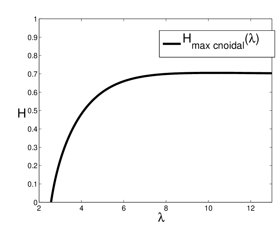
Figure 4 shows a plot of obtained using a finer resolution in than displayed in the table above. It can be seen that the maximum wave height seems to approach zero as approaches zero, which fact is related to a going ’outside’ of the domain of validity of the Boussinesq approximation, where and are assumed to be of the same order of magnitude. It is also worth noting that the limiting values of , and as are:
Applying this to equation (3.4) gives the breaking criterion for the solitary wave, equation (2.5). This is also easy to see if we plot the maximum wave height of the cnoidal wave as a function of wavelength .
4 Numerical study of wave breaking in undular bores

A bore or traveling hydraulic jump is the transition between two uniform flows with different depths. Assuming that one of these flow depths is the undisturbed water level , and the incident water level is given by , we denote by the strength of the bore. With the nondimensionalization explained in the introduction, the undisturbed depth is , and the incident water level is . In this section we aim to find the threshold for which the bore transitions from being purely undular to one which exhibits breaking in the leading wave. This threshold is defined in terms of the ratio , and was found experimentally to be [18].
As already mentioned, if the kinematic breaking criterion is used in connection with phase-resolving numerical models, there is no difficulty in evaluating the local wave and particle velocities. When coupled with the Boussinesq ansatz for the horizontal velocity, the convective criterion allowed for a somewhat accurate description of the breaking of the leading wave behind an undular bore [6]. In this study, numerical integration of a Boussinesq system for undular bores indicated that breaking should occur if the bore strength is greater than . While this result is qualitatively in the right direction, the critical bore strength is overestimated by about . In the following, it will be shown how this result can be improved.
In order to find the critical bore strength in the numerical KdV model, we will therefore use the value of as a starting point, and then proceed with small increments until the breaking criterion is reached, i.e. when the horizontal particle speed of the fluid exceeds the phase speed. The initial position of the bore front will be set to be the origin, and the bore will then travel downstream in the positive -direction. Initial data are given by
| (4.1) |
where is a model parameter denoting the steepness of the initial bore slope. The numerical approach to obtaining approximate solutions of (1.1) with the appropriate boundary conditions is detailed in the appendix.


In order to test the convective breaking criterion (1.6), at each time step the horizontal particle velocity and the phase speed of the bore front have to be calculated numerically. First, given the numerical solution , we approximate the second spatial derivative of the surface, by the second-order central-difference formula
where is the spatial grid size. We then define the approximate horizontal particle velocity at a grid point and time , and evaluated at the free surface as , such that equation (2.2) yields
| (4.2) |
The phase speed of the first wave behind the bore front can be approximated by measuring how the maximum of this wave propagates in time. The left panel of Figure 5 shows the initial profile with and as a dashed curve, and the resulting bore profile at as a solid curve. The figure also shows the horizontal component of the velocity field underneath the first wavecrest, and it is apparent that this bore does not break as the particle velocity remains smaller than the propagation velocity of the leading wave.
After increasing by increments of breaking is obtained for . A computation for (which is already past breaking) is shown in the right panel of figure 5. It can be seen that the horizontal particle velocity is greater than the front velocity after the solution has developed for some time. As expected, the critical bore strength is bigger than the one found experimentally, but is fairly close to the one found in [6].
The maximum waveheight of the solution may be extracted at the particular time step where breaking first occurs. If this waveheight is compared to the critical waveheight of the solitary wave from section 2, it is found that the leading wave behind the bore breaks at a waveheight slightly larger than the solitary wave. However, the values obtained for maximum wave height of the bore seem to approach the maximum height of the solitary wave as the bore strength decreases. Since smaller bore strengths will have larger lead times before the largest wave reaches the point of breaking, in these cases, the leading wave has already separated as an individual solitary wave, and the waveheight at breaking matches closely the value obtained for .
The figure below shows a plot of the calculated values of as a function of time. A curve of the form has also been fitted to the data.


The parameters , and in the fitted curve are given by
and the residual sum of squares is . The curve fits the data fairly well, and it is evident from the form of the equation that it approaches the value for large . This value is very close to the maximum possible height of the solitary wave . We can therefore confirm that the bore eventually disintegrates into several solitary waves, but as the bore strength, , increases, the bore will break before this happens and thus cannot be described in terms of solitary waves. This observation also points to the possibility of obtaining a lower value of the critical bore strength if a similar curve fit is used. To this end, we plot the bore strength as a function of corresponding breaking times. If a curve of the same form as above is used, the parameters , and in the fitted curve are given by
The residual is , and visual inspection of Figure 6 indicates that the fitted curve fits the data rather well also in this case. The numerical value of indicates an asymptotic critical bore strength of for large values of , and this value is somewhat lower than the value of obtained previously.
5 Conclusion
It has been shown that the derivation of the KdV equation as a model for surface water waves admits the definition of a local particle velocity field. The horizontal component of this velocity field may be evaluated near the crest of a wave. For solitary and cnoidal waves, evaluating the local Froude number leads to a convective wave breaking criterion which shows that there is a limiting waveheight beyond which the waves feature incipient wave breaking. Thus even though the solitary wave and the cnoidal waves are solutions of the KdV equation for any waveheight, they do not represent valid approximate surface waves for waveheights beyond the critical waveheight.
The critical waveheight for solitary waves is is quite large, and it is not surprising that these waves do not represent reasonable approximations to real surface waves. For the cnoidal waves, the situation is more complex. For waves near Stokes number , the limiting waveheight according to the convective breaking criterion is in the range to (see Table 1), and these waves are in the range where it is generally thought that solutions of the KdV equation give a faithful approximation of real surface waves. As the elliptic parameter approaches , the critical waveheight of the cnoidal waves approaches . On the other hand, the limit in the case when is the linear case in which solutions have negligible amplitude, and the critical waveheight in this case is indeed .
The convective breaking criterion has also been used to determine the critical bore strength for which an undular bore first exhibits breaking. The result is still somewhat higher than the experimentally determined value , which was obtained using wave tank experiments [18], but lower than the ratio obtained using a similar numerical model in [6]. The discrepancy with the experimental findings could be ascribed to the assumptions made on the physical system, i.e. the absence of transverse motion of the fluid and an irrotational and inviscid flow. While recent studies have highlighted the importance of these effects [13, 29], it is not clear that the inclusion of any of these will improve the quantitative agreement between the current analysis and the experimental findings of [18]. For example frictional damping due to molecular viscosity and boundary effects are more likely to delay the onset of breaking than to facilitate it. It therefore seems likely that the limiting procedure used in obtaining the model equations is responsible for some of the discrepancy, and a possible avenue for improving the quantitative description of wave breaking in an undular bore would be to include some of the higher-order terms which were neglected in the KdV model. Such higher-order models including both nonlinear and dispersive effects are well known (see [20] and the references therein).
Another possible improvement is the relaxation of the breaking criterion
recently advocated in [4, 5].
In these works, several breaking criteria were used
in connection with numerical Boussinesq models,
and with the aim of quantifying the onset of breaking in shoaling waves.
It was found that
the convective criterion (1.6) did not perform as well as other criteria based
on local waveheight [21, 35], and a relaxation constant was introduced in order
to improve the analysis.
However, since this constant has to be determined empirically from a given set of experiments,
we have chosen not to pursue such a development here.
Acknowledgments: This work was supported in part by the Research Council of Norway through grant no. 213474/F20.
Appendix A The numerical scheme for the KdV equation
The numerical approximation of solutions of the equation (1.1) is based on a finite-difference method for the spatial derivatives with appropriate boundary conditions, and a hybrid Adams-Bashforth / Crank-Nicolson time integration scheme. Since the KdV equation is of third order in spatial derivatives, three boundary conditions are needed for the numerical scheme. In the far field downstream of the bore front the surface elevation approaches zero, while in far field upstream it approaches . These far field conditions are chosen to be the boundary conditions which are exact up to machine precision as long as the spatial domain is large enough. Thus care has to be taken to ensure this is the case. For the third boundary condition a homogeneous Neumann condition is chosen on the right. To summarize, the problem to be solved is given by
| (A.1) |
In order to incorporate non-homogeneous boundary conditions, we define the auxiliary function
| (A.2) |
Upon substituting for in (A.1) we have the problem in terms of and which now has homogeneous Dirichlet conditions along with the same homogeneous Neumann condition on the right. The problem (A.1) now reads
where , and homogeneous boundary and initial conditions are imposed.
To approximate the spatial derivatives a finite difference scheme is applied, while to advance in time, an explicit Adams-Bashforth method is used on the nonlinear terms and an implicit Crank-Nicolson method is used on the linear terms. Both methods are of second order, and while this does not automatically yield a second-order scheme for the full equation, numerical experiments in [31] suggest that this is in fact the case.
We continue by discretizing the spatial domain, uniformly using a finite set of points, , where and , and is the distance between two neighboring grid points. The time domain is also discretized uniformly using , where . We define the approximate function value at time and grid point to be . The solutions is then given by (A.2).
The first and third derivatives at a point are approximated as follows using the central difference formulas:
From the Dirichlet conditions we have that and so we need only solve the equation for the grid points . This leaves us with only two points for which the third derivative approximation is not valid. From the Neumann condition we have that , so by writing this as a central difference approximation we get that
This enables us to use the third derivative approximation at grid point as follows
As there is no Neumann condition on the left we use a forward difference formula to approximate the third derivative at grid point :
Defining difference matrices in this way, we may set up the following difference equation:
where and .
By applying the Adams-Bashforth method to the two first terms on the right, and the Crank-Nicolson method to the next two terms we get
At each time step this equation has to be solved for to advance in time. By defining the matrix for convenience, we do this as follows ( denotes the identity matrix):
This method requires function values at two previous time steps to calculate the next one, so at the very first iteration a different approach is needed. One way of fixing the problem is to use a forward Euler method on the nonlinear terms at the first time step. This method has a local truncation error of order two and any instability issues will not be a problem for one single time step. Thus we get the following difference equation for the first time step:
References
- [1] M. Ablowitz and H. Segur, Solitons and the Inverse Scattering Transform, SIAM Studies in Applied Mathematics 4 (SIAM, Philadelphia, 1981).
- [2] A. Ali and H. Kalisch, Mechanical balance laws for Boussinesq models of surface water waves, J. Nonlinear Sci. 22 (2012), 371–398.
- [3] A. Ali and H. Kalisch, On the formulation of mass, momentum and energy conservation in the KdV equation, Acta Appl. Math. 133 (2014), 113–131.
- [4] P. Bacigaluppi, M. Ricchiuto and P. Bonneton, A 1D stabilized finite element model for non-hydrostatic wave breaking and run-up Finite Volumes for Complex Applications VII-Elliptic, Parabolic and Hyperbolic Problems Springer Proceedings in Mathematics & Statistics Vol. 78, 2014, pp 779-790
- [5] P. Bacigaluppi, M. Ricchiuto and P. Bonneton, Upwind stabilized finite element modelling of non-hydrostatic wave breaking and run-up, hal-00990002 (2014).
- [6] M. Bjørkavåg and H. Kalisch, Wave breaking in Boussinesq models for undular bores, Phys. Lett. A 375 (2011), 1570–1578.
- [7] J.L. Bona, M. Chen and J.-C. Saut, Boussinesq equations and other systems for small-amplitude long waves in nonlinear dispersive media. I: Derivation and linear theory, J. Nonlinear Sci. 12 (2002), 283–318.
- [8] J.L. Bona, T. Colin and D. Lannes, Long wave approximations for water waves, Arch. Ration. Mech. Anal. 178 (2005), 373–410.
- [9] J.L. Bona and J.-C. Saut, Dispersive blowup of solutions of generalized Korteweg-de Vries equations, J. Differential Equations 103 (1993), 3–57.
- [10] J.L. Bona, S.M. Sun and B.-Y. Zhang, A nonhomogeneous boundary-value problem for the Korteweg–de Vries equation posed on a finite domain, Comm. Partial Differential Equations 28 (2003), 1391–1436.
- [11] H. Borluk and H. Kalisch, Particle dynamics in the KdV approximation, Wave Motion 49 (2012), 691–709.
- [12] H. Borluk, H. Kalisch and D.P. Nicholls, A numerical study of the Whitham equation as a model for steady surface water waves, J. Comput. Appl. Math. 296 (2016) 293–302.
- [13] H. Chanson, Current knowledge in hydraulic jumps and related phenomena. A survey of experimental results, Europ. J. Mech. B/Fluids 28 (2009), 191–210.
- [14] A. Chawla, H.T. Özkan-Haller and J.T. Kirby, Spectral model for wave transformation and breaking over irregular bathymetry, J. Wtrwy., Port, Coast., and Oc. Engrg 124 (1998), 189-198.
- [15] Y.-Y. Chen, H.-C. Hsu and G.-Y. Chen. Lagrangian experiment and solution for irrotational finite-amplitude progressive gravity waves at uniform depth, Fluid Dynam. Res. 42 045511 (2010) (34pp).
- [16] R.G. Dean and R.A. Dalrymple, Water wave mechanics for engineers and scientists, (World Scientific, Singapore, 1991)
- [17] M.W. Dingemans, Water wave propagation over uneven bottoms: Linear wave propagation. Vol. 13. World Scientific, 1997.
- [18] H. Favre, Ondes de Translation, (Dunod, Paris, 1935).
- [19] D. Henry, Steady periodic flow induced by the Korteweg-de Vries equation, Wave Motion 46, 403–411 (2009).
- [20] A. Karczewska, P. Rozmej and E. Infeld, Energy invariant for shallow-water waves and the Korteweg-de Vries equation: Doubts about the invariance of energy, Phys. Rev. E 92 (2015), 053202.
- [21] M. Kazolea, A. Delis and C. Synolakis, Numerical treatment of wave breaking on unstructured finite volume approximations for extended Boussinesq-type equations, J. Comput. Phys. (2014).
- [22] C. Kharif and E. Pelinovsky, Physical mechanisms of the rogue wave phenomenon, Europ. J. Mech. B/Fluids 22 (2003), 603–634.
- [23] C. Koch and H. Chanson, Unsteady turbulence characteristics in an undular bore, in River Flow 2006, Taylor & Francis Group, London, 2006.
- [24] D.J. Korteweg and G. de Vries, On the change of form of long waves advancing in a rectangular channel and on a new type of long stationary wave, Philos. Mag. 39 (1895), 422–443.
- [25] D. Lannes, The water waves problem (Amer. Math. Soc., Providence, 2013).
- [26] D.F. Lawden. Elliptic functions and applications, (Springer, New York, 1989).
- [27] M.S. Longuet-Higgins, On wave breaking and equilibrium spectrum of wind, Proc. R. Soc. London, Ser. A, 310 (1969), 151–159.
- [28] J. Rauch, Partial Differential Equations, (Springer, New York, 1991).
- [29] G. Richard and S. Gavrilyuk, The classical hydraulic jump in a model of shear shallow-water flows, J. Fluid Mech. 725 (2013), 492–521.
- [30] S. Sato and M.B. Kabiling, A numerical simulation of beach evolution based on a nonlinear dispersive wave-current model, Proceedings of the Twenty-Fourth International Conference held in Kobe, Japan, Coastal Engineering 1994, New York, (1995), 2557-2570.
- [31] J.O. Skogestad and H. Kalisch, A boundary value problem for the KdV equation: Comparison of finite-difference and Chebyshev methods, Math. Comput. Simulation 80 (2009), 151–163.
- [32] P. Stansell and C. MacFarlane, Experimental investigation of wave breaking criteria based on wave phase speeds, J. Phys. Oceanography 32 (2002), 1269–1283.
- [33] Z. Tian, M. Perlin and W. Choi, Evaluation of a deep-water wave breaking criterion, Phys. Fluids 20 (2008), 066604.
- [34] M. Tissier, P. Bonneton, F. Marche, F. Chazel, and D. Lannes, A new approach to handle wave breaking in fully non-linear Boussinesq models, Coast. Engineering 67 (2012), 54–66.
- [35] M. Tonelli and M. Petti, Simulation of wave breaking over complex bathymetries by a Boussinesq model, J. Hydr. Research 49 (2011), 473-486.
- [36] M.P. Tulin and J.J. Li, On the breaking of energetic waves, International J. Offshore Polar Engrng 2 (1992).
- [37] G.B. Whitham, Linear and Nonlinear Waves, Wiley, New York, 1974.
- [38] C.H. Wu and H.M. Nepf, Breaking criteria and energy losses for three‐dimensional wave breaking J. Geophys. Res.: Oceans 107 (2002), C10.
- [39] A. Yao and C.H. Wu, Incipient breaking of unsteady waves on sheared currents, Phys. Fluids 17 (2005), 082104.