跳到论文正文
W Papers独立论文阅读器 arXiv:1603.09071 论文正文 计算阅读时间 · 0%
引用这篇论文根据当前论文元数据生成,正式投稿前建议核对。


License: arXiv.org perpetual non-exclusive license
arXiv:1603.09071v4 [math.ST] 24 Jul 2017

Robust Low-Rank Matrix Estimation

Andreas Elsenerlabel=e1]elsener@stat.math.ethz.ch Email: [    Sara van de Geerlabel=e2]geer@stat.math.ethz.ch Email: [ Affiliation: ETH Zürich Address:  Seminar for Statistics
ETH Zurich
8092 Zurich
Switzerland
Abstract

Many results have been proved for various nuclear norm penalized estimators of the uniform sampling matrix completion problem. However, most of these estimators are not robust: in most of the cases the quadratic loss function and its modifications are used. We consider robust nuclear norm penalized estimators using two well-known robust loss functions: the absolute value loss and the Huber loss. Under several conditions on the sparsity of the problem (i.e. the rank of the parameter matrix) and on the regularity of the risk function sharp and non-sharp oracle inequalities for these estimators are shown to hold with high probability. As a consequence, the asymptotic behavior of the estimators is derived. Similar error bounds are obtained under the assumption of weak sparsity, i.e. the case where the matrix is assumed to be only approximately low-rank. In all our results we consider a high-dimensional setting. In this case, this means that we assume n≤p​qn\leq pq. Finally, various simulations confirm our theoretical results.

Keywords: 
sparsity,
keywords
[class=MSC]
keywords
††email: e1††email: e2

and

1 Introduction

1.1 Background and Motivation

Netflix, Spotify, Apple Music, Amazon and many other on-line services offer an almost infinite amount of songs or films to their users. Clearly, a single person will never be able to watch every film or to listen to every available song. For this reason, an elaborate recommendation system is necessary in order to allow the users to choose content that already match his or her preferences. Many models and estimation methods have been proposed to address this question. Matrices provide an appropriate way of modelling this problem. Imagine that the plethora of films/songs is identified with the rows of a matrix, call it B∗B^{*}, and the users with its columns. One entry of the matrix corresponds to the rating given to film `​`​i​"``i" (row) by user `​`​j​"``j" (column). This matrix will have many missing entries. These entries are bounded and we can expect the rows of B∗B^{*} to be very similar to each other. It is therefore sensible to assume that B∗B^{*} has a low rank. The challenge is now to predict the missing ratings/fill in the empty entries of B∗B^{*}. Define for this purpose the set of observed (possibly noisy) entries

𝒜:={(i,j)∈{1,…,p}×{1,…,q}:the (noisy) entry\displaystyle\mathcal{A}:=\left\{(i,j)\in\left\{1,\dots,p\right\}\times\left\{1,\dots,q\right\}:\mbox{the (noisy) entry}\right. (1.1)
Ai​jofB∗is observed},\displaystyle\left.\ A_{ij}\ \mbox{of}\ B^{*}\ \mbox{is observed}\right\},

where pp is the number of films/songs and qq the number of users. Our estimation problem can therefore be stated in the following way: for B∈ℬ⊂ℝp×qB\in\mathcal{B}\subset\mathbb{R}^{p\times q} we

minimize​Rn​(B),subject to​rank​(B)=s.\mbox{minimize}\ R_{n}(B),\ \mbox{subject to}\ \mbox{rank}(B)=s.

In this special case we have that

ℬ={B∈ℝp×q|‖B‖∞≤η},\mathcal{B}=\left\{B\in\mathbb{R}^{p\times q}|\|B\|_{\infty}\leq\eta\right\}, (1.2)

where η\eta is for instance the mean highest rating, and RnR_{n} is some convex empirical error measure that is defined by the data, e.g.

Rn​(B)=1|𝒜|​∑(i,j)∈𝒜(Ai​j−Bi,j)2.R_{n}(B)=\frac{1}{|\mathcal{A}|}\sum_{(i,j)\in\mathcal{A}}(A_{ij}-B_{i,j})^{2}. (1.3)

Since the rank of a matrix is not convex we use the nuclear norm as its convex surrogate. This leads us to a relaxed convex optimization problem. For B∈ℬB\in\mathcal{B} we

minimize​Rn​(B),subject to​‖B‖nuclear≤τ,\mbox{minimize}\ R_{n}(B),\ \mbox{subject to}\ \|B\|_{\mbox{nuclear}}\leq\tau,

for some τ>0\tau>0. The model described above can be considered as a special case of the trace regression model.

In the trace regression model (see e.g. Rohde and Tsybakov (2011)) one considers the observations (Xi,Yi)(X_{i},Y_{i}) satisfying

Yi=trace(XiB∗)+εi,i=1,…,n,Y_{i}=\trace(X_{i}B^{*})+\varepsilon_{i},\ i=1,\dots,n, (1.4)

where εi\varepsilon_{i} are i.i.d. random errors. The matrices XiX_{i} are so-called masks. They are assumed to lie in

χ={ek(q)el(p)T:1≤k≤q,1≤l≤p},\mathcal{\chi}=\left\{e_{k}(q)e_{l}(p)^{T}:1\leq k\leq q,1\leq l\leq p\right\}, (1.5)

where ek​(q)e_{k}(q) is the qq-dimensional kk-th unit vector and el​(p)e_{l}(p) is the pp-dimensional ll-th unit vector. We will assume that the XiX_{i} are i.i.d. with

ℙ⁡(Xik​j=1)=1−ℙ⁡(Xik​j=0)=1p​q\mathbb{P}\left(X_{i_{kj}}=1\right)=1-\mathbb{P}\left(X_{i_{kj}}=0\right)=\frac{1}{pq}

for all i∈{1,…,n}i\in\left\{1,\dots,n\right\}, k∈{1,…​q}k\in\left\{1,\dots q\right\}, and j∈{1,…,p}j\in\left\{1,\dots,p\right\}. However, we point out that it is not necessary for our estimators to know this distribution. This knowledge will only be used in the proofs of the theoretical results.

The trace regression model together with the space χ\chi and the distribution on χ\chi is equivalent to the matrix completion case. The entries of the vector YY can be identified with the observed entries as those in the matrix AA.

From this, it can be seen that we are in a high-dimensional setting since the number of observations nn must be smaller than or equal to the total number of entries of AA. The setup described above is then called uniform sampling matrix completion. A very similar setup was first considered in Srebro, Rennie and Jaakkola (2005) and Srebro and Shraibman (2005).

As in the standard regression setting, parameter estimation in the trace regression model is also done via empirical risk minimization. Using the Lagrangian form for B∈ℬB\in\mathcal{B} we

minimize​Rn​(B)+λ​‖B‖nuclear,\mbox{minimize}\ R_{n}(B)+\lambda\|B\|_{\mbox{nuclear}},

where Rn(B)=1/n∑i=1nρ(Yi−trace(XiB))R_{n}(B)=1/n\sum_{i=1}^{n}\rho(Y_{i}-\trace(X_{i}B)), ρ\rho is a convex loss function and λ>0\lambda>0 is the tuning parameter. The loss function is often chosen to be the quadratic loss (or one of its modifications) as in Koltchinskii, Lounici and Tsybakov (2011); Negahban and Wainwright (2011); Negahban and Wainwright (2012); Rohde and Tsybakov (2011) and many others. In Lafond (2015) the case of an error distribution belonging to an exponential family is considered. As long as the errors are assumed to be light tailed as it is the case for i.i.d. Gaussian errors the least squares estimator will perform very well. However, the ratings are heavily subject to frauds (e.g. by the producer of a film). It is necessary to take this fact into account also in the estimation procedure. One might also be interested in estimating the median or another quantile of the ratings. For this purpose, M-estimators based on different losses than the quadratic loss are usually chosen.

1.2 Proposed estimators

In this paper, we consider the absolute value loss and the Huber loss. The first robust estimator is then given by

B^:=arg​minB∈ℬ​1n​∑i=1n|Yi−trace⁡(Xi​B)|+λ​‖B‖nuclear.\hat{B}:=\underset{B\in\mathcal{B}}{\argmin}\ \frac{1}{n}\sum_{i=1}^{n}\left|Y_{i}-\trace\left(X_{i}B\right)\right|+\lambda\left\|B\right\|_{\mbox{nuclear}}. (1.6)

Using the Huber loss we can define

B^H:=arg​minB∈ℬ​1n​∑i=1nρH​(Yi−trace⁡(Xi​B))+λ​‖B‖nuclear,\hat{B}_{H}:=\underset{B\in\mathcal{B}}{\argmin}\frac{1}{n}\sum_{i=1}^{n}\rho_{H}\left(Y_{i}-\trace\left(X_{i}B\right)\right)+\lambda\left\|B\right\|_{\mbox{nuclear}}, (1.7)

where the function

ρH​(x):={x2,if​|x|≤κ2​κ​|x|−κ2,if​|x|>κ\rho_{H}(x):=\left\{\begin{array}[]{ll}x^{2},&\mbox{if}\ \left|x\right|\leq\kappa\\ 2\kappa\left|x\right|-\kappa^{2},&\mbox{if}\ \left|x\right|>\kappa\end{array}\right.

defines the Huber loss function. The tuning parameter κ>0\kappa>0 is assumed to be given for our estimation problem. The possible values for the Huber parameter κ\kappa depend on the distribution of the errors as shown in Lemma 2.1. In practice, one usually estimates κ\kappa and λ\lambda with methods such as cross-validation. Notice that it could happen that the estimators defined in Equations 1.6 and 1.7 are not unique since the objective functions are not strictly convex. As will be shown, the rates depend on the Lipschitz constants of the loss functions and on η\eta. Typically, the Lipschitz constants of the absolute value loss as well as of the Huber loss induce smaller constants in the rates compared to the Lipschitz constant of the truncated quadratic loss.

The “target” is defined as

B0:=arg​minB∈ℬ​R​(B),B^{0}:=\underset{B\in\mathcal{B}}{\argmin}\ R(B),

where R⁡(B)=𝔼​Rn​(B)R(B)=\mathbb{E}R_{n}(B) is the theoretical risk. It has to be noticed that the matrix B0B^{0} is not necessarily equal to the matrix B∗B^{*}. Our main interest lies in the theoretical analysis of the above estimators. The estimators should mimic the sparsity behavior of an oracle BB. In the case of the absolute value loss we will prove a non-sharp oracle inequality. Whereas for the Huber loss, thanks to its differentiability, we are able to derive a sharp oracle inequality.

Assuming B=B0B=B^{0} in Corollary 3.1 the upper bound is typically of the form

R⁡(B^H)−R⁡(B0)≲λ2​p​q​s0,R(\hat{B}_{H})-R(B^{0})\lesssim\lambda^{2}pqs_{0}, (1.8)

where ≲\lesssim means that some multiplicative constants (depending on the tuning parameter κ\kappa) are omitted.

The assumptions for this kind of results are mainly based on the regularity of the absolute value and the Huber loss. Moreover, the properties of the nuclear norm, which are very similar to those of the ℓ1\ell_{1}-norm for vectors, will be exploited. In addition, we use the sparsity behavior induced by the nuclear norm to infer the behavior of weakly sparse estimators. This takes into account that a matrix could have few very large singular values and many small, but not exactly zero singular values:

B∈{B′∈ℬ:∑j=1qΛjr≤ρrr,Λ1,…,Λqthe singular values ofB′},\ B\in\left\{B^{\prime}\in\mathcal{B}:\sum_{j=1}^{q}\Lambda_{j}^{r}\leq\rho_{r}^{r},\Lambda_{1},\dots,\Lambda_{q}\ \mbox{the singular values of}\ B^{\prime}\right\},

where 0<r<10<r<1 and ρrr\rho_{r}^{r} is some reasonably small constant.

1.3 Related Literature

A first study with robust matrix estimation was made in Chandrasekaran et al. (2011) in a setting with no missing entries. In order to avoid identifiability issues the authors introduce “incoherence” conditions on the low-rank component. These conditions make sure that the low-rank component itself is not too sparse. The locations of the corruptions are assumed to be fixed. In the context of Principal Component Analysis (PCA) which is a special case of the matrix regression model robustness was investigated in Candès et al. (2011). The authors assume that the matrix to be estimated is decomposed in a low-rank matrix and a sparse matrix. In contrast to Chandrasekaran et al. (2011) the non-zero entries of the sparse matrix are assumed to be drawn randomly following a uniform distribution. Following this line of research Li (2011) apply these conditions to the matrix completion problem with randomly observed entries. In a parallel work Chen et al. (2013) consider the case where the indices of the observed entries may be simultaneously both random and deterministic. In these papers only noiseless robust matrix completion is considered.

Cambier and Absil (2016) study computational aspects of robust matrix completion (in the previously mentioned setting). A method relying on Riemannian optimization is proposed. The authors assume the rank of the matrix to be estimated to be known.

In Foygel et al. (2011) weighted nuclear norm penalized estimators with (possibly nonconvex) Lipschitz continuous loss functions are studied from a learning point of view. The partially observed entries are assumed to follow a possibly non-uniform distribution on the set χ\chi. In contrast, our derivations rely among other properties on the convexity of the risk (i.e. the margin conditions).

Noisy robust matrix completion was first investigated in Klopp, Lounici and Tsybakov (2016). The authors assume that the truth A∗A^{*} is decomposed in a low-rank matrix and a sparse matrix where the low-rank matrix contains the “parameters of interest” and the sparse matrix contains the corruptions. In addition, every observation is corrupted by independent and centered subgaussian noise. The largest entries of both the low-rank and sparse matrices are assumed to be bounded (e.g. by the maximal possible rating). Their model is as follows: (Xi,Y~i),i=1,…​N(X_{i},\tilde{Y}_{i}),i=1,\dots N satisfy

Y~i=trace(XiA∗)+ξi,i=1,…,N,\tilde{Y}_{i}=\trace(X_{i}A^{*})+\xi_{i},i=1,\dots,N, (1.9)

where A∗=L∗+S∗A^{*}=L^{*}+S^{*} with L∗L^{*} a low-rank matrix and S∗S^{*} a matrix with entrywise sparsity. Columnwise sparsity is also considered but in view of a comparison of this and our approach we prefer to restrict to entrywise sparsity. The masks XiX_{i} are assumed to lie in the set χ\chi (1.5) and to be independent of the noise ξi\xi_{i} for all ii. The set of observed indices is assumed to be the union of two disjoint components Ξ\Xi and Ξ~\tilde{\Xi}. The set Ξ\Xi corresponds to the non-corrupted noisy observations (i.e. only entries of L∗L^{*} plus ξi\xi_{i}). The entries corresponding to these observations of S∗S^{*} are zero. The set Ξ~\tilde{\Xi} contains the indices of the observations that are corrupted by a (nonzero) entry of S∗S^{*}. It is not known if an observation comes from Ξ\Xi or Ξ~\tilde{\Xi}. The estimator given in Klopp, Lounici and Tsybakov (2016) is

(L^,S^)∈arg⁡min‖L‖∞≤η‖S‖∞≤η​{1N​∑i=1N(Y~i−trace⁡(Xi​(L+S)))2+λ1​‖L‖nuclear+λ2​‖S‖1}.(\hat{L},\hat{S})\in\underset{\begin{subarray}{c}\|L\|_{\infty}\leq\eta\\ \|S\|_{\infty}\leq\eta\end{subarray}}{\arg\min}\left\{\frac{1}{N}\sum_{i=1}^{N}(\tilde{Y}_{i}-\trace(X_{i}(L+S)))^{2}+\lambda_{1}\|L\|_{\text{nuclear}}+\lambda_{2}\|S\|_{1}\right\}. (1.10)

In contrast to the previously mentioned papers on robust matrix completion, we consider (possibly heavy-tailed) random errors that affect the observations but not the truth.

1.4 Organization of the paper

The paper is organized in the following way. We state the main assumptions that are used throughout the paper in Section 2. Then, the nuclear norm, its properties, and its similarities to the ℓ1\ell_{1}-norm are discussed. To bound the empirical process part resulting from the matrix completion setting we make use of the results in Section B.3 of the Supplementary Material (Appendix B). In Section 3 the main theorems are presented: the (deterministic) sharp and non-sharp oracle inequalities. In Section 3.3 we present the applications of these results to the case of Huber loss and absolute value loss. The asymptotics and the applications to weak sparsity are presented in Section 4. Finally, to verify the theoretical findings, Section 5 presents some simulations. The Student t distribution with three degrees of freedom is considered as an error distribution.

2 Preliminaries

In this section the assumptions on the loss functions, the risk, and the distribution of the errors are presented. In particular, Assumptions 1-3 below are on the curvature of the (theoretical) risk. They are used to derive the deterministic sharp and non-sharp oracle inequalities. It is important to notice that the curvature of the risk mainly depends on the properties of the distribution of the errors. Assumptions 4 and 5 below will be shown to be sufficient for Assumptions 2 and 3 to hold, respectively.

Furthermore, we also discuss the properties of the nuclear norm. Thanks to the penalization term in the objective functions the optimization problems become computationally tractable. We also highlight the commonalities of the vector ℓ1\ell_{1}-norm and the nuclear norm for matrices.

2.1 Assumptions on the risk and the distribution of the errors

The first assumption is about the loss function.

Assumption 1.

Let ρ\rho be the loss function. We assume that it is Lipschitz continuous with constant LL, i.e. that for all x,y∈ℝx,y\in\mathbb{R}

|ρ⁡(x)−ρ⁡(y)|≤L​|x−y|.|\rho(x)-\rho(y)|\leq L|x-y|. (2.1)

The next two assumptions ensure the identifiability of the parameters by requiring a sufficient convexity of the risk around the target.

Assumption 2.

One-point-margin condition. There is an increasing strictly convex function GG with G⁡(0)=0G(0)=0 such that for all B∈ℬB\in\mathcal{B}

R⁡(B)−R⁡(B0)≥G⁡(‖B−B0‖F),R\left(B\right)-R\left(B^{0}\right)\geq G\left(\|B-B^{0}\|_{F}\right),

where RR is the theoretical risk function.

Assumption 3.

Two-point-margin condition. There is an increasing strictly convex function GG with G⁡(0)=0G(0)=0 such that for all B,B′∈ℬB,B^{\prime}\in\mathcal{B} we have

R⁡(B)−R⁡(B′)≥trace⁡(R˙​(B′)T​(B−B′))+G⁡(‖B−B′‖F),R\left(B\right)-R\left(B^{\prime}\right)\geq\trace\left(\dot{R}\left(B^{\prime}\right)^{T}\left(B-B^{\prime}\right)\right)+G\left(\|B-B^{\prime}\|_{F}\right),

where RR is the theoretical risk function and [R˙​(B′)]k​l=∂∂Bk​l​R​(B)|B=B′[\dot{R}(B^{\prime})]_{kl}=\frac{\partial}{\partial B_{kl}}R(B)|_{B=B^{\prime}}.

Assumption 1 is crucial when it comes to the application of the Contraction Theorem which in turn allows us to apply the dual norm inequality to find a bound for the random part of the oracle bounds. Assumptions 2 and 3 are essential in the proofs of the (deterministic) results. In particular, in addition to the differentiability of the empirical risk RnR_{n}, Assumption 3 is responsible for the sharpness of the first oracle bound that will be proved. The margin conditions are strongly related to the shape of the distribution function and the corresponding density of the errors.

For the specific application to the Huber loss and absolute value loss estimators we show that mild conditions on the distribution of the errors ensure a sufficient curvature of the risk for both loss functions under study.

Assumption 3 holds under a weak condition on the distribution function of the errors:

Assumption 4.

Assume that there exists a constant C1>0C_{1}>0 such that the distribution function FF with density with respect to Lebesgue measure ff of the errors fulfills

F⁡(u+κ)−F⁡(u−κ)≥1/C12,for all​|u|≤2​η​and​κ≤2​η.F(u+\kappa)-F(u-\kappa)\geq 1/C_{1}^{2},\ \mbox{for all}\ |u|\leq 2\eta\ \mbox{and}\ \kappa\leq 2\eta. (2.2)
Lemma 2.1.

Assumption 4 implies Assumption 3 with G⁡(u)=u2/(2​C12​p​q)G(u)=u^{2}/(2C_{1}^{2}pq).

The following assumption guarantees that Assumption 2 holds.

Assumption 5.

Suppose ε1,…,εn\varepsilon_{1},\dots,\varepsilon_{n} are i.i.d. with median zero and density ff with respect to Lebesgue measure. Assume that for C2>0C_{2}>0

f⁡(u)≥1C22,for all​|u|≤2​η.f\left(u\right)\geq\frac{1}{C_{2}^{2}},\ \mbox{for all}\ \left|u\right|\leq 2\eta. (2.3)
Lemma 2.2.

Assumption 5 implies Assumption 2 with G⁡(u)=u2/(2​C22​p​q)G(u)=u^{2}/(2C_{2}^{2}pq).

Another important fact is that when the distribution of the errors is assumed to be symmetric around zero B∗=B0B^{*}=B^{0}. This phenomenon is discussed in Section 4 of the Supplement.

2.2 Properties of the nuclear norm

The regularization by the nuclear norm plays a similar role as the ℓ1\ell_{1}-norm in the Lasso (Tibshirani, 1996). We illustrate the similarities and differences of these types of regularizations. In view of the oracle inequalities and in order to keep the notation as simple as possible we discuss the properties of the nuclear norm of the oracle. The oracle is typically a value BB that takes an up-to-constants optimal trade-off between approximation error and estimation error. In what follows, BB is called “the oracle” although its choice is flexible.

Consider the singular value decomposition of the oracle BB with rank s⋆s^{\star} given by

B=P​Λ​QT,B=P\Lambda Q^{T}, (2.4)

where PP is a p×qp\times q matrix, QQ a q×pq\times p matrix and Λ\Lambda a q×qq\times q diagonal matrix containing the ordered singular values Λ1≥⋯≥Λq\Lambda_{1}\geq\dots\geq\Lambda_{q}. Then the nuclear norm is given by

‖B‖nuclear=∑i=1qΛi​(B)=‖Λ⁡(B)‖1,\left\|B\right\|_{\mbox{nuclear}}=\sum_{i=1}^{q}\Lambda_{i}(B)=\left\|\Lambda(B)\right\|_{1}, (2.5)

by interpreting Λ⁡(B)∈ℝq\Lambda(B)\in\mathbb{R}^{q} as the vector of singular values. The penalization with the nuclear norm induces sparsity in the singular values, whereas the penalization with the vector ℓ1\ell_{1}-norm of the parameters in linear regression induces sparsity directly in the parameters. On the other hand, the rank plays the role of the number of non-zero coefficients in the Lasso setting, namely

s⋆=‖Λ⁡(B)‖0.s^{\star}=\left\|\Lambda(B)\right\|_{0}. (2.6)

One main ingredient of the proofs of the oracle inequalities is the so-called triangle property as introduced in van de Geer (2001). This property was used in e.g. Bühlmann and van de Geer (2011) to prove non-sharp oracle inequalities. For the ℓ1\ell_{1}-norm the triangle property follows from its decomposability. For the nuclear norm the triangle property as it is used in this work depends on the features of the oracle BB. For this reason we notice that for any positive integer s≤qs\leq q the oracle can be decomposed in

B=B++B−,B+=∑k=1sΛk​Pk​QkT,B−=∑k=s+1qΛk​Pk​QkT.B=B^{+}+B^{-},\quad B^{+}=\sum_{k=1}^{s}\Lambda_{k}P_{k}Q_{k}^{T},\quad B^{-}=\sum_{k=s+1}^{q}\Lambda_{k}P_{k}Q_{k}^{T}.

The matrix B+B^{+} is called “active” part of the oracle BB, whereas the matrix B−B^{-} is called the “non-active” part. The singular value decomposition of B+B^{+} is given by

B+=P+ΛQ+T.B^{+}=P^{+}\Lambda Q^{+^{T}}.

We observe that the integer ss is not necessarily the rank of the oracle BB. The choice of ss is free. One may choose a value that trades off the roles of the “active” part B+B^{+} and “non-active” part B−B^{-}, see Lemma 4.1. The following lemma is adapted from Lemma 7.2 and Lemma 12.5 in van de Geer (2016).

Lemma 2.3.

Let B+∈ℝp×qB^{+}\in\mathbb{R}^{p\times q} be the active part of the oracle BB. Then we have for all B′∈ℝp×qB^{\prime}\in\mathbb{R}^{p\times q} with

ΩB++​(B′)\displaystyle\Omega^{+}_{B^{+}}\left(B^{\prime}\right) :=s(‖P+P+TB′‖F+‖B′Q+Q+T‖F+‖P+P+TB′Q+Q+T‖F)\displaystyle:=\sqrt{s}\left(\left\|P^{+}P^{+^{T}}B^{\prime}\right\|_{F}+\left\|B^{\prime}Q^{+}Q^{+^{T}}\right\|_{F}+\left\|P^{+}P^{+^{T}}B^{\prime}Q^{+}Q^{+^{T}}\right\|_{F}\right)
and
ΩB+−​(B′)\displaystyle\Omega_{B^{+}}^{-}\left(B^{\prime}\right) :=‖(I−P+P+T)B′(I−Q+Q+T)‖nuclear\displaystyle:=\left\|\left(I-P^{+}P^{+^{T}}\right)B^{\prime}\left(I-Q^{+}Q^{+^{T}}\right)\right\|_{\mbox{\emph{nuclear}}}

that

‖B+‖ nuclear−‖B′‖nuclear≤ΩB++​(B′−B+)−ΩB+−​(B′).\left\|B^{+}\right\|_{\mbox{ \emph{nuclear}}}-\left\|B^{\prime}\right\|_{\mbox{\emph{nuclear}}}\leq\Omega_{B^{+}}^{+}\left(B^{\prime}-B^{+}\right)-\Omega_{B^{+}}^{-}\left(B^{\prime}\right). (2.7)

We then say that the triangle property holds at B+B^{+}.

In particular, since ΩB++​(B−)=0\Omega_{B^{+}}^{+}(B^{-})=0, we have for any B′∈ℝp×qB^{\prime}\in\mathbb{R}^{p\times q}

‖B‖nuclear−‖B′‖nuclear≤ΩB++​(B′−B)−ΩB+−​(B′−B)+2​‖B−‖nuclear.\left\|B\right\|_{\mbox{\emph{nuclear}}}-\left\|B^{\prime}\right\|_{\mbox{\emph{nuclear}}}\leq\Omega^{+}_{B^{+}}(B^{\prime}-B)-\Omega^{-}_{B^{+}}(B^{\prime}-B)+2\left\|B^{-}\right\|_{\mbox{\emph{nuclear}}}. (2.8)

Moreover, we have

‖⋅‖nuclear≤ΩB+++ΩB+−.\left\|\cdot\right\|_{\mbox{\emph{nuclear}}}\leq\Omega_{B^{+}}^{+}+\Omega_{B^{+}}^{-}. (2.9)

From now on, we write Ω+=ΩB++\Omega^{+}=\Omega_{B^{+}}^{+} and Ω−=ΩB+−\Omega^{-}=\Omega_{B^{+}}^{-}. Equation 2.8 is proved in Appendix A.

Hence, the property that our estimators should mimic is not the rank of the oracle but rather the fact that the “non-active” part is zero under the semi-norm induced by the active part.

Moreover, we define the norm Ω¯\underline{\Omega} as

Ω¯:=Ω++Ω−.\underline{\Omega}:=\Omega^{+}+\Omega^{-}.
Remark 1.

Notice that the semi-norms Ω+\Omega^{+} and Ω−\Omega^{-} form a complete pair, meaning that Ω¯:=Ω++Ω−\underline{\Omega}:=\Omega^{+}+\Omega^{-} is a norm.

The estimation error in several different norms can thus be “computed” in general (semi-)norms.

A tail bound for the maximal singular value of a finite sum of matrices lying in the set χ\chi defined in Equation (1.5) is given in the following theorem. For this purpose, we first need to define the Orlicz norm of a random variable. Let Z∈ℝZ\in\mathbb{R} be a random variable and α≥1\alpha\geq 1 a constant. Then the Ψα−\Psi_{\alpha}-Orlicz norm is defined as

‖Z‖Ψα:=inf{c>0:𝔼​exp⁡[|Z|α/cα]≤2}\left\|Z\right\|_{\Psi_{\alpha}}:=\inf\left\{c>0:\mathbb{E}\exp\left[\left|Z\right|^{\alpha}/c^{\alpha}\right]\leq 2\right\} (2.10)
Theorem 2.1 ( Proposition 2 in Koltchinskii, Lounici and Tsybakov (2011) ).

Let X1,…,XnX_{1},\dots,X_{n} be i.i.d. q×pq\times p matrices that satisfy for some α≥1\alpha\geq 1 (and all ii)

𝔼​Xi=0,‖Λmax​(Xi)‖Ψα=:K<∞.\mathbb{E}X_{i}=0,\left\|\Lambda_{\max}(X_{i})\right\|_{\Psi_{\alpha}}=:K<\infty.

Define

S2:=max⁡{Λmax​(∑i=1n𝔼​Xi​XiT)/n,Λmax​(∑i=1n𝔼​XiT​Xi)/n}.S^{2}:=\max\left\{\Lambda_{\max}\left(\sum_{i=1}^{n}\mathbb{E}X_{i}X_{i}^{T}\right)/n,\Lambda_{\max}\left(\sum_{i=1}^{n}\mathbb{E}X_{i}^{T}X_{i}\right)/n\right\}.

Then for a constant CC and for all t>0t>0

ℙ⁡(Λmax​(∑i=1nXi)/n≥C​S​t+log⁡(p+q)nCLOSE\displaystyle\mathbb{P}\left(\Lambda_{\max}\left(\sum_{i=1}^{n}X_{i}\right)/n\geq CS\sqrt{\frac{t+\log(p+q)}{n}}\right.
OPEN+C​log1/α⁡(KS)​(t+log⁡(p+q)n))≤exp⁡(−t).\displaystyle\left.+C\log^{1/\alpha}\left(\frac{K}{S}\right)\left(\frac{t+\log(p+q)}{n}\right)\right)\leq\exp(-t).

This theorem is used with the tail summation property of the expectation in the derivations of the tail bounds in Section 3 of the Supplementary Material.

3 Oracle inequalities

We first give two deterministic sharp and non-sharp oracle inequalities. The connection to the empirical process parts and to the specific loss functions follows in Subsection 3.3. Let B0=arg​minB′∈ℬ​R​(B′)B^{0}=\underset{B^{\prime}\in\mathcal{B}}{\argmin}\ R(B^{\prime}) be the target. It is assumed that q≤pq\leq p.

3.1 Sharp oracle inequality

Here, we assume that the loss function is differentiable and Lipschitz continuous. The next lemma gives a connection between the empirical risk and the penalization term.

Lemma 3.1 (adapted from Lemma 7.1 in van de Geer (2016)).

Suppose that RnR_{n} is differentiable. Then for all B∈ℬB\in\mathcal{B}

−trace⁡(R˙n​(B^)T​(B−B^))≤λ​‖B‖nuclear−λ​‖B^‖nuclear.-\trace\left(\dot{R}_{n}(\hat{B})^{T}(B-\hat{B})\right)\leq\lambda\|B\|_{\mbox{\emph{nuclear}}}-\lambda\|\hat{B}\|_{\mbox{\emph{nuclear}}}.

The following theorem is inspired by Theorem 7.1 in van de Geer (2016). In contrast to this theorem, we need to bound the empirical process part differently. In view of the application to the matrix completion problem, we assume a specific bound on the empirical process.

Theorem 3.1.

Suppose that Assumptions 1 and 3 hold, that the loss function is differentiable, and let HH be the convex conjugate of GG. Assume further for all B′∈ℬB^{\prime}\in\mathcal{B} that for λε>0\lambda_{\varepsilon}>0 and λ∗>0\lambda_{*}>0

|trace⁡((R˙n​(B′)−R˙​(B′))T​(B−B′))|≤λε​Ω¯​(B′−B)+λ∗.\left|\trace\left(\left(\dot{R}_{n}\left(B^{\prime}\right)-\dot{R}\left(B^{\prime}\right)\right)^{T}\left(B-B^{\prime}\right)\right)\right|\leq\lambda_{\varepsilon}\underline{\Omega}(B^{\prime}-B)+\lambda_{*}.

Take λ>λε\lambda>\lambda_{\varepsilon}. Let 0≤δ<10\leq\delta<1 be arbitrary, and define

λ¯:=λ−λε,λ¯:=λε+λ+δ​λ¯\underline{\lambda}:=\lambda-\lambda_{\varepsilon},\quad\overline{\lambda}:=\lambda_{\varepsilon}+\lambda+\delta\underline{\lambda}

Then

δ​λ¯​Ω+​(B^−B)+δ​λ¯​Ω−​(B^−B)+R⁡(B^)−R⁡(B)\displaystyle\delta\underline{\lambda}\Omega^{+}(\hat{B}-B)+\delta\underline{\lambda}\Omega^{-}(\hat{B}-B)+R(\hat{B})-R(B)
≤H⁡(λ¯​3​s)+2​λ​‖B−‖nuclear+λ∗.\displaystyle\leq H(\overline{\lambda}3\sqrt{s})+2\lambda\left\|B^{-}\right\|_{\mbox{\emph{nuclear}}}+\lambda_{*}.

In the proof of this theorem the differentiability of the loss function and Assumption 3 are crucial. Without this property an additional term arising from the one-point-margin condition would appear in the upper bound. This term would then lead to a non-sharp bound.

3.2 Non-sharp oracle inequality

Instead of bounding an empirical process term depending on the derivative of the empirical and theoretical risks we need to consider differences of these functions.

Theorem 3.2.

Suppose that Assumptions 1 and 2 hold. Let HH be the convex conjugate of GG. Suppose further that for λε>0\lambda_{\varepsilon}>0, λ∗>0\lambda_{*}>0, and all B′∈ℬB^{\prime}\in\mathcal{B}

|[Rn​(B′)−R⁡(B′)]−[Rn​(B)−R⁡(B)]|≤λε​Ω¯​(B′−B)+λ∗.\left|\left[R_{n}(B^{\prime})-R(B^{\prime})\right]-\left[R_{n}(B)-R(B)\right]\right|\leq\lambda_{\varepsilon}\underline{\Omega}(B^{\prime}-B)+\lambda_{*}. (3.1)

Let 0<δ<10<\delta<1, take λ>λε\lambda>\lambda_{\varepsilon} and define

λ¯=λ+λε,λ¯=λ−λε.\overline{\lambda}=\lambda+\lambda_{\varepsilon},\quad\underline{\lambda}=\lambda-\lambda_{\varepsilon}. (3.2)

Then,

δ​λ¯​Ω¯​(B^−B)\displaystyle\delta\underline{\lambda}\underline{\Omega}(\hat{B}-B) ≤2​H​(λ¯​(1+δ)​3​s)\displaystyle\leq 2H(\overline{\lambda}(1+\delta)3\sqrt{s})
+2​(λ∗+(R⁡(B)−R⁡(B0)))+4​λ​‖B−‖nuclear\displaystyle\phantom{\dots}+2\left(\lambda_{*}+(R(B)-R(B^{0}))\right)+4\lambda\|B^{-}\|_{\mbox{\emph{nuclear}}}

and

R⁡(B^)−R⁡(B)\displaystyle R(\hat{B})-R(B) ≤1δ[2H(λ¯(1+δ)3s)+λ∗+2(R(B)−R(B0))\displaystyle\leq\frac{1}{\delta}\left[2H(\overline{\lambda}(1+\delta)3\sqrt{s})+\lambda_{*}+2(R(B)-R(B^{0}))\right.
+2λ∥B−∥nuclear]+λ∗+2λ∥B−∥nuclear.\displaystyle\phantom{\leq}\left.+2\lambda\|B^{-}\|_{\mbox{\emph{nuclear}}}\right]+\lambda_{*}+2\lambda\|B^{-}\|_{\mbox{\emph{nuclear}}}.

It has to be noticed that the above bound is “good” only if R⁡(B)−R⁡(B0)R(B)-R(B^{0}) is already small. The main cause for the non-sharpness is Assumption 2 that leads to an additional term in the upper bound of the inequality.

3.3 Applications to specific loss functions

We now apply the deterministic sharp and non-sharp oracle inequalities to the case of the Huber loss and absolute value loss, respectively. We assume in both cases that the distribution of the errors is symmetric around 00 so that B0=B∗B^{0}=B^{*}. This is discussed in detail in Section B.4.

Huber Loss-sharp oracle inequality

We first consider the case that arises by choosing the Huber loss. Theorem 3.1 together with Lemma 2.1 and the first claim of Lemma 3.2 in the Supplement imply the following corollary. It is useful to notice that the Lipschitz constant of the Huber loss is 2​κ2\kappa.

Corollary 3.1.

Let B=B++B−B=B^{+}+B^{-} where B+B^{+} and B−B^{-} are defined in Equation 2.4. Let Assumption 4 be satisfied.

For a constant C0>0C_{0}>0 let

λε=2​(4​η+2​κ)​((8​C0+2)​log⁡(p+q)n​q+8​C0​log⁡(1+q)​log⁡(p+q)n)\displaystyle\lambda_{\varepsilon}=2(4\eta+2\kappa)\left((8C_{0}+\sqrt{2})\sqrt{\frac{\log(p+q)}{nq}}+8C_{0}\sqrt{\log(1+q)}\frac{\log(p+q)}{n}\right)

and λ∗=8​η​(4​η+2​κ)​p​log⁡(p+q)/(3​n)+λε\lambda_{*}=8\eta(4\eta+2\kappa)p\log(p+q)/(3n)+\lambda_{\varepsilon}.

Assume that λ>λε\lambda>\lambda_{\varepsilon}. Take 0≤δ<10\leq\delta<1,

λ¯:=λ−λε​and​λ¯:=λε+λ+δ​λ¯\underline{\lambda}:=\lambda-\lambda_{\varepsilon}\ \mbox{and}\ \overline{\lambda}:=\lambda_{\varepsilon}+\lambda+\delta\underline{\lambda} (3.3)

Choose j0:=⌈log2⁡(7​q​p​q​η)⌉j_{0}:=\lceil\log_{2}(7q\sqrt{pq}\eta)\rceil and define

α=(j0+2)​exp⁡(−p​log⁡(p+q)).\alpha=(j_{0}+2)\exp(-p\log(p+q)).

Then we have with probability at least 1−α1-\alpha that

δ​λ¯​Ω+​(B^H−B)+δ​λ¯​Ω−​(B^H−B)+R⁡(B^H)−R⁡(B)\displaystyle\delta\underline{\lambda}\Omega^{+}(\hat{B}_{H}-B)+\delta\underline{\lambda}\Omega^{-}(\hat{B}_{H}-B)+R(\hat{B}_{H})-R(B)
≤p​q​C12​λ¯2​9​s2+2​λ​‖B−‖nuclear+λ∗.\displaystyle\leq\frac{pqC_{1}^{2}\bar{\lambda}^{2}9s}{2}+2\lambda\left\|B^{-}\right\|_{\mbox{\emph{nuclear}}}+\lambda_{*}.

Assumption 4 guarantees that the risk function is sufficiently convex. From this assumption we also obtain a bound for the possible values of the tuning parameter κ\kappa. We can also see that the results hold for errors with a heavier tail than the Gaussian. The choice of the noise level λε\lambda_{\varepsilon} and consequently of the tuning parameter λ\lambda results from the the probability inequalities for the empirical process in Section B.3. The quantity λ∗\lambda_{*} is also a consequence of the bound on the empirical process part. However, it does not affect the asymptotic rates.

Absolute value loss - non-sharp oracle inequality

The next corollary is an application to the case of the absolute value loss. Theorem 3.2 combined with Lemma 2.2 and the second claim of Lemma 3.2 in the Supplement lead to the following corollary. The Lipschitz constant in this case is 11.

Corollary 3.2.

Let the oracle BB be as in 2.4. Suppose that Assumption 5 is satisfied. For a constant C0>0C_{0}>0 let

λε=2​((8​C0+2)​log⁡(p+q)n​q+8​C0​log⁡(1+q)​log⁡(p+q)n)\displaystyle\lambda_{\varepsilon}=2\left((8C_{0}+\sqrt{2})\sqrt{\frac{\log(p+q)}{nq}}+8C_{0}\sqrt{\log(1+q)}\frac{\log(p+q)}{n}\right)

and λ∗=8​η​p​log⁡(p+q)/(3​n)+λε\lambda_{*}=8\eta p\log(p+q)/(3n)+\lambda_{\varepsilon}. Take 0<δ<10<\delta<1 and λ>λε\lambda>\lambda_{\varepsilon}. Choose j0:=⌈log2⁡(7​q​p​q​η)⌉j_{0}:=\lceil\log_{2}(7q\sqrt{pq}\eta)\rceil and define

α=(j0+2)​exp⁡(−p​log⁡(p+q)).\alpha=(j_{0}+2)\exp(-p\log(p+q)).

Then we have with probability at least 1−α1-\alpha that

δ​λ¯​Ω¯​(B^−B)\displaystyle\delta\underline{\lambda}\underline{\Omega}(\hat{B}-B)
≤6​C2​λ¯2​(1+δ)2​p​q​s+2​λ∗+2​(R⁡(B)−R⁡(B0))+4​λ​‖B−‖nuclear\displaystyle\leq 6C^{2}\overline{\lambda}^{2}\left(1+\delta\right)^{2}pqs+2\lambda_{*}+2(R(B)-R(B^{0}))+4\lambda\|B^{-}\|_{\mbox{\emph{nuclear}}}

and

R⁡(B^)−R⁡(B)\displaystyle R(\hat{B})-R(B) ≤1δ[6C22λ¯2(1+δ)2pqs+λ∗+2(R(B)−R(B0))\displaystyle\leq\frac{1}{\delta}\Big[6C_{2}^{2}\overline{\lambda}^{2}\left(1+\delta\right)^{2}pqs+\lambda_{*}+2(R(B)-R(B^{0}))
+2λ∥B−∥nuclear]+λ∗+2λ∥B−∥nuclear.\displaystyle\phantom{\leq\frac{1}{\delta}}+2\lambda\|B^{-}\|_{\mbox{\emph{nuclear}}}\Big]+\lambda_{*}+2\lambda\|B^{-}\|_{\mbox{\emph{nuclear}}}.

Also in this case, the choices of λε\lambda_{\varepsilon} and λ∗\lambda_{*} are a consequence of the probability bounds.

4 Asymptotics and Weak sparsity

The results in Section 3 are valid for finite values of the dimension of the matrix p,qp,q, the rank, and the number of observed entries nn. A question that is answered in this section is how the estimation errors of the proposed estimators behave when n,p,n,p, and qq are allowed to grow.

As mentioned in Negahban and Wainwright (2012), practical reasons motivate the assumption that the matrix B0B^{0} is not exactly low-rank but only approximately. In relation to the matrix completion problem one observes that the ratings given by the users are unlikely to be exactly equal but rather very similar. This translates to a matrix that is not low-rank. However, it is sensible to assume that the matrix is almost low-rank. The notion of weak sparsity quantifies this assumption by assuming that for some 0<r<10<r<1 and ρ>0\rho>0

∑k=1q(Λk0)r=:ρrr,\sum_{k=1}^{q}\left(\Lambda_{k}^{0}\right)^{r}=:\rho_{r}^{r}, (4.1)

where Λ10,…,Λq0\Lambda_{1}^{0},\dots,\Lambda_{q}^{0} are the singular values of B0B^{0}. For r=0r=0 we have under the convention that 00=00^{0}=0 that

∑k=1q(Λk0)0=∑k=1q𝟙{Λk0>0}=s0,\sum_{k=1}^{q}\left(\Lambda_{k}^{0}\right)^{0}=\sum_{k=1}^{q}\mathbbm{1}_{\left\{\Lambda_{k}^{0}>0\right\}}=s_{0},

where s0s_{0} is the rank of B0B^{0}. The following lemma gives a bound of the non-active part of the matrix BB that appears in the oracle bounds.

Lemma 4.1.

For σ>0\sigma>0 we may take

‖B−‖nuclear≤σ1−r​ρrr,\left\|B^{-}\right\|_{\mbox{\emph{nuclear}}}\leq\sigma^{1-r}\rho_{r}^{r}, (4.2)

and

s≤σ−r​ρrr.s\leq\sigma^{-r}\rho_{r}^{r}.

We first consider the asymptotic behavior of our estimators in the case of an exactly low-rank matrix and deduce from this the asymptotics for the case of an approximately low-rank matrix.

4.1 Asymptotics

4.1.1 sharp

By Corollary 3.1, assuming that q​log⁡(1+q)=o⁡(nlog⁡(p+q))q\log(1+q)=o\left(\frac{n}{\log(p+q)}\right), and therefore using the choice for the noise level

λε≍log⁡(p+q)n​q\lambda_{\varepsilon}\asymp\sqrt{\frac{\log(p+q)}{nq}}

we obtain

R⁡(B^H)−R⁡(B0)\displaystyle R(\hat{B}_{H})-R(B^{0}) ≤R⁡(B)−R⁡(B0)\displaystyle\leq R(B)-R(B^{0})
+𝒪ℙ​(p​s​log⁡(p+q)n+log⁡(p+q)n​q​(1+‖B−‖nuclear)).\displaystyle\phantom{\dots}+\mathcal{O}_{\mathbb{P}}\left(\frac{ps\log(p+q)}{n}+\sqrt{\frac{\log(p+q)}{nq}}\left(1+\left\|B^{-}\right\|_{\mbox{nuclear}}\right)\right). (4.3)

We choose for simplicity the oracle to be the matrix B0B^{0} itself with s0=rank​(B0)s_{0}=\mbox{rank}(B^{0}). Then, we make use of the two point margin condition that is shown to hold in Lemma 2.1.The resulting rate is then given by

‖B^H−B0‖F2=𝒪ℙ​((4​η+2​κ)2​C14​p2​q​s0​log⁡(p+q)n),\|\hat{B}_{H}-B^{0}\|_{F}^{2}=\mathcal{O}_{\mathbb{P}}\left((4\eta+2\kappa)^{2}C_{1}^{4}\frac{p^{2}qs_{0}\log(p+q)}{n}\right), (4.4)

where κ\kappa is the Huber parameter and C1C_{1} is the constant from Lemma 2.1.

Remark 2.

The rate (4.4) depends on η\eta as in Koltchinskii, Lounici and Tsybakov (2011) and on the Lipschitz constant of the loss function which is typically smaller than η\eta. If C12=O⁡(η)C_{1}^{2}=O(\eta), the constant in front of the rate is of order O⁡(η4)O(\eta^{4}). This is a “worst-case” scenario that shows the cost that is paid when allowing for very general error distributions as in our case. We emphasize that in this case the distribution of the errors is not required to have a density.

In addition to the rate obtained for the Frobenius norm, we are also able to derive rates for the estimation error measured in nuclear norm. From Corollary 3.1 and Equation 2.9 under the previous conditions it follows that

‖B^H−B0‖nuclear=𝒪ℙ​(C12​p​q​s0​log⁡(p+q)n​q).\|\hat{B}_{H}-B^{0}\|_{\text{nuclear}}=\mathcal{O}_{\mathbb{P}}\left(C_{1}^{2}pqs_{0}\sqrt{\frac{\log(p+q)}{nq}}\right). (4.5)

4.1.2 non-sharp

By Corollary 3.2 it is known that the assumption q​log⁡(1+q)=o⁡(nlog⁡(p+q))q\log(1+q)=o\left(\frac{n}{\log(p+q)}\right) leads to the choice λε≍log⁡(p+q)/n​q\lambda_{\varepsilon}\asymp\sqrt{\log(p+q)/nq}. Therefore, we have

R⁡(B^)−R⁡(B0)\displaystyle R(\hat{B})-R(B^{0})
=𝒪ℙ​(p​s​log⁡(p+q)n+R⁡(B)−R⁡(B0)+log⁡(p+q)n​q​(1+‖B−‖nuclear)).\displaystyle=\mathcal{O}_{\mathbb{P}}\left(\frac{ps\log(p+q)}{n}+R\left(B\right)-R\left(B^{0}\right)+\sqrt{\frac{\log(p+q)}{nq}}(1+\left\|B^{-}\right\|_{\mbox{nuclear}})\right). (4.6)

What can be observed comparing the rates in Equations (4.3) and (4.6) is the presence of the additional term R⁡(B)−R⁡(B0)R(B)-R(B^{0}) in the non-sharp case in contrast to the sharp case. We choose again the oracle to be the matrix B0B^{0} itself. By the one point margin condition derived in Lemma 2.2 we see that the rate of convergence in this case is given by

‖B^−B0‖F2=𝒪ℙ​(C24​p2​q​s0​log⁡(p+q)n),\|\hat{B}-B^{0}\|_{F}^{2}=\mathcal{O}_{\mathbb{P}}\left(C_{2}^{4}\frac{p^{2}qs_{0}\log(p+q)}{n}\right), (4.7)

where the constant C2C_{2} comes from Lemma 2.2.

Remark 3.

If C22=O⁡(η)C_{2}^{2}=O(\eta) a comparison with the rates obtained in Koltchinskii, Lounici and Tsybakov (2011) shows that the rates agree. In contrast to the rate obatined for the Huber loss (Equation 4.4), the distribution of the errors is assumed to have a density. This leads to a constant of order O⁡(η2)O(\eta^{2}) in a “worst-case” scenario. It is a natural consequence of the stronger assumption on the distribution of the errors. This is comparable to the constant obtained in Koltchinskii, Lounici and Tsybakov (2011).

In analogy to the previous case, we are able to derive a rate for the estimation error measured in nuclear norm:

‖B^−B0‖nuclear=𝒪ℙ​(C22​p​q​s0​log⁡(p+q)n​q).\|\hat{B}-B^{0}\|_{\text{nuclear}}=\mathcal{O}_{\mathbb{P}}\left(C_{2}^{2}pqs_{0}\sqrt{\frac{\log(p+q)}{nq}}\right). (4.8)

The rates are indeed very slow but this is not surprising given that per entry the number of observations is about n/(p​q)n/(pq). The price to pay for the estimation of the reduced number of parameters p​s0ps_{0} is given by the term log⁡(p+q)\log(p+q).

4.2 Weak sparsity

In what follows, the asymptotic behavior of the proposed estimators is discussed when applied to an estimation problem where one aims at estimating a matrix that is not exactly low-rank. With Lemma 4.1 and the rates given in the previous section we are able to derive an explicit rate also for the approximatley low-rank case. For this purpose, we assume that Equation 4.1 holds.

4.2.1 Huber estimator

The following corollary gives rates for the estimation error of the Huber estimator when used for estimation of a not exactly low-rank matrix.

Corollary 4.1.

With q​log⁡(1+q)=o⁡(nlog⁡(p+q))q\log(1+q)=o\left(\frac{n}{\log(p+q)}\right) we choose

λε≍log⁡(p+q)n​q.\lambda_{\varepsilon}\asymp\sqrt{\frac{\log(p+q)}{nq}}.

We then have

‖B^H−B0‖F2=𝒪ℙ​((η+κ)2​C14​p2​q​log⁡(p+q)n)1−r​ρrr.\left\|\hat{B}_{H}-B^{0}\right\|_{F}^{2}=\mathcal{O}_{\mathbb{P}}\left((\eta+\kappa)^{2}C_{1}^{4}\frac{p^{2}q\log(p+q)}{n}\right)^{1-r}\rho_{r}^{r}.

4.2.2 Absolute value estimator

Using the oracle inequality under the weak sparsity assumption we obtain the following result.

Corollary 4.2.

With q​log⁡(1+q)=o⁡(nlog⁡(p+q))q\log(1+q)=o\left(\frac{n}{\log(p+q)}\right) we choose

λε\displaystyle\lambda_{\varepsilon} ≍log⁡(p+q)n​q.\displaystyle\asymp\sqrt{\frac{\log(p+q)}{nq}}.

Then we have for the Frobenius norm of the estimation error

‖B^−B0‖F2=𝒪ℙ​(p2​q​log⁡(p+q)n)1−r​ρrr.\left\|\hat{B}-B^{0}\right\|_{F}^{2}=\mathcal{O}_{\mathbb{P}}\left(\frac{p^{2}q\log(p+q)}{n}\right)^{1-r}\rho_{r}^{r}. (4.9)

5 Simulations

In this section, the robustness of the Huber estimator 1.7 is empirically demonstrated. In Subsection 5.3, the Huber estimator is compared with the estimator proposed in Klopp, Lounici and Tsybakov (2016) under model 1.4 and 1.9 with each Student t and standard Gaussian noise. The sample size ranges in all simulations for all dimensions considered here from 3​p​log⁡(p)​s03p\log(p)s_{0} to p​qpq. Between minimal and maximal sample size there are in each case 1010 points. To illustrate the rate derived in Section 4 we compute the error ‖B^H−B0‖F2\|\hat{B}_{H}-B^{0}\|_{F}^{2} for different dimensions of the problem under increasing number of observations.

To compute the solution of the optimization problem 1.7 functions from the Matlab library cvx (CVX Research, 2012) were used.

Throughout this section the error is assumed to have the following shape

Error=1p​q​‖B^H−B0‖F2=1p​q​∑i=1p∑j=1q(B^Hi​j−Bi​j0)2.\mbox{Error}=\frac{1}{pq}\left\|\hat{B}_{H}-B^{0}\right\|_{F}^{2}=\frac{1}{pq}\sum_{i=1}^{p}\sum_{j=1}^{q}\left(\hat{B}_{H_{ij}}-B_{ij}^{0}\right)^{2}. (5.1)

To verify the robustness of the estimator 1.7 and the rate of convergence that was derived in Section 4 we use the Student t distribution with 33 degrees of freedom. Every point in the plots corresponds to an average of 2525 simulations. The value of the tuning parameter is set to

λ=2​log⁡(p+q)n​q.\lambda=2\sqrt{\frac{\log(p+q)}{nq}}.

A comparison with λε\lambda_{\varepsilon} from Corollary 3.1 indicates that λ\lambda is rather small. For the settings we consider in this section we found that this value for λ\lambda is more appropriate. As done in Candès and Plan (2010), for a better comparison between the error curves of our estimator and the oracle rate in Equation (4.4) this rate was multiplied with 1.681.68 in the case of Student t distributed errors and with 1.11.1 in the case of Gaussian errors.

5.1 t-distributed and gaussian errors

The variance of the Student t distribution with ν>2\nu>2 degrees of freedom is given by

Var⁡(εi)=νν−2,for​εi∼tν.\Var\left(\varepsilon_{i}\right)=\frac{\nu}{\nu-2},\ \mbox{for}\ \varepsilon_{i}\sim t_{\nu}. (5.2)

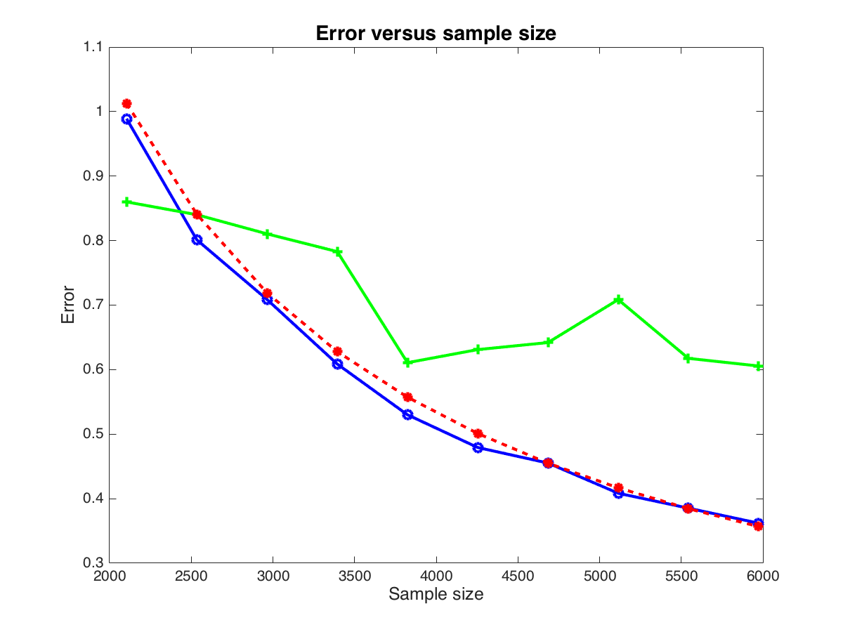
Figure 1(a) shows a comparison between the Huber estimator 1.7 with the estimator that uses the quadratic loss in the case of Student t with 33 degrees of freedom distributed errors. As expected, the estimator that uses the quadratic loss is not robust against the corrupted entries. On the other hand, we can see in Figure 1(b) that the Huber estimator performs almost as well as the quadratic loss estimator in the case of Gaussian errors with variance 11. In agreement with the theory, the rate of the estimator is very close to the oracle rate for sufficiently large sample sizes. The value of κ\kappa that we used in the simulations is 1.3451.345. The maximal rating η\eta is chosen to be η=10\eta=10.

Refer to caption
(a)
Refer to caption
(b)
Figure 1: Comparison of the Huber and quadratic loss in the case of Student t distributed (left figure) and Gaussian errors (right figure). We choose p=q=80p=q=80 and s0=2s_{0}=2. The dot-dashed red line corresponds to 1.681.68 multiplied with the oracle bound derived in Equation 4.4 for the exact low-rank case.

5.2 Changing the problem size

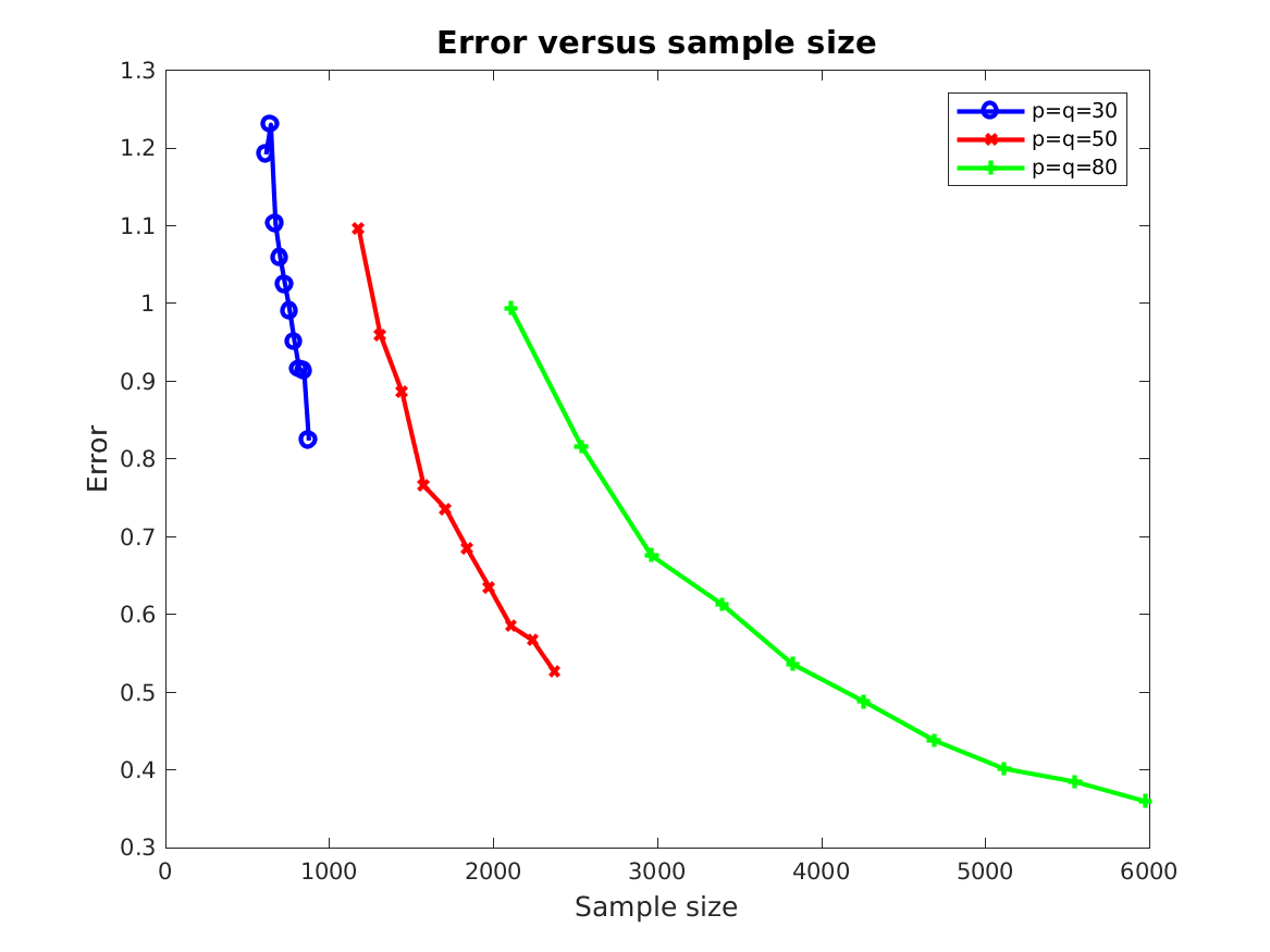
In order to confirm/verify the theoretical results, we proceed similarly to what was done in Negahban and Wainwright (2011) and Negahban and Wainwright (2012) in the corresponding cases. Here, we consider three different problem sizes: p,q∈{30,50,80}p,q\in\left\{30,50,80\right\}. In Figure 2(a) we observe that as the problem gets harder, i.e. as the dimension of the matrix increases, also the sample size needs to be larger. Figure 2(b) shows that by rescaling the sample size by n/(3​p​s0​log⁡(p))n/(3ps_{0}\log(p)) the rate of convergence agrees very well with the theoretical one. It is assumed that the rank of the matrices is s0=2s_{0}=2 for all cases. Every point corresponds to an average of 2525 simulations. The maximal rating η\eta and the tuning parameter κ\kappa are chosen as before.

Refer to caption
(a)
Refer to caption
(b)
Figure 2: Three different problem sizes are considered: p=q∈{30,50,80}p=q\in\left\{30,50,80\right\}. The rank is fixed to s0=2s_{0}=2 in both cases. In Panel (b) it can be seen that the rate of convergence corresponds approximately to the theoretical one derived in Equation 4.4. The dot-dashed line is the oracle. It was multiplied by 1.681.68 in order to fit our curves.

5.3 Comparison with a low-rank + sparse estimator

In this subsection, we compare the performance of the Huber estimator 1.7 with the performance of the low-rank matrix estimator proposed by Klopp, Lounici and Tsybakov (2016) 1.10. We first compare the estimators B^H\hat{B}_{H} and L^\hat{L} with the observations YiY_{i} generated according to the model 1.4 with standard Gaussian and Student t with 33 degrees of freedom distributed errors. Equation (21) in Klopp, Lounici and Tsybakov (2016) suggests that the tuning parameters are chosen as follows:

λ1=2​log⁡(p+q)n​q,λ2=2​log⁡(p+q)n,\lambda_{1}=2\sqrt{\frac{\log(p+q)}{nq}},\quad\lambda_{2}=2\frac{\log(p+q)}{n},

where λ1\lambda_{1} and λ2\lambda_{2} are the tuning parameters of the estimator 1.10. Also in this case it has to be noticed that the tuning parameters are smaller than the theoretical values given in their paper.

Refer to caption
(a)
Refer to caption
(b)
Figure 3: The left panel shows the Huber estimator 1.7 and the low-rank plus sparse estimator 1.10 under the model 1.4 with Student t noise with 33 degrees of freedom. The right panel shows the same estimators under the same model with standard Gaussian noise.

In Figure 3(a) the Huber estimator 1.7 is compared with the low-rank plus sparse estimator 1.10 under the model 1.4 with i.i.d. Student t noise with 33 degrees of freedom. As expected, these estimators perform comparably well under the trace regression model 1.4. In Figure 3(b) the same estimators are compared under the model 1.4 with i.i.d. standard Gaussian noise. Also in this case, we see that both estimators achieve approximately the same error. These observations are not surprising since the theoretical analysis of Section 3 could be carried over by adapting the (semi-)norms to the different penalization.

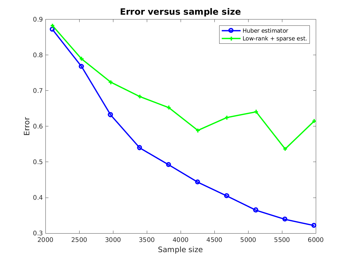
We now consider the model proposed in Klopp, Lounici and Tsybakov (2016) where around 5%5\% of the observed entries are taken to be only one rating. This is the case of malicious users who systematically rate only one particular movie with the same rating. We refer to Section 2.3 of Klopp, Lounici and Tsybakov (2016) for more details on this setting. In Figure 4(a) we see that the Huber estimator outperforms the low-rank plus sparse estimator with Student t noise with 33 degrees of freedom. This might be due to the quadratic loss function and to the choice of the tuning parameters. In Figure 4(b) where Gaussian noise is considered we observe that both estimators perform almost equally well.
Refer to caption
(a)
Refer to caption
(b)
Figure 4: The left panel shows the Huber estimator 1.7 and the low-rank plus sparse estimator 1.10 under the model 1.9 with Student t noise with 33 degrees of freedom. The right panel shows the same estimators under the same model as on the left panel but with standard Gaussian noise.

6 Discussion

In this paper, we have derived sharp and non-sharp oracle inequalities for two robust nuclear norm penalized estimators of the noisy matrix completion problem. The robust estimators were defined using the well-known Huber loss for which the sharp oracle inequality has been derived and the absolute value loss for which we have shown a non-sharp oracle inequality. For both types of oracle inequalities we proved a general deterministic result first and added then the part arising from the empirical process. We have also shown how to apply the oracle inequalities to the case where we only assume weak sparsity, i.e. approximately low-rank matrices. It is worth pointing out that our estimators do not require the distribution on the set of matrices (1.5) to be known in contrast to e.g. Koltchinskii, Lounici and Tsybakov (2011). In our case, the distribution on the set of matrices (1.5) is only needed in the theoretical analysis. The proofs of the oracle inequalities rely on the properties of the nuclear norm, and for the empirical process part on the Concentration, Symmetrization, and Contraction Theorems. A main tool in this context was also the bound on the largest singular value of a matrix with finite Orlicz norm. Our simulations, in the case of the Huber loss, showed a very good agreement with the convergence rates obtained by our theoretical analysis. We saw that the oracle rate is attained up to constants in presence of non-Gaussian noise and that the robust estimation procedure outperforms the quadratic loss function.

It is left to future research to establish a sharp oracle inequality also for the case of a non-differentiable robust loss function. The Contraction inequality used in this paper for the Huber loss requires that also the derivative of the loss is Lipschitz continuous. This is not the case for the absolute value loss. Thanks to the convexity of the loss function it might be possible to derive a sharp result also for this case.

Appendix A Proofs of main results

Proof of Inequality 2.8.

Using the triangle property at B+B^{+} with B′=B+B^{\prime}=B^{+} we obtain

0=‖B+‖nuclear−‖B+‖nuclear≤Ω+​(B+−B+)⏟=0−Ω−​(B+)\displaystyle 0=\|B^{+}\|_{\mbox{nuclear}}-\|B^{+}\|_{\mbox{nuclear}}\leq\underbrace{\Omega^{+}(B^{+}-B^{+})}_{=0}-\Omega^{-}(B^{+})
⇒Ω−​(B+)=0.\displaystyle\Rightarrow\Omega^{-}(B^{+})=0.

By the triangle property at B+B^{+} with B′=B=B++B−B^{\prime}=B=B^{+}+B^{-} we have that

‖B+‖nuclear−‖B‖nuclear\displaystyle\|B^{+}\|_{\mbox{nuclear}}-\|B\|_{\mbox{nuclear}}
=‖B+‖nuclear−‖B++B−‖nuclear\displaystyle=\|B^{+}\|_{\mbox{nuclear}}-\|B^{+}+B^{-}\|_{\mbox{nuclear}}
≤Ω+​(B−)−Ω−​(B++B−)\displaystyle\leq\Omega^{+}(B^{-})-\Omega^{-}(B^{+}+B^{-})
=−Ω−​(B++B−).\displaystyle=-\Omega^{-}(B^{+}+B^{-}).

By the triangle inequality it follows using Ω−​(B+)=0\Omega^{-}(B^{+})=0 that

Ω−​(B++B−)≥Ω−​(B−)−Ω−​(B+)=Ω−​(B−).\Omega^{-}(B^{+}+B^{-})\geq\Omega^{-}(B^{-})-\Omega^{-}(B^{+})=\Omega^{-}(B^{-}).

Therefore, we have

‖B+‖nuclear−‖B++B−‖nuclear≤−Ω−​(B−),\|B^{+}\|_{\mbox{nuclear}}-\|B^{+}+B^{-}\|_{\mbox{nuclear}}\leq-\Omega^{-}(B^{-}),

and by the triangle inequality

‖B+‖nuclear−‖B++B−‖nuclear≥−‖B−‖nuclear,\|B^{+}\|_{\mbox{nuclear}}-\|B^{+}+B^{-}\|_{\mbox{nuclear}}\geq-\|B^{-}\|_{\mbox{nuclear}},

which gives

Ω−​(B−)≤‖B−‖nuclear.\Omega^{-}(B^{-})\leq\|B^{-}\|_{\mbox{nuclear}}.

For an arbitrary BB we have again by the triangle inequality

‖B‖nuclear−‖B′‖nuclear≤‖B+‖nuclear+‖B−‖nuclear−‖B′‖nuclear.\|B\|_{\mbox{nuclear}}-\|B^{\prime}\|_{\mbox{nuclear}}\leq\|B^{+}\|_{\mbox{nuclear}}+\|B^{-}\|_{\mbox{nuclear}}-\|B^{\prime}\|_{\mbox{nuclear}}.

Applying the triangle property at B+B^{+} we find that

‖B‖nuclear−‖B′‖nuclear≤Ω+​(B+−B′)−Ω−​(B′)+‖B−‖nuclear.\|B\|_{\mbox{nuclear}}-\|B^{\prime}\|_{\mbox{nuclear}}\leq\Omega^{+}(B^{+}-B^{\prime})-\Omega^{-}(B^{\prime})+\|B^{-}\|_{\mbox{nuclear}}.

Apply now twice the triangle inequality (first inequality) to find that

‖B‖nuclear−‖B′‖nuclear\displaystyle\|B\|_{\mbox{nuclear}}-\|B^{\prime}\|_{\mbox{nuclear}} ≤Ω+​(B−B′)+Ω+​(B−)−Ω−​(B−B′)\displaystyle\leq\Omega^{+}(B-B^{\prime})+\Omega^{+}(B^{-})-\Omega^{-}(B-B^{\prime})
+Ω−​(B)+‖B−‖nuclear\displaystyle\phantom{\leq}+\Omega^{-}(B)+\|B^{-}\|_{\mbox{nuclear}}
≤Ω+​(B−B′)−Ω−​(B−B′)\displaystyle\leq\Omega^{+}(B-B^{\prime})-\Omega^{-}(B-B^{\prime})
+2​‖B−‖nuclear,\displaystyle\phantom{\leq}+2\|B^{-}\|_{\mbox{nuclear}},

where it was used that Ω⁡(B−)=0\Omega(B^{-})=0 and that Ω−​(B)≤Ω−​(B−)≤‖B−‖nuclear\Omega^{-}(B)\leq\Omega^{-}(B^{-})\leq\|B^{-}\|_{\mbox{nuclear}}. ∎

Proof of Lemma 3.1.

Let B∈ℬB\in\mathcal{B}. Define for 0<t<10<t<1

B~t:=(1−t)​B^+t​B.\tilde{B}_{t}:=(1-t)\hat{B}+tB.

Since ℬ\mathcal{B} is convex we have that B~t∈ℬ\tilde{B}_{t}\in\mathcal{B} for all 0<t<10<t<1. Since B^\hat{B} is the minimizer of the objective function and by the convexity of the objective function we have

Rn​(B^)+λ​‖B^‖nuclear\displaystyle R_{n}(\hat{B})+\lambda\|\hat{B}\|_{\mbox{nuclear}} ≤Rn​(B~t)+λ​‖B~t‖nuclear\displaystyle\leq R_{n}(\tilde{B}_{t})+\lambda\|\tilde{B}_{t}\|_{\mbox{nuclear}}
≤Rn​(B~t)+(1−t)​λ​‖B^‖nuclear+t​λ​‖B‖nuclear.\displaystyle\leq R_{n}(\tilde{B}_{t})+(1-t)\lambda\|\hat{B}\|_{\mbox{nuclear}}+t\lambda\|B\|_{\mbox{nuclear}}.

Finally, we can conclude that

Rn​(B^)−Rn​(B~t)t≤λ​‖B‖nuclear−λ​‖B^‖nuclear.\frac{R_{n}(\hat{B})-R_{n}(\tilde{B}_{t})}{t}\leq\lambda\|B\|_{\mbox{nuclear}}-\lambda\|\hat{B}\|_{\mbox{nuclear}}.

Letting t→0t\rightarrow 0 the claim follows. ∎

Proof of Theorem 3.1.

The first order Taylor expansion of RR at B^\hat{B} is given by

R⁡(B)=R⁡(B^)+trace⁡(R˙​(B^)T​(B−B^))+R​e​m​(B^,B).R(B)=R(\hat{B})+\trace\left(\dot{R}(\hat{B})^{T}(B-\hat{B})\right)+Rem(\hat{B},B). (A.1)

Then it follows that

R⁡(B^)−R⁡(B)+R​e​m​(B^,B)=−trace⁡(R˙​(B^)T​(B−B^)).R(\hat{B})-R(B)+Rem(\hat{B},B)=-\trace\left(\dot{R}(\hat{B})^{T}(B-\hat{B})\right). (A.2)

Case 1

If

trace⁡(R˙​(B^)T​(B−B^))\displaystyle\trace\left(\dot{R}(\hat{B})^{T}(B-\hat{B})\right)
≥δ​λ¯​Ω+​(B^−B)+δ​λ¯​Ω−​(B^−B)−2​λ​‖B−‖nuclear−λ∗,\displaystyle\geq\delta\underline{\lambda}\Omega^{+}(\hat{B}-B)+\delta\underline{\lambda}\Omega^{-}(\hat{B}-B)-2\lambda\|B^{-}\|_{\mbox{nuclear}}-\lambda_{*}, (A.3)

then by the two-point-margin condition 3 we find that

R⁡(B)−R⁡(B^)≥trace⁡(R˙​(B^)T​(B−B^))+G⁡(‖B−B^‖F).R(B)-R(\hat{B})\geq\trace\left(\dot{R}(\hat{B})^{T}(B-\hat{B})\right)+G(\|B-\hat{B}\|_{F}). (A.4)

Which implies that

R⁡(B)−R⁡(B^)\displaystyle R(B)-R(\hat{B}) ≥δ​λ¯​Ω+​(B^−B)+δ​λ¯​Ω−​(B^−B)−2​λ​‖B−‖nuclear\displaystyle\geq\delta\underline{\lambda}\Omega^{+}(\hat{B}-B)+\delta\underline{\lambda}\Omega^{-}(\hat{B}-B)-2\lambda\|B^{-}\|_{\mbox{nuclear}}
−λ∗+G⁡(‖B−B^‖F)⏟≥0\displaystyle\phantom{\geq}-\lambda_{*}+\underbrace{G(\|B-\hat{B}\|_{F})}_{\geq 0}
≥δ​λ¯​Ω+​(B^−B)+δ​λ¯​Ω−​(B^−B)−2​λ​‖B−‖nuclear−λ∗.\displaystyle\geq\delta\underline{\lambda}\Omega^{+}(\hat{B}-B)+\delta\underline{\lambda}\Omega^{-}(\hat{B}-B)-2\lambda\|B^{-}\|_{\mbox{nuclear}}-\lambda_{*}.

Case 2

Assume in the following that

trace⁡(R˙​(B^)T​(B−B^))\displaystyle\trace\left(\dot{R}(\hat{B})^{T}(B-\hat{B})\right)
≤δ​λ¯​Ω+​(B^−B)+δ​λ¯​Ω−​(B^−B)−2​λ​‖B−‖nuclear−λ∗,\displaystyle\leq\delta\underline{\lambda}\Omega^{+}(\hat{B}-B)+\delta\underline{\lambda}\Omega^{-}(\hat{B}-B)-2\lambda\|B^{-}\|_{\mbox{nuclear}}-\lambda_{*}, (A.5)

By the two-point inequality (Lemma 3.1) we have that

−trace⁡(R˙n​(B^)T​(B−B^))≤λ​‖B‖nuclear−λ​‖B^‖nuclear,-\trace\left(\dot{R}_{n}(\hat{B})^{T}(B-\hat{B})\right)\leq\lambda\|B\|_{\mbox{nuclear}}-\lambda\|\hat{B}\|_{\mbox{nuclear}}, (A.6)

which implies that

0≤trace⁡(R˙n​(B^)T​(B−B^))+λ​‖B‖nuclear−λ​‖B^‖nuclear.0\leq\trace\left(\dot{R}_{n}(\hat{B})^{T}(B-\hat{B})\right)+\lambda\|B\|_{\mbox{nuclear}}-\lambda\|\hat{B}\|_{\mbox{nuclear}}. (A.7)

Hence,

−trace⁡(R˙​(B^)T​(B−B^))+δ​λ¯​Ω+​(B^−B)+δ​λ¯​Ω−​(B^−B)\displaystyle-\trace\left(\dot{R}(\hat{B})^{T}(B-\hat{B})\right)+\delta\underline{\lambda}\Omega^{+}(\hat{B}-B)+\delta\underline{\lambda}\Omega^{-}(\hat{B}-B)
≤trace⁡((R˙n​(B^)−R˙​(B^))T​(B−B^))+δ​λ¯​Ω+​(B^−B)+δ​λ¯​Ω−​(B^−B)\displaystyle\leq\trace\left((\dot{R}_{n}(\hat{B})-\dot{R}(\hat{B}))^{T}(B-\hat{B})\right)+\delta\underline{\lambda}\Omega^{+}(\hat{B}-B)+\delta\underline{\lambda}\Omega^{-}(\hat{B}-B)
+λ​‖B‖nuclear−λ​‖B^‖nuclear\displaystyle\phantom{\leq}+\lambda\|B\|_{\mbox{nuclear}}-\lambda\|\hat{B}\|_{\mbox{nuclear}}
≤λε​Ω¯​(B^−B)+λ∗+δ​λ¯​Ω+​(B^−B)+δ​λ¯​Ω−​(B^−B)\displaystyle\leq\lambda_{\varepsilon}\underline{\Omega}(\hat{B}-B)+\lambda_{*}+\delta\underline{\lambda}\Omega^{+}(\hat{B}-B)+\delta\underline{\lambda}\Omega^{-}(\hat{B}-B)
+λ​‖B‖nuclear−λ​‖B^‖nuclear\displaystyle\phantom{\leq}+\lambda\|B\|_{\mbox{nuclear}}-\lambda\|\hat{B}\|_{\mbox{nuclear}}
≤λε​Ω+​(B^−B)+λε​Ω−​(B^−B)+λ∗+δ​λ¯​Ω+​(B^−B)\displaystyle\leq\lambda_{\varepsilon}\Omega^{+}(\hat{B}-B)+\lambda_{\varepsilon}\Omega^{-}(\hat{B}-B)+\lambda_{*}+\delta\underline{\lambda}\Omega^{+}(\hat{B}-B)
+δ​λ¯​Ω−​(B^−B)+λ​Ω+​(B^−B)−λ​Ω−​(B^−B)+2​λ​‖B−‖nuclear\displaystyle\phantom{\leq}+\delta\underline{\lambda}\Omega^{-}(\hat{B}-B)+\lambda\Omega^{+}(\hat{B}-B)-\lambda\Omega^{-}(\hat{B}-B)+2\lambda\|B^{-}\|_{\mbox{nuclear}}
=λ¯​Ω+​(B^−B)−(1−δ)​λ¯​Ω−​(B^−B)+2​λ​‖B−‖nuclear+λ∗.\displaystyle=\overline{\lambda}\Omega^{+}(\hat{B}-B)-(1-\delta)\underline{\lambda}\Omega^{-}(\hat{B}-B)+2\lambda\|B^{-}\|_{\mbox{nuclear}}+\lambda_{*}.

Therefore, by Equation A.5

Ω−​(B^−B)≤λ¯(1−δ)​λ¯​Ω+​(B^−B).\Omega^{-}(\hat{B}-B)\leq\frac{\overline{\lambda}}{(1-\delta)\underline{\lambda}}\Omega^{+}(\hat{B}-B).

We then have by the convex conjugate inequality

Ω+​(B^−B)\displaystyle\Omega^{+}(\hat{B}-B) ≤‖B^−B‖F​3​s\displaystyle\leq\|\hat{B}-B\|_{F}3\sqrt{s}
≤H⁡(3​s)+G⁡(‖B^−B‖F).\displaystyle\leq H\left(3\sqrt{s}\right)+G(\|\hat{B}-B\|_{F}).

Which implies that

−trace⁡(R˙​(B^)T​(B−B^))+λ¯​Ω−​(B^−B)+δ​λ¯​Ω+​(B^−B)\displaystyle-\trace\left(\dot{R}(\hat{B})^{T}(B-\hat{B})\right)+\underline{\lambda}\Omega^{-}(\hat{B}-B)+\delta\underline{\lambda}\Omega^{+}(\hat{B}-B)
=R⁡(B^)−R⁡(B)+R​e​m​(B^,B)+λ¯​Ω−​(B^−B)+δ​λ¯​Ω+​(B^−B)\displaystyle=R(\hat{B})-R(B)+Rem(\hat{B},B)+\underline{\lambda}\Omega^{-}(\hat{B}-B)+\delta\underline{\lambda}\Omega^{+}(\hat{B}-B)
≤H⁡(λ¯​3​s)+G⁡(‖B^−B‖F)+2​λ​‖B−‖nuclear+λ∗\displaystyle\leq H\left(\overline{\lambda}3\sqrt{s}\right)+G(\|\hat{B}-B\|_{F})+2\lambda\|B^{-}\|_{\mbox{nuclear}}+\lambda_{*}
≤H⁡(λ¯​3​s)+R​e​m​(B^,B)+2​λ​‖B−‖nuclear+λ∗.\displaystyle\leq H\left(\overline{\lambda}3\sqrt{s}\right)+Rem(\hat{B},B)+2\lambda\|B^{-}\|_{\mbox{nuclear}}+\lambda_{*}.

∎

Proof of Theorem 3.2.

We start the proof with the following inequality using the fact that B^\hat{B} is the minimizer of the objective function.

Rn​(B^)+λ​‖B^‖nuclear≤Rn​(B)+λ​‖B‖nuclearR_{n}(\hat{B})+\lambda\|\hat{B}\|_{\mbox{nuclear}}\leq R_{n}(B)+\lambda\left\|B\right\|_{\mbox{nuclear}} (A.8)

Then, by adding and subtracting R⁡(B^)R(\hat{B}) on the left hand side and R⁡(B)R(B) on the right hand side we obtain

R⁡(B^)−R⁡(B)\displaystyle R(\hat{B})-R(B) ≤−[(Rn(B^)−R(B^)−(Rn(B)−R(B))]\displaystyle\leq-\left[(R_{n}(\hat{B})-R(\hat{B})-(R_{n}(B)-R(B))\right]
+λ​‖B‖nuclear−λ​‖B^‖nuclear.\displaystyle\phantom{\leq}+\lambda\|B\|_{\mbox{nuclear}}-\lambda\|\hat{B}\|_{\mbox{nuclear}}.

Applying Assumption 3.1, the definition of Ω¯\underline{\Omega}, and Lemma 2.8 we obtain

R⁡(B^)−R⁡(B)≤λε​Ω¯​(B^−B)+λ∗+λ​‖B‖nuclear−λ​‖B^‖nuclear\displaystyle R(\hat{B})-R(B)\leq\lambda_{\varepsilon}\underline{\Omega}(\hat{B}-B)+\lambda_{*}+\lambda\|B\|_{\mbox{nuclear}}-\lambda\|\hat{B}\|_{\mbox{nuclear}}
≤λε​Ω+​(B^−B)+λε​Ω−​(B^−B)+λ∗\displaystyle\leq\lambda_{\varepsilon}\Omega^{+}(\hat{B}-B)+\lambda_{\varepsilon}\Omega^{-}(\hat{B}-B)+\lambda_{*}
+λ​Ω+​(B^−B)−λ​Ω−​(B^−B)+2​λ​‖B−‖nuclear\displaystyle\phantom{\leq}+\lambda\Omega^{+}(\hat{B}-B)-\lambda\Omega^{-}(\hat{B}-B)+2\lambda\|B^{-}\|_{\mbox{nuclear}}
=(λε+λ)​Ω+​(B^−B)−(λ−λε)​Ω−​(B^−B)+λ∗+2​λ​‖B−‖nuclear.\displaystyle=(\lambda_{\varepsilon}+\lambda)\Omega^{+}(\hat{B}-B)-(\lambda-\lambda_{\varepsilon})\Omega^{-}(\hat{B}-B)+\lambda_{*}+2\lambda\|B^{-}\|_{\mbox{nuclear}}.

Since later on we apply Assumption 2 we subtract on both sides of the above inequality R⁡(B0)R(B^{0}).

R⁡(B^)−R⁡(B0)+λ¯​Ω−​(B^−B)\displaystyle R(\hat{B})-R(B^{0})+\underline{\lambda}\Omega^{-}(\hat{B}-B)
≤R⁡(B)−R⁡(B0)+λ¯​Ω+​(B^−B)+λ∗+2​λ​‖B−‖nuclear.\displaystyle\leq R(B)-R(B^{0})+\overline{\lambda}\Omega^{+}(\hat{B}-B)+\lambda_{*}+2\lambda\|B^{-}\|_{\mbox{nuclear}}. (A.9)

It is then useful to make the following case distinction that allows us to obtain an upper bound for the estimation error.
Case 1
If λ¯​Ω+​(B^−B)≤(1−δ)δ​(λ∗+R⁡(B)−R⁡(B0)+2​λ​‖B−‖nuclear)\overline{\lambda}\Omega^{+}(\hat{B}-B)\leq\frac{(1-\delta)}{\delta}\left(\lambda_{*}+R(B)-R(B^{0})+2\lambda\|B^{-}\|_{\mbox{nuclear}}\right), then

δ​λ¯​Ω+​(B^−B)\displaystyle\delta\overline{\lambda}\Omega^{+}(\hat{B}-B) ≤(1−δ)​(λ∗+R⁡(B)−R⁡(B0)+2​λ​‖B−‖nuclear)\displaystyle\leq(1-\delta)\left(\lambda_{*}+R(B)-R(B^{0})+2\lambda\|B^{-}\|_{\mbox{nuclear}}\right)
≤λ∗+R⁡(B)−R⁡(B0)+2​λ​‖B−‖nuclear.\displaystyle\leq\lambda_{*}+R(B)-R(B^{0})+2\lambda\|B^{-}\|_{\mbox{nuclear}}.

By multiplying Equaiton A.9 on both sides with δ\delta we arrive at

δ​λ¯​Ω−​(B^−B)≤λ∗+R⁡(B)−R⁡(B0)+2​λ​‖B−‖nuclear.\displaystyle\delta\underline{\lambda}\Omega^{-}(\hat{B}-B)\leq\lambda_{*}+R(B)-R(B^{0})+2\lambda\|B^{-}\|_{\mbox{nuclear}}.

Therefore,

δ⁡(λ¯​Ω+​(B^−B)+λ¯​Ω−​(B^−B))\displaystyle\delta(\overline{\lambda}\Omega^{+}(\hat{B}-B)+\underline{\lambda}\Omega^{-}(\hat{B}-B))
≤2​λ∗+2​(R⁡(B)−R⁡(B0))+4​λ​‖B−‖nuclear.\displaystyle\leq 2\lambda_{*}+2(R(B)-R(B^{0}))+4\lambda\|B^{-}\|_{\mbox{nuclear}}. (A.10)

And since

λ¯<λ¯,\underline{\lambda}<\overline{\lambda},

we conclude that

δ​λ¯​(Ω++Ω−)​(B^−B)≤2​λ∗+2​(R⁡(B)−R⁡(B0))+4​λ​‖B−‖nuclear.\delta\underline{\lambda}(\Omega^{+}+\Omega^{-})(\hat{B}-B)\leq 2\lambda_{*}+2(R(B)-R(B^{0}))+4\lambda\|B^{-}\|_{\mbox{nuclear}}.

Case 2
If λ¯​Ω+​(B^−B)≥(1−δ)δ​(λ∗+R⁡(B)−R⁡(B0)+2​λ​‖B−‖nuclear)\overline{\lambda}\Omega^{+}(\hat{B}-B)\geq\frac{(1-\delta)}{\delta}\left(\lambda_{*}+R(B)-R(B^{0})+2\lambda\|B^{-}\|_{\mbox{nuclear}}\right), then

R⁡(B^)−R⁡(B0)+λ¯​Ω−​(B^−B)\displaystyle R(\hat{B})-R(B^{0})+\underline{\lambda}\Omega^{-}(\hat{B}-B) ≤λ¯​Ω+​(B^−B)+λ¯​Ω+​(B^−B)​δ(1−δ).\displaystyle\leq\overline{\lambda}\Omega^{+}(\hat{B}-B)+\overline{\lambda}\Omega^{+}(\hat{B}-B)\frac{\delta}{(1-\delta)}.

This implies

(1−δ)​[R⁡(B^)−R⁡(B0)]+(1−δ)​λ¯​Ω−​(B^−B)≤λ¯​Ω+​(B^−B).\displaystyle(1-\delta)\left[R(\hat{B})-R(B^{0})\right]+(1-\delta)\underline{\lambda}\Omega^{-}(\hat{B}-B)\leq\overline{\lambda}\Omega^{+}(\hat{B}-B).

And finally we conclude that

Ω−​(B^−B)≤λ¯(1−δ)​λ¯​Ω+​(B^−B).\Omega^{-}(\hat{B}-B)\leq\frac{\overline{\lambda}}{(1-\delta)\underline{\lambda}}\Omega^{+}(\hat{B}-B).

We then obtain using the definition of Ω+\Omega^{+} in Lemma 2.3

Ω+​(B^−B)\displaystyle\Omega^{+}(\hat{B}-B) ≤‖B^−B‖F​3​s\displaystyle\leq\|\hat{B}-B\|_{F}3\sqrt{s}
≤(‖B^−B0‖F+‖B−B0‖F)​3​s\displaystyle\leq(\|\hat{B}-B^{0}\|_{F}+\|B-B^{0}\|_{F})3\sqrt{s}
≤G⁡(‖B^−B0‖F)+G⁡(‖B−B0‖F)+2​H​(3​s).\displaystyle\leq G(\|\hat{B}-B^{0}\|_{F})+G(\|B-B^{0}\|_{F})+2H(3\sqrt{s}).

Invoking the convex conjugate inequality and Assumption 2 we get

δ​λ¯​Ω+​(B^−B)+δ​λ¯​Ω−​(B^−B)\displaystyle\delta\overline{\lambda}\Omega^{+}(\hat{B}-B)+\delta\underline{\lambda}\Omega^{-}(\hat{B}-B)
≤2​H​(λ¯​(1+δ)​3​s)+R⁡(B)−R⁡(B0)+(R⁡(B)−R⁡(B0))\displaystyle\leq 2H(\overline{\lambda}(1+\delta)3\sqrt{s})+R(B)-R(B^{0})+(R(B)-R(B^{0}))
+λ∗+2​λ​‖B−‖nuclear\displaystyle\phantom{\leq}+\lambda_{*}+2\lambda\|B^{-}\|_{\mbox{nuclear}}
≤2​H​(λ¯​(1+δ)​3​s)+2​(R⁡(B)−R⁡(B0))\displaystyle\leq 2H(\overline{\lambda}(1+\delta)3\sqrt{s})+2(R(B)-R(B^{0}))
+λ∗+2​λ​‖B−‖nuclear.\displaystyle\phantom{\leq}+\lambda_{*}+2\lambda\|B^{-}\|_{\mbox{nuclear}}.

Combining the two cases we have for the estimation error

δ​λ¯​(Ω++Ω−)​(B^−B)\displaystyle\delta\underline{\lambda}(\Omega^{+}+\Omega^{-})(\hat{B}-B)
≤2​H​(λ¯​(1+δ)​3​s)+2​λ∗\displaystyle\leq 2H(\overline{\lambda}(1+\delta)3\sqrt{s})+2\lambda_{*}
+2​(R⁡(B)−R⁡(B0))+4​λ​‖B−‖nuclear.\displaystyle\phantom{\leq}+2(R(B)-R(B^{0}))+4\lambda\|B^{-}\|_{\mbox{nuclear}}.

and for the second claim we conclude that

R⁡(B^)−R⁡(B)\displaystyle R(\hat{B})-R(B) ≤λ¯​Ω+​(B^−B)+λ∗+2​λ​‖B−‖nuclear\displaystyle\leq\overline{\lambda}\Omega^{+}(\hat{B}-B)+\lambda_{*}+2\lambda\|B^{-}\|_{\mbox{nuclear}}
≤1δ[2H(λ¯(1+δ)3s)+λ∗+2(R(B)−R(B0))\displaystyle\leq\frac{1}{\delta}\left[2H(\overline{\lambda}(1+\delta)3\sqrt{s})+\lambda_{*}+2(R(B)-R(B^{0}))\right.
+2λ∥B−∥nuclear]+λ∗+2λ∥B−∥nuclear.\displaystyle\left.\phantom{\leq}+2\lambda\|B^{-}\|_{\mbox{nuclear}}\right]+\lambda_{*}+2\lambda\|B^{-}\|_{\mbox{nuclear}}.

∎

Proof of Lemma 2.1.

The theoretical risk function arising from the Huber loss is given by

R⁡(B)=1n​∑i=1n𝔼Xi​[𝔼⁡[ρH​(Yi−trace⁡(Xi​B))|Xi]].R(B)=\frac{1}{n}\sum_{i=1}^{n}\mathbb{E}_{X_{i}}\left[\mathbb{E}\left[\rho_{H}\left(Y_{i}-\trace(X_{i}B)\right)|X_{i}\right]\right]. (A.11)

Suppose that XiX_{i} has its only 11 at entry (k,j)(k,j). Then X​B=(B)j​kXB=(B)_{jk}. Define

r⁡(x,B)\displaystyle r(x,B) :=𝔼⁡[ρH​(Yi−trace⁡(Xi​B))|Xi=x]\displaystyle:=\mathbb{E}\left[\rho_{H}\left(Y_{i}-\trace\left(X_{i}B\right)\right)|X_{i}=x\right]
=𝔼⁡[ρH​(Yi−Bj​k)]\displaystyle\phantom{:}=\mathbb{E}\left[\rho_{H}\left(Y_{i}-B_{jk}\right)\right]

We notice that r˙​(x,B)=d​r​(x,B)d​Bj​k=𝔼⁡[d​ρH​(Yi−Bj​k)d​Bj​k]\dot{r}(x,B)=\frac{dr(x,B)}{dB_{jk}}=\mathbb{E}\left[\frac{d\rho_{H}(Y_{i}-B_{jk})}{dB_{jk}}\right]. The derivative with respect to Bj​kB_{jk} of ρH​(Yi−Bj​k)\rho_{H}(Y_{i}-B_{jk}) is given by

ρ˙H​(Yi−Bj​k):={−2​(Yi−Bj​k),if​|Yi−Bj​k|≤κ−2​κ,if​Yi−Bj​k>κ2​κ,if​Yi−Bj​k<−κ.\dot{\rho}_{H}(Y_{i}-B_{jk}):=\left\{\begin{array}[]{ll}-2(Y_{i}-B_{jk}),&\mbox{if}\ \left|Y_{i}-B_{jk}\right|\leq\kappa\\ -2\kappa,&\mbox{if}\ Y_{i}-B_{jk}>\kappa\\ 2\kappa,&\mbox{if}\ Y_{i}-B_{jk}<-\kappa.\end{array}\right.

Then,

r˙​(x,B)\displaystyle\dot{r}(x,B) =−2∫Bj​k−κBj​k+κ(y−Bj​k)dF(y)−2κ∫Bj​k+κ∞dF(y)+2κ∫−∞Bj​k−κdF(y)\displaystyle=-2\int_{B_{jk}-\kappa}^{B_{jk}+\kappa}(y-B_{jk})dF(y)-2\kappa\int_{B_{jk}+\kappa}^{\infty}dF(y)+2\kappa\int_{-\infty}^{B_{jk}-\kappa}dF(y)
=−2∫Bj​k−κBj​k+κydF(y)+2Bj​k∫Bj​k−κBj​k+κdF(y)−2κ[1−F(κ+Bj​k)]\displaystyle=-2\int_{B_{jk}-\kappa}^{B_{jk}+\kappa}ydF(y)+2B_{jk}\int_{B_{jk}-\kappa}^{B_{jk}+\kappa}dF(y)-2\kappa\left[1-F(\kappa+B_{jk})\right]
+2​κ​F​(Bj​k−κ)\displaystyle\phantom{=}+2\kappa F(B_{jk}-\kappa)
=−2​(Bj​k+κ)​F​(Bj​k+κ)+2​(Bj​k−κ)​F​(Bj​k−κ)\displaystyle=-2(B_{jk}+\kappa)F(B_{jk}+\kappa)+2(B_{jk}-\kappa)F(B_{jk}-\kappa)
+2∫Bj​k−κBj​k+κF(y)dy+2Bj​k[F(Bj​k+κ)−F(Bj​k−κ)]−2κ\displaystyle\phantom{=}+2\int_{B_{jk}-\kappa}^{B_{jk}+\kappa}F(y)dy+2B_{jk}\left[F(B_{jk}+\kappa)-F(B_{jk}-\kappa)\right]-2\kappa
+2​κ​F​(κ+Bj​k)+2​κ​F​(Bj​k−κ).\displaystyle\phantom{=}+2\kappa F(\kappa+B_{jk})+2\kappa F(B_{jk}-\kappa).
=2​∫Bj​k−κBj​k+κF⁡(y)​𝑑y−2​κ.\displaystyle=2\int_{B_{jk}-\kappa}^{B_{jk}+\kappa}F(y)dy-2\kappa.

The second derivative of r⁡(x,B)r(x,B) with respect to Bj​kB_{jk} is then given by

r¨​(x,B)=2​[F⁡(Bj​k+κ)−F⁡(Bj​k−κ)].\ddot{r}(x,B)=2[F(B_{jk}+\kappa)-F(B_{jk}-\kappa)].

Therefore, the Taylor expansion around B′B^{\prime} is given by

r⁡(x,B)=r⁡(x,B′)+r˙​(x,B′)​(Bj​k−Bj​k′)+r¨​(x,B~)2​(Bj​k−Bj​k′)2,\displaystyle r(x,B)=r(x,B^{\prime})+\dot{r}(x,B^{\prime})(B_{jk}-B_{jk}^{\prime})+\frac{\ddot{r}(x,\tilde{B})}{2}(B_{jk}-B_{jk}^{\prime})^{2},

where B~∈ℬ\tilde{B}\in\mathcal{B} is an intermediate point.

We can see that Assumption 3 holds with G⁡(u)=u2/(2​C12​p​q)G(u)=u^{2}/(2C_{1}^{2}pq). ∎

Proof of Lemma 2.2.

For the (theoretical) risk function RR arising from the absolute value loss we have

R⁡(B)\displaystyle R(B) =𝔼​[Rn​(B)]\displaystyle=\mathbb{E}\left[R_{n}(B)\right] (A.12)
=1n​∑i=1n𝔼⁡[|Yi−trace⁡(Xi​B)|].\displaystyle=\frac{1}{n}\sum_{i=1}^{n}\mathbb{E}\left[\left|Y_{i}-\trace\left(X_{i}B\right)\right|\right]. (A.13)

Using the tower property of the conditional expectation we obtain

R⁡(B)=1n​∑i=1n𝔼Xi​[𝔼⁡[|Yi−trace⁡(Xi​B)||Xi]].R(B)=\frac{1}{n}\sum_{i=1}^{n}\mathbb{E}_{X_{i}}\left[\mathbb{E}\left[\left|Y_{i}-\trace(X_{i}B)\right||X_{i}\right]\right]. (A.15)

Suppose that XiX_{i} has its only 11 at entry (k,j)(k,j). Then X​B=(B)j​kXB=(B)_{jk}. Define

r⁡(x,B)\displaystyle r(x,B) :=𝔼⁡[|Yi−trace⁡(Xi​B)||Xi=x]\displaystyle:=\mathbb{E}\left[\left|Y_{i}-\trace\left(X_{i}B\right)\right||X_{i}=x\right]
=𝔼⁡[|Yi−Bj​k|]\displaystyle\phantom{:}=\mathbb{E}\left[\left|Y_{i}-B_{jk}\right|\right]
=∫y≥Bj​k(y−Bj​k)​𝑑F​(y)+∫y<Bj​k(Bj​k−y)​𝑑F​(y)\displaystyle\phantom{:}=\int_{y\geq B_{jk}}\left(y-B_{jk}\right)dF(y)+\int_{y<B_{jk}}\left(B_{jk}-y\right)dF(y)
=∫y≥Bj​k(y−Bj​k)​𝑑F​(y)+∫−∞∞(Bj​k−y)​𝑑F​(y)\displaystyle\phantom{:}=\int_{y\geq B_{jk}}\left(y-B_{jk}\right)dF(y)+\int_{-\infty}^{\infty}\left(B_{jk}-y\right)dF(y)
−∫Bj​k∞(Bj​k−y)dF(y)\displaystyle\phantom{:=}-\int_{B_{jk}}^{\infty}\left(B_{jk}-y\right)dF(y)
=2​∫Bj​k∞(y−Bj​k)​𝑑F​(y)+∫−∞∞(Bj​k−y)​𝑑F​(y)\displaystyle\phantom{:}=2\int_{B_{jk}}^{\infty}\left(y-B_{jk}\right)dF(y)+\int_{-\infty}^{\infty}\left(B_{jk}-y\right)dF(y)
=2​∫Bj​k∞(y−Bj​k)​𝑑F​(y)+Bj​k​∫−∞∞d​F​(y)⏟=1−∫−∞∞y​𝑑F​(y)\displaystyle\phantom{:}=2\int_{B_{jk}}^{\infty}\left(y-B_{jk}\right)dF(y)+B_{jk}\underbrace{\int_{-\infty}^{\infty}dF(y)}_{=1}-\int_{-\infty}^{\infty}ydF(y)
=2​∫Bj​k∞(1−F⁡(y))​𝑑y+Bj​k−∫−∞∞y​𝑑F​(y).\displaystyle\phantom{:}=2\int_{B_{jk}}^{\infty}\left(1-F(y)\right)dy+B_{jk}-\int_{-\infty}^{\infty}ydF(y).

The Taylor expansion of r⁡(x,B)r(x,B) around B0B^{0}, assuming that B0B^{0} minimizes rr, is given by

r⁡(x,B)\displaystyle r(x,B) =r⁡(x,B0)+r˙​(x,B0)​(Bj​k−Bj​k0)+r¨​(x,B~)2​(Bj​k−Bj​k0)2\displaystyle=r(x,B^{0})+\dot{r}(x,B^{0})\left(B_{jk}-B^{0}_{jk}\right)+\frac{\ddot{r}(x,\tilde{B})}{2}\left(B_{jk}-B_{jk}^{0}\right)^{2}
=r⁡(x,B0)+f⁡(B~j​k)​(Bj​k−Bj​k0)2,\displaystyle=r(x,B^{0})+f(\tilde{B}_{jk})\left(B_{jk}-B_{jk}^{0}\right)^{2},

where B~∈ℬ\tilde{B}\in\mathcal{B} is an intermediate point.

r⁡(x,B)−r⁡(x,B0)≥1C22​(Bj​k−Bj​k0)2r(x,B)-r(x,B^{0})\geq\frac{1}{C_{2}^{2}}\left(B_{jk}-B_{jk}^{0}\right)^{2}

which means that the one point margin Condition 2 is satisfied with G⁡(u)=u2/(2​C22​p​q)G(u)=u^{2}/(2C_{2}^{2}pq). ∎

Appendix B Supplemental Material

This supplemental material contains an application to real data sets, the proofs of the lemmas in Section 2 of the main text, and a section on the bound of the empirical process part of the estimation problem.

B.1 Example with real data

In Section 5 we have shown several synthetic data examples. The convex optimization problems there were solved using the semidefinite programming (SDP) toolbox CVX Research (2012). These algorithms work very well for comparably low-dimensional optimization problems. When real datasets are considered, due to the much larger problem sizes different algorithms are needed. To solve the optimization problem with real data a proximal gradient algorithm is used. The algorithm is given in pseudocode.

We define F1F_{1} to be the empirical risk for the Huber loss

F1​(B)=1n​∑i=1nρH​(Yi−trace⁡(Xi​B)).F_{1}(B)=\frac{1}{n}\sum_{i=1}^{n}\rho_{H}(Y_{i}-\trace(X_{i}B)).

We define F2F_{2} to be the empirical risk for the quadratic loss

F2​(B)=1n​∑i=1n(Yi−trace⁡(Xi​B))2.F_{2}(B)=\frac{1}{n}\sum_{i=1}^{n}(Y_{i}-\trace(X_{i}B))^{2}.

The gradient of F1F_{1} is given by

▽F1(B)=−1n∑i=1nρ˙H(Yi−trace(XiB))XiT,\triangledown F_{1}(B)=-\frac{1}{n}\sum_{i=1}^{n}\dot{\rho}_{H}(Y_{i}-\trace(X_{i}B))X_{i}^{T},

where ρ˙H​(Yi−trace⁡(Xi​B))\dot{\rho}_{H}(Y_{i}-\trace(X_{i}B)) is given in the proof of Lemma 2.1 in the main paper.

The gradient of F2F_{2} is given by

▽F2(B)=−2n∑i=1n(Yi−trace(XiB))XiT.\triangledown F_{2}(B)=-\frac{2}{n}\sum_{i=1}^{n}(Y_{i}-\trace(X_{i}B))X_{i}^{T}.

The proximity operator proxnuc for W∈ℝp×qW\in\mathbb{R}^{p\times q} and γ>0\gamma>0 is defined as

proxnucγ​(W)=arg⁡minB∈ℝp×q​γ​‖B‖nuclear+12​‖B−W‖F2.\text{proxnuc}_{\gamma}(W)=\underset{B\in\mathbb{R}^{p\times q}}{\arg\min}\ \gamma\|B\|_{\text{nuclear}}+\frac{1}{2}\|B-W\|_{F}^{2}.

For the nuclear norm the proximity operator has a closed form: let W=U​diag​(σ1,…,σmin⁡(p,q))​V′W=U\text{diag}(\sigma_{1},\dots,\sigma_{\min(p,q)})V^{\prime} be the singular value decomposition of WW, then

proxnucγ​(W)=U​𝒮γ​((,,,,,))​V′,\text{proxnuc}_{\gamma}(W)=U\mathcal{S}_{\gamma}\left((\sigma_{1},\dots,\sigma_{\min(p,q)})\right)V^{\prime},

where for x∈ℝx\in\mathbb{R} the operator 𝒮γ​(x)\mathcal{S}_{\gamma}(x) applied elementwise is given by

𝒮γ​(x)={x−γ,if​x>γ0,if​x=γx+γ,if​x<γ.\mathcal{S}_{\gamma}(x)=\left\{\begin{array}[]{cc}x-\gamma,&\text{if}\ x>\gamma\\ 0,&\text{if}\ x=\gamma\\ x+\gamma,&\text{if}\ x<\gamma.\end{array}\right.

It is known that the solution of the optimization problem B^H\hat{B}_{H} satisfies the following fixed point equation

B^H=proxnucγ​(B^H−γ​▽​F).\hat{B}_{H}=\text{proxnuc}_{\gamma}\left(\hat{B}_{H}-\gamma\triangledown F\right).

The same holds also for the quadratic loss function. To compute the proximal operator in Algorithm 1 the function proxanuclearnorm from the Matlab toolbox Unlocbox (2016) was used. The algorithm is a Nesterov-type Accelerated Proximal Gradient algorithm. We refer to Section 4.3 in Parikh and Boyd (2014) and references therein. In particular, the present form of Algorithm 1 goes back to Beck and Teboulle (2009). The Huber constant is chosen to be κ=2\kappa=2 in all the examples. Algorithm 1 is applied to the Huber loss (i=1i=1) and to the quadratic loss (i=2i=2). The tuning parameter for the quadratic loss case is smaller than for the Huber loss.

Algorithm 1 HuberQuadProx
 Start with an initial value B=BobsB=B_{\text{obs}} containing the entries belonging to the training set. Define the dummy variable v=Bv=B. Choose L=0.1L=0.1, β=1.2\beta=1.2, λ1=20​log⁡(p+q)/(n​q)\lambda_{1}=20\sqrt{\log(p+q)/(nq)}, and λ2=log⁡(p+q)/(n​q)\lambda_{2}=\sqrt{\log(p+q)/(nq)}.
 while Stopping criterion is not satisfied OR t≤maxitert\leq\text{maxiter} do
  obj←Fi​(B)+λi​‖B‖nuclear\text{obj}\leftarrow F_{i}(B)+\lambda_{i}\|B\|_{\text{nuclear}}
  Bprev←BB_{\text{prev}}\leftarrow B
  δ=1\delta=1
  while δ>0.001\delta>0.001 do
   B←v−1/L​▽​Fi​(v)B\leftarrow v-1/L\triangledown F_{i}(v)
   B←proxnucλ/L​(B)B\leftarrow\text{proxnuc}_{\lambda/L}(B)
   δ←Fi​(B)+λ​‖B‖nuclear−obj−trace⁡(▽​Fi​(Bprev)T​(B−Bprev))−L/2​‖B−Bprev‖F2\delta\leftarrow F_{i}(B)+\lambda\|B\|_{\text{nuclear}}-\text{obj}-\trace(\triangledown F_{i}(B_{\text{prev}})^{T}(B-B_{\text{prev}}))-L/2\|B-B_{\text{prev}}\|_{F}^{2}
   L←β​LL\leftarrow\beta L
  end while
  L←L/βL\leftarrow L/\beta
  v←B+t/(t+3)​(B−Bprev)v\leftarrow B+t/(t+3)(B-B_{\text{prev}})
 end while

This method was applied to the MovieLens data set which consists of p=943p=943 users, q=1682q=1682 movies, and 100′​000100^{\prime}000 observed ratings, we call the set containing the indices of the observed ratings Γ\Gamma. The minimal and maximal ratings are 11 and 55 respectively. Every user has rated at least 2020 movies. The data set is available at MovieLens (1998). Training and testing sets of different sizes are drawn randomly without replacement from the set of observed ratings. The testing error is computed as follows: with 100′​000=ntest+ntrain100^{\prime}000=n_{\text{test}}+n_{\text{train}} and using the disjoint union Γ=Γtest∪Γtrain\Gamma=\Gamma_{\text{test}}\cup\Gamma_{\text{train}} (where |Γtest|=ntest|\Gamma_{\text{test}}|=n_{\text{test}} and |Γtrain|=ntrain|\Gamma_{\text{train}}|=n_{\text{train}}) we have

test error=1ntest​∑(j,k)∈Γtest(Bj,k0−B^j,k)2.\text{test error}=\frac{1}{n_{\text{test}}}\sum_{(j,k)\in\Gamma_{\text{test}}}(B^{0}_{j,k}-\hat{B}_{j,k})^{2}.

The results are reported in Table 1:

Huber loss Quadratic loss
training set size test set size test error Iterations test error Iterations
25′​00025^{\prime}000 75′​00075^{\prime}000 1.431.43 6′​0006^{\prime}000 1.321.32 6′​0006^{\prime}000
50′​00050^{\prime}000 50′​00050^{\prime}000 1.141.14 6′​0006^{\prime}000 1.061.06 6′​0006^{\prime}000
75′​00075^{\prime}000 25′​00025^{\prime}000 1.011.01 6′​0006^{\prime}000 0.960.96 6′​0006^{\prime}000
Table 1:

It can be observed that the test error of the quadratic loss estimator is slightly smaller than the test error for the Huber loss estimator. This might be due to the fact that there are no heavily corrupted entries in the data. On the other hand, this indicates that the Huber estimator is able to “adapt” also to the usual setting without heavy corruptions.

We have applied Algorithm 1 also to the MovieLens data set with 1′​000′​2091^{\prime}000^{\prime}209 observed ratings from 6′​0406^{\prime}040 users on 3′​9523^{\prime}952 movies. The minimal and maximal ratings are 11 and 55 respectively. Every user has rated at least 2020 movies. The data set is available at MovieLens (2003).

The results are reported in Table 2:

Huber loss Quadratic loss
training set size test set size test error Iterations test error Iterations
250′​000250^{\prime}000 750′​209750^{\prime}209 1.051.05 10′​00010^{\prime}000 1.041.04 10′​00010^{\prime}000
500′​000500^{\prime}000 500′​209500^{\prime}209 0.920.92 10′​00010^{\prime}000 0.900.90 10′​00010^{\prime}000
750′​000750^{\prime}000 250′​209250^{\prime}209 0.850.85 10′​00010^{\prime}000 0.840.84 10′​00010^{\prime}000
Table 2:

B.2 Proofs of Lemmas in Section 2

The following lemma shows “equivalence” of the nuclear norm and Frobenius norm. This fact is useful since it is more common and meaningful to measure the estimation error in the Frobenius norm. The rest of the lemma contains technicalities that are used in the sequel to derive the triangle property.

Lemma B.1.

Let A∈ℝp×qA\in\mathbb{R}^{p\times q}. Then

‖A‖F≤‖A‖nuclear≤rank⁡A​‖A‖F.\left\|A\right\|_{F}\leq\left\|A\right\|_{\mbox{\emph{nuclear}}}\leq\sqrt{\rank{A}}\left\|A\right\|_{F}.

Let P∈ℝp×sP\in\mathbb{R}^{p\times s} with PT​P=IP^{T}P=I and s≤ps\leq p. Then

‖P​PT​A‖F≤s​Λmax​(A)\left\|PP^{T}A\right\|_{F}\leq\sqrt{s}\Lambda_{\mbox{\emph{max}}}\left(A\right)

and

‖P​PT​A‖F≤‖A‖F,‖A​Q​QT‖F≤‖A‖F,‖A​P​PT‖F≤‖A‖F,\left\|PP^{T}A\right\|_{F}\leq\left\|A\right\|_{F},\quad\|AQQ^{T}\|_{F}\leq\|A\|_{F},\quad\|APP^{T}\|_{F}\leq\|A\|_{F},

where ‖A‖F\left\|A\right\|_{F} is the Frobenius norm of AA and Λmax​(A)\Lambda_{\mbox{\emph{max}}}(A) its largest singular value.

Proof of Lemma B.1.

Consider the singular value decomposition (SVD) of AA with s:=rank​(A)s:=\mbox{rank}(A)

A=PA​ΛA​QATA=P_{A}\Lambda_{A}Q_{A}^{T} (B.1)

with PAT​PA=𝟙s×sP_{A}^{T}P_{A}=\mathbbm{1}_{s\times s}, QAT​QA=𝟙s×sQ_{A}^{T}Q_{A}=\mathbbm{1}_{s\times s} and ΛA=diag⁡(ΛA,1,…,ΛA,s)\Lambda_{A}=\diag\left(\Lambda_{A,1},\dots,\Lambda_{A,s}\right). Then the nuclear norm of AA can be written as

‖A‖nuclear=∑k=1sΛA,k.\left\|A\right\|_{\mbox{nuclear}}=\sum_{k=1}^{s}\Lambda_{A,k}. (B.2)

The first claim follows from Hölder’s inequality applied in two different manners for the lower and upper bounds.

For the second claim consider the p−p-dimensional j−j-th unit vector eje_{j}. Define

u:=P​PT​ej.u:=PP^{T}e_{j}.

Then

uT​A​AT​u=‖AT​u‖22‖u‖22​‖u‖22\displaystyle u^{T}AA^{T}u=\frac{\left\|A^{T}u\right\|_{2}^{2}}{\left\|u\right\|_{2}^{2}}\left\|u\right\|_{2}^{2} ≤(max‖u‖2=1​‖AT​u‖2)2​‖u‖22\displaystyle\leq\left(\underset{\left\|u\right\|_{2}=1}{\max}\ \left\|A^{T}u\right\|_{2}\right)^{2}\left\|u\right\|_{2}^{2}
=Λmax2​(A)​‖P​PT​ej‖22.\displaystyle=\Lambda_{\max}^{2}\left(A\right)\left\|PP^{T}e_{j}\right\|_{2}^{2}.

Then, by the invariance of the trace under cyclic permutations we obtain the claimed result. ∎

In order to show that the triangle property holds we also need the dual norm of the nuclear norm so that to apply the dual norm inequality (see Lemma B.2). The subdifferential of the nuclear norm is then used to deduce the triangle property.

The following lemma gives the dual norm and the subdifferential of the nuclear norm. It cites results of Lange (2013) and Watson (1992).

Lemma B.2.

Let A∈ℝp×qA\in\mathbb{R}^{p\times q}.The dual norm of the nuclear norm ‖A‖nuclear\left\|A\right\|_{\mbox{\emph{nuclear}}} is given by

Ω∗​(A)=Λmax​(A),\Omega_{*}(A)=\Lambda_{\max}(A),

where Λmax​(A)\Lambda_{\max}(A) is the largest singular value of AA . Moreover, the subgradient of the nuclear norm is given by

∂‖B‖nuclear={Z=PQT+(𝟙p×p−PPT)W(𝟙q×q−QQT):\displaystyle\partial\left\|B\right\|_{\mbox{\emph{nuclear}}}=\left\{Z=PQ^{T}+\left(\mathbbm{1}_{p\times p}-PP^{T}\right)W\left(\mathbbm{1}_{q\times q}-QQ^{T}\right):\right.
Λmax(W)=1}.\displaystyle\left.\Lambda_{\max}\left(W\right)=1\right\}.
Proof.

The derivation of the dual norm of the nuclear norm can be found in Example 14.3.6. from Lange (2013). A justification for the second claim can be found in Watson (1992). ∎

Proof of Lemma 2.1 in the main text.

Let Z∈∂‖B+‖nuclearZ\in\partial\left\|B^{+}\right\|_{\mbox{nuclear}}, i.e.

Z=P+Q+T+(𝟙p×p−P+P+T)W(𝟙q×q−Q+Q+T),Z=P^{+}Q^{+^{T}}+\left(\mathbbm{1}_{p\times p}-P^{+}P^{+^{T}}\right)W\left(\mathbbm{1}_{q\times q}-Q^{+}Q^{+^{T}}\right),

where W∈ℝp×qW\in\mathbb{R}^{p\times q} is such that Λmax​(W)=1\Lambda_{\max}\left(W\right)=1. Therefore, it is possible to write

Z=Z1+Z2,where​Z1\displaystyle Z=Z_{1}+Z_{2},\quad\mbox{where}\ Z_{1} :=P+Q+T\displaystyle:=P^{+}Q^{+^{T}}\
and​Z2\displaystyle\mbox{and}\ Z_{2} :=(𝟙p×p−P+P+T)W(𝟙q×q−Q+Q+T).\displaystyle:=\left(\mathbbm{1}_{p\times p}-P^{+}P^{+^{T}}\right)W\left(\mathbbm{1}_{q\times q}-Q^{+}Q^{+^{T}}\right).

Recall the definition of the subdifferential of the nuclear norm

∂‖B+‖nuclear={Z|‖B′‖nuclear−‖B+‖nuclear≥trace(ZT(B′−B+)),\displaystyle\partial\left\|B^{+}\right\|_{\mbox{nuclear}}=\left\{Z|\left\|B^{\prime}\right\|_{\mbox{nuclear}}-\left\|B^{+}\right\|_{\mbox{nuclear}}\geq\trace\left(Z^{T}\left(B^{\prime}-B^{+}\right)\right),\right.
∀B′∈ℝp×q}\displaystyle\left.\forall B^{\prime}\in\mathbb{R}^{p\times q}\right\}

For Z∈∂‖B+‖nuclearZ\in\partial\left\|B^{+}\right\|_{\mbox{nuclear}} we have

‖B+‖nuclear−‖B′‖nuclear\displaystyle\left\|B^{+}\right\|_{\mbox{nuclear}}-\left\|B^{\prime}\right\|_{\mbox{nuclear}} ≤trace⁡(ZT​(B+−B′))\displaystyle\leq\trace\left(Z^{T}\left(B^{+}-B^{\prime}\right)\right)
=trace⁡((Z1+Z2)T​(B+−B′)).\displaystyle=\trace\left(\left(Z_{1}+Z_{2}\right)^{T}\left(B^{+}-B^{\prime}\right)\right).

To prove the first assertion we need to bound the right hand side of the above inequality. For simplicity consider first trace⁡(Z1T​B′)\trace\left(Z_{1}^{T}B^{\prime}\right). Using the invariance of the trace under cyclic permutations we have

trace⁡(Z1T​B′)\displaystyle\trace\left(Z_{1}^{T}B^{\prime}\right) =trace(Q+P+TB′)=trace(P+TB′Q+)\displaystyle=\trace\left(Q^{+}P^{+^{T}}B^{\prime}\right)=\trace\left(P^{+^{T}}B^{\prime}Q^{+}\right)
=trace(P+TP+⏟=𝟙P+TB′Q+Q+TQ+⏟=𝟙)\displaystyle=\trace\left(\underbrace{P^{+^{T}}P^{+}}_{=\mathbbm{1}}P^{+^{T}}B^{\prime}Q^{+}\underbrace{Q^{+^{T}}Q^{+}}_{=\mathbbm{1}}\right)
=trace(Q+P+TP+P+TB′Q+Q+T)\displaystyle=\trace\left(Q^{+}P^{+^{T}}P^{+}P^{+^{T}}B^{\prime}Q^{+}Q^{+^{T}}\right)
≤Ω∗(Q+P+T)∥P+P+TB′Q+Q+T∥nuclear\displaystyle\leq\Omega_{*}\left(Q^{+}P^{+^{T}}\right)\|P^{+}P^{+^{T}}B^{\prime}Q^{+}Q^{+^{T}}\|_{\mbox{nuclear}}
=‖P+P+TB′Q+Q+T‖nuclear,\displaystyle=\left\|P^{+}P^{+^{T}}B^{\prime}Q^{+}Q^{+^{T}}\right\|_{\mbox{nuclear}},

since Λmax(P+Q+T)=1\Lambda_{\max}\left(P^{+}Q^{+^{T}}\right)=1.

On the other hand, consider trace⁡(Z2T​B′)\trace\left(Z_{2}^{T}B^{\prime}\right). Again by the invariance of the trace under cyclic permutations we have

trace⁡(Z2T​B′)\displaystyle\trace\left(Z_{2}^{T}B^{\prime}\right) =trace((𝟙q×q−Q+Q+T)WT(𝟙p×p−P+P+T)B′)\displaystyle=\trace\left(\left(\mathbbm{1}_{q\times q}-Q^{+}Q^{+^{T}}\right)W^{T}\left(\mathbbm{1}_{p\times p}-P^{+}P^{+^{T}}\right)B^{\prime}\right)
=trace(WT(𝟙p×p−P+P+T)B′(𝟙q×q−Q+Q+T))\displaystyle=\trace\left(W^{T}\left(\mathbbm{1}_{p\times p}-P^{+}P^{+^{T}}\right)B^{\prime}\left(\mathbbm{1}_{q\times q}-Q^{+}Q^{+^{T}}\right)\right)
≤Λmax​(W)⏟=1‖(𝟙p×p−P+P+T)B′(𝟙q×q−Q+Q+T)‖nuclear\displaystyle\leq\underbrace{\Lambda_{\max}\left(W\right)}_{=1}\left\|\left(\mathbbm{1}_{p\times p}-P^{+}P^{+^{T}}\right)B^{\prime}\left(\mathbbm{1}_{q\times q}-Q^{+}Q^{+^{T}}\right)\right\|_{\mbox{nuclear}}
=supW:Λmax​(W)=1|trace(WT(𝟙p×p−P+P+T)B′(𝟙q×q−Q+Q+T))|.\displaystyle=\underset{W:\Lambda_{\max}\left(W\right)=1}{\sup}\left|\trace\left(W^{T}\left(\mathbbm{1}_{p\times p}-P^{+}P^{+^{T}}\right)B^{\prime}\left(\mathbbm{1}_{q\times q}-Q^{+}Q^{+^{T}}\right)\right)\right|.

Hence, it is possible to find a WW such that Λmax​(W)=1\Lambda_{\max}\left(W\right)=1 and such that

trace(WTB′)=‖(𝟙p×p−P+P+T)B′(𝟙q×q−Q+Q+T)‖nuclear.\trace\left(W^{T}B^{\prime}\right)=\left\|\left(\mathbbm{1}_{p\times p}-P^{+}P^{+^{T}}\right)B^{\prime}\left(\mathbbm{1}_{q\times q}-Q^{+}Q^{+^{T}}\right)\right\|_{\mbox{nuclear}}. (B.3)

Substituting B′B^{\prime} with B′−B+B^{\prime}-B^{+} we have that

maxZ∈∂‖B+‖nuclear​trace⁡(ZT​(B′−B+))\displaystyle\underset{Z\in\partial\left\|B^{+}\right\|_{\mbox{nuclear}}}{\max}\trace\left(Z^{T}\left(B^{\prime}-B^{+}\right)\right)
=maxΛmax​(W)=1{trace((𝟙q×q−Q+Q+T)WT(𝟙p×p−P+P+T)(B′−B+))\displaystyle=\underset{\Lambda_{\max}(W)=1}{\max}\left\{\trace\left(\left(\mathbbm{1}_{q\times q}-Q^{+}Q^{+^{T}}\right)W^{T}\left(\mathbbm{1}_{p\times p}-P^{+}P^{+^{T}}\right)\left(B^{\prime}-B^{+}\right)\right)\right.
+trace(Q+P+T(B′−B+))}\displaystyle\phantom{=}\left.+\trace\left(Q^{+}P^{+^{T}}\left(B^{\prime}-B^{+}\right)\right)\right\}

Hence,

‖P+P+T(B′−B+)Q+Q+T‖nuclear−‖(𝟙−P+P+T)B′(𝟙−Q+Q+T)‖nuclear\displaystyle\left\|P^{+}P^{+^{T}}\left(B^{\prime}-B^{+}\right)Q^{+}Q^{+^{T}}\right\|_{\mbox{nuclear}}-\left\|\left(\mathbbm{1}-P^{+}P^{+^{T}}\right)B^{\prime}\left(\mathbbm{1}-Q^{+}Q^{+^{T}}\right)\right\|_{\mbox{nuclear}}
≤s‖P+P+T(B′−B+)Q+Q+T‖F−ΩB+−(B′)\displaystyle\leq\sqrt{s}\left\|P^{+}P^{+^{T}}\left(B^{\prime}-B^{+}\right)Q^{+}Q^{+^{T}}\right\|_{F}-\Omega_{B^{+}}^{-}\left(B^{\prime}\right)
≤ΩB++​(B′−B+).\displaystyle\leq\Omega_{B^{+}}^{+}\left(B^{\prime}-B^{+}\right).

For the second assertion we have

‖B′‖nuclear\displaystyle\left\|B^{\prime}\right\|_{\mbox{nuclear}} =‖P+P+TB′+B′Q+Q+T−P+P+TB′Q+Q+T\displaystyle=\left\|P^{+}P^{+^{T}}B^{\prime}+B^{\prime}Q^{+}Q^{+^{T}}-P^{+}P^{+^{T}}B^{\prime}Q^{+}Q^{+^{T}}\right.
+(𝟙−P+P+T)B′(𝟙−Q+Q+T)‖nuclear\displaystyle\phantom{=}\left.+\left(\mathbbm{1}-P^{+}P^{+^{T}}\right)B^{\prime}\left(\mathbbm{1}-Q^{+}Q^{+^{T}}\right)\right\|_{\mbox{nuclear}}
≤‖P+P+TB′‖nuclear+‖B′Q+Q+T‖nuclear\displaystyle\leq\left\|P^{+}P^{+^{T}}B^{\prime}\right\|_{\mbox{nuclear}}+\left\|B^{\prime}Q^{+}Q^{+^{T}}\right\|_{\mbox{nuclear}}
+‖P+P+TB′Q+Q+T‖nuclear\displaystyle\phantom{=}+\left\|P^{+}P^{+^{T}}B^{\prime}Q^{+}Q^{+^{T}}\right\|_{\mbox{nuclear}}
+‖(𝟙−P+P+T)B′(𝟙−Q+Q+T)‖nuclear\displaystyle\phantom{=}+\left\|\left(\mathbbm{1}-P^{+}P^{+^{T}}\right)B^{\prime}\left(\mathbbm{1}-Q^{+}Q^{+^{T}}\right)\right\|_{\mbox{nuclear}}
≤s(‖P+P+TB′‖F+‖B′Q+Q+T‖F+‖P+P+TB′Q+Q+T‖F)\displaystyle\leq\sqrt{s}\left(\left\|P^{+}P^{+^{T}}B^{\prime}\right\|_{F}+\left\|B^{\prime}Q^{+}Q^{+^{T}}\right\|_{F}+\left\|P^{+}P^{+^{T}}B^{\prime}Q^{+}Q^{+^{T}}\right\|_{F}\right)
+‖(𝟙−P+P+T)B′(𝟙−Q+Q+T)‖nuclear.\displaystyle\phantom{=}+\left\|\left(\mathbbm{1}-P^{+}P^{+^{T}}\right)B^{\prime}\left(\mathbbm{1}-Q^{+}Q^{+^{T}}\right)\right\|_{\mbox{nuclear}}.

∎

Since the dual of Ω¯\underline{\Omega} may not be easy to deal with we bound it by the dual norm of the nuclear norm. By doing so, it will be possible to apply results about the tail of the maximum singular value of a sum of independent random matrices.

Lemma B.3.

For the dual norm of Ω¯\underline{\Omega} we have that

Ω¯∗≤Λmax.\underline{\Omega}_{*}\leq\Lambda_{\max}.
Proof.

By Lemma 2.1 in the main text it is known that

‖⋅‖nuclear≤ΩB+++ΩB+−=Ω¯.\left\|\cdot\right\|_{\mbox{nuclear}}\leq\Omega_{B^{+}}^{+}+\Omega_{B^{+}}^{-}=\underline{\Omega}.

Therefore, using Lemma 2.2 in the main text we have for the dual norms that

Ω¯∗≤‖⋅‖nuclear∗=Λmax.\underline{\Omega}_{*}\leq\left\|\cdot\right\|_{\mbox{nuclear}^{*}}=\Lambda_{\max}.

∎

B.3 Probability bounds for the empirical process

To bound the expectation of Λmax​(1n​∑i=1nε~i​Xi)\Lambda_{\max}\left(\frac{1}{n}\sum_{i=1}^{n}\tilde{\varepsilon}_{i}X_{i}\right) where ε~1,…,ε~n\tilde{\varepsilon}_{1},\dots,\tilde{\varepsilon}_{n} are i.i.d. Rademacher random variables independent of (Xi,Yi)i=1n(X_{i},Y_{i})_{i=1}^{n} we use Theorem 2.1 in the main text together with the fact that the 22-Orlicz norm of a Rademacher random variable ε~\tilde{\varepsilon} is equal to

‖ε~‖ψ2=1log⁡2.\left\|\tilde{\varepsilon}\right\|_{\psi_{2}}=\sqrt{\frac{1}{\log 2}}.

Now we check the assumptions of Theorem 2.1 in the main text.

For the case of matrix completion with uniform sampling we obtain that

𝔼​Xi​XiT=1p​q​ι​ιT,\mathbb{E}X_{i}X_{i}^{T}=\frac{1}{pq}\iota\iota^{T},

where ι\iota is a q−q-vector consisting of only 11’s. It follows that

Λmax​(𝔼​Xi​XiT)=Λmax​(1p​q​ι​ιT)=1p.\Lambda_{\max}\left(\mathbb{E}X_{i}X_{i}^{T}\right)=\Lambda_{\max}\left(\frac{1}{pq}\iota\iota^{T}\right)=\frac{1}{p}.

Analogously, we obtain that

Λmax​(𝔼​XiT​Xi)=1q.\Lambda_{\max}\left(\mathbb{E}X_{i}^{T}X_{i}\right)=\frac{1}{q}.

Notice that by the independence of the Rademacher sequence and the random matrices XiX_{i} we have 𝔼​ε~i​XiT=𝔼​ε~i​𝔼​XiT=0\mathbb{E}\tilde{\varepsilon}_{i}X_{i}^{T}=\mathbb{E}\tilde{\varepsilon}_{i}\mathbb{E}X_{i}^{T}=0, 𝔼​ε~i2​Xi​XiT=𝔼​Xi​XiT\mathbb{E}\tilde{\varepsilon}_{i}^{2}X_{i}X_{i}^{T}=\mathbb{E}X_{i}X_{i}^{T}, and 𝔼​ε~i2​XiT​Xi=𝔼​XiT​Xi\mathbb{E}\tilde{\varepsilon}_{i}^{2}X_{i}^{T}X_{i}=\mathbb{E}X_{i}^{T}X_{i}. Moreover, since Λmax​(⋅)\Lambda_{\max}(\cdot) is a norm we have

Λmax​(ε~i​Xi)=|ε~i|​Λmax​(Xi)≤|ε~i|,∀i.\Lambda_{\max}(\tilde{\varepsilon}_{i}X_{i})=\left|\tilde{\varepsilon}_{i}\right|\Lambda_{\max}(X_{i})\leq\left|\tilde{\varepsilon}_{i}\right|,\forall i.

Hence,

‖Λmax2​(ε~i​Xi)‖ψ2≤‖ε~‖ψ2=1log⁡2,∀i.\left\|\Lambda_{\max}^{2}(\tilde{\varepsilon}_{i}X_{i})\right\|_{\psi_{2}}\leq\left\|\tilde{\varepsilon}\right\|_{\psi_{2}}=\sqrt{\frac{1}{\log 2}},\forall i.
Lemma B.4.
  1. 1.

    Suppose that ρ\rho is differentiable and Lipschitz continuous with constant LL. Suppose further that ρ˙​(x)​x\dot{\rho}(x)x is Lipschitz continuous with Lipschitz constant L~\tilde{L}. Assume that for a constant KΩ¯K_{\underline{\Omega}}

    max1≤i≤n​Ω¯∗​(Xi)≤KΩ¯.\underset{1\leq i\leq n}{\max}\underline{\Omega}_{*}(X_{i})\leq K_{\underline{\Omega}}.

    Define for all M>0M>0

    𝐙M:=supB′∈ℬ:Ω¯​(B−B′)≤M|trace((R˙n(B′)−R˙(B′))T(B−B′))|.\mathbf{Z}_{M}:=\underset{B^{\prime}\in\mathcal{B}:\underline{\Omega}(B-B^{\prime})\leq M}{\sup}\left|\trace\left(\left(\dot{R}_{n}(B^{\prime})-\dot{R}(B^{\prime})\right)^{T}\left(B-B^{\prime}\right)\right)\right|. (B.4)

    Then we have for a constant C0>0C_{0}>0 and λ~1=8​η​L~​p​log⁡(p+q)/(3​n)\tilde{\lambda}_{1}=8\eta\tilde{L}p\log(p+q)/(3n) that

    𝐙M\displaystyle\mathbf{Z}_{M}
    ≤L~​M​((8​C0+2)​log⁡(p+q)n​q+8​C0​log⁡(1+q)​log⁡(p+q)n)+λ~1\displaystyle\leq\tilde{L}M\left((8C_{0}+\sqrt{2})\sqrt{\frac{\log(p+q)}{nq}}+8C_{0}\sqrt{\log(1+q)}\frac{\log(p+q)}{n}\right)+\tilde{\lambda}_{1}

    with probability at least 1−exp⁡(−p​log⁡(p+q))1-\exp(-p\log(p+q)).

  2. 2.

    Let ρ\rho be a Lipschitz continuous function with Lipschitz constant LL. Assume that for a constant KΩ¯K_{\underline{\Omega}}

    max1≤i≤n​Ω¯∗​(Xi)≤KΩ¯.\underset{1\leq i\leq n}{\max}\ \underline{\Omega}_{*}\left(X_{i}\right)\leq K_{\underline{\Omega}}.

    Define for all M>0M>0

    𝐙M:=supB′∈ℬ:Ω¯​(B′−B)≤M|[Rn(B′)−R(B′)]−[Rn(B)−R(B)]|.\mathbf{Z}_{M}:=\underset{B^{\prime}\in\mathcal{B}:\underline{\Omega}(B^{\prime}-B)\leq M}{\sup}\left|\left[R_{n}(B^{\prime})-R(B^{\prime})\right]-\left[R_{n}(B)-R(B)\right]\right|.

    Then we have for a constant C0>0C_{0}>0 and λ~2=8​η​L​p​log⁡(p+q)/(3​n)\tilde{\lambda}_{2}=8\eta Lp\log(p+q)/(3n) that

    𝐙M\displaystyle\mathbf{Z}_{M}
    ≤L​M​((8​C0+2)​log⁡(p+q)n​q+8​C0​log⁡(1+q)​log⁡(p+q)n)+λ~2\displaystyle\leq LM\left((8C_{0}+\sqrt{2})\sqrt{\frac{\log(p+q)}{nq}}+8C_{0}\sqrt{\log(1+q)}\frac{\log(p+q)}{n}\right)+\tilde{\lambda}_{2}

    with probability at least 1−exp⁡(−p​log⁡(p+q))1-\exp(-p\log(p+q)).

Proof.

The proof of this lemma is based on the Symmetrization Theorem, on the Contraction Theorem, on the dual norm inequality, and on Bousquet’s Concentration Theorem. We use the notation ρ⁡(Xi​B,Yi):=ρ⁡(Yi−trace⁡(Xi​B))\rho(X_{i}B,Y_{i}):=\rho(Y_{i}-\trace(X_{i}B)) and ρ˙​(Xi​B,Yi):=ρ˙​(Yi−trace⁡(Xi​B))\dot{\rho}(X_{i}B,Y_{i}):=\dot{\rho}(Y_{i}-\trace(X_{i}B)).

We have

𝔼[supB′∈ℬ:Ω¯​(B−B′)≤M|trace((R˙n(B′)−R˙(B′))T(B−B′))|]\displaystyle\mathbb{E}\left[\underset{B^{\prime}\in\mathcal{B}:\underline{\Omega}(B-B^{\prime})\leq M}{\sup}\left|\trace\left(\left(\dot{R}_{n}(B^{\prime})-\dot{R}(B^{\prime})\right)^{T}\left(B-B^{\prime}\right)\right)\right|\right]
=𝔼[supB′∈ℬ:Ω¯​(B−B′)≤M|1n∑i=1ntrace((B−B′)T(XiTρ˙(XiB′,Yi)\displaystyle=\mathbb{E}\Bigg[\underset{B^{\prime}\in\mathcal{B}:\underline{\Omega}(B-B^{\prime})\leq M}{\sup}\left|\frac{1}{n}\sum_{i=1}^{n}\trace\left(\left(B-B^{\prime}\right)^{T}\left(X_{i}^{T}\dot{\rho}(X_{i}B^{\prime},Y_{i})\right.\right.\right. (B.5)
−𝔼XiTρ˙(XiB′,Yi)))|]\displaystyle\left.\left.\left.\phantom{\leq}-\mathbb{E}X_{i}^{T}\dot{\rho}(X_{i}B^{\prime},Y_{i})\right)\right)\right|\Bigg]
≤2𝔼[supB′∈ℬ:Ω¯​(B−B′)≤M|1n∑i=1nε~itrace((B−B′)TXiTρ˙(XiB′,Yi))|]\displaystyle\leq 2\mathbb{E}\left[\underset{B^{\prime}\in\mathcal{B}:\underline{\Omega}(B-B^{\prime})\leq M}{\sup}\left|\frac{1}{n}\sum_{i=1}^{n}\tilde{\varepsilon}_{i}\trace\left((B-B^{\prime})^{T}X_{i}^{T}\dot{\rho}(X_{i}B^{\prime},Y_{i})\right)\right|\right]
≤4​L~​Ω¯​(B−B′)​𝔼​Ω¯∗​(∑i=1nε~i​Xi)/n,\displaystyle\leq 4\tilde{L}\underline{\Omega}(B-B^{\prime})\mathbb{E}\underline{\Omega}_{*}\left(\sum_{i=1}^{n}\tilde{\varepsilon}_{i}X_{i}\right)/n,
≤4​L~​M​𝔼​Ω∗​(∑i=1nε~i​Xi)/n,since​Ω≤Ω¯⇒Ω¯∗≤Ω∗.\displaystyle\leq 4\tilde{L}M\mathbb{E}\Omega_{*}\left(\sum_{i=1}^{n}\tilde{\varepsilon}_{i}X_{i}\right)/n,\ \mbox{since}\ \Omega\leq\underline{\Omega}\Rightarrow\underline{\Omega}_{*}\leq\Omega_{*}. (B.6)

The first inequality follows from Theorem B.1, the second from Theorem B.2 and the dual norm inequality. With S=1/qS=1/\sqrt{q} and K=1/log⁡2K=\sqrt{1/\log 2} in Theorem 2.1 in the main text together with the concavity of the logarithm

log⁡(qlog⁡2)=12​log⁡q+12​log⁡(1log⁡2)≤log⁡(q2+12​log⁡2)\displaystyle\sqrt{\log\left(\sqrt{\frac{q}{\log 2}}\right)}=\sqrt{\frac{1}{2}\log q+\frac{1}{2}\log\left(\frac{1}{\log 2}\right)}\leq\sqrt{\log\left(\frac{q}{2}+\frac{1}{2\log 2}\right)}
≤log⁡(q+1)\displaystyle\leq\sqrt{\log\left(q+1\right)}

we obtain integrating the tail that the expectation of the largest singular value of the sum of masks is bounded by

𝔼​Λmax​(∑i=1nε~i​Xi)/n≤C0​(log⁡(p+q)n​q+log⁡(q+1)​log⁡(p+q)n).\mathbb{E}\Lambda_{\max}\left(\sum_{i=1}^{n}\tilde{\varepsilon}_{i}X_{i}\right)/n\leq C_{0}\left(\sqrt{\frac{\log(p+q)}{nq}}+\sqrt{\log\left(q+1\right)}\frac{\log(p+q)}{n}\right). (B.7)

Hence, defining

f⁡(Xi​B′):=trace⁡((B−B′)T​XiT​ρ˙​(Xi​B′,Yi))f(X_{i}B^{\prime}):=\trace\left(\left(B-B^{\prime}\right)^{T}X_{i}^{T}\dot{\rho}(X_{i}B^{\prime},Y_{i})\right) (B.8)

we have using the Lipschitz continuity of the loss function and the fact that the Xi∈χX_{i}\in\chi are i.i.d.

supB′∈ℬ:Ω¯​(B−B′)≤MVar(f(X1B′))\displaystyle\underset{B^{\prime}\in\mathcal{B}:\underline{\Omega}(B-B^{\prime})\leq M}{\sup}\Var(f(X_{1}B^{\prime}))
=supB′∈ℬ:Ω¯​(B−B′)≤MVar(∑l=1q∑j=1pX1l​j(Bj​l−Bj​l′)ρ˙(X1B′,Yi)))\displaystyle=\underset{B^{\prime}\in\mathcal{B}:\underline{\Omega}(B-B^{\prime})\leq M}{\sup}\Var\left(\sum_{l=1}^{q}\sum_{j=1}^{p}X_{1_{lj}}(B_{jl}-B^{\prime}_{jl})\dot{\rho}(X_{1}B^{\prime},Y_{i}))\right)
≤supB′∈ℬ:Ω¯​(B−B′)≤ML2𝔼[(∑l=1q∑j=1pX1l​j(Bj​l−Bj​l′))2]\displaystyle\leq\underset{B^{\prime}\in\mathcal{B}:\underline{\Omega}(B-B^{\prime})\leq M}{\sup}L^{2}\mathbb{E}\left[\left(\sum_{l=1}^{q}\sum_{j=1}^{p}X_{1_{lj}}(B_{jl}-B_{jl}^{\prime})\right)^{2}\right]
=supB′∈ℬ:Ω¯​(B−B′)≤ML2𝔼[∑l=1q∑j=1pX1l​j2(Bj​l−Bj​l′)2]\displaystyle=\underset{B^{\prime}\in\mathcal{B}:\underline{\Omega}(B-B^{\prime})\leq M}{\sup}L^{2}\mathbb{E}\left[\sum_{l=1}^{q}\sum_{j=1}^{p}X_{1_{lj}}^{2}(B_{jl}-B_{jl}^{\prime})^{2}\right]
=supB′∈ℬ:Ω¯​(B−B′)≤ML~2p​q∥Bj​l−Bj​l′∥F2\displaystyle=\underset{B^{\prime}\in\mathcal{B}:\underline{\Omega}(B-B^{\prime})\leq M}{\sup}\frac{\tilde{L}^{2}}{pq}\|B_{jl}-B_{jl}^{\prime}\|_{F}^{2}
≤L~2​M2p​q=:T2.\displaystyle\leq\frac{\tilde{L}^{2}M^{2}}{pq}=:T^{2}.

Therefore, using

‖f‖∞≤2​η​L~=:D\|f\|_{\infty}\leq 2\eta\tilde{L}=:D (B.9)

we obtain from Bousquet’s Concentration Theorem B.3 that for all t>0t>0

ℙ⁡(𝐙M≥8​L~​M​C0​(log⁡(p+q)n​q+log⁡(q+1)​log⁡(p+q)n)CLOSE\displaystyle\mathbb{P}\left(\mathbf{Z}_{M}\geq 8\tilde{L}MC_{0}\left(\sqrt{\frac{\log(p+q)}{nq}}+\sqrt{\log\left(q+1\right)}\frac{\log(p+q)}{n}\right)\right.
OPEN+M​L~p​q​2​tn+8​t​η​L~3​n)\displaystyle\left.+\frac{M\tilde{L}}{\sqrt{pq}}\sqrt{\frac{2t}{n}}+\frac{8t\eta\tilde{L}}{3n}\right)
≤exp⁡(−t).\displaystyle\leq\exp(-t).

Replacing tt by p​log⁡(p+q)p\log(p+q) we obtain

ℙ⁡(𝐙M≥M​L~​((8​C0+2)​log⁡(p+q)n​q+8​C0​log⁡(q+1)​log⁡(p+q)n)CLOSE\displaystyle\mathbb{P}\left(\mathbf{Z}_{M}\geq M\tilde{L}\left((8C_{0}+\sqrt{2})\sqrt{\frac{\log(p+q)}{nq}}+8C_{0}\sqrt{\log(q+1)}\frac{\log(p+q)}{n}\right)\right.
OPEN+8​η​L~​p​log⁡(p+q)3​n)≤exp⁡(−p​log⁡(p+q)).\displaystyle\left.+\frac{8\eta\tilde{L}p\log(p+q)}{3n}\right)\leq\exp(-p\log(p+q)).

For the second claim we proceed similarly. We have

𝔼[supB′∈ℬ:Ω¯​(B′−B)≤M|[Rn(B′)−R(B′)]−[Rn(B)−R(B)]|]\displaystyle\mathbb{E}\left[\underset{B^{\prime}\in\mathcal{B}:\underline{\Omega}(B^{\prime}-B)\leq M}{\sup}\left|\left[R_{n}\left(B^{\prime}\right)-R\left(B^{\prime}\right)\right]-\left[R_{n}\left(B\right)-R\left(B\right)\right]\right|\right]
=𝔼[supB′∈ℬ:Ω¯​(B′−B)≤M|[1n∑i=1n{ρ(XiB′,Yi)−𝔼ρ(XiB′,Yi)}]\displaystyle=\mathbb{E}\left[\underset{B^{\prime}\in\mathcal{B}:\underline{\Omega}(B^{\prime}-B)\leq M}{\sup}\left|\left[\frac{1}{n}\sum_{i=1}^{n}\left\{\rho\left(X_{i}B^{\prime},Y_{i}\right)-\mathbb{E}\rho\left(X_{i}B^{\prime},Y_{i}\right)\right\}\right]\right.\right.
−[1n∑i=1n{ρ(XiB,Yi)−𝔼ρ(XiB,Yi)}]|]\displaystyle\left.\left.\phantom{\mathbb{E}\dots\dots\dots}-\left[\frac{1}{n}\sum_{i=1}^{n}\left\{\rho\left(X_{i}B,Y_{i}\right)-\mathbb{E}\rho\left(X_{i}B,Y_{i}\right)\right\}\right]\right|\right]
=𝔼[supB′∈ℬ:Ω¯​(B′−B)≤M|[1n∑i=1n{ρ(XiB′,Yi)−ρ(XiB,Yi)}]\displaystyle=\mathbb{E}\left[\underset{B^{\prime}\in\mathcal{B}:\underline{\Omega}(B^{\prime}-B)\leq M}{\sup}\left|\left[\frac{1}{n}\sum_{i=1}^{n}\left\{\rho\left(X_{i}B^{\prime},Y_{i}\right)-\rho\left(X_{i}B,Y_{i}\right)\right\}\right]\right.\right.
−[1n∑i=1n{𝔼ρ(XiB′,Yi)−𝔼ρ(XiB,Yi)}]|]\displaystyle\left.\left.\phantom{\mathbb{E}\dots\dots\dots}-\left[\frac{1}{n}\sum_{i=1}^{n}\left\{\mathbb{E}\rho\left(X_{i}B^{\prime},Y_{i}\right)-\mathbb{E}\rho\left(X_{i}B,Y_{i}\right)\right\}\right]\right|\right]
≤2𝔼[supB′∈ℬ:Ω¯​(B′−B)≤M|1n∑i=1nε~i(ρ(XiB′,Yi)−ρ(XiB,Yi))|]\displaystyle\leq 2\mathbb{E}\left[\underset{B^{\prime}\in\mathcal{B}:\underline{\Omega}(B^{\prime}-B)\leq M}{\sup}\left|\frac{1}{n}\sum_{i=1}^{n}\tilde{\varepsilon}_{i}\left(\rho\left(X_{i}B^{\prime},Y_{i}\right)-\rho\left(X_{i}B,Y_{i}\right)\right)\right|\right]
≤4𝔼[supB′∈ℬ:Ω¯​(B′−B)≤M|1n∑i=1nLε~itrace(Xi(B′−B))|]\displaystyle\leq 4\mathbb{E}\left[\underset{B^{\prime}\in\mathcal{B}:\underline{\Omega}(B^{\prime}-B)\leq M}{\sup}\left|\frac{1}{n}\sum_{i=1}^{n}L\tilde{\varepsilon}_{i}\trace\left(X_{i}\left(B^{\prime}-B\right)\right)\right|\right]
=4L𝔼[supB′∈ℬ:Ω¯​(B′−B)≤M|trace({1n∑i=1nε~iXi}{B′−B})|]\displaystyle=4L\mathbb{E}\left[\underset{B^{\prime}\in\mathcal{B}:\underline{\Omega}(B^{\prime}-B)\leq M}{\sup}\left|\trace\left(\left\{\frac{1}{n}\sum_{i=1}^{n}\tilde{\varepsilon}_{i}X_{i}\right\}\left\{B^{\prime}-B\right\}\right)\right|\right]
≤4​L​𝔼​Ω¯∗​(1n​∑i=1nε~i​Xi)​Ω¯​(B′−B),by the dual norm inequality\displaystyle\leq 4L\mathbb{E}\underline{\Omega}_{*}\left(\frac{1}{n}\sum_{i=1}^{n}\tilde{\varepsilon}_{i}X_{i}\right)\underline{\Omega}\left(B^{\prime}-B\right),\ \mbox{by the dual norm inequality}
≤4​L​M​𝔼​Λmax​(1n​∑i=1nε~i​Xi)\displaystyle\leq 4LM\mathbb{E}\Lambda_{\max}\left(\frac{1}{n}\sum_{i=1}^{n}\tilde{\varepsilon}_{i}X_{i}\right)
≤4​C0​L​M​(log⁡(p+q)n​q+log⁡(q+1)​log⁡(p+q)n),as before.\displaystyle\leq 4C_{0}LM\left(\sqrt{\frac{\log(p+q)}{nq}}+\sqrt{\log\left(q+1\right)}\frac{\log(p+q)}{n}\right),\ \mbox{as before.}

The first inequality follows from Theorem B.1, the second from Theorem B.2. Moreover, we have for all i=1,…,ni=1,\dots,n that

|ρ⁡(Yi−trace⁡(Xi​B′))−ρ⁡(Yi−trace⁡(Xi​B))|≤L​|trace⁡(Xi​(B′−B))|\displaystyle\left|\rho(Y_{i}-\trace(X_{i}B^{\prime}))-\rho(Y_{i}-\trace(X_{i}B))\right|\leq L\left|\trace\left(X_{i}\left(B^{\prime}-B\right)\right)\right|
≤2​η​L=:D.\displaystyle\leq 2\eta L=:D.

In view of applying Bousquet’s Concentration Theorem B.3 we have with a similar calculation as for the first claim

𝔼⁡[(ρ⁡(Yi−trace⁡(Xi​B′))−ρ⁡(Yi−trace⁡(Xi​B)))2]\displaystyle\mathbb{E}\left[\left(\rho(Y_{i}-\trace(X_{i}B^{\prime}))-\rho(Y_{i}-\trace(X_{i}B))\right)^{2}\right]
≤L2​𝔼​[trace2⁡(Xi​(B−B′))]\displaystyle\leq L^{2}\mathbb{E}\left[\trace^{2}\left(X_{i}(B-B^{\prime})\right)\right]
≤M2​L2p​q=:T2\displaystyle\leq\frac{M^{2}L^{2}}{pq}=:T^{2}

Replacing tt by p​log⁡(p+q)p\log(p+q) we obtain

ℙ⁡(𝐙M≥8​C0​L​M​(log⁡(p+q)n​q+log⁡(q+1)​log⁡(p+q)n)CLOSE\displaystyle\mathbb{P}\left(\mathbf{Z}_{M}\geq 8C_{0}LM\left(\sqrt{\frac{\log(p+q)}{nq}}+\sqrt{\log\left(q+1\right)}\frac{\log(p+q)}{n}\right)\right.
OPEN+M​Lp​q​2​p​log⁡(p+q)n+λ~2)\displaystyle\left.+\frac{ML}{\sqrt{pq}}\sqrt{\frac{2p\log(p+q)}{n}}+\tilde{\lambda}_{2}\right)
≤exp⁡(−p​log⁡(p+q)).\displaystyle\leq\exp\left(-p\log(p+q)\right).

∎

To obtain a uniform bound for all B∈ℬB\in\mathcal{B} we use the peeling device given in van de Geer (2000).

Lemma B.5.
  1. 1.

    Let L~\tilde{L} and λ~1\tilde{\lambda}_{1} be as in Lemma B.4. Define

    λε,1=L~​((8​C0+2)​log⁡(p+q)n​q+8​C0​log⁡(1+q)​log⁡(p+q)n)\lambda_{\varepsilon,1}=\tilde{L}\left((8C_{0}+\sqrt{2})\sqrt{\frac{\log(p+q)}{nq}}+8C_{0}\sqrt{\log(1+q)}\frac{\log(p+q)}{n}\right)

    We have for any fixed B∈ℬB\in\mathcal{B}

    ℙ⁡(∃B′∈ℬ:|trace⁡((R˙n​(B′)−R˙​(B′))T​(B′−B))|CLOSE\displaystyle\mathbb{P}\Biggl(\exists B^{\prime}\in\mathcal{B}:\left|\trace\left(\left(\dot{R}_{n}(B^{\prime})-\dot{R}(B^{\prime})\right)^{T}\left(B^{\prime}-B\right)\right)\right|
    OPEN>2​λε,1​(Ω¯​(B′−B)+1)+λ~1)\displaystyle\phantom{\dots\dots\dots}>2\lambda_{\varepsilon,1}(\underline{\Omega}(B^{\prime}-B)+1)+\tilde{\lambda}_{1}\Biggr)
    ≤(j0+2)​exp⁡(−p​log⁡(p+q)).\displaystyle\leq(j_{0}+2)\exp(-p\log(p+q)).
  2. 2.

    Let LL and λ~2\tilde{\lambda}_{2} be as in Lemma B.4. Define

    λε,2=L⁡((8​C0+2)​log⁡(p+q)n​q+8​C0​log⁡(1+q)​log⁡(p+q)n)\lambda_{\varepsilon,2}=L\left((8C_{0}+\sqrt{2})\sqrt{\frac{\log(p+q)}{nq}}+8C_{0}\sqrt{\log(1+q)}\frac{\log(p+q)}{n}\right)

    We have for any fixed B∈ℬB\in\mathcal{B}

    ℙ⁡(∃B′∈ℬ:|(Rn​(B′)−R⁡(B′))−(Rn​(B)−R⁡(B))|CLOSE\displaystyle\mathbb{P}(\exists B^{\prime}\in\mathcal{B}:\left|(R_{n}(B^{\prime})-R(B^{\prime}))-(R_{n}(B)-R(B))\right|
    OPEN>2​λε,2​(Ω¯​(B′−B)+1)+λ~2)\displaystyle\phantom{\dots\dots\dots\dots}>2\lambda_{\varepsilon,2}(\underline{\Omega}(B^{\prime}-B)+1)+\tilde{\lambda}_{{\color[rgb]{1,0,0}2}})
    ≤(j0+2)​exp⁡(−p​log⁡(p+q)).\displaystyle\leq(j_{0}+2)\exp(-p\log(p+q)).
Proof.

We subdivide the set ℬ\mathcal{B} as follows for a fixed B∈ℬB\in\mathcal{B}

ℬ\displaystyle\mathcal{B} ={B′∈ℬ:Ω¯​(B−B′)≤1}\displaystyle=\left\{B^{\prime}\in\mathcal{B}:\underline{\Omega}(B-B^{\prime})\leq 1\right\}
∪{B′∈ℬ:1<Ω¯​(B−B′)≤14​q​p​q​η}.\displaystyle\phantom{\dots\dots}\cup\left\{B^{\prime}\in\mathcal{B}:1<\underline{\Omega}(B-B^{\prime})\leq 14q\sqrt{pq}\eta\right\}.

Suppose we are on the first set, then

{∃B′:Ω¯(B−B′)≤1,|trace((R˙n(B′)−R˙(B′))T(B−B′))|\displaystyle\left\{\exists B^{\prime}:\underline{\Omega}(B-B^{\prime})\leq 1,\left|\trace\left((\dot{R}_{n}(B^{\prime})-\dot{R}(B^{\prime}))^{T}(B-B^{\prime})\right)\right|\right.
>2λε,1(Ω¯(B−B′)+1)+λ~1}\displaystyle\phantom{\dots\dots\dots\dots\dots\dots\dots\dots}\left.>2\lambda_{\varepsilon,1}(\underline{\Omega}(B-B^{\prime})+1)+\tilde{\lambda}_{1}\right\}
⊂{∃B′:Ω¯(B−B′)≤1,|trace((R˙n(B′)−R˙(B′))T(B−B′))|\displaystyle\subset\left\{\exists B^{\prime}:\underline{\Omega}(B-B^{\prime})\leq 1,\left|\trace\left((\dot{R}_{n}(B^{\prime})-\dot{R}(B^{\prime}))^{T}(B-B^{\prime})\right)\right|\right.
>λε,1+λ~1}.\displaystyle\phantom{\{\exists B^{\prime}:\leq 1,\left|\trace\left((\dot{R}_{n}(B^{\prime})-\dot{R}(B^{\prime}))^{T}(B-B^{\prime})\right)\right|}\left.>\lambda_{\varepsilon,1}+\tilde{\lambda}_{1}\right\}.

Therefore, by Lemma B.4 we conclude that

ℙ(∃B′:Ω¯(B−B′)≤1,|trace((R˙n(B′)−R˙(B′))T(B−B′))|\displaystyle\mathbb{P}\left(\exists B^{\prime}:\underline{\Omega}(B-B^{\prime})\leq 1,\left|\trace\left((\dot{R}_{n}(B^{\prime})-\dot{R}(B^{\prime}))^{T}(B-B^{\prime})\right)\right|\right.
OPEN>2​λε,1​(Ω¯​(B−B′)+1)+λ~1)\displaystyle\left.>2\lambda_{\varepsilon,1}(\underline{\Omega}(B-B^{\prime})+1)+\tilde{\lambda}_{1}\right)
≤exp⁡(−p​log⁡(p+q)).\displaystyle\leq\exp(-p\log(p+q)).

We then consider the set {B′∈ℬ:1<Ω¯​(B−B′)≤14​q​p​q​η}\left\{B^{\prime}\in\mathcal{B}:1<\underline{\Omega}(B-B^{\prime})\leq 14q\sqrt{pq}\eta\right\}. We first refine it by choosing j0j_{0} as the smallest integer such that j0+1>log2⁡(14​q​p​q​η)j_{0}+1>\log_{2}(14q\sqrt{pq}\eta). This leads us to

{B′∈ℬ:1<Ω¯​(B−B′)≤14​q​p​q​η}\displaystyle\left\{B^{\prime}\in\mathcal{B}:1<\underline{\Omega}(B-B^{\prime})\leq 14q\sqrt{pq}\eta\right\}
⊂⋃j=0j0{B′:2j<Ω¯​(B−B′)≤2j+1}⏟=:ℬj.\displaystyle\subset\bigcup_{j=0}^{j_{0}}\underbrace{\left\{B^{\prime}:2^{j}<\underline{\Omega}(B-B^{\prime})\leq 2^{j+1}\right\}}_{=:\mathcal{B}_{j}}.

For one jj we have for the event

{∃B′∈ℬj:|trace((R˙n(B′)−R˙(B′))T(B′−B))|\displaystyle\left\{\exists B^{\prime}\in\mathcal{B}_{j}:\left|\trace\left((\dot{R}_{n}(B^{\prime})-\dot{R}(B^{\prime}))^{T}(B^{\prime}-B)\right)\right|\right.
>2λε,1(Ω¯(B−B′)+1)+λ~1}\displaystyle\left.>2\lambda_{\varepsilon,1}(\underline{\Omega}(B-B^{\prime})+1)+\tilde{\lambda}_{{\color[rgb]{1,0,0}1}}\right\}
⊂{∃B′∈ℬj:|trace⁡((R˙n​(B′)−R˙​(B′))T​(B′−B))|>2j+1​λε,1+λ~1}.\displaystyle\subset\left\{\exists B^{\prime}\in\mathcal{B}_{j}:\left|\trace\left((\dot{R}_{n}(B^{\prime})-\dot{R}(B^{\prime}))^{T}(B^{\prime}-B)\right)\right|>2^{j+1}\lambda_{\varepsilon,1}+\tilde{\lambda}_{{\color[rgb]{1,0,0}1}}\right\}.

By the first claim in Lemma B.4 we can conclude that

ℙ⁡(∃B′∈ℬj:|trace⁡((R˙n​(B′)−R˙​(B′))T​(B′−B))|CLOSE\displaystyle\mathbb{P}\left(\exists B^{\prime}\in\mathcal{B}_{j}:\left|\trace\left((\dot{R}_{n}(B^{\prime})-\dot{R}(B^{\prime}))^{T}(B^{\prime}-B)\right)\right|\right.
OPEN>2​λε,1​(Ω¯​(B−B′)+1)+λ~1)\displaystyle\left.>2\lambda_{\varepsilon,1}(\underline{\Omega}(B-B^{\prime})+1)+\tilde{\lambda}_{{\color[rgb]{1,0,0}1}}\right)
≤exp⁡(−p​log⁡(p+q)).\displaystyle\leq\exp(-p\log(p+q)).

To keep the notation clean we define the event

𝒞={∃B′∈ℬ:1<Ω¯(B−B′)≤14qp​qη,\displaystyle\mathcal{C}=\Big\{\exists B^{\prime}\in\mathcal{B}:1<\underline{\Omega}(B-B^{\prime})\leq 14q\sqrt{pq}\eta,
|trace((R˙n(B′)−R˙(B′))T(B−B′))|>2λε,1(Ω¯(B−B′)+1)+λ~1}\displaystyle\phantom{\dots}\left|\trace\left((\dot{R}_{n}(B^{\prime})-\dot{R}(B^{\prime}))^{T}(B-B^{\prime})\right)\right|>2\lambda_{\varepsilon,1}(\underline{\Omega}(B-B^{\prime})+1)+\tilde{\lambda}_{1}\Big\}

and for all j=0,…,j0j=0,\dots,j_{0} the events

𝒞j={∃B′∈ℬj:|trace((R˙n(B′)−R˙(B′))T(B′−B))|\displaystyle\mathcal{C}_{j}=\left\{\exists B^{\prime}\in\mathcal{B}_{j}:\left|\trace\left((\dot{R}_{n}(B^{\prime})-\dot{R}(B^{\prime}))^{T}(B^{\prime}-B)\right)\right|\right.
>2j+1λε,1+λ~1}.\displaystyle\phantom{\dots\dots\dots\dots\dots\dots\dots\dots}\left.>2^{j+1}\lambda_{\varepsilon,1}+\tilde{\lambda}_{1}\right\}.

Then 𝒞⊂⋃j=0j0𝒞j\mathcal{C}\subset\bigcup_{j=0}^{j_{0}}\mathcal{C}_{j}. Therefore, by the union bound

ℙ⁡(𝒞)≤ℙ⁡(⋃j=0j0𝒞j)≤∑j=0j0ℙ⁡(𝒞j)≤(j0+1)​exp⁡(−p​log⁡(p+q)).\displaystyle\mathbb{P}\left(\mathcal{C}\right)\leq\mathbb{P}\left(\bigcup_{j=0}^{j_{0}}\mathcal{C}_{j}\right)\leq\sum_{j=0}^{j_{0}}\mathbb{P}\left(\mathcal{C}_{j}\right)\leq(j_{0}+1)\exp(-p\log(p+q)).

The second claim follows by an analogous reasoning. ∎

The proof of Lemma B.4 requires the Symmetrization Theorem and the Contraction Theorem (or Contraction Principle). The first theorem allows us to reduce the case of non-centred random variables to the case of mean zero random variables. A main tool for this type of reduction is a sequence of Rademacher random variables. The second theorem, the Contraction Principle, is used to compare the limit behaviour of two series of Rademacher random variables with different coefficients. We state these results for the sake of completeness.

Theorem B.1 (Symmetrization of Expectations, van der Vaart and Wellner (1996)).

Consider X1,…,XnX_{1},\dots,X_{n} independent matrices in χ\chi and let ℱ\mathcal{F} be a class of real-valued functions on χ\chi. Let ε~1,…,ε~n\tilde{\varepsilon}_{1},\dots,\tilde{\varepsilon}_{n} be a Rademacher sequence independent of X1,…,XnX_{1},\dots,X_{n}, then

𝔼⁡[supf∈ℱ​|∑i=1n(f⁡(Xi)−𝔼​f​(Xi))|]≤2​𝔼​[supf∈ℱ​|∑i=1nε~i​f​(Xi)|].\mathbb{E}\left[\underset{f\in\mathcal{F}}{\sup}\ \left|\sum_{i=1}^{n}\left(f(X_{i})-\mathbb{E}f(X_{i})\right)\right|\right]\leq 2\mathbb{E}\left[\underset{f\in\mathcal{F}}{\sup}\ \left|\sum_{i=1}^{n}\tilde{\varepsilon}_{i}f(X_{i})\right|\right]. (B.10)
Theorem B.2 (Contraction Theorem, Ledoux and Talagrand (1991)).

Consider the non-random elements x1,…,xnx_{1},\dots,x_{n} of χ\chi. Let ℱ\mathcal{F} be a class of real-valued functions on χ\chi. Consider the Lipschitz continuous functions ρi:ℝ→ℝ\rho_{i}:\mathbb{R}\rightarrow\mathbb{R} with Lipschitz constant LL, i.e.

|ρi​(μ)−ρi​(μ~)|≤L​|μ−μ~|,for all​μ,μ~∈ℝ.\left|\rho_{i}(\mu)-\rho_{i}(\tilde{\mu})\right|\leq L\left|\mu-\tilde{\mu}\right|,\ \mbox{for all}\ \mu,\tilde{\mu}\in\mathbb{R}.

Let ε~1,…,ε~n\tilde{\varepsilon}_{1},\dots,\tilde{\varepsilon}_{n} be a Rademacher sequence . Then for any function f∗:χ→ℝf^{*}:\chi\rightarrow\mathbb{R}, we have

𝔼⁡[supf∈ℱ​|∑i=1nε~i​{ρi​(f⁡(xi))−ρi​(f∗​(xi))}|]≤2​𝔼​[L​supf∈ℱ​|∑i=1nε~i​(f⁡(xi)−f∗​(xi))|].\mathbb{E}\left[\underset{f\in\mathcal{F}}{\sup}\left|\sum_{i=1}^{n}\tilde{\varepsilon}_{i}\left\{\rho_{i}(f(x_{i}))-\rho_{i}(f^{*}(x_{i}))\right\}\right|\right]\leq 2\mathbb{E}\left[L\underset{f\in\mathcal{F}}{\sup}\left|\sum_{i=1}^{n}\tilde{\varepsilon}_{i}\left(f(x_{i})-f^{*}(x_{i})\right)\right|\right]. (B.11)
Theorem B.3 (Bousquet’s Concentration Theorem, Bousquet (2002)).

Suppose that for all i=1,…,ni=1,\dots,n and for all f∈ℱf\in\mathcal{F}

𝔼⁡[f⁡(Xi)]=0,1n​∑i=1nsupf∈ℱ​𝔼​[f2​(Xi)]≤T2.\mathbb{E}\left[f(X_{i})\right]=0,\frac{1}{n}\sum_{i=1}^{n}\underset{f\in\mathcal{F}}{\sup}\ \mathbb{E}\left[f^{2}(X_{i})\right]\leq T^{2}.

Assume further for a constant D>0D>0 and for all f∈ℱf\in\mathcal{F} that

‖f‖∞≤D.\|f\|_{\infty}\leq D.

Define

𝐙:=supf∈ℱ​|1n​∑i=1n(f⁡(Xi)−𝔼⁡[f⁡(Xi)])|.\mathbf{Z}:=\underset{f\in\mathcal{F}}{\sup}\ \left|\frac{1}{n}\sum_{i=1}^{n}\left(f(X_{i})-\mathbb{E}\left[f(X_{i})\right]\right)\right|.

Then we have for all t>0t>0

ℙ⁡(𝐙≥2​𝔼​𝐙+T​2​tn+4​t​D3​n)≤exp⁡(−t).\mathbb{P}\left(\mathbf{Z}\geq 2\mathbb{E}\mathbf{Z}+T\sqrt{\frac{2t}{n}}+\frac{4tD}{3n}\right)\leq\exp(-t).

B.4 On the distribution of the errors

In this section we discuss the consequences arising from the assumption that the distribution of the errors is symmetric around 00. Let FF be the distribution function of the errors. For purposes of illustration, we discuss the location model. The case of low-rank matrix estimation then follows easily. The location model is as follows

X=μ∗+ε,X=\mu^{*}+\varepsilon, (B.12)

where μ∗\mu^{*} is some fixed real number such that |μ∗|≤η|\mu^{*}|\leq\eta and ε\varepsilon is additive noise with symmetric (around 00) distribution.

Lemma B.6.

Assume that ff is the density with respect to Lebesgue measure of the errors. Suppose further that f⁡(u)>0f(u)>0 for all |u|≤2​η|u|\leq 2\eta. Define

μ10=arg⁡min|μ|≤η​𝔼​[|X−μ|].\mu^{0}_{1}=\underset{|\mu|\leq\eta}{\arg\min}\ \mathbb{E}\left[|X-\mu|\right]. (B.13)

Then,

μ∗=μ10.\mu^{*}=\mu^{0}_{1}. (B.14)
Proof.

We first notice that μ10\mu^{0}_{1} is the median of the distribution of XX. Since the distribution is continuous and the density positive everywhere the median is unique.
Since the distribution of the errors is symmetric around 00 the distribution of XX is symmetric around μ∗\mu^{*}. This implies that μ∗\mu^{*} must be the median. But since the median is unique we must have μ∗=μ10\mu^{*}=\mu^{0}_{1}. ∎

Lemma B.7.

Assume that the distribution function of the errors satisfies

F⁡(u+κ)−F⁡(u−κ)≥1/C12​for all​|u|≤2​η​and​κ≤2​η.F(u+\kappa)-F(u-\kappa)\geq 1/C_{1}^{2}\ \text{for all}\ |u|\leq 2\eta\ \text{and}\ \kappa\leq 2\eta. (B.15)

Define

μ20=arg⁡min|μ|≤η​𝔼​[ρH​(X−μ)],\mu^{0}_{2}=\underset{|\mu|\leq\eta}{\arg\min}\ \mathbb{E}\left[\rho_{H}(X-\mu)\right], (B.16)

where ρH\rho_{H} is the Huber loss as defined in the main text. Then,

μ∗=μ20.\mu^{*}=\mu^{0}_{2}. (B.17)
Proof.

We notice that the first derivative of the Huber loss evaluated in X−μ20X-\mu^{0}_{2} is given by

ρ˙H​(X−μ20)={−2​(X−μ20),if​|X−μ20|≤κ−2​κ,if​X−μ20>κ2​κ,if​X−μ20<−κ.\dot{\rho}_{H}(X-\mu^{0}_{2})=\left\{\begin{array}[]{ll}-2(X-\mu^{0}_{2}),&\text{if}\ |X-\mu^{0}_{2}|\leq\kappa\\ -2\kappa,&\text{if}\ X-\mu^{0}_{2}>\kappa\\ 2\kappa,&\text{if}\ X-\mu^{0}_{2}<-\kappa.\end{array}\right. (B.18)

By straightforward computation

𝔼⁡[ρ˙H​(X−μ20)]\displaystyle\mathbb{E}\left[\dot{\rho}_{H}(X-\mu_{2}^{0})\right] =2​∫−κ+μ20−μ∗κ+μ20−μ∗F⁡(ε)​𝑑ε−2​κ=0.\displaystyle=2\int_{-\kappa+\mu^{0}_{2}-\mu^{*}}^{\kappa+\mu^{0}_{2}-\mu^{*}}F(\varepsilon)d\varepsilon-2\kappa=0.

We now use the symmetry of the distribution of the errors. This translates to

F⁡(ε)=1−F⁡(−ε).F(\varepsilon)=1-F(-\varepsilon). (B.19)

This implies

∫−κ+μ∗−μ20κ+μ∗−μ20F⁡(ε~)​𝑑ε~=κ.\displaystyle\int_{-\kappa+\mu^{*}-\mu_{2}^{0}}^{\kappa+\mu^{*}-\mu_{2}^{0}}F(\tilde{\varepsilon})d\tilde{\varepsilon}=\kappa.

On the other hand, we also have that

∫−κ+μ20−μ∗κ+μ20−μ∗F⁡(ε)​𝑑ε=κ.\displaystyle\int_{-\kappa+\mu_{2}^{0}-\mu^{*}}^{\kappa+\mu^{0}_{2}-\mu^{*}}F(\varepsilon)d\varepsilon=\kappa.

By changing the variables in the previous integrals we arrive at

∫−κκF⁡(ε+μ20−μ∗)−F⁡(ε+μ∗−μ20)​𝑑ε=0.\displaystyle\int_{-\kappa}^{\kappa}F(\varepsilon+\mu_{2}^{0}-\mu^{*})-F(\varepsilon+\mu^{*}-\mu^{0}_{2})d\varepsilon=0.

The previous integral is always larger than 00 by assumption unless μ∗=μ20\mu^{*}=\mu^{0}_{2}. ∎

B.5 Proof of Lemma 4.1 in the main text

Proof of Lemma 4.1 in the main text.

The proof of this lemma is analogous to the first part of the proof of Corollary 2 in Negahban and Wainwright (2012). Take σ>0\sigma>0 such that

s=max⁡{k∈{1,…,q}|Λk0>σ}.s=\max\left\{k\in\left\{1,\dots,q\right\}|\Lambda_{k}^{0}>\sigma\right\}.

Then, we have

‖B−‖nuclear\displaystyle\left\|B^{-}\right\|_{\mbox{nuclear}} =∑k=s+1qΛk\displaystyle=\sum_{k=s+1}^{q}\Lambda_{k}
=σ​∑k=s+1qΛkσ\displaystyle=\sigma\sum_{k=s+1}^{q}\frac{\Lambda_{k}}{\sigma}
≤σ​∑k=s+1q(Λkσ)r\displaystyle\leq\sigma\sum_{k=s+1}^{q}\left(\frac{\Lambda_{k}}{\sigma}\right)^{r}
≤σ1−r​ρrr.\displaystyle\leq\sigma^{1-r}\rho_{r}^{r}.

Moreover, we have

sσr=σr∑k=1s𝟙{Λk0>σ}=σr∑k=1s𝟙{(Λk0σ)r>1}≤σr∑k=1s(Λk0σ)r≤ρrr,s\sigma^{r}=\sigma^{r}\sum_{k=1}^{s}\mathbbm{1}_{\left\{\Lambda_{k}^{0}>\sigma\right\}}=\sigma^{r}\sum_{k=1}^{s}\mathbbm{1}_{\left\{\left(\frac{\Lambda_{k}^{0}}{\sigma}\right)^{r}>1\right\}}\leq\sigma^{r}\sum_{k=1}^{s}\left(\frac{\Lambda_{k}^{0}}{\sigma}\right)^{r}\leq\rho_{r}^{r},

where Λk0\Lambda_{k}^{0} denotes a singular value of the matrix B0B^{0}. Therefore we obtain

s≤σ−r​ρrr.s\leq\sigma^{-r}\rho_{r}^{r}.

∎

References

  • Beck and Teboulle (2009) [author] Beck, AmirA. and Teboulle, MarcM. (2009). Gradient-based algorithms with applications to signal recovery problems. Convex optimization in signal processing and communications. 42–88. \MR2767564 \endbibitem
  • Bousquet (2002) [author] Bousquet, OlivierO. (2002). A Bennett concentration inequality and its application to suprema of empirical processes. C. R. Math. Acad. Sci. Paris 334 495–500. \MR1890640 \endbibitem
  • Bühlmann and van de Geer (2011) [author] Bühlmann, PeterP. and van de Geer, SaraS. (2011). Statistics for High-Dimensional Data: Methods, Theory and Applications. Springer Series in Statistics. Springer, Heidelberg. \MR2807761 \endbibitem
  • Cambier and Absil (2016) [author] Cambier, LéopoldL., Absil, P-AP-A.(2016). Robust low-rank matrix completion by Riemannian optimization SIAM J. Sci. Comput. 38 S440-S460. \MR3565571 \endbibitem
  • Candès et al. (2011) [author] Candès, Emmanuel J.E. J., Li, XiaodongX., Ma, YiY. and Wright, JohnJ. (2011). Robust Principal Component Analysis? J. ACM 58 11. \MR2811000 \endbibitem
  • Candès and Plan (2010) [author] Candès, Emmanuel J.E. J. and Plan, YanivY. (2010). Matrix Completion with Noise Proceedings of the IEEE 98 925–936. \endbibitem
  • Chandrasekaran et al. (2011) [author] Chandrasekaran, VenkatV., Sanghavi, SujayS., Parrilo, Pablo A.P. A. and Willsky, Alan S.A. S. (2011). Rank-sparsity incoherence for matrix decomposition. SIAM J. Optim. 21 572–596. \MR2817479 \endbibitem
  • Chen et al. (2013) [author] Chen, YudongY., Jalali, A.A., Sanghavi, S.S. and Caramanis, C.C. (2013). Low-rank matrix recovery from errors and erasures. IEEE Trans. Inform. Theory 59 4324–4337. \endbibitem
  • CVX Research (2012) [author] CVX Research, Inc.I. (2012). CVX: Matlab Software for Disciplined Convex Programming, version 2.0. http://cvxr.com/cvx. \endbibitem
  • Foygel et al. (2011) [author] Foygel, RinaR., Shamir, OhadO., Srebro, NatiN. and Salakhutdinov, Ruslan R.R. R. (2011). Learning with the weighted trace-norm under arbitrary sampling distributions. Advances in Neural Information Processing Systems 2133–2141. \endbibitem
  • Klopp, Lounici and Tsybakov (2016) [author] Klopp, OlgaO., Lounici, KarimK. and Tsybakov, Alexandre BA. B. (2016). Robust matrix completion. Probab. Theory Related Fields. 1–42 \endbibitem
  • Koltchinskii, Lounici and Tsybakov (2011) [author] Koltchinskii, VladimirV., Lounici, KarimK. and Tsybakov, Alexandre B.A. B. (2011). Nuclear-norm penalization and optimal rates for noisy low-rank matrix completion. Ann. Statist. 39 2302–2329. 10.1214/11-AOS894 2906869 \endbibitem
  • Lafond (2015) [author] Lafond, JeanJ. (2015). Low rank matrix completion with exponential family noise. J. Mach. Learn. Res.: Workshop and Conference Proceedings. COLT 2015 Proceedings 40 1–20. \endbibitem
  • Lange (2013) [author] Lange, KennethK. (2013). Optimization. Springer Texts Statist. Springer, New York. \MR3052733 \endbibitem
  • Ledoux and Talagrand (1991) [author] Ledoux, MichelM. and Talagrand, MichelM. (1991). Probability in Banach Spaces: Isoperimetry and Processes. Ergeb. Math. Grenzgeb. 23. Springer-Verlag, Berlin. \MR1102015 \endbibitem
  • Li (2011) [author] Li, XiaodongX. (2013). Compressed sensing and matrix completion with constant proportion of corruptions. Constr. Approx. 37 73–99. \MR3010211 \endbibitem
  • MovieLens (1998) [author] MovieLens 100k Dataset (1998). Available at http://grouplens.org/datasets/movielens/100k/. \endbibitem
  • MovieLens (2003) [author] MovieLens 1m Dataset (2003). Available at http://grouplens.org/datasets/movielens/1m/. \endbibitem
  • Negahban and Wainwright (2011) [author] Negahban, SahandS. and Wainwright, Martin J.M. J. (2011). Estimation of (near) low-rank matrices with noise and high-dimensional scaling. Ann. Statist. 39 1069–1097. \MR2816348 \endbibitem
  • Negahban and Wainwright (2012) [author] Negahban, SahandS. and Wainwright, Martin J.M. J. (2012). Restricted strong convexity and weighted matrix completion: Optimal bounds with noise. J. Mach. Learn. Res. 13 1665–1697. \MR2930649 \endbibitem
  • Parikh and Boyd (2014) [author] Parikh, NealN. and Boyd, StephenS. (2014). Proximal Algorithms. Foundations and Trends in optimization 1 123–231. \endbibitem
  • Rohde and Tsybakov (2011) [author] Rohde, AngelikaA. and Tsybakov, Alexandre B.A. B. (2011). Estimation of high-dimensional low-rank matrices. Ann. Statist. 39 887–930. \MR2816342 \endbibitem
  • Srebro, Rennie and Jaakkola (2005) {binproceedings}[author] Srebro, NathanN., Rennie, JasonJ. and Jaakkola, Tommi ST. S. (2005). Maximum-margin matrix factorization. Proceedings of the NIPS Conference 1329–1336. Vancouver, Canada. \endbibitem
  • Srebro and Shraibman (2005) [author] Srebro, NathanN. and Shraibman, AdiA. (2005). Rank, trace-norm and max-norm. In Learning Theory 545–560. Springer. \MR2203286 \endbibitem
  • Tibshirani (1996) [author] Tibshirani, RobertR. (1996). Regression shrinkage and selection via the lasso. Journal of the Royal Statistical Society. Series B (Methodological) 267–288. \MR1379242 \endbibitem
  • Unlocbox (2016) [author] Unlocbox (2016). Unlocbox: (Matlab convex optimization toolbox version 1.7.3). https://lts2.epfl.ch/unlocbox/. \endbibitem
  • van de Geer (2000) [author] van de Geer, Sara A.S. A. (2000). Applications of Empirical Process Theory 91. Cambridge University Press, Cambridge. \MR1739079 \endbibitem
  • van de Geer (2001) [author] van de Geer, SaraS. (2001). Least squares estimation with complexity penalties. Math. Methods Statist. 10 355–374. \MR1867165 \endbibitem
  • van de Geer (2016) [author] van de Geer, SaraS. (2016). Estimation and Testing under Sparsity: École d’Été de Probabilités de Saint-Flour XLV-2015. Lecture Notes in Mathematics. Springer. \MR3526202 \endbibitem
  • van der Vaart and Wellner (1996) [author] van der Vaart, Aad W.A. W. and Wellner, Jon A.J. A. (1996). Weak Convergence and Empirical Processes. Springer Series in Statistics, Springer-Verlag, New York. \MR1385671 \endbibitem
  • Watson (1992) [author] Watson, AlistairG. A. (1992). Characterization of the Subdifferential of some matrix norms. Linear Algebra and its Applications 170 33–45. \MR1160950 \endbibitem