Role of nonlocal probes of thermalization
for a strongly interacting non-Abelian plasma

The relativistic heavy ion collisions realized at the Brookhaven RHIC and at the CERN LHC produce a plasma-like system whose properties are similar to the ones expected for the quark-gluon plasma (QGP). A dense strongly interacting medium is created, with the relevant degrees of freedom not represented by the individual partons, but more appropriately described as a fluid [1, 2]. Simulations aimed at reproducing the experimental observations for, e.g., the elliptic flow which is due to the pressure anisotropy, point to an almost perfect fluid behavior, with a small viscosity to entropy density ratio $\displaystyle{\eta/s}\sim{\cal O}$(0.1) and a short time of ${\cal O}$(1 fm/c) to reach thermal equilibrium. Perturbative QCD calculations predict larger values of $\displaystyle{\eta/s}$: this leads one to conclude that the created plasma is a realization of a strongly coupled deconfined phase of QCD.

Understanding in detail the features observed in experiment, in particular investigating the system early time dynamics, how the out-of-equilibrium strongly interacting plasma evolves towards a thermalized state, are challenging tasks. Conventional methods make use of the idea that, soon after the collisions, ensembles of strong, coherent, longitudinal color electric and color magnetic fields are produced, then the evolution of such field configurations is numerically studied (see, e.g., [3] and references therein).

A completely different theoretical approach exploits the gauge/gravity, in particular the AdS/CFT, duality. This relates a strongly coupled gauge theory defined in a $d$-dimensional Minkowski space and a classical gravity theory living in a ($d$+1)-dimensional asymptotically AdS space times a compact manifold, with the Minkowski space representing the boundary of the AdS one [4, 5, 6]¹¹ 1 For an introduction to the AdS/CFT principles and applications see the book [7].. The holographic approach permits to study how a strongly coupled system, driven out-of-equilibrium through an external quench, reaches a thermalized state, with a determination, e.g., of the time needed for the equilibration process.

In the gauge/gravity duality framework, thermalization in the gauge theory corresponds to the formation of a black brane in the higher dimensional space. For an expanding strongly coupled plasma displaying a perfect fluid behavior, the boundary stress-energy tensor $T_{\mu\nu}$ components obey the Bjorken’s relations [8]. According to the AdS/CFT correspondence dictionary, each operator in the gauge theory has a dual field in the gravity side, and the stress-energy tensor has the metric as a dual. The dual of $T_{\mu\nu}$ fulfilling Bjorken’s hydrodynamics is identified as a black brane metric with time-dependent horizon [9]. Corrections to the perfect fluid behavior can be analyzed through a corresponding gravity dual.²² 2 An overview of the fluid/gravity correspondence can be found in [10].

The early-time dynamics and subsequent thermalization have been investigated in recent years, employing holographic techniques within different contexts [11, 12, 13, 14, 15, 16, 17, 18, 19, 20, 21, 22, 23, 24, 25, 26, 27, 28, 29, 30, 31, 32]. In particular, a way to study thermalization of a strongly coupled plasma has been proposed in Refs. [33, 34] (and reviewed in [35]): a distortion of the boundary metric is implemented to mimic an effect driving the system out of equilibrium. The dual metric is computed by solving Einstein’s equations in the higher dimensional space, and imposing appropriate boundary conditions. Using the holographic renormalization procedure [36], the components of the boundary stress-energy tensor are determined in terms of the coefficients of the near-boundary expansion of the gravity metric. When the boundary distortion, the quench, is impulsive with finite time duration, one can determine the elapsed time for the stress-energy tensor components to reach the hydrodynamic form after the quench is switched off, accessing the so-called thermalization time. Hence, the observables are the system energy density and the pressures, which are studied as time proceeds.

Other studies deal with systems put out of equilibrium through initial conditions, while the boundary metric is unperturbed [37, 38]. In this case the late-time physics is not described by hydrodynamics, and thermalization is related to holographic isotropization, with the thermalization time defined as the time after which pressure anisotropy is small compared to the energy density. Another way of introducing a quench is letting the source of some operator vary with time, as in [39] and references therein. In particular, in [39] a confining gauge theory is considered, in which a dilaton, with time-dependent UV boundary condition, breaks the conformal invariance. Thermalization is studied by computing the time evolution of the energy-momentum tensor and of the one-point function of the scalar operator. These investigations can provide useful hints for the heavy ion collision phenomenology [40, 41].

Beside local quantities, as the components of $T_{\mu\nu}$, the holographic methods permit one to access nonlocal probes evolving in time as well, such as the two-point correlation function of boundary theory operators, and the expectation values of Wilson loops defined on the boundary [42]. Their calculation requires the length of the geodesics in the bulk connecting the two boundary points in the correlation function, or the area of the extremal surface plugging in the bulk and having the Wilson loop as a contour at the boundary. Hence, such observables get information from deep regions in the bulk, accessing the IR regime of the boundary field theory.

An example of the use of nonlocal probes has been worked out using a Vaidya metric which describes the collapse of a thin mass shell from the boundary into the bulk [42, 43]. At late times this metric coincides with a black hole one, dual to the thermalized gauge theory on the boundary. Thermalization has been studied by comparing the nonlocal probes in the Vaidya geometry with those obtained for a black hole metric with a time-independent horizon corresponding to the equilibrium temperature: it was observed that the time for thermalization depends on the size of the probe in the boundary theory.

The finite chemical potential case has been investigated in a Reissner-Nordström-AdS black hole Vaidya-type metric [17]. Larger thermalization times than those observed in the case of vanishing charge were found for the two-point function and for the expectation value of rectangular Wilson loops. Different realisations have also been analytically studied [44]. In [45] a quench was introduced in the boundary theory through an operator with time-dependent mass dual to a scalar field in AdS black hole (AdS/BH) geometry. Given the backreaction of the scalar field on the metric, the perturbed background has been computed using pseudospectral methods while the geometry thermalizes to a static black-hole AdS space, with a temperature higher than the initial one. Local (e.g. one-point correlation function of the operator dual to the scalar field) and nonlocal (two-point correlation functions and entanglement entropy) observables have been investigated, finding again that the thermalization time can depend on the size of the probe.

The above examples of nonlocal probes do not have a direct connection with the study of thermalization meant as the onset of a hydrodynamic regime, which is instead the main purpose of the present study. We investigate the thermalization of a system taken out of equilibrium, computing the time needed by nonlocal observables to start behaving hydrodynamically. The comparison between the results obtained by local and nonlocal observables discloses different characteristic times. We evaluate nonlocal observables in the case of two representative models of quenches scrutinised in [46], using the computed solution of the Einstein equations and hence considering the full dynamical system. In particular, two-point correlation functions of large dimension boundary operators and the expectation value of an infinite rectangular strip and of a circular Wilson loop are determined, and their time dependence is used to investigate the relaxation towards the hydrodynamic regime. The distance between the points at which the correlation function is evaluated, and the size of Wilson loops represent the new variables in terms of which thermalization is studied.

The plan of the paper is the following. In Section II we review the results obtained in [46] using local observables, the energy density, entropy density and pressures, for two models of quenches. In Section III we provide the expressions for the two-point correlation functions and the two kinds of Wilson loops used in the calculation. The results for the nonlocal probes are presented in Section IV, and the conclusions are collected in the last Section.

In [46] the thermalization of a boost-invariant non-Abelian plasma has been studied adopting the method of boundary sourcing to drive the system far from equilibrium [33, 34]. The stress-energy tensor of the boundary theory $T^{\mu}_{\nu}=\frac{N_{c}^{2}}{2\pi^{2}}\,{diag}(-\epsilon,p_{\perp},p_{\perp},p_{\parallel})$ is written in terms of the system energy density $\epsilon$, of the pressure $p_{\perp}$ along one of the two transverse directions (with respect, e.g., to the heavy ion collision axis) and of the pressure $p_{\parallel}$ in the longitudinal direction.³³ 3 Throughout the paper, the energy density and pressures are referred to without considering the factor $\frac{N_{c}^{2}}{2\pi^{2}}$. The boundary 4$d$ coordinates are denoted as $x^{\mu}=(x^{0},x^{1},x^{2},x^{3})$, with $x^{3}=x_{\parallel}$ direction identified with the collision axis along which the plasma expands. The investigated system has boost invariance along this axis, together with translational and $O(2)$ rotational invariances in the transverse plane $x_{\perp}=\{x^{1},\,x^{2}\}$. The 4$d$ line element: $ds^{2}_{4}=-d\tau^{2}+dx_{\perp}^{2}+\tau^{2}dy^{2}$ is expressed in terms of the proper time $\tau$ and of the spacetime rapidity $y$, defined through $x^{0}=\tau\cosh y$ and $x_{\parallel}=\tau\sinh y$.

The system is driven out of equilibrium by a quench on the boundary metric. The quench, described by the profile $\gamma(\tau)$, modifies the line element:

leaving the spatial three-volume unchanged and respecting the translational and $O(2)$ symmetries in the transverse plane.

The 5$d$ spacetime on which the gravity dual is defined, having the metric (1) as a boundary, is described using Eddington-Finkelstein coordinates, with $r$ the radial coordinate. The 5$d$ metric is written as

The boundary corresponds to $r\to\infty$. The metric functions $A$, $\Sigma$ and $B$ depend only on $r$ and $\tau$ due to the chosen symmetries. They have been determined by solving 5$d$ Einstein equations with a negative cosmological constant, that can be cast in the form [34]:

In (3), for a generic function $\xi(r,\tau)$, the derivatives $\xi^{\prime}=\partial_{r}\xi$ and ${\dot{\xi}}=\partial_{\tau}\xi+\frac{1}{2}A\partial_{r}\xi$ denote directional derivatives along the infalling radial null geodesics and the outgoing radial null geodesics, respectively. Two boundary conditions are imposed. The first states that the metric (2) produces the 4$d$ metric Eq. (1) for $r\to\infty$. Moreover, at the initial time slice $\tau=\tau_{i}$ when the distortion of the boundary metric is switched on, one has to start from the AdS₅ bulk metric:

To investigate whether and how thermalization depends on particular boundary sourcing, several distortion profiles have been considered in [46]. They are characterized by a function $\gamma(\tau)$ representing quenches with different number, structures and intensities, generically written as

with

and

The set of parameters $w,\eta,\tau_{0},\tau_{0,j},c_{j}$ and $\Delta_{j}$ specifies the different quench models: here we focus on the models ${\cal B}$ and ${\cal A}(2)$ studied in Ref.[46]. Model ${\cal A}(2)$ represents two short pulses in the boundary metric: the parameters are set to $w=0$, $N=2$, $c_{1}=1$, $\Delta_{1,2}=1$, $\tau_{0,1}=\frac{5}{4}\Delta_{1}$, $c_{2}=2$, $\tau_{0,2}=\frac{9}{4}\Delta_{2}$. The quench ends at $\tau_{f}^{\cal A}=3.25$. Model $\cal B$ represents a slow deformation plus a short pulse, and is obtained using $w=\frac{2}{5}$, $\eta=1.2$, $\tau_{0}=0.25$, $N=1$, $c_{1}=1$, $\Delta_{1}=1$, $\tau_{0,1}=4\Delta_{1}$. The pulse ends at $\tau_{f}^{\cal B}=5$, while the slow distortion continues with $\tau$ and approaches a constant value. In both cases, the quench is switched on at $\tau_{i}=0.25$. The profiles $\gamma(\tau)$ are depicted in Fig. 5.

The metric functions $A(r,\tau)$, $\Sigma(r,\tau)$ and $B(r,\tau)$ in (2) have been computed in [46] by solving the Einstein equations (3) (considered as three dynamical and two constraint equations), with the conditions provided at the initial time slice and on the boundary. The solutions have allowed us to determine several quantities of interest, in particular the thermalization time obtained comparing the boundary stress-energy tensor to the viscous hydrodynamics behavior. It is worth recalling that homogeneity, boost invariance and invariance under rotations in the transverse plane imply that the various components of $T_{\mu}^{\nu}$ depend only on the proper time $\tau$ [8]. Moreover, for a conserved and traceless $T_{\mu}^{\nu}$ the components depend on a single function $f(\tau)$, so that $T_{\mu}^{\nu}$ can be written as

For a perfect fluid, the equation of state $\epsilon=3p$ and the relation $p=p_{\parallel}=p_{\perp}$ fix the $\tau$ dependence: $\epsilon(\tau)=\displaystyle{\frac{const}{\tau^{4/3}}}$, which is modified if viscous effects are included [9]. An effective temperature $T_{eff}(\tau)$ can be defined through the relation $\epsilon(\tau)=\displaystyle{\frac{3}{4}}\pi^{4}T_{eff}(\tau)^{4}$, and for $T_{eff}(\tau)$ the subleading terms in the large-$\tau$ expansion can be computed in ${\cal N}=4$ SYM, with the result [47]:

and $\Lambda$ a parameter. This expression corresponds for the energy density $\epsilon$, for the longitudinal $p_{\parallel}$ and for the transverse $p_{\perp}$ pressures, to the large $\tau$ dependence given by

with $c_{1}=\displaystyle{\frac{1}{3\pi}}$ and $c_{2}=\displaystyle{\frac{1+2\log{2}}{18\pi^{2}}}$. $\Lambda$ depends on the quench model: the values $\Lambda^{\cal B}=1.12$ and $\Lambda^{{\cal A}}=1.73$ have been obtained in [46]. The large $\tau$ dependence of the pressure ratio $\displaystyle\frac{p_{\parallel}}{p_{\perp}}$ and anisotropy $\displaystyle\frac{\Delta p}{\epsilon}=\frac{p_{\perp}-p_{\parallel}}{\epsilon}$ derives from the above expressions.

The results in [46] are obtained comparing the energy density and pressures, computed by the holographic renormalization procedure from the explicit metric functions $A(r,\tau)$, $\Sigma(r,\tau)$ and $B(r,\tau)$ in (2), with the asymptotic expressions (10), (11) and (12). The results can be summarized as follows. Regardless of the quench, the energy density evolves according to the viscous hydrodynamic expression (10) as soon as the impulsive quench is switched off, i.e. at $\tau_{f}^{\cal B}=5$ and $\tau_{f}^{\cal A}=3.25$ for two models of interest. For pressures, a thermalization time $\tau_{p}$ can be defined, considering the system thermalized when the pressure ratio differs from the asymptotic expression obtained from (11) and (12) by less than 5$\%$. In model ${\cal B}$ the thermalization time is $\tau_{p}^{\cal B}=6.74$, with a delay $\tau_{p}^{\cal B}-\tau_{f}^{\cal B}=1.74$; in model ${\cal A}(2)$ the values $\tau_{p}^{\cal A}=6$ and $\tau_{p}^{\cal A}-\tau_{f}^{\cal A}=2.75$ have been found. In physical units, setting the effective temperature at the end of the quench to $T_{eff}=500$ MeV, the delays correspond to $0.42$ fm/c in model ${\cal B}$, and to $1.03$ fm/c in model ${\cal A}(2)$, which are comparable to the values inferred from phenomenological analyses of heavy ion collisions.

The metric functions $A(r,\tau)$, $\Sigma(r,\tau)$ and $B(r,\tau)$ appearing in (2) and computed in [46] will be used in the analysis of various nonlocal probes. Also in these cases, to study thermalization using different observables it is necessary to compare the results with those obtained in the hydrodynamic setup. The 5$d$ metric reproducing, through the holographic renormalization procedure, the results in (10-12) must be known. In the case of 5$d$ Fefferman-Graham coordinates, the metric was derived in [9, 48, 47, 49]; in the case of Eddington-Finkelstein coordinates this was done in [50]. To have a link with the results for the stress-energy tensor components, the 5$d$ metric dual to viscous hydrodynamics can be written as

with the metric functions expressed in terms of the energy density and pressures:

Notice that using (13) and (14), the relations (10)-(12) are reproduced also if a constant is added to the metric function $B^{H}$: $B^{H}\to B^{H}+c$. In the case of model $\mathcal{B}$ we exploit this freedom and add to $B^{H}$ the constant $\gamma(\infty)$ in order to take into account the residual effect of the quench that persists in this model at late times. In the following, the hydrodynamic expressions for the various nonlocal probes are determined using Eqs. (13), (14), and the expressions (10)-(12) with $\Lambda$ determined for each model.

We now consider a set of nonlocal probes of thermalization of the boundary field theory, the equal-time two-point correlation functions and the Wilson loops of different shapes, in particular circular and rectangular. Their expressions in the holographic framework are given in the following.

Let us first consider equal-time two-point correlation functions and their geodesic approximation. According to the AdS/CFT dictionary, a boundary scalar operator $\mathcal{O}(t,\bm{x})$ of conformal dimension $\Delta$ in $d$ dimensions is dual to a bulk field $\phi(t,\bm{x},r)$ with mass $m$ in $(d+1)$ dimensions, with $\Delta=\frac{1}{2}(d+\sqrt{d^{2}+4m^{2}})$. When an expression of the bulk action is available and the wave equation for $\phi(t,\bm{x},r)$ is solved, the equal-time two-point function $\langle\mathcal{O}(t,\bm{x})\mathcal{O}(t,\bm{x}^{\prime})\rangle$ can be determined (in the strong-coupling regime of the boundary theory) starting from the on-shell supergravity action. For involved bulk geometries, the two-point correlation functions can be computed in the geometric optic limit, in terms of the length $\mathcal{L}$ of the space-like geodesics connecting the two points on the boundary [51, 52]:

The approximation is effective for boundary theory operators with large conformal dimension, $\Delta\gg 1$. $\mathcal{L}$ is obtained by extremizing the length of the curves connecting the two points, written generically as

in terms of the coordinates $x^{M}(\lambda)$ $(M=1,\dots,d+1)$, the parameter $\lambda$, the boundary points ($P$ and $Q$), the metric $g_{MN}$ and the derivative $\dot{x}^{M}\equiv dx^{M}/d\lambda$ (positive and negative signs in the square root for a space-like or time-like curve). The geodesic, for which $\mathcal{L}$ is extremal, is determined interpreting the integrand in (16) as a Lagrangian and solving the corresponding Euler-Lagrange equations.

Another nonlocal probe is the expectation value of Wilson loops. For a closed contour $\mathcal{C}$, the Wilson loop of the boundary theory is defined as

In the strong-coupling limit, the expectation value of (17) has a holographic expression [53]:

where $S_{NG}$ is the Nambu-Goto action, the area of the string worldsheet bounded by the curve $\mathcal{C}$:

with $\xi^{\alpha}$ $(\alpha,\beta=1,2)$ the worldsheet coordinates, and $X^{M}\left(\xi^{\alpha}\right)$ the embedding of the surface into the target spacetime.

Two-point correlation functions and the vacuum expectation values of Wilson loops of different shapes, in particular circular and rectangular, can be computed in the holographic setup characterized by the Eddington-Finkelstein coordinates $\left(\tau,\bm{x}_{\perp},y,r\right)$ and the metric (2). To exploit the geodesic approximation (15) for a two-point correlation function, we consider the space-like paths connecting the boundary points $P=\left(t_{0},-\ell/2,x_{2},y\right)$ and $Q=\left(t_{0},\ell/2,x_{2},y\right)$, and extending in the bulk at fixed $(x_{2},y)$. The coordinate $x_{1}\equiv x$ varies along each curve, the profile of which is described by $\tau(x)$ and $r(x)$. In the middle point $x=0$ the values of $\tau$ and $r$ are

Moreover, we require

with the prime indicating a derivative with respect to $x$. The conditions

are fulfilled at the boundary. Eq. (21) is due to the $x\leftrightarrow-x$ symmetry along the $\tau$ and $r$ axes, while Eqs. (22) involve the cutoff $r_{0}$ in the bulk coordinate, which is needed for the numerical computation as discussed below.

The length of the curves is given by

with $\tilde{\Sigma}(r,\tau)\equiv\Sigma(r,\tau)^{2}e^{B(r,\tau)}$ and the dot indicating a derivative with respect to $\lambda$. $\lambda_{1}$ and $\lambda_{2}$ correspond to $x(\lambda_{1})=-\ell/2$ and $x(\lambda_{2})=\ell/2$. This expression, obtained parametrizing the curves in terms of $\lambda$, is analogous to (16) and allows one to interpret

as a Lagrangian and $x(\lambda)$ a cyclic variable with conjugate momentum $p_{x}$ conserved along the curve. The conservation equation, using (20) and (21), can be expressed in terms of the coordinate $x$:

The geodesics equations

and

are obtained by combining the Euler-Lagrange equations for $\tau$ and $r$ with the conservation equation (25). The solution $(r(x),\tau(x))$, corresponding to a pair of input values $\left(r_{*},\tau_{*}\right)$, allows one to determine the geodesic length

with the separation $\ell$ deduced from (22). This expression requires a regularization, which we implement subtracting from the length (28) the same quantity computed in pure $AdS_{5}$; the subtraction is carried out in the range of $r$ in which the numerical solution of the bulk geometry has been determined, i.e. for $r$ up to a UV scale $r_{0}$. For model $\cal B$ the asymptotic constant value $\gamma(t_{0}\to\infty)$ of the quench profile is taken into account in the subtraction. The determination of the distance $\ell$ is provided by the relation $r\left(\ell/2\right)=r_{0}$.

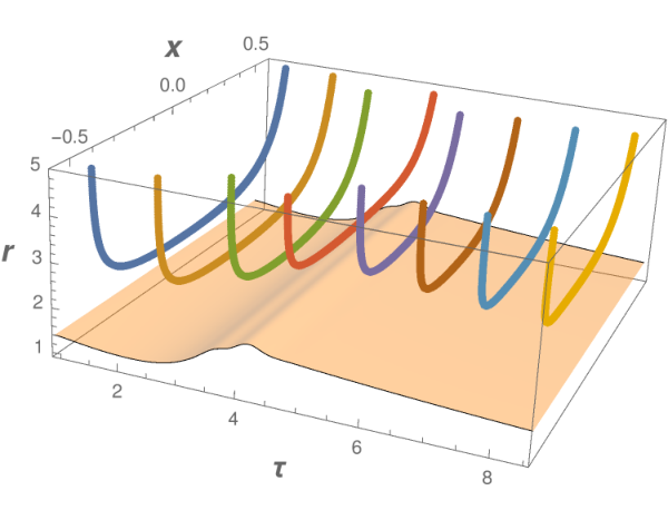
Typical resulting geodesics, obtained from the computed metric functions in (2), are depicted in Fig. 1. The thermalization of the boundary theory is studied by computing their lengths as time proceeds. The hydrodynamic expression of the geodesic lengths $\mathcal{L}_{H}$ are determined in the geometry (13)-(14) with the same regularization. This allows to define an observable by the difference $\Delta\mathcal{L}=\mathcal{L}-\mathcal{L}_{H}$.

In the case of Wilson loops as nonlocal probes of the boundary theory thermalization, we consider two shapes, circles and strips. For a Wilson loop along a circumference of radius $R=\ell/2$ on the plane $\bm{x}_{\perp}\equiv\left(x_{1},x_{2}\right)$ at the boundary, the space-like worldsheet of minimal area based on the circular path and extending in the bulk at fixed $y$ must be computed. Such a surface has an azimuthal symmetry and a tip at $\left(\tau,\bm{x}_{\perp},r\right)=\left(\tau_{*},\bm{0},r_{*}\right)$ with $\left(r_{*},\tau_{*}\right)$ input values in the calculation. The transverse section at fixed $\tau$ and $r$ is a circumference. For each section the worldsheet can be parametrized in polar coordinates $\xi^{\alpha}=(\rho,\varphi)$, so that

The area of the worldsheet is obtained from the Nambu-Goto action

with the prime in the functions $\tau$ and $r$ denoting a derivative with respect to $\rho$, and the angle $\varphi$ integrated out. Interpreting the integrand of (30) as a Lagrangian, one observes that its explicit $\rho$ dependence implies the absence of a conservation equation. The resulting Euler-Lagrange equations, although involved, can be worked out in a straightforward way. The solution $(r(\rho),\tau(\rho))$, together with the conditions (20)-(21), can be used to compute the area of the extremal surface, with the same regularization scheme adopted for the geodesic lengths. The corresponding quantity in the hydrodynamic geometry is obtained using the metric functions (14), and the probe of thermalization is given by the difference $\Delta\mathcal{A}_{C}=\mathcal{A}_{C}-\mathcal{A}_{C,H}$. Examples of extremal surfaces of circular Wilson loops, computed using the bulk geometry (2) for a particular model of quench, are depicted in Fig. 2.

A less symmetric Wilson loop is an infinite rectangular strip, regarded as a limit of an ellipsoidal loop with an elongated axis. On the boundary, we set a rectangular contour parametrized by the coordinates $\left(x_{1},x_{2}\right)$, with $-\ell/2\leq x_{1}\leq\ell/2$ and $0\leq x_{2}\leq q$. The side length $q$ is taken to infinity, and the strip is assumed to be translationally invariant along the $x_{2}$ axis. The profile of the string surface extending in the bulk at fixed $y$, having the rectangular path as its basis, is described by the embedding $\left(\tau\left(x_{1}\right),r\left(x_{1}\right)\right)$, with the conditions (22). In the following, we denote $x\equiv x_{1}$. The area of the worldsheet, in terms of the side length $q$ and a parameter $\lambda$, is given by

with $x(\lambda_{1,2})=\mp\ell/2$. Interpreting the integrand in (31) as a Lagrangian, $x$ is a cyclic variable with conjugate momentum conserved on the worldsheet. The conservation equation, using (20)-(21), reads

in terms of the coordinate $x$. Solving the equations

and

allows one to compute the area

The mentioned regularization scheme is used also for this observable. The quantity $\mathcal{A}_{RH}$ is computed in the geometry (14), and the difference $\Delta\mathcal{A}_{R}=(\mathcal{A}_{R}-\mathcal{A}_{RH})/q$ at various $\tau_{0}$ and for different $\ell$ defines an observable to study thermalization of the boundary theory. An example of rectangular Wilson loops computed in the geometry (2) is shown in Fig. 2.

We can now compute the nonlocal observables in the geometry (2), with the metric functions numerically determined in [46] for the different quench models. In the three cases, two-point correlation functions and Wilson loops, we have solved the systems of differential equations (III)-(27) and (33)-(34), together with the equations for the circular Wilson loop. The range $r\leqslant r_{0}$ is considered for the radial coordinate, with $r_{0}=12$.

References

- [1] U. W. Heinz, 9th Hadron Physics and 7th Relativistic Aspects of Nuclear Physics (HADRON-RANP 2004): A Joint Meeting on QCD and QGP Angra dos Reis, Rio de Janeiro, Brazil, March 28-April 3, 2004, AIP Conf. Proc. 739, 163 (2005), arXiv:nucl-th/0407067 [nucl-th] .
- [2] E. Shuryak, (2014), arXiv:1412.8393 [hep-ph] .
- [3] M. Ruggieri, A. Puglisi, L. Oliva, S. Plumari, F. Scardina, and V. Greco, Phys. Rev. C92, 064904 (2015), arXiv:1505.08081 [hep-ph] .
- [4] J. M. Maldacena, Int.J.Theor.Phys. 38, 1113 (1999), arXiv:hep-th/9711200 [hep-th] .
- [5] E. Witten, Adv.Theor.Math.Phys. 2, 253 (1998), arXiv:hep-th/9802150 [hep-th] .
- [6] S. Gubser, I. R. Klebanov, and A. M. Polyakov, Phys.Lett. B428, 105 (1998), arXiv:hep-th/9802109 [hep-th] .
- [7] M. Ammon and J. Erdmenger, Gauge/gravity duality (Cambridge Univ. Pr., Cambridge, UK, 2015).
- [8] J. Bjorken, Phys.Rev. D27, 140 (1983).
- [9] R. A. Janik and R. B. Peschanski, Phys.Rev. D73, 045013 (2006), arXiv:hep-th/0512162 [hep-th] .
- [10] V. E. Hubeny, S. Minwalla, and M. Rangamani, in Black holes in higher dimensions (2012) pp. 348–383, arXiv:1107.5780 [hep-th] .
- [11] Y. V. Kovchegov and A. Taliotis, Phys. Rev. C76, 014905 (2007), arXiv:0705.1234 [hep-ph] .
- [12] J. Abajo-Arrastia, J. Aparicio, and E. Lopez, JHEP 11, 149 (2010), arXiv:1006.4090 [hep-th] .
- [13] S. Bhattacharyya and S. Minwalla, JHEP 09, 034 (2009), arXiv:0904.0464 [hep-th] .
- [14] T. Albash and C. V. Johnson, New J. Phys. 13, 045017 (2011), arXiv:1008.3027 [hep-th] .
- [15] J. Aparicio and E. Lopez, JHEP 12, 082 (2011), arXiv:1109.3571 [hep-th] .
- [16] V. Keranen, E. Keski-Vakkuri, and L. Thorlacius, Phys. Rev. D85, 026005 (2012), arXiv:1110.5035 [hep-th] .
- [17] D. Galante and M. Schvellinger, JHEP 07, 096 (2012), arXiv:1205.1548 [hep-th] .
- [18] W. Baron, D. Galante, and M. Schvellinger, JHEP 03, 070 (2013), arXiv:1212.5234 [hep-th] .
- [19] E. Caceres and A. Kundu, JHEP 09, 055 (2012), arXiv:1205.2354 [hep-th] .
- [20] P. Basu and S. R. Das, JHEP 01, 103 (2012), arXiv:1109.3909 [hep-th] .
- [21] R. Auzzi, S. Elitzur, S. B. Gudnason, and E. Rabinovici, JHEP 11, 016 (2013), arXiv:1308.2132 [hep-th] .
- [22] E. Caceres, A. Kundu, J. F. Pedraza, and W. Tangarife, JHEP 01, 084 (2014), arXiv:1304.3398 [hep-th] .
- [23] H. Liu and S. J. Suh, Phys. Rev. Lett. 112, 011601 (2014a), arXiv:1305.7244 [hep-th] .
- [24] P. Basu, D. Das, S. R. Das, and K. Sengupta, JHEP 12, 070 (2013), arXiv:1308.4061 [hep-th] .
- [25] X.-X. Zeng, X.-M. Liu, and W.-B. Liu, JHEP 03, 031 (2014), arXiv:1311.0718 [hep-th] .
- [26] E. Caceres, A. Kundu, J. F. Pedraza, and D.-L. Yang, JHEP 06, 111 (2015), arXiv:1411.1744 [hep-th] .
- [27] H. Liu and S. J. Suh, Phys. Rev. D89, 066012 (2014b), arXiv:1311.1200 [hep-th] .
- [28] W. Fischler, S. Kundu, and J. F. Pedraza, JHEP 07, 021 (2014), arXiv:1311.5519 [hep-th] .
- [29] V. E. Hubeny and H. Maxfield, JHEP 03, 097 (2014), arXiv:1312.6887 [hep-th] .
- [30] M. Alishahiha, A. F. Astaneh, and M. R. M. Mozaffar, Phys. Rev. D90, 046004 (2014), arXiv:1401.2807 [hep-th] .
- [31] P. Fonda, L. Franti, V. Kernen, E. Keski-Vakkuri, L. Thorlacius, and E. Tonni, JHEP 08, 051 (2014), arXiv:1401.6088 [hep-th] .
- [32] S.-J. Zhang and E. Abdalla, Nucl. Phys. B896, 569 (2015), arXiv:1503.07700 [hep-th] .
- [33] P. M. Chesler and L. G. Yaffe, Phys.Rev.Lett. 102, 211601 (2009), arXiv:0812.2053 [hep-th] .
- [34] P. M. Chesler and L. G. Yaffe, Phys.Rev. D82, 026006 (2010), arXiv:0906.4426 [hep-th] .
- [35] P. M. Chesler and L. G. Yaffe, JHEP 1407, 086 (2014), arXiv:1309.1439 [hep-th] .
- [36] S. de Haro, S. N. Solodukhin, and K. Skenderis, Commun.Math.Phys. 217, 595 (2001), arXiv:hep-th/0002230 [hep-th] .
- [37] M. P. Heller, D. Mateos, W. van der Schee, and D. Trancanelli, Phys.Rev.Lett. 108, 191601 (2012a), arXiv:1202.0981 [hep-th] .
- [38] M. P. Heller, D. Mateos, W. van der Schee, and M. Triana, JHEP 1309, 026 (2013), arXiv:1304.5172 [hep-th] .
- [39] T. Ishii, E. Kiritsis, and C. Rosen, JHEP 08, 008 (2015), arXiv:1503.07766 [hep-th] .
- [40] J. Casalderrey-Solana, H. Liu, D. Mateos, K. Rajagopal, and U. A. Wiedemann, (2011), arXiv:1101.0618 [hep-th] .
- [41] I. Arefeva, Proceedings, 7th Conference Mathematical Methods in Physics, PoS ICMP2012, 025 (2012).
- [42] V. Balasubramanian, A. Bernamonti, J. de Boer, N. Copland, B. Craps, E. Keski-Vakkuri, B. Muller, A. Schafer, M. Shigemori, and W. Staessens, Phys. Rev. Lett. 106, 191601 (2011a), arXiv:1012.4753 [hep-th] .
- [43] V. Balasubramanian, A. Bernamonti, J. de Boer, N. Copland, B. Craps, E. Keski-Vakkuri, B. Muller, A. Schafer, M. Shigemori, and W. Staessens, Phys. Rev. D84, 026010 (2011b), arXiv:1103.2683 [hep-th] .
- [44] J. F. Pedraza, Phys. Rev. D90, 046010 (2014), arXiv:1405.1724 [hep-th] .
- [45] A. Buchel, R. C. Myers, and A. van Niekerk, JHEP 02, 017 (2015), [Erratum: JHEP07,137(2015)], arXiv:1410.6201 [hep-th] .
- [46] L. Bellantuono, P. Colangelo, F. De Fazio, and F. Giannuzzi, JHEP 07, 053 (2015), arXiv:1503.01977 [hep-ph] .
- [47] M. P. Heller and R. A. Janik, Phys.Rev. D76, 025027 (2007), arXiv:hep-th/0703243 [HEP-TH] .
- [48] R. A. Janik, Phys. Rev. Lett. 98, 022302 (2007), arXiv:hep-th/0610144 [hep-th] .
- [49] M. P. Heller, R. A. Janik, and P. Witaszczyk, Phys.Rev. D85, 126002 (2012b), arXiv:1203.0755 [hep-th] .
- [50] W. van der Schee, Phys. Rev. D87, 061901 (2013), arXiv:1211.2218 [hep-th] .
- [51] V. Balasubramanian and S. F. Ross, Phys. Rev. D61, 044007 (2000), arXiv:hep-th/9906226 [hep-th] .
- [52] J. Louko, D. Marolf, and S. F. Ross, Phys. Rev. D62, 044041 (2000), arXiv:hep-th/0002111 [hep-th] .
- [53] J. M. Maldacena, Phys. Rev. Lett. 80, 4859 (1998), arXiv:hep-th/9803002 [hep-th] .
- [54] V. E. Hubeny, Int. J. Mod. Phys. D12, 1693 (2003), arXiv:hep-th/0208047 [hep-th] .
- [55] V. E. Hubeny, JHEP 07, 093 (2012), arXiv:1203.1044 [hep-th] .
- [56] T. Hartman and J. Maldacena, JHEP 05, 014 (2013), arXiv:1303.1080 [hep-th] .
- [57] S. Caron-Huot, P. M. Chesler, and D. Teaney, Phys. Rev. D84, 026012 (2011), arXiv:1102.1073 [hep-th] .