A weakly informative prior for Bayesian dynamic model selection with applications in fMRI

Jairo A. Fúquene Patiño Affiliation: Department of Statistics, University of Warwick, UK. Brenda Betancourt Affiliation: Department of Statistical Science, Duke University, USA. João B. M. Pereira Affiliation: Instituto de Matemática, Universidade Federal do Rio de Janeiro, Brazil.

Abstract

In recent years, Bayesian statistics methods in neuroscience have been showing important advances. In particular, detection of brain signals for studying the complexity of the brain is an active area of research. Functional magnetic resonance imagining (fMRI) is an important tool to determine which parts of the brain are activated by different types of physical behavior. According to recent results there is evidence that the values of the connectivity brain signal parameters are close to zero and due to the nature of time series fMRI data with high frequency behavior, Bayesian dynamic models for identifying sparsity are indeed far-reaching. We propose a multivariate Bayesian dynamic approach for model selection and shrinkage estimation of the connectivity parameters. We describe the coupling or lead-lag between any pair of regions by using mixture priors for the connectivity parameters and propose a new weakly informative default prior for the state variances. This framework produces one-step-ahead proper posterior predictive results and induces shrinkage and robustness suitable for fMRI data in the presence of sparsity. To explore the performance of the proposed methodology we present simulation studies and an application to functional magnetic resonance imaging data.
Keywords: Dynamic Linear Models, Beta Prime Prior, Sparsity, Functional Magnetic Imaging Data.

1 Introduction

Technology in neuroscience has shown important advances over the last two decades. In particular, functional magnetic resonance imaging (fMRI) has become a powerful technique for studying the complexity of the brain and statistical analysis of this data is an active area of research (?, ? and ?). One of the objectives of analyzing fMRI data is to determine which parts of the brain are activated by different types of physical sensations or activities. The signal measured in fMRI experiments is called blood-oxygen-level dependent (BOLD) response which is a consequence of hemodynamic changes, including local changes in the blood flow, volume and oxygenation level, occurring within a few seconds of changes in neuronal activity induced by external stimuli. This underlying hemodynamic changes associated with neural activity are commonly referred to as the hemodynamic response function (HRF).

A typical BOLD response denoted by $x(t)$ , where $t$ corresponds to time, usually occurs between 3 to 10 seconds after the application of the stimulus, $s(t)$ , and reaches its peak approximately after 6 seconds [*]*Banish. To generate the BOLD signal, the stimulus function is convolved with a hemodynamic response function (HRF), denoted by $h(t)$ , as follows:

x(t)=\int_{0}^{t}h(u)s(t-u)du,

(1.1)

where $s(t)$ takes the value 1 when the stimulus is ON and 0 when the stimulus is OFF, and $u$ indexes the peristimulus time (PST) (time of neuronal firing in relation to an external stimulus). A BOLD response can be generated based on the time of the experiment, a microtime resolution and the ON/OFF sets where the role of the microtime resolution is to ensure a high precision convolution with the specific HRF. Figure 1 displays the stimulus and the respective hemodynamic response function of the experiment that we present in Section 4.

Refer to caption — Figure 1: Stimulus and hemodynamic response function of fMRI data experiment.

A common approach is to estimate the magnitude of the BOLD signal by considering a general linear model described as

y_{i,t}=\alpha_{i}+\theta_{i}x_{i,t}+\nu_{i,t},

(1.2)

where $y_{i,t}$ corresponds to the fMRI response at time $t$ at voxel $i$ (a voxel is a value on a regular grid in a three-dimensional space analogous to a pixel in a two-dimensional space), and $\nu_{i,t}$ corresponds to the measurement noise. The coefficient $\theta_{i}$ measures the “activation” at voxel $i$ and represents the magnitude of the BOLD signal at time $t$ at voxel $i$ , $x_{i,t}$ . Lastly, $\alpha_{i}$ represents the baseline trend at voxel $i$ , i.e., the base effect on the fMRI response when the effect of the BOLD signal is zero. More complex models assume that $\alpha_{i}$ varies on time representing the contribution of nuisance covariates at time $t$ , for example, periodic fluctuations due to heart rate, respiration, and head motion. Usually, a linear smoother is used to detrend the fMRI data. In equation (1.2), the “activation” coefficient $\theta_{i}$ is assumed to be invariant over time and is estimated using maximum likelihood estimation. However, research suggests this parameter may vary over time. Many studies report the detection of a strong fMRI activation in the beginning of the experiment that becomes weaker later on. Also, it is known that brain areas may interact with one another depending on the context (see ?). For these reasons, time-varying “activation” as well as the dependence between brain areas should be considered in the modeling framework. A second approach that takes both features into account, is a time-varying parameter regression which allows time-varying connectivity between two brain regions. Here, differently from what it is assumed in equation (1.2), a time series $y_{1,t}$ associated with a brain region is regressed on a time series $y_{2,t}$ associated with another brain region as follows:

	$\displaystyle y_{1,t}$	$\displaystyle=\theta_{t}y_{2,t}+\nu_{t},$		(1.3)
	$\displaystyle\theta_{t}$	$\displaystyle=\theta_{t-1}+\omega_{t},$

where $\theta_{t}$ measures the dynamic effective connectivity between the two brain regions, and $\nu_{t}$ and $\omega_{t}$ correspond to independent white noises [Buchel].

Other time-varying approaches that consider dependence among brain areas are proposed by ? and ?. Specifically, these authors explore time-varying approaches for three brain regions. To study the connectivity among them, ? proposed the following space-state model:

\displaystyle\begin{pmatrix}y_{1,t}\\ y_{2,t}\\ y_{3,t}\end{pmatrix}

\displaystyle=\begin{pmatrix}\alpha_{1}\\ \alpha_{2}\\ \alpha_{3}\end{pmatrix}+\begin{pmatrix}x_{1,t}&0&0\\ 0&x_{2,t}&0\\ 0&0&x_{3,t}\end{pmatrix}\begin{pmatrix}\theta_{1,t}\\ \theta_{2,t}\\ \theta_{3,t}\end{pmatrix}+\begin{pmatrix}\nu_{1,t}\\ \nu_{2,t}\\ \nu_{3,t}\end{pmatrix},

(1.4)

\displaystyle\begin{pmatrix}\theta_{1,t}\\ \theta_{2,t}\\ \theta_{3,t}\end{pmatrix}

\displaystyle=\begin{pmatrix}\phi_{11}x_{1,t-1}&\phi_{12}x_{2,t-1}&\phi_{13}x_{3,t-1}\\ \phi_{21}x_{1,t-1}&\phi_{22}x_{2,t-1}&\phi_{23}x_{3,t-1}\\ \phi_{31}x_{1,t-1}&\phi_{32}x_{2,t-1}&\phi_{33}x_{3,t-1}\end{pmatrix}\begin{pmatrix}\theta_{1,t-1}\\ \theta_{2,t-1}\\ \theta_{3,t-1}\end{pmatrix}+\begin{pmatrix}\omega_{1,t}\\ \omega_{2,t}\\ \omega_{3,t}\end{pmatrix},

(1.5)

where $x_{i,t}$ is the hemodynamic response function at time $t$ . The noise vectors $\boldsymbol{\omega}_{t}$ and $\boldsymbol{\nu}_{t}$ are assumed to be Gaussian and independent,

\displaystyle\boldsymbol{\omega}_{t}

\displaystyle\sim N_{3}\left(0,\begin{pmatrix}\sigma^{2}_{\omega_{1}}&0&0\\ 0&\sigma^{2}_{\omega_{2}}&0\\ 0&0&\sigma^{2}_{\omega_{3}}\end{pmatrix}\right),

\displaystyle\boldsymbol{\nu}_{t}

\displaystyle\sim N_{3}\left(0,\begin{pmatrix}\sigma^{2}_{\nu_{1}}&0&0\\ 0&\sigma^{2}_{\nu_{2}}&0\\ 0&0&\sigma^{2}_{\nu_{3}}\end{pmatrix}\right).

The model is determined by state parameters $\boldsymbol{\theta}_{t}=\left\{\theta_{1,t},\theta_{2,t},\theta_{3,t}\right\}$ linearly associated with observations $\boldsymbol{y}_{t}=\left\{y_{1,t},y_{2,t},y_{3,t}\right\}$ , respectively. Note that equation (1.4) has the same structure as equation (1.2), this equation is commonly known as the observation equation. Equation (1.5) is called the state equation and describes the dynamic of the states in a first-order vector autoregressive model conditional on the parameters, $\phi_{ij}$ , $i=1,\dots,3$ , $j=1,\dots,3$ , where $\phi_{ij}$ represent the connectivity between the brain regions $i$ and $j$ . The initial state vector $\boldsymbol{\theta}_{0}$ is assumed to follow a Normal distribution, $N_{3}(\boldsymbol{\mu}_{0},\Sigma_{0})$ , and is also assumed to be independent from the noise vectors $\boldsymbol{\omega}_{t}$ and $\boldsymbol{\nu_{t}}$ .

? use the Expectation-Maximization (EM) algorithm to estimate all the parameters of the model [Shumway]. In turn, ? extended the previous proposal using the Bayesian paradigm as well as exploring different models. In the Bayesian setting, prior information can be incorporated in the modeling and the parameters are then estimated based on both the data and the prior information. These proposals are very significant as they open the door to the use of dynamic models for investigating connectivity among brain signals. However, some questions are left unadressed. According to ? and ?, the values of the connectivity parameters are close to zero. Therefore, a natural question arises: do we need to induce some shrinkage on the activation parameters $\boldsymbol{\theta}_{t}$ and connectivity parameters $\phi_{ij}$ ? When is a connectivity parameter really equal to zero? In other words, what is the probability of having a connectivity parameter equal to zero? In addition, the authors only take into account some of the possible models for model selection purposes. In fact, in both approaches the connectivity issue is only considered as an estimation problem instead of an estimation-selection problem and we cannot conclude that the posterior estimates represent the best possible model. This leads us to the following question: how can we perform model selection over all possible models efficiently?

In this paper, the main goal is to address these questions. To this end, (i) we propose a Bayesian approach for studying the relationship among multiple brain regions by considering point-mass priors, and (ii) we induce shrinkage on both activation and connectivity parameters while capturing the high frequency behavior of fMRI data. To take this particular behavior into account, we propose a weakly informative default prior for the variances of the state parameters that correspond to the “activation” in the different brain regions. The prior induces shrinkage and robustness suitable for high frequency fMRI data with presence of sparsity, and produces one-step-ahead proper posterior predictive results. The rest of the paper proceeds as follows. Section 2 presents the formulation of the proposed methodology. Section 3 contains a simulation study using multivariate dynamic models that illustrates the performance of our modeling approach, and in Section 4 we apply the proposed methodology to functional magnetic imaging data. Finally, a short discussion is presented in Section 5.

2 Modeling Approach

Model selection has been one of the most active research areas in Bayesian analysis in recent years. Mixture priors have been used in various settings as a variable selection-estimation tool in regression models (see for example ?, ? and ?). On the other hand, ? use point-mass priors on the roots of the autoregressive polynomial model to handle model uncertainty and unit roots in autoregressive models. ? use point-mass priors for model selection to analyze DNA microarray data. Among the most important and recent suggested approaches for model selection, we find the horseshoe prior by ?, which arises from considering a half-Cauchy distribution for the scale parameter of a Normal prior. ? propose to use Inverted-Gamma densities for the scale parameter in a hierarchical fashion, and thus obtain a hypergeometric family for modelling a dynamic autoregressive model.

In this work, we propose a Bayesian approach for studying the dynamic relationship between multiple brain regions. We describe the coupling or lead-lag relationships between any pair of regions using point-mass mixture priors for the connectivity parameters as follows:

\displaystyle\phi_{ij}\sim\pi N(0,\sigma^{2}_{ij})+(1-\pi)\delta_{0}(\phi_{ij}),

(2.1)

such that the connectivity parameter is a non-zero drawn from the Normal prior with zero mean and variance $\sigma_{ij}^{2}=1/\tau_{ij}$ with probability $\pi$ , and zero with probability $1-\pi$ . An advantage of this prior is that hypothesis testing and model selection can be performed at the same time. In contrast to the approach of ?, one important feature of the point-mass prior approach is that the assumption that connectivity parameters are equal to zero for some brain regions is not necessary. The point-mass priors allow us to compute the posterior probability of having a connectivity parameter equal to zero in a simple fashion. In other words, with the point-mass approach we can not only obtain posterior inference on the connectivity parameters, but also consider all possible models for model comparison purposes.

2.1 Prior elicitation for the connectivity parameters

In this section, we show the prior elicitation and corresponding simulation of the connectivity parameters. We consider this same elicitation in both the simulation and application sections. We utilize prior information from results of the brain imaging data applications presented in ?, and use the proposal of ? to elicit the connectivity parameters. Following ?, we choose to find the $\text{Gamma}(c,d)$ prior for the precision $\tau_{ij}=1/\sigma^{2}_{ij}$ by eliciting information about the first percentile of the sampling distribution. We assume a prior with mean zero and cumulative probability equal to 0.01 at -1 leading to $\tau_{0}\equiv(-1/\Phi^{-1}(0.01))^{-2}\approx 1.82$ . By equating $\tau_{0}=(c-1)/d$ or equivalently $c=\tau_{0}d+1$ , the prior for the precision parameter of the point-mass prior is $\tau_{ij}\sim\text{Gamma}(3.78,1.53)$ .

In order to specify the prior for the parameter $\pi$ of the point-mass prior, we use information from the results in ?. In their application, the number of 9 connectivity parameters different from zero is equal to 6. Therefore, we assume $\pi\sim\text{Beta}(a,b)$ with $a_{\pi}=6$ and $b_{\pi}=3$ , so that the corresponding prior mean and standard deviation are $E(\pi)=0.66$ and $\sqrt{V(\pi)}=0.149$ , respectively. Figure 2 displays the Normal prior for the point-mass prior, the corresponding variance and the weights using the elicitation described above.

2.2 A weakly informative default prior for the state variances

Weakly informative default prior choices for variances have been proposed in the past for Bayesian hierarchical models. For example, ? considers half-t prior distributions for scale parameters in hierarchical models. The author proposes this weakly informative default prior to replace the very sensitive Inverse-Gamma $(\epsilon,\epsilon)$ “non-informative” conjugate prior in order to have a limiting posterior distribution for hierarchical models.

We now present our proposal of a new weakly informative default prior for the state variances in the general framework of Bayesian dynamic linear models (BDLM). The hierarchical definition of a BDLM for $t=1,\dots,T$ is,

$\displaystyle y_{t}\|\boldsymbol{\theta}_{t}$	$\displaystyle\sim N(F_{t}\boldsymbol{\theta}_{t},V_{t}),$	(2.2)
$\displaystyle\boldsymbol{\theta}_{t}\|\boldsymbol{\theta}_{t-1}$	$\displaystyle\sim N(G_{t}\boldsymbol{\theta}_{t-1},V_{t}W_{t}),$
$\displaystyle\boldsymbol{\theta}_{t-1}\|y_{1:t-1}$	$\displaystyle\sim N(m_{t-1},C_{t-1}),$

where $\boldsymbol{\theta}_{t}$ corresponds to a vector of states of dimension $p$ varying smoothly over time and $F_{t}$ and $G_{t}$ are matrices of dimension $m\times p$ and $p\times p$ , respectively. The parameter $V_{t}$ is the variance of the observation $y_{t}\mid\boldsymbol{\theta}_{t}$ and $V_{t}W_{t}$ is the variance of the state parameter $\boldsymbol{\theta}_{t}\mid\boldsymbol{\theta}_{t-1}$ . In turn, $m_{t}$ and $C_{t}$ correspond to the posterior mean and posterior variance of the state parameter $\theta_{t}$ given $y_{1:t-1}$ . For simplicity, we let $y_{t}$ be the value of an univariate time series at time $t$ with $\theta_{t}$ corresponding to an unobservable state vector. Also, we consider $F_{t}=1$ , $G_{t}=G=\phi$ , $V_{t}=V=\sigma^{2}$ and $W_{t}=\tau^{2}_{t}$ . The model (2.2) is studied in the seminal book of ?, where it is assumed that the state variance $W_{t}$ is unknown and discount factors are proposed for modelling it.

Let us consider the one-step-ahead predictive distribution of $y_{t}$ given $y_{1:t-1}$ for the model in (2.2), which follows a Gaussian distribution with mean and variance given by

	$\displaystyle f_{t}$	$\displaystyle=m_{t-1},$
	$\displaystyle Q_{t}$	$\displaystyle=C_{t-1}+\sigma^{2}+\tau^{2}_{t}\sigma^{2}.$

Assume $\sigma^{2(*)}=C_{t-1}+\sigma^{2}$ and $\sigma^{2}=1$ for simplicity. Then the density function of the one-step-ahead predictive distribution is as follows:

\displaystyle p(y_{t}|y_{1:t-1},\sigma^{2(*)},\lambda_{\theta}^{-1})\propto\dfrac{1}{\sqrt{\sigma^{2(*)}+\lambda_{\theta}^{-1}}}\exp\left\{-\frac{1}{2}\dfrac{(y_{t}-m_{t-1})^{2}}{\sigma^{2(*)}+\tau^{2}_{t}}\right\}.

(2.3)

where $\lambda_{\theta}=1/(\tau^{2}_{t}\sigma^{2})$ is the state precision. The Jeffreys prior $p(\sigma^{2(*)})\propto\sigma^{-2(*)}$ poses no issues. However, analogously to ?, in the hierarchial model case if we consider the Jeffreys prior $p(\tau^{2}_{t})\propto\tau^{-2}_{t}$ , we have that the density function in (2.3) is positive at $\tau^{2}_{t}=0$ and therefore $p(\tau^{2}_{t})$ fails to be integrable at the origin. Also, the conjugate Inverse-Gamma $(\epsilon,\epsilon)$ prior is very sensitive to choices of very small values of $\epsilon$ leading to an improper posterior one-step-ahead predictive density.

On the other hand, the Beta prime density has been considered by different authors as a default prior for variances in Bayesian model selection (see ? and ?), hierarchical models [polson], and for modelling outliers and structural breaks in BDLMs [fuquenep]. The Beta prime density with shape parameters $p$ and $q$ and scale dynamic parameter $\beta_{t}$ is described as,

\pi(\tau^{2}_{t})=\frac{\Gamma(p+q)}{\Gamma(p)\Gamma(q)}\frac{1}{\beta_{t}}\frac{\left(\dfrac{\tau^{2}_{t}}{\beta_{t}}\right)^{p-1}}{\left(1+\dfrac{\tau^{2}_{t}}{\beta_{t}}\right)^{p+q}},\;\;\;\;\tau>0,

(2.4)

where $\Gamma(\cdot)$ corresponds to the gamma function. Here, for mathematical properties and computational simplicity, we propose the use of a Beta prime density with $p=1$ and $q=(\upsilon_{t}-1)/2$ :

p(\tau^{2}_{t})\propto\left(1+\dfrac{\tau^{2}_{t}}{\beta_{t}}\right)^{-(\upsilon_{t}+1)/2}.

(2.5)

Combining the density (2.3) and the prior (2.5), we have that $p(y_{t}|y_{1:t-1},\sigma^{2(*)},\lambda_{\theta}^{-1})$ is defined when $\tau^{2}_{t}\rightarrow 0$ . For the case $\tau^{2}_{t}\rightarrow\infty$ , the exponential term in (2.3) is less than or equal to 1. For the remaining term, we have that $(1+\tau^{2}_{t}/\sigma^{2(*)})^{-1/2}(1+\tau^{2}_{t}/\beta_{t})^{-(\upsilon_{t}+1)/2}$ is integrable and hence $p(y_{t}|y_{1:t-1},\sigma^{2(*)},\lambda_{\theta}^{-1})$ is proper.

The Beta prime distributions considered here induce one-step-ahead proper posterior predictive results and sampling from these priors is straightforward due to the mixing Gamma property $\tau^{2}_{t}\sim\text{Gamma}(1,\beta_{t}/\rho_{t})$ and $\rho_{t}\sim\text{Gamma}((\upsilon_{t}-1)/2,1)$ . Also, by definition, the Beta prime for the scale parameter $\lambda_{\theta}=\tau^{-2}_{t}$ has shape parameters $p=(\upsilon_{t}-1)/2$ and $q=1$ and a dynamic scale parameter $1/\beta_{t}$ . The priors for the observation and state variances are summarized in the display below. To make the inference procedure feasible, we use Monte Carlo Markov Chain (MCMC) methods. The summary of the algorithm is available in Appendix A of the supplementary materials.

$\displaystyle V_{t}^{-1}$	$\displaystyle=1/\sigma^{2}=\lambda_{y},\quad p(\sigma^{2})\propto 1/\sigma^{2},$	(2.6)
$\displaystyle W_{t,i}^{-1}$	$\displaystyle=\lambda_{y}\lambda_{\theta,i}\omega_{\theta,t_{i}},\quad i=1,\dots,p$
$\displaystyle\omega_{\theta,t_{i}}\|\nu_{\theta,t_{i}}$	$\displaystyle\sim\text{Gamma}(\nu_{t_{i}}/2,\nu_{t_{i}}/2),$
$\displaystyle\lambda_{\theta,i}$	$\displaystyle\sim\text{Gamma}((\nu_{t_{i}}-1)/2,\rho_{t_{i}}/\beta_{t_{i}}),$
$\displaystyle\rho_{t_{i}}$	$\displaystyle\sim\text{Gamma}(1,1),$
$\displaystyle\beta_{t_{i}}$	$\displaystyle\sim\text{Gamma}(1,\xi_{t,i}),$
$\displaystyle\xi_{t,i}$	$\displaystyle\sim\text{Gamma}(1,1),$
$\displaystyle\upsilon_{\theta,t_{i}}$	$\displaystyle\sim\text{Multinomial}(1,\varphi_{i}),$
$\displaystyle\varphi_{i}$	$\displaystyle\sim\text{Dirichlet}(\alpha_{i}),$

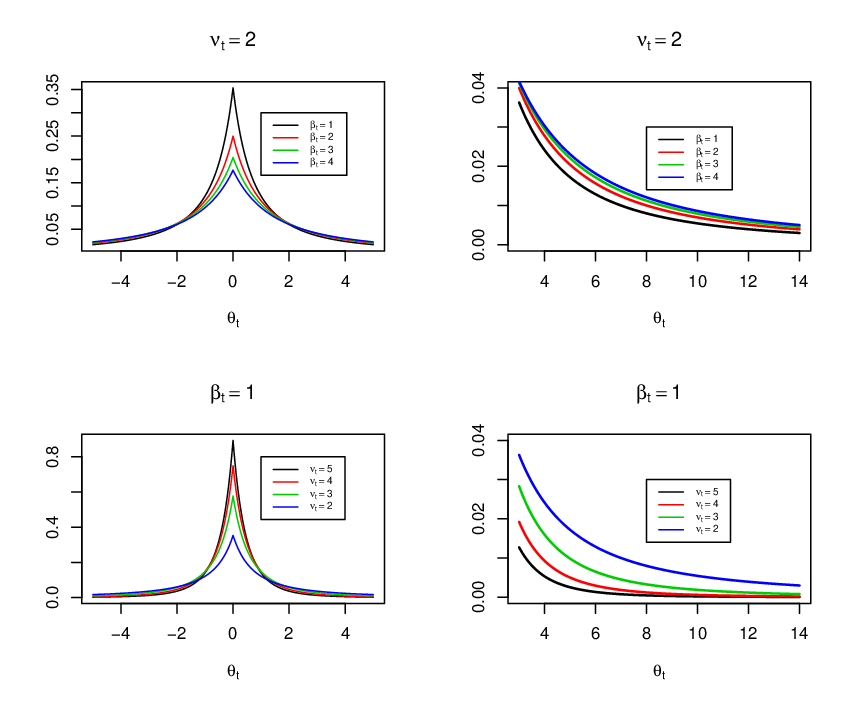
Under this formulation, the state variances follow a Student’s t-distribution with $\nu_{t}$ degrees of freedom by assuming $\tau_{t}^{2}|\lambda_{\theta,i},\omega_{\theta,t_{i}}\sim N(0,\sigma^{2}(\lambda_{\theta,i}\omega_{\theta,t_{i}})^{-1})$ , where the degrees of freedom follow a multinomial distribution as assumed by ?. The marginal prior for the states can be found in a closed form as follows: (see proof in Appendix B - supplementary material )

Proposition 2.1.

The marginal prior of the states in model 2.2 using the variance formulation in 2.5 is as follows:

\displaystyle\pi(\theta_{t}|G_{t}\theta_{t-1},\sigma,\nu_{t},\beta_{t})

\displaystyle=\dfrac{\nu_{t}-1}{2\sqrt{\sigma\nu_{t}\beta_{t}}\left(1+\dfrac{|\theta_{t}-G_{t}\theta_{t-1}|}{\sqrt{\sigma\nu_{t}\beta_{t}}}\right)^{\nu_{t}}}.

(2.7)

Particular cases of priors as the one in equation (2.7) have appeared repeatedly in the literature over the years under various names (Linnik, Meridian, double-Pareto, generalized t and normal- gamma), e.g. ?, ?, ?, ? and ?. Also, the particular case when $\sigma=\nu_{t}=G_{t}=1$ , corresponds to the Scaled-Beta-Cauchy prior proposed by ?. The $g$ -prior used in ? seems to be in the same class, except that the prior for $\tau^{2}_{t}$ is improper. Figure 3 illustrates how the density is more heavy-tailed when the degrees of freedom $\nu_{t}$ increases, the marginal prior becomes weakly informative and the variance increases with $\beta_{t}$ . Moreover, to avoid over-shrinking of the states and to learn fully automatically, we also introduce priors for the parameters in equation (2.5).

Note that shrinkage is also induced for the connectivity parameters $\phi$ , where a marginal prior with a similar form to the one in (2.7) could be obtained by using the full conditional distribution of $\phi$ and integrating out the state variances. Also, when $\nu_{t}\rightarrow\infty$ , the prior becomes more similar to a Normal prior in the first level of the hierarchical model, although with a Student’s t tail behavior. Therefore, the novelty of our approach is not only proposing a default state variance prior suitable for detecting sparse state-signals of BDLMs applied to fMRI data. We also induce shrinkage in the estimation of the autoregressive coefficient parameter.

We present now synthetic examples to illustrate the performance of our proposed weakly informative prior. We consider the following BDLM:

\displaystyle y_{t}

\displaystyle=\theta_{t}+v_{t},

\displaystyle\theta_{t}

\displaystyle=\phi\theta_{t-1}+w_{t},

(2.8)

where the sparse signals $w_{t}$ , $t=1,\dots,T$ , follow a two component Normal mixture model given by

w_{t}\sim\pi N(0,V)+(1-\pi)N(0,\kappa W),

(2.9)

and $v_{t}\sim N(0,V)$ . We consider $\kappa=20$ , $\phi=0.5$ , $W/V=\{1,0.6,0.2\}$ and $\pi=0.9$ . The Markov Chain Monte Carlo scheme, where we also use the Forward Filtering Backward Sampling (FFBS) algorithm proposed in ? for posterior inference purposes is presented in Appendix A - supplementary material. We reached convergence of all parameters in 5,000 iterations after a burn-in period of 2,000 iterations with a thinning period of 10. We spent approximately 50 minutes to obtain the results using the ? program and a PC with Intel(R) Xeon(R) 2.80 GHZ and 4 GB RAM. Figures 4 to 6 illustrate the results. In the right panels, the red circles correspond to values from the $N(0,\kappa V)$ mixture component and the black circles correspond to values from the $N(0,W)$ component. We can see in all cases that the posterior distributions of $1/\lambda_{y}$ and $1/\lambda_{\theta,i}$ reproduce the true parameters. The posterior mean density of $\phi$ represents nicely the true value and the corresponding probability in all cases. The posterior mean of the state variances $W_{t}=1/(\lambda_{y}\lambda_{\theta,i}\omega_{\theta,t})$ and the posterior mean of the latent parameters $\omega_{\theta,t}$ properly identify the sparse state signals with values $\omega_{\theta,t}<1$ . The Figures illustrate how shrinkage is induced under the small values of the $\phi$ parameter.

3 Simulation study

We explore two different modeling settings on simulated data. We first fitted a model where the state precisions, $\lambda_{\theta,i}$ , are fixed. In the second model we consider the precisions $\lambda_{\theta,i}$ unknown and we use the proposed weakly informative prior for the state variances presented in the last section. For both settings, we consider three time series of size $T=285$ and we use different values of the signal/noise ratio $\lambda_{\theta,i}^{-1}/\lambda_{y,i}^{-1}=\left\{0.5,1,2\right\}$ and $\lambda_{\theta,i}^{-1}=1$ in order to study the performance of a model with sparse state parameters. The model and parameter values used in the simulation (also applied in the last section) are the following follows:

	$\displaystyle\small\boldsymbol{y}_{t}=\begin{pmatrix}y_{t,1}\\ y_{t,2}\\ y_{t,3}\end{pmatrix},\hskip 9.24994pt\boldsymbol{F}_{t}=\begin{pmatrix}1&0&0&x_{t,1}&0&0\\ 0&1&0&0&x_{t,1}&0\\ 0&0&1&0&0&x_{t,1}\end{pmatrix},$
	$\displaystyle\boldsymbol{G}_{t}=\begin{pmatrix}1&0&0&0&0&0\\ 0&1&0&0&0&0\\ 0&0&1&0&0&0\\ 0&0&0&\phi_{11}x_{t-1,1}&\phi_{12}x_{t-1,2}&\phi_{13}x_{t-1,3}\\ 0&0&0&\phi_{21}x_{t-1,1}&\phi_{22}x_{t-1,2}&\phi_{23}x_{t-1,3}\\ 0&0&0&\phi_{31}x_{t-1,1}&\phi_{32}x_{t-1,2}&\phi_{33}x_{t-1,3}\\ \end{pmatrix},$

	$\displaystyle\boldsymbol{V}_{t}$	$\displaystyle=\boldsymbol{V}=diag\begin{pmatrix}\lambda_{y,1}^{-1},&\lambda_{y,2}^{-1},&,\lambda_{y,3}^{-1}\end{pmatrix},$
	$\displaystyle\boldsymbol{W_{t}}$	$\displaystyle=\boldsymbol{W}=diag\begin{pmatrix}0,0,0,(\lambda_{y,1}\lambda_{\theta,1})^{-1},&(\lambda_{y,2}\lambda_{\theta,2})^{-1},&,(\lambda_{y,3}\lambda_{\theta,3})^{-1}\end{pmatrix},$
	$\displaystyle\boldsymbol{\theta}_{t}^{{}^{\prime}}$	$\displaystyle=\begin{pmatrix}\alpha_{1},&\alpha_{2},&\alpha_{3},&\theta_{t,1},&\theta_{t,2},&\theta_{t,3}\end{pmatrix}.$

Table 1 displays the values of the connectivity parameters used to simulate the data. These values are based on the results of ? where some connectivity regions are close to zero.

Table 1: True values for the connectivity regions in the simulation study.

$\phi_{11}$	$\phi_{12}$	$\phi_{13}$	$\phi_{21}$	$\phi_{22}$	$\phi_{23}$	$\phi_{31}$	$\phi_{32}$	$\phi_{33}$
0	-0.1495	-3.0382	0	-0.8365	-0.2667	0.4179	0.1365	0

We use a non-informative Gamma prior for the observational precisions with hyperparameters $a_{y,i}=0.001$ and $b_{y,i}=0.001$ , and a Beta $(a_{\pi},b_{\pi})$ prior for the weights $\pi$ with hyperparameters $a_{\pi}=6$ and $b_{\pi}=3$ . We assume the weakly informative default prior for the state precisions. For the connectivity parameters $\phi_{ij}$ , we consider the point-mass prior with the elicitation presented in Section 2. Using standard methods such as the autocorrelation function, time series traces and cumulative estimates of the quantiles, we verified the convergence of all parameters using a burn-in period of 10000 iterations with 30000 subsequent iterations to generate the estimated posterior distributions (see MCMC scheme in Appendix A - supplementary material). To have a measure of the forecasting accuracy, we use two common criteria called the mean absolute deviation (MAD) and the mean square error (MSE), which are defined as

\displaystyle MAD

\displaystyle=\frac{1}{285}\sum_{i=1}^{3}\sum_{t=1}^{T}|e_{i,t}|

\displaystyle MSE

\displaystyle=\frac{1}{285}\sum_{i=1}^{3}\sum_{t=1}^{T}e_{i,t}^{2},

where $e_{i,t}=y_{i,t}-(\alpha_{i}^{s}+F^{{}^{\prime}}_{t}\theta^{s}_{i,t})$ , for $\alpha_{i}^{s}$ and $\theta^{s}_{i,t}$ , the simulated parameters.

Table 2: Forecasting accuracy measures for two models settings where

\lambda_{\theta,i}

is considered known or unknown. The data was simulated using

\lambda_{\theta,i}=1

Signal/noise ratio	MAD	MSE
$\lambda_{\theta,i}^{-1}/\lambda_{y,i}^{-1}=0.5$ ; $\lambda_{\theta,i}$ unknown	4.370	3.458
$\lambda_{\theta,i}^{-1}/\lambda_{y,i}^{-1}=0.5$ ; $\lambda_{\theta,i}$ known	4.010	3.184
$\lambda_{\theta,i}^{-1}/\lambda_{y,i}^{-1}=1$ ; $\lambda_{\theta,i}$ unknown	2.403	1.904
$\lambda_{\theta,i}^{-1}/\lambda_{y,i}^{-1}=1$ ; $\lambda_{\theta,i}$ known	2.752	2.185
$\lambda_{\theta,i}^{-1}/\lambda_{y,i}^{-1}=2$ ; $\lambda_{\theta,i}$ unknown	1.736	1.374
$\lambda_{\theta,i}^{-1}/\lambda_{y,i}^{-1}=2$ ; $\lambda_{\theta,i}$ known	1.812	1.431

Table 2 shows the results of the measures of accuracy in the simulation. We are interested in comparing MAD and MSE for the same model when the state precisions are known or unknown in order to evaluate the performance of the proposed weakly informative prior. According to the results, using the proposed weakly informative prior for the state precisions could be a good choice given that the MAD and MSE values are similar to those obtained when the precisions are known for the different signal/noise ratios. In Appendix C - supplementary material, in Figures 1, 5, 9, 13, 17 and 21, we can see how most of the values of the posterior means for the connectivity parameters are close to the true values. We can also see in Figures 2, 3, 6, 7, 10, 11, 14, 15, 18, 19, 22 and 23 that the posterior densities of trends, state and observational variances are concentrated around the true values. Similarly, according to Figures 4, 8, 12, 16, 20 and 24 the true state parameters are generally within the 95% simulated credible intervals.

4 Application: fMRI data

This section presents the application of the proposed methodology for researching the mechanism of attentional control with fMRI time series from a single subject. We consider the same example shown in ? and ?, who consider state-space models for studying the dynamic relationship between multiple brain regions. According to ?, three systems involve attentional control: (1) the task-relevant process system, which involves the task-relevant stimulus dimension; (2) the task-irrelevant processing system, which allows to process the task-irrelevant stimulus dimension; and (3) a source of control that develops the top-down selection bias, which may increase the neural activity within the task-relevant processing system and/or may suppress the neural activity within the task irrelevant processing system. Many applications have found the dorsal prefrontal cortex to be a main source of the attention control.

4.1 Experimental design

Data acquisition. A GE Signa magnetic resonance imaging system equipped for echoplanar imaging (EPI) was used for data acquisition (see ?). Eleven right-handed native English-speaking participants (7 men and 4 women, ranging in age from 18 to 30) were included in the study. For each run, a total of 300 EPI images were acquired (TR = 1517 ms, TE = 40 ms, flip angle $90^{\circ}$ ), each consisting of 15 contiguous slices (thickness 7 mm, in-plane resolution 3.75 mm), parallel to the AC-PC line. A high-resolution 3D anatomical set (T1-weighted three-dimensional spoiled-gradient echo images) was collected for each participant, as well as T1 weighted images of our functional acquisition slices. The head coil was fitted with a bite bar to minimize head motion during the session. Stimuli were presented on a goggle system designed by Magnetic Resonance Technologies. In the experiment, two phases were explored:

•

Learning phase. The subject learned to associate each of three unfamiliar shapes with one of three color words (i.e. “BLUE”, “YELLOW” or “GREEN”) and at the end of this phase it was verified that participants could correctly provide the name of the three shapes with 100% accuracy. Next, the shapes were presented in white without their associated words, one at the time in random order. Finally, the participants were instructed to practice naming each shape subvocally with its corresponding word. Each shape was presented a total of 32 times.
•

Test phase. In this phase, blue, yellow and green ink colors were used and two types of trials were presented:
- –
  
  The interference trial. In the interference trial the shape was printed in an ink color incongruent with the color used to name the shape.
- –
  
  The neutral trial. In the neutral trial the shape was printed in white, which was not a color name for any of the shapes.

A block design was used where the block of neutral trials was alternated with the block of interference trials. We have 6 blocks of neutral and interference trials, where each block consists of 18 trials presented at a rate of one trial each 2 seconds. Each trial consisted of a 300 milliseconds fixation cross by a 1,200 millisecond presentation of the stimulus (shape) and a 500 millisecond inter-trial interval. Finally, participants were instructed to subvocally name each shape with the corresponding color from the learning phase ignoring the ink color in which the shape was presented. Subvocalization (characterized by the occurrence in the mind of words in speech order with or without inaudible articulation of the speech organs) was utilized in an effort to avoid possible motion artifacts. Figure 1 displays the stimulus and hemodynamic response function of this experiment.

4.2 The three regions of interest

We are interested in the attention control network that reflects the brain’s ability to discriminate between relevant and irrelevant information in tasks that require a certain level of concentration. The lingual gyrus, the middle occipital gyrus and the dorsolateral prefrontal cortex were selected. The lingual gyrus (LG) is a visual area sensitive to color information which can be used as a site for processing task-irrelevant information (i.e., the ink color [*]*kelley). The middle occipital gyrus (MOG) is also a visual area sensitive to shape information and it represents a site for processing task-relevant information (i.e., the shapes form). The dorsolateral prefrontal cortex (DLPFC) is selected to represent the source of attentional control. Figure 7 displays the standardized time series of the three regions of interest. The three time series regions were detrended using a linear smoother which is roughly a linear regression fitted to the $k$ -nearest neighbors of a given point and it is used to predict the response at that point.

We consider the same multivariate dynamic model presented in Section 3 where the three regions are the lingual gyrus (LG), the middle occipital gyrus (MOG), and the dorsolateral prefrontal cortex (DLPFC), respectively. For instance, $\phi_{11}$ represents the self-feedback in the LG region, and $\phi_{12}$ characterizes the coupling relationship between the LG and MOG regions. In the MCMC algorithm, we obtained convergence of all parameters using 30000 iterations after a burn-in period of 10000 iterations and a thin of 4 where different initial values were considered. We used a non-informative Gamma prior for the observational precisions with hyperparameters $a_{y,i}=0.001$ and $b_{y,i}=0.001$ . The state variances are modeled using the proposed weakly informative prior. For the connectivity parameters, we considered the point-mass prior with the elicitation presented in section 2.1 for the precision and the weights.

Table 3: Posterior Mean, posterior standard deviation and posterior probability of

\phi_{ij}=0

Parameter	Posterior mean	Posterior SD	$P(\phi_{ij}=0\|\text{data})$
$\phi_{11}$	0	0	1.00
$\phi_{12}$	-0.0335	0.09	0.99
$\phi_{13}$	-5.4126	0.64	0.00
$\phi_{21}$	0	0	1.00
$\phi_{22}$	0.0308	0.01	0.99
$\phi_{23}$	-4.940	0.71	0.00
$\phi_{31}$	-0.091	0.05	0.99
$\phi_{32}$	-0.1250	0.06	0.98
$\phi_{33}$	0.3221	0.18	0.61

Table 3 shows the posterior summary for the connectivity parameters. Figures 8 to 10 display the results obtained using the proposed Bayesian approach. Our approach indicates that the probability of the regions DLFCP and LG or DLFCP and MG being connected is high ( $P(\phi_{13}\neq 0|\text{data})=P(\phi_{23}\neq 0|\text{data})=1$ ). Also, with probability equal to 0.61, the posterior mean of $\phi_{33}$ is different from zero. Therefore, there is evidence of a positive self-feedback at DLFCP. On the other hand, there was not self-feedback in the two sites of control, LG and MOG, ( $P(\phi_{11}=0|\text{data})=1$ and $P(\phi_{22}=0|\text{data})=0.99$ ). Because of the posterior probability $P(\phi_{31}=0|\text{data})=0.99$ and $P(\phi_{32}=0|\text{data})=0.98$ , we cannot conclude that there is any influence on the MOG from the LG and DLFCP regions. Our results showed that there was not substantial suppression from MOG on LG ( $P(\phi_{12}=0|\text{data})=0.99$ ) and also from LG on MOG ( $P(\phi_{21}=0|\text{data})=1$ ). The results are consistent with ?, and the connectivity between the regions is consistent with the theory of attentional control.

5 Discussion

To model the connectivity between brain signals for a particular subject, we propose a multivariate dynamic Bayesian model that addresses the main limitations of previous approaches to this problem. The introduction of a point-mass prior for the connectivity parameters allows us to perform automatic model selection over the set of all possible models. Our proposal also includes a new weakly informative default variance state prior that is suitable for modelling the high frequency behavior characteristic of fMRI data. This prior induces robustness and shrinkage for the sparse state signals leading to more coherent inference for the connectivity parameters. We showed that the proposed model works in a large number of distinct scenarios where different signal/noise ratio values are considered. Finally, when the proposed approach was applied to fMRI data for a particular subject for static connectivity parameters over time, we obtained accurate results in accordance with the theory of attentional control.

Acknowledgements

We thank Moon-Ho Ringo Ho for his help in the preparation of the fMRI data.

References

[2] [] Armagan, D., Dunson, D. & Lee, J. (2010), Bayesian generalized double pareto shrinkage, in ‘Technical report, Duke University Department of Statistical Science’.
[4] [] Banich, M. T., Milhan, M., Atchley, R., Cohen, N. J., Webb, N. J., Wszalek, A., Kramer, T., Liang, A. F., Wright, Z. P., Shenker, A. & Margin, R. (2000), ‘fMRI studies of stroop tasks reveal unique roles of anterior and posterior brain systems in attentional selection’, Journal Conective Neuroscience 12, 988–1000.
[6] [] Bhattacharya, S., Ho, M. R. & Purkayastha, S. (2006), ‘A Bayesian approach to modeling dynamic effective connectivity with fMRI data’, NeuroImage 30, 794–812.
[8] [] Buchel, C. & Friston, K. (1998), ‘Dynamic changes in effectivity connectivity characterized by variable parameter regression and Kalman filtering’, Neuroimagine 12, 366–380.
[10] [] Carvalho, C. M., Polson, N. G. & Scott, J. G. (2010), ‘The horseshoe estimator for sparse signals’, Biometrika 97, 465–480.
[12] [] Christensen, R., Jhonson, W., Branscum, A. & Hanson, T. (2011), Bayesian ideas and data analysis, Chapman and Hall.
[14] [] Clyde, M. & George, E. I. (2004), ‘Model uncertainty’, Statistical Science 19, 81–94.
[16] [] Devroye, L. (1996), ‘Random variate generation in one line of code’, J. Charnes, D. Morrice, D. Brunner, and J. Swain, editors, Proceedings of the 1996 Winter Simulation Conference pp. 275–272.
[18] [] Friston, K. J. & Price, C. J. (2001), ‘Dynamic representations and generative models of brain function’, Brain Research Bulletin 54, 275ñ285.
[20] [] Fruwirth-Schnatter, S. (1994), ‘Data augmentation and dynamic linear models’, Journal of Time Series Analysis 15, 183–202.
[22] [] Fúquene, J. A., Perez, M. E. & Pericchi, L. R. (2014), ‘An alternative to the Inverted Gamma for the variances to modelling outliers and structural breaks in dynamic models’, Brazilian Journal of probability and statistics 28-2, 288–299.
[24] [] Gelman, A. (2006), ‘Prior distributions for variance parameters in hierarchical models’, Bayesian Anaysis 3, 515–533.
[26] [] George, E. I. & McCulloch, R. E. (1993), ‘Variable selection via Gibbs Sampling’, Journal of the American Statistical Association 88, 881–889.
[28] [] Griffin, J. & Brown, P. (1996), ‘Inference with normal-gamma prior distributions in regression problems’, Bayesian Analysis 5(1), 171–188.
[30] [] Huerta, G. & West, W. (1999), ‘Priors and component structures in autoregressive time series models’, Journal Royal Statistics B-61, 881–899.
[32] [] Kawata, T. (1972), Fourier Analysis in Probability Theory, Academic Press.
[34] [] Kelley, W. M., Miezin, F. M., McDermmott, K., Buckner, R. L., Raichle, M. E., Cohen, N. J., Ollinger, J. M., Akbudak, E., Conturo, T. E., Snyder, A. Z. & Peterson, S. E. (1998), ‘Hemispheric specialization in human dorsal frontal cortex and medial temporal lobe for verbal and nonverbal memory encoding’, Neuron 20, 927–936.
[36] [] Lazar, N. A. (2008), The Statistical Analysis of Functional MRI Data, Vol. 1, Springer.
[38] [] Lazar, N. A., Eddy, W. F., Genovese, C. R. & Welling, J. (2001), ‘Statistical issues in fMRI for brain imaging’, International Statistical Review p. 105ñ127.
[40] [] Lee, F., Caron, A., Doucet & Holmes., C. (2011), Bayesian sparsity-path-analysis of genetic association signal using generalized t priors., in ‘Technical report, University of Oxford, http://arxiv.org/abs/1106.0322, 2011’.
[42] [] Liang, F., Paulo, R., Molina, G., Clyde, M. A. & Berger, J. (2008), ‘Mixture of g priors for Bayesian Variable Selection’, Journal of the American Statistical Association 103, 410–423.
[44] [] Madigan, A. E. D. & Hoeting, J. A. (1997), ‘Bayesian model averaging for linear regression models’, Journal of the American Statistical Association 92, 1197–1208.
[46] [] Milham, M., Banich, M. & Cohen, N. (2003), ‘Practice-related effects demonstrate complementary role of anterior cingulate and prefrontal cortices in attentional control’, Neuroimagine 18, 483–493.
[48] [] Petris, G., Petrone, S. & Campagnoli, P. (2010), Dynamic linear models with R, Springer-Verlag.
[50] [] Polson, N. G. & Scott, J. (2012a), ‘Good, great or lucky? Screening for firms with sustained superior performance using heavy-tailed priors’, The annals of applied statistics 6, 161–185.
[52] [] Polson, N. G. & Scott, J. (2012b), ‘On the half-Cauchy prior for a global scale parameter’, Bayesian Anaysis 7, 1–16.
[54] [] R Development Core Team (2015), R: A Language and Environment for Statistical Computing, R Foundation for Statistical Computing, Vienna, Austria. ISBN 3-900051-07-0.
*#1
[56] [] Ringo-Ho, M. H., Ombao, H. & Shumway, R. (2005), ‘A state-space approach to modelling brain dynamics’, Statistica Sinica 15, 407–425.
[58] [] Scott, J. & Berger, J. O. (2006), ‘An exploration of aspects of Bayesian multiple testing’, Journal statistical planning and inference 136, 2144–2162.
[60] [] Shumway, R. H. & Stoffer, D. S. (2011), Time series analysis and its applications, Springer.
[62] [] Steel, M. & Ley, E. (2012), ‘Model of g-priors for Bayesian model averaging with economic applications’, Journal of Econometrics 171, 251–266.
[64] [] West, M. (1984), ‘Outliers models and prior distributions in bayesian linear regression’, Journal of the Royal Statistics Society. Series B. 46-3, 431–439.