Horizon as Critical Phenomenon

The AdS/CFT correspondence[1, 2, 3] opened the door to address questions on gravity from the perspectives of quantum field theory. However, it is often difficult to make concrete progress in this direction because one usually does not have a full control on both sides of the duality. In order to take full advantage of the duality, it is desired to have a first principle construction of holographic duals from field theories, which may allow one to pose certain questions on gravity in solvable field theories.

The general link between boundary field theories and bulk gravitational theories is made through renormalization group (RG), where the bulk variables are scale dependent couplings and the radial direction corresponds to a length scale[4, 5, 6]. However, the RG suggested by holography is different from the Wilsonian RG in that the bulk equation of motion for the single-trace couplings captures the flow of multi-trace operators as well[7, 8]. Furthermore, the bulk variables have intrinsic quantum fluctuations while the Wilsonian RG is deterministic. This hints that one has to promote the Wilsonian RG to quantum RG to make a precise connection with holography.

Quantum RG provides a prescription to construct holographic duals for general field theories[9, 10, 11]. In quantum renormalization group, RG flow is described as a dynamical system, where couplings of field theories are promoted to quantum operators. While only a subset of operators are kept, quantum fluctuations of their couplings capture other operators that are not explicitly included in the RG flow. The fluctuations in RG path make the bulk theory quantum mechanical. The bulk theory that governs the dynamical RG flow includes gravity because the metric that sources the energy-momentum tensor is also promoted to dynamical variable[10, 11].

The goal of this paper is to provide some insight into horizon by applying quantum RG to a solvable field theory. We will show that horizons can be understood as critical phenomena, where scale dependent couplings exhibit a non-analyticity as a critical RG scale is approached. A divergent length scale associated with spread of entanglement at the critical point gives rise to the divergent red shift at the horizon. We demonstrate this by deriving the bulk geometry for a solvable field theory from quantum RG. For earlier ideas on possible connections between black hole horizons and phase transitions, see [12] and references there-in.

Here is an outline and the main results of the paper. In section II, we explain how quantum states can be defined from actions of field theories. This is different from the usual connection between a $D$-dimensional action and a $(D-1)$-dimensional quantum state. Here, an action itself is promoted to a wave function, and a $D$-dimensional action defines a $D$-dimensional quantum state. Then the partition function is written as an overlap between two quantum states, called IR and UV states. If the IR state is chosen to be a fixed point, the UV state is constructed from deformations turned on in a given field theory. As deformations in the Wilsonian effective action are renormalized under the conventional RG flow, the UV quantum state evolves under quantum RG flow. The full theory with the deformations may or may not flow to the IR fixed point depending on the kind and strength of the deformations.

In section III, we explain that RG flow can be viewed as a wave function collapse where the UV state is gradually projected toward the IR state. In section IV, we show that the wave function collapse is described by the radial evolution of a holographic dual via quantum RG, and that the quantum Hamiltonian that generates the RG flow can be faithfully represented in basis states constructed from actions which include only single-trace operators. In doing so, we also explain the structure of tensor network in the bulk. The tensor network generated from quantum RG has no pre-imposed kinematic locality. Instead, the bulk space is made of a network of multi-local tensors of all sizes. Dynamical locality in bulk is determined by action principle which controls the strength of non-local tensors.

In section V, we apply quantum RG to the U(N) vector model, which was previously studied numerically [13]. In this paper, we obtain the analytic solution for the bulk equations of motion in the large $N$ limit. The exact solution allows one to derive the bulk metric from the first principle construction. For this, a real space coarse graining is employed. The IR fixed point is chosen to be a direct product state in the insulating phase, and the kinetic (hopping) terms are regarded as deformation to the fixed point. The Hamiltonian that generates coarse graining gradually removes entanglement in the UV state. When the theory with the deformation is still in the insulating phase, the UV state is smoothly projected to the direct product state. In this case, the bulk geometry is capped off at a finite proper distance in the radial direction. The proper distance in the radial direction measures the depth of RG transformations that is necessary to remove entanglement entirely in the UV state. This confirms the conjecture[14] that relates the radial distance in the bulk and complexity. When the deformation is large that the system is no longer in the insulating phase, the UV state can not be smoothly projected to the direct product state as entanglement in the UV state keeps spreading out to larger length scales under the RG flow. The persistent entanglement gives rise to the extended geometry with an infinite proper distance in the radial direction. The obstruction to smooth projection culminates in a non-analyticity of the scale dependent state caused by the divergent length scale in the spread of entanglement. This can be viewed as dynamical critical behavior[15, 16] as the quantum RG flow for Euclidean field theories is interpreted as a Hamiltonian flow under an imaginary time evolution. The critical point gives rise to the Poincare horizon in the anti-de Sitter (AdS) space or the Lifshitz geometry in the bulk, depending on whether the chemical potential is turned on or off. In sections VI and VII, we conclude with summary and comments on universality of horizon and possible way to extend to Lorentzian space.

Before we move on to the main body of the paper, we provide an intuitive picture of quantum RG with emphasis on the differences from other approaches.

• •

  Wilsonian RG and Quantum RG :

  An action is specified by the sources (couplings) for operators allowed within a theory. The conventional Wilsonian RG describes the evolution of the sources under a coarse graining. The Wilsonian RG flow is classical because the sources at low energy scales are determined without any uncertainty from the sources specified at high energy scales. Beta functions, which are first order differential equations, govern the flow of the classical sources. If the complete set of sources are kept within the flow, the Wilsonian RG is exact. However, it is usually difficult to keep all sources, especially for strongly coupled theories where there is no obvious way of truncating operators without knowing the spectrum of scaling dimensions beforehand.

  Quantum RG is an alternative exact scheme which keeps only a subset of operators (single-trace operators). It is based on the observation that a theory with arbitrary operators can be represented as a linear superposition of theories which include only single-trace operators. In other words, one can keep the exact information about an action with arbitrary sources in terms of a quantum wave function defined in the space of the single-trace sources. For example, the Boltzmann weight of a theory with operators, $O$, $O^{2}$, $O^{3}$, … can be represented as a linear superposition of the theories which have only $O$ through $e^{J_{1}O+J_{2}O^{2}+J_{3}O^{3}+...}=\int dj_{1}~\Psi(j_{1})e^{j_{1}O}$, where the wave function $\Psi(j_{1})$ is chosen such that the original action which is non-linear in $O$ is reproduced upon integrating over $j_{1}$. This reduces to the standard Hubbard-Stratonovich transformation when the cubic and higher order terms are absent. Then the exact RG flow generated from a coarse graining naturally becomes a quantum evolution of the wave function because an action at any scale can be represented as a wave function. The information on the infinite number of classical sources is kept by the wave function of one source, by taking advantage of the linear superposition principle. In this sense, what quantum RG is to the conventional RG is what quantum computer is to the classical computer.

  The advantage of quantum RG is that one can keep only single-trace operators, which is typically a much smaller set compared with the full set of operators. However, quantum RG is not necessarily simpler than the conventional RG for general theories because one has to include quantum fluctuations of the single-trace sources. The simplification arises when quantum fluctuations in RG paths are small in the presence of a large number of degrees of freedom. For this reason, quantum RG can be most useful in studying strongly interacting theories with large numbers of degrees of freedom.

• •

  Tensor networks and Quantum RG :

  In quantum RG, the partition function is expressed as a path integration of dynamical sources defined in one higher dimensional space, where the extra dimension corresponds to the RG scale. The path integral represents the sum over RG paths defined in the space of single-trace sources. The resulting path integral can be identified as a tensor network where the bulk action becomes the constituent tensors that need to be contracted through path integral. There are some characteristics of the tensor network generated from quantum RG, which distinguish it from other forms of tensor networks. First, the bulk tensor network that arises in quantum RG has no pre-imposed locality. This is due to the fact that the set of single-trace operators in general include non-local operators. The examples include the Wilson-loop operators in gauge theories and the bi-local operators in vector models. For this reason, the bulk space described by quantum RG is not only quantum but also non-local in general. A classical and local geometry emerges only in a class of systems, where quantum fluctuations of the dynamical sources are small, and the sources for non-local operators decay fast enough at the saddle point. Therefore, the degree of locality in the bulk is a dynamical feature rather than a choice of local tensor structure put in by hand. Second, quantum RG chooses the dynamical sources and their conjugate momenta as internal variables that are contracted (integrated over) in the bulk. Because the source for the energy-momentum is the metric, the quantum RG naturally gives a bulk theory which includes dynamical gravity. Although one may define a notion of distance for any local tensor network, it generally does not represents a dynamical space if the connectivity of the network is rigid.

We consider a partition function in $D$-dimensional Euclidean space,

$\displaystyle Z=\int D\phi~e^{-S},$

(1)

where $\phi$ represents the fundamental field of the theory and $S$ is the action. If the $D$-dimensional partition function originates from a $(D-1)$-dimensional quantum theory, the path integral sums over spacetime trajectories in the Euclidean time. On the other hand, the Boltzmann weight itself can be viewed as a $D$-dimensional wave function. From an action $S$, one can define a quantum state

$\displaystyle\big|S\big>$

$\displaystyle=$

$\displaystyle\int D\phi~e^{-S[\phi]}\big|\phi\big>,$

(2)

where $\big|\phi\big>$ is a complete set of basis states which form a Hilbert space with the norm,

$\displaystyle\big<\phi^{{}^{\prime}}\big|\phi\big>=\prod_{i,a}\delta(\phi^{{}^{\prime}}_{ia}-\phi_{ia}).$

(3)

Here $i$ is an index for the $D$-dimensional space, and $a$ represents internal flavour(s). For concreteness, one can use a lattice regularization for the $D$-dimensional space. From the point of view of the original $(D-1)$-dimensional quantum theory, Eq. (2) represents a state of spacetime path.

Any quantity that can be defined for usual quantum states can be defined for the states generated from actions. For example, the von Neumann entanglement entropy can be defined for the $D$-dimensional states as it is defined for the $(D-1)$-dimensional state for the original quantum system. However, the physical meanings of the two objects are somewhat different. The $D$-dimensional state encodes entanglement between (Euclidean) spacetime events rather than entanglement between the bits that reside in the $(D-1)$-dimensional space.

An action can be written as

$\displaystyle S=-\sum_{i}J_{i}O_{i}-\sum_{i,j}J_{ij}O_{i,j}+...,$

(4)

where $O_{i_{1},i_{2},..,i_{n}}$’s are operators that depends on $n$ space coordinates, and $J_{i_{1},i_{2},..,i_{n}}$’s are the sources. For notational simplicity, we suppress the indices for internal flavours. One can identify the Boltzmann weight associated with a $n$-point operator as a rank $(n+1)$ tensor,

$\displaystyle T^{J}_{\phi_{i_{1}},\phi_{i_{2}},..,\phi_{i_{n}}}=e^{JO_{i_{1},i_{2},..,i_{n}}}.$

(5)

Here one of the indices in the tensor is the source, $J$, and the remaining indices are the values of the fields at $n$ points, $\phi_{i_{1}}$, $\phi_{i_{2}}$,..,$\phi_{i_{n}}$. The indices are in general continuous. The $D$-dimensional state is then written as

$\displaystyle\big|S\big>$

$\displaystyle=$

$\displaystyle\int D\phi~\Psi_{J}[\phi]\big|\phi\big>,$

(6)

where the wave function is given by a direct product of the multi-local tensors,

$\displaystyle\Psi_{J}[\phi]$

$\displaystyle=$

$\displaystyle\prod_{n}\prod_{i_{1},..,i_{n}}T^{J_{i_{1},i_{2},..,i_{n}}}_{\phi_{i_{1}},\phi_{i_{2}},..,\phi_{i_{n}}}.$

(7)

It is noted that $\Psi_{J}[\phi]$ is a wave function of $\phi$. The sources are variational parameters in the wave function. These are illustrated in Fig. 1. For local actions, the sources for multi-local operators decay exponentially as the separation between coordinates increases. States generated from local actions are called local states.

If there is a symmetry in the action, $S[\phi]$ is invariant under the symmetry transformations,

$\displaystyle S[U_{s}\phi]=S[\phi].$

(8)

Here $U_{s}$ is a matrix that acts on $\phi$ which is viewed as a giant vector, where space points and internal indices form the vector index. The corresponding quantum state $\big|S\big>$ is invariant under a unitary transformation $\hat{U}_{s}$ which acts on the basis states as

$\displaystyle\hat{U}_{s}\big|\phi\big>=\big|U_{s}\phi\big>.$

(9)

We call states generated from symmetric actions symmetric states. The set of symmetric states form symmetric Hilbert space.

A symmetric action can be written as a sum of singlet operators with sources,

$\displaystyle S$

$\displaystyle=$

$\displaystyle-{\cal J}^{M}{\cal O}_{M}.$

(10)

Here $\{{\cal O}_{M}\}$ represents a complete set of singlet operators that are invariant under the symmetry of the theory. Here $M$, which is summed over, denotes not only different types of operator, but also operators at different positions in $D$ dimensions. In general, ${\cal O}_{M}$ can be multi-local operators that depend on multiple coordinates. In matrix models, for example, a trace of matrix fields at multiple positions and product of them form singlet operators. ${\cal J}^{M}$ are the sources. Now symmetric states can be labeled by the sources of the singlet operators,

$\displaystyle\big|\{{\cal J}\}\big>$

$\displaystyle=$

$\displaystyle\int D\phi~e^{{\cal J}^{M}{\cal O}_{M}}\big|\phi\big>.$

(11)

However, these states form an over-complete basis of the symmetric Hilbert space. There is a smaller set of complete basis. The minimal set of operators that span the full symmetric Hilbert space are called single-trace operators, $\{O_{n}\}$. In large $N$ matrix models, they are the operators that involve one trace. But the definition of single-trace operator can be extended to any theory. In general, $\{O_{n}\}$ is defined to be the minimal set of singlet operators of which all singlet operators can be expressed as polynomials[11],

$\displaystyle{\cal O}_{M}=\sum c^{n_{1},n_{2},..}_{M}O_{n_{1}}O_{n_{2}}..$

(12)

The single-trace operators span the full symmetric Hilbert space because

	$\displaystyle\big|S\big>$	$\displaystyle=$	$\displaystyle\int D\phi~e^{\sum_{k}{\cal J}^{n_{1},n_{2},..,n_{k}}O_{n_{1}}O_{n_{2}}..O_{n_{k}}}~\big|\phi\big>$		(13)
		$\displaystyle=$	$\displaystyle\int DjD\phi~e^{-j^{n}(j_{n}^{*}-O_{n})+\sum_{k}{\cal J}^{n_{1},n_{2},..,n_{k}}j_{n_{1}}^{*}j_{n_{2}}^{*}..j_{n_{k}}^{*}}~\big|\phi\big>.$

Here $Dj\equiv\prod_{n}dj^{n}dj_{n}^{*}$. $j^{n},j_{n}^{*}$ are auxiliary fields introduced for each single-trace operator, where $j_{n}^{*}$ is the complex conjugate of $j^{n}$. We used the identity $f(O)=\frac{1}{\pi}\int dj~dj^{*}~e^{-j(j^{*}-O)}~f(j^{*})$[9]. A multiplicative constant that is independent of sources is ignored in Eq. (13). Eq. (13) shows that any singlet state can be written as a linear superposition of the states constructed from the single-trace operators as

$\displaystyle\big|S\big>$

$\displaystyle=$

$\displaystyle\int Dj~\Psi_{S}(j)~\big|j\big>,$

(14)

where

$\displaystyle\big|j\big>$

$\displaystyle=$

$\displaystyle\int D\phi~e^{j^{n}O_{n}}\big|\phi\big>$

(15)

is the complete single-trace basis and

$\displaystyle\Psi_{S}(j)$

$\displaystyle=$

$\displaystyle e^{-j_{n}^{*}j^{n}+\sum_{k}{\cal J}^{n_{1},n_{2},..,n_{k}}j_{n_{1}}^{*}j_{n_{2}}^{*}..j_{n_{k}}^{*}}$

(16)

is the wave function written in the space of $j$. Graphically, symmetric states are made of single-trace tensors whose sources are contracted with the tensor given by $\Psi_{S}(j)$ (Fig. 2).

Therefore it is natural to associate an action of a field theory with a wave function. Instead of specifying classical sources for all singlet operators, one can specify a quantum wave function defined in the space of the single-trace sources. The quantum RG is based on the fact that the exact Wilsonian RG flow defined in the classical space of full singlet operators can be faithfully represented as a quantum evolution of wave function defined in the space of single-trace operators[11]. In the following section, we will first show that RG flow can be viewed as a collapse of such wave function defined from an action.

The goal of renormalization group is to integrate out degrees of freedom partially, and examine how the action for the remaining degrees of freedom flow. The order in which the degrees of freedom are integrated out is determined by a reference action $S_{0}$. It is convenient to choose $S_{0}$ to be a fixed point of the theory in order to keep the reference action invariant under the scale transformation. If $S_{0}$ is chosen to be the free kinetic term as is usually done in perturbative RG, the order of integration is organized according to momentum. However, there is freedom to choose different reference action. Once the choice is made for the reference action, the remaining action, $S_{1}=S-S_{0}$ is regarded as a deformation to the reference action.

Now we define quantum states associated with the reference action and the deformation in a given field theory as

	$\displaystyle\big|S_{0}^{*}\big>$	$\displaystyle=$	$\displaystyle\int D\phi~e^{-S_{0}^{*}[\phi]}\big|\phi\big>,$
	$\displaystyle\big|S_{1}\big>$	$\displaystyle=$	$\displaystyle\int D\phi~e^{-S_{1}[\phi]}\big|\phi\big>.$		(17)

$\big|S_{0}^{*}\big>$ and $\big|S_{1}\big>$ are called IR and UV states respectively. The reason why we define the IR state from the complex conjugate of the reference action is because the partition function for the full action $S=S_{0}+S_{1}$ is given by the overlap between the two states,

$\displaystyle Z=\big<S_{0}^{*}\big|S_{1}\big>.$

(18)

If $\big|S_{0}^{*}\big>$ and $\big|S_{1}\big>$ are written in the single-trace basis, $\big|S_{0}^{*}\big>=\int Dj^{{}^{\prime}}~\Psi_{0}(j^{{}^{\prime}})\big|j^{{}^{\prime}}\big>$, $\big|S_{1}\big>=\int Dj~\Psi_{1}(j)\big|j\big>$, the partition function becomes

$\displaystyle Z$

$\displaystyle=$

$\displaystyle\int Dj^{{}^{\prime}}Dj~\Psi^{*}_{0}(j^{{}^{\prime}})\big<j^{{}^{\prime}}\big|j\big>\Psi_{1}(j).$

(19)

This is illustrated in Fig. 3.

A coarse graining procedure in the renormalization group transformation can be viewed as a collapse of the UV state towards the IR state. To illustrate the idea, let us begin with a simple example of one real scalar integration,

$\displaystyle Z=\int d\phi~e^{-S_{0}-S_{1}}.$

(20)

Here $S_{0}=\frac{m^{2}}{2}\phi^{2}$ is the quadratic reference action. All the higher order terms are included in the deformation $S_{1}[\phi]$. In the presence of the $Z_{2}$ symmetry, $\phi\rightarrow-\phi$, only even powers are allowed in the action. For coarse graining, one adds an auxiliary field $\Phi$ with a mass $\mu$. The physical field and the auxiliary field are mixed into a new basis, $\phi=\phi^{{}^{\prime}}+\Phi^{{}^{\prime}}$, $\Phi=\frac{m}{\mu\sqrt{2dz}}(-2dz\phi^{{}^{\prime}}+\Phi^{{}^{\prime}})$, in which the new action becomes

$\displaystyle S=\frac{m^{2}e^{2dz}}{2}\phi^{{}^{\prime}2}+\frac{m^{2}}{4dz}\Phi^{{}^{\prime}2}+S_{1}[\phi^{{}^{\prime}}+\Phi^{{}^{\prime}}].$

(21)

The fluctuations of $\phi^{{}^{\prime}}$ are slightly suppressed compared to the original field $\phi$ due to the slightly increased mass. The missing fluctuations are carried by $\Phi^{{}^{\prime}}$. Therefore, integrating out $\Phi^{{}^{\prime}}$ has the effect of partially including fluctuations of $\phi$. It generates quantum corrections,

$\displaystyle\delta_{1}S_{1}$

$\displaystyle=$

$\displaystyle\frac{dz}{m^{2}}\left[\frac{\partial^{2}S_{1}}{\partial\phi^{{}^{\prime}2}}-\left(\frac{\partial S_{1}}{\partial\phi^{{}^{\prime}}}\right)^{2}\right].$

(22)

Rescaling of the field, $\phi^{{}^{\prime}}=e^{-dz}\phi^{{}^{\prime\prime}}$, brings $S_{0}$ back to the original form, and generates an additional correction from $S_{1}$,

$\displaystyle\delta_{2}S_{1}$

$\displaystyle=$

$\displaystyle-dz\phi^{{}^{\prime\prime}}~\frac{\partial S_{1}}{\partial\phi^{{}^{\prime\prime}}}.$

(23)

The relation between the original field $\phi$ and the low energy field $\phi^{{}^{\prime\prime}}$ is given by

$\displaystyle\phi^{{}^{\prime\prime}}=e^{-dz}\left(\phi-\frac{\mu}{m}\sqrt{2dz}\Phi\right).$

(24)

Renaming $\phi^{{}^{\prime\prime}}$ to $\phi$, we note that the net quantum correction to $S_{1}$ is generated by a quantum evolution,

$\displaystyle e^{-(S_{1}+\delta_{1}S_{1}+\delta_{2}S_{1})}=\big<\phi\big|e^{-dz\hat{H}}\big|S_{1}\big>,$

(25)

where $\big|S_{1}\big>=\int d\phi~e^{-S_{1}[\phi]}\big|\phi\big>$ is the quantum state corresponding to the action $S_{1}$, and

$\displaystyle\hat{H}=\frac{1}{m^{2}}\hat{\pi}^{2}+i\hat{\phi}\hat{\pi}$

(26)

is the Hamiltonian. $\hat{\phi}$ has eigenvalue $\phi$ for $\big|\phi\big>$, $\hat{\phi}\big|\phi\big>=\phi\big|\phi\big>$. $\hat{\pi}$ is the conjugate momentum that obeys the commutation relation, $[\hat{\phi},\hat{\pi}]=i$.

Here $\hat{H}$ is the generator of the renormalization group transformation. Although $\hat{H}$ is not a Hermitian Hamiltonian, it is symmetric under the combined transformation of the parity (P), $\phi\rightarrow-\phi,\pi\rightarrow-\pi$ and the time reversal (T), $\phi\rightarrow\phi,\pi\rightarrow-\pi,i\rightarrow-i$. The PT-symmetry guarantees that both $\hat{H}$ and $\hat{H}^{\dagger}$ have real eigenvalues[17]. However, $\hat{H}$ and $\hat{H}^{\dagger}$ have different eigenstates which are related to each other through a similarity transformation. The ground state wave function of $\hat{H}^{\dagger}$ ($\hat{H}$) is $e^{-S_{0}}$ ($1$) with the ground state energy $0$. Since $\hat{H}^{\dagger}$ annihilates $\big|S_{0}^{*}\big>=\big|S_{0}\big>$, the IR state is invariant under the transformation, which reflects the fact that $S_{0}$ is a fixed point. Therefore, the partition function is invariant under the insertion of $e^{-dz\hat{H}}$. On the other hand, $e^{-dz\hat{H}}$ acting on $\big|S_{1}\big>$ generates a non-trivial evolution of the deformation,

$\displaystyle Z=\big<S_{0}^{*}\big|S_{1}\big>=\big<S_{0}^{*}\big|e^{-dz\hat{H}}\big|S_{1}\big>=\big<S_{0}^{*}\big|S_{1}+\delta S_{1}\big>.$

(27)

Now an infinite sequence of $e^{-dz\hat{H}}$ is inserted to write

$\displaystyle Z=\lim_{z\rightarrow\infty}\big<S_{0}^{*}\big|e^{-z\hat{H}}\big|S_{1}\big>.$

(28)

Since $\hat{H}$ has the unique ground state with a finite gap in the spectrum, $\big|S_{1}\big>$ is gradually projected toward the ground state in the long time limit, where we interpret $z$ as an imaginary time. The process of projecting the state $\big|S_{1}\big>$ to the ground state is the RG flow. In the large $z$ limit, $e^{-z\hat{H}}\big|S_{1}\big>$ approaches the ground state of $\hat{H}$, which has a trivial overlap with $\big|S_{0}^{*}\big>$. The information on the partition function is encoded in the norm of the projected state.

In the above example, the RG flow is smooth. Any state with a finite number of degrees of freedom is smoothly projected to the ground state. However, this is not true in the thermodynamic limit because the large system size limit and the large RG time limit do not commute in general. As will be discussed in Sec. V, $\big|S_{1}\big>$ can not be smoothly projected to the ground state in the thermodynamic limit if the deformation is large that the system is no longer in the phase described by the assumed IR fixed point described by $S_{0}$.

Here let us consider another simple example to relate RG flow with wave function collapse. We consider a $D$-dimensional scalar field theory, where the reference action is chosen to be the free kinetic term,

$\displaystyle S_{0}=\frac{1}{2}\int d^{D}k~G^{-1}_{\Lambda}(k)\phi_{k}\phi_{-k}.$

(29)

Here $k$ is momentum, and $G^{-1}_{\Lambda}(k)$ is a regularized kinetic term with UV cut-off $\Lambda$, e.g., $G^{-1}_{\Lambda}(k)=e^{\frac{k^{2}}{\Lambda^{2}}}k^{2}$. All the interactions are included in the deformation, $S_{1}[\phi]$. After lowering the cut-off $\Lambda\rightarrow\Lambda e^{-dz}$ followed by a rescaling of field and momentum, $\phi_{k}\rightarrow e^{\frac{D+2}{2}dz}\phi_{e^{dz}k}$, one obtains a quantum correction $\delta S_{1}$[18]. The quantum correction can be generated by

$\displaystyle e^{-(S_{1}[\phi]+\delta S_{1}[\phi])}=\big<\phi\big|e^{-dz\hat{H}}\big|S_{1}\big>,$

(30)

where

$\displaystyle\hat{H}=\int dk\left[\frac{\tilde{G}(k)}{2}\hat{\pi}_{k}\hat{\pi}_{-k}-i\left(\frac{D+2}{2}\hat{\phi}_{k}+k\partial_{k}\hat{\phi}_{k}\right)\hat{\pi}_{-k}\right]$

(31)

with $\tilde{G}(k)=\frac{\partial G_{\Lambda}(k)}{\partial\ln\Lambda}$. The conjugate momentum obeys the commutation relation, $[\phi_{k},\pi_{k^{\prime}}]=i\delta(k+k^{{}^{\prime}})$. The first term in Eq. (31) is from lowering $\Lambda$, and the second term originates from the rescaling of field and momentum. However, the validity of Eq. (27) is subtle in this case because $\big|S_{0}\big>$ is not exactly annihilated by $\hat{H}^{\dagger}$ in general. Upon applying $\hat{H}^{\dagger}$ to $\big|S_{0}\big>$, one is left with a total derivative term, $-\frac{1}{2}\int d^{D}k~\nabla_{k}\cdot(\vec{k}G^{-1}\phi_{k}\phi_{-k})$. This is due to the fact that the range of momentum changes as momentum is relabeled. The total derivative term can be dropped if the range of momentum is formally taken to infinity. However, the partition function is not finite in this case. To avoid this subtlety, we will adopt a real space renormalization group scheme in the following. Another advantage of using a real space RG scheme is the easiness in implementing a local RG[19, 10, 11, 20] by choosing the speed of coarse graining differently at different points in space.

In the real space renormalization group scheme, we can choose $\big|S_{0}^{*}\big>$ to be a direct product state. Accordingly, the Hamiltonian of which $\big|S_{0}^{*}\big>$ is the ground state (with zero energy) is ultra-local,

$\displaystyle\hat{H}=\sum_{i}\alpha_{i}\hat{h}_{i},$

(32)

where $\hat{h}_{i}$ is the on-site term of the Hamiltonian, and $\alpha_{i}$ is a local speed of coarse graining. We note that the choice of $\hat{h}_{i}$ is not unique for a given $\big|S_{0}\big>$. Different Hamiltonians project excited states in different rates, which corresponds to use different RG scheme. Furthermore, one can choose any $\alpha_{i}>0$ because $\big|S_{0}^{*}\big>$ is a direct product state. Here we will choose a gauge $\alpha_{i}=1$ for simplicity. The partition function is given by

$\displaystyle Z=\int Dj^{(0)}~\big<S_{0}^{*}\big|j^{(0)}\big>\Psi(j^{(0)}),$

(33)

where $\Psi(j^{(0)})$ is the wave function associated with the UV state as is illustrated in Fig. 4.

Since $\big|S_{0}^{*}\big>$ is annihilated by $\hat{H}^{\dagger}$, the overlap is invariant under the insertion of $U=e^{-dz\hat{H}}$ (Fig. 5 (a)),

$\displaystyle Z=\int Dj^{(0)}~\big<S_{0}^{*}\big|e^{-dz\hat{H}}\big|j^{(0)}\big>\Psi(j^{(0)}).$

(34)

Even though $\big|j^{(0)}\big>$ includes only single-trace tensors, the evolution generates multi-trace tensors,

$\displaystyle e^{-dz\hat{H}}\big|j^{(0)}\big>=\int D\phi~~e^{j^{(0)n}O_{n}-dzC^{n_{1},n_{2},..}[j^{(0)}]\left(O_{n_{1}}O_{n_{2}}...\right)}\big|\phi\big>.$

(35)

Furthermore, longer-range tensors are generated from short-range tensors. The sources for the longer-range tensors and multi-trace tensors are functions of $j^{(0)}$ as is illustrated in Fig. 5 (b).

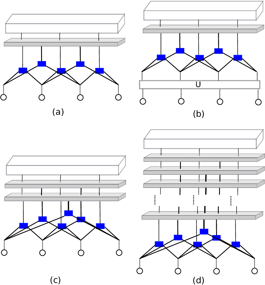
Because general symmetric states can be represented as a linear combination of $\big|j\big>$, the Hamiltonian should have a faithful representation in the space of $j$. The state with multi-trace operators can be again written as a linear combination of the single-trace states,

$\displaystyle e^{-dz\hat{H}}\big|j^{(0)}\big>=\int Dj^{(1)}~~e^{-j^{*(1)}_{n}(j^{(1)n}-j^{(0)n})-dzC^{n_{1},n_{2},..}[j^{(0)}]\left(j^{*(1)}_{n_{1}}j^{*(1)}_{n_{2}}...\right)}\big|j^{(1)}\big>.$

In Fig. 6(a), the gray box represents the tensor, $e^{-j^{*(1)}_{n}(j^{(1)n}-j^{(0)n})-dzC^{n_{1},n_{2},..}[j^{(0)}]\left(j^{*(1)}_{n_{1}}j^{*(1)}_{n_{2}}...\right)}$, whose external legs are $j^{(0)}$ and $j^{(1)}$. By applying this successively, the partition function can be written as a path integration of auxiliary sources $j^{(n)}$ introduced at $n$-th step of coarse graining. This is illustrated in Fig. 6 (b)-(d). In the continuum ($dz\rightarrow 0$) limit, one obtains

	$\displaystyle Z$	$\displaystyle=$	$\displaystyle\lim_{z\rightarrow\infty}\big<S_{0}^{*}\big|e^{-z\hat{H}}\big|S_{1}\big>,$		(37)
		$\displaystyle=$	$\displaystyle\int Dj(z)~~\big<S_{0}^{*}\big|j(\infty)\big>~e^{-\int_{0}^{\infty}dz\left(j_{n}^{*}\partial_{z}j^{n}+{\cal H}[j^{*},j]\right)}\Psi(j(0)).$

${\cal H}[j^{*},j]$ is the coherent state representation of the quantum Hamiltonian,

$\displaystyle\hat{\cal H}[j^{\dagger},j]$

$\displaystyle=$

$\displaystyle\left(j^{\dagger}_{n_{1}}j^{\dagger}_{n_{2}}...\right)C^{n_{1},n_{2},..}[j].$

(38)

$j^{n}$, $j_{n}^{\dagger}$ are quantum operators defined in the space of single-trace operators. The space of single-trace operators depends on the type of field theory. For gauge theories, it is the space of loops[9]. For vector models, it is the space of bi-local coordinates[13]. The operators satisfy the commutation relation $[j^{n},j_{m}^{\dagger}]=\delta^{n}_{m}$. $j_{n}^{\dagger}$ ($j^{n}$) creates (annihilates) a closed string in gauge theories, and a bi-local object in vector models. Because the complete set of single-trace operators include extended objects, the bulk theory is kinematically non-local. $\hat{\cal H}$ describes quantum evolution of those extended objects in the bulk.

The Hamiltonian gradually projects the generally entangled UV state to the direct product state. The bulk theory can be viewed as a process of removing entanglement present in the UV state. For other approaches of entanglement based renormalization group, see Refs. [21, 22, 23, 24]. In the present case, the disentangler $e^{-z\hat{H}}$ is a non-unitary operator. On the other hand, we can not choose any local operator to remove short-distance entanglement. The Hamiltonian should annihilate the reference state in order to keep the overlap invariant.

Since $\hat{H}$ is an ultra-local Hamiltonian given by sum of on-site terms, ${\cal H}$ has an important property. If one expands $C^{n_{1},n_{2},..}[j]$ in power series of $j$ as

$\displaystyle C^{n_{1},n_{2},..}[j]=\sum_{m_{1},m_{2},..}~f^{n_{1},n_{2},..}_{m_{1},m_{2},..}~j^{m_{1}}j^{m_{2}}..,$

(39)

the ultra-locality implies that $f^{n_{1},n_{2},..}_{m_{1},m_{2},..}$ is non-zero only if for every site $i$ included in the support of $\{n_{k}\}$ there exists some $m_{l}$ whose support includes $i$. In other words, $\hat{\cal H}$ can create an object $n$ by $j_{n}^{\dagger}$ only when there are pre-existing objects whose support include the support of $n$. This restriction can be understood as arising from a local symmetry that is present in the Hamiltonian[9]. We will illustrate this point further in the next section through a concrete example.

The path integral in Eq. (37) is nothing but contractions of tensors that form a network in the bulk as is illustrated in Fig. 6. The internal variables contracted in the bulk are the dynamical sources. In the large $N$ limit, quantum fluctuations are suppressed, and the contractions of tensors are dominated by the saddle-point[10]. The tensor network generated from quantum RG has some differences from other forms of tensor networks[25, 26, 27, 28, 22, 29, 30], some of which have been proposed for holography. The tensor network described in Eq. (37) has no pre-imposed kinematic locality in the bulk because one has to include tensors associated with multi-local single-trace operators of all sizes. This kinematic non-locality is crucial in order to have a sense of diffeomorphism invariance in the bulk[13, 31]. In the absence of kinematic locality in the bulk, the degree of locality in the classical geometry that emerges in the large $N$ limit is determined dynamically. In this sense, locality in the bulk is a dynamical feature of the theory rather than a pre-imposed structure built in the tensor network.

As a concrete application, we consider the $D$-dimensional vector model,

$\displaystyle\mathcal{S}$

$\displaystyle=$

$\displaystyle m^{2}\sum_{i}\left(\bm{\phi}^{*}_{i}\cdot\bm{\phi}_{i}\right)-\sum_{ij}{t}^{(0)}_{ij}\left(\bm{\phi}^{*}_{i}\cdot\bm{\phi}_{j}\right)+\frac{\lambda}{N}\sum_{i}\left(\bm{\phi}^{*}_{i}\cdot\bm{\phi}_{i}\right)^{2}.$

(40)

Here $\bm{\phi}$ is complex boson field with $N$ flavours, $m$ is the mass of the bosons, and $\lambda$ is the quartic coupling. $t^{(0)}$ is the hopping parameter, which gives the kinetic term. $i,j$ refer to site indices in a $D$-dimensional lattice. They are promoted to continuous coordinates in continuum space. For other holographic approaches to the vector models and related conjectures see Refs. [32, 33, 34, 35, 36, 37, 38, 39, 40, 41, 42, 43, 44, 45, 46].

We write the partition function as

$\displaystyle Z=\big<S_{0}^{*}\big|t^{(0)}\big>,$

(41)

where

	$\displaystyle\big|S_{0}\big>$	$\displaystyle=$	$\displaystyle\int D\bm{\phi}~e^{-m^{2}\sum_{i}\bm{\phi}^{*}_{i}\cdot\bm{\phi}_{i}}\big|\bm{\phi}\big>,$
	$\displaystyle\big|t^{(0)}\big>$	$\displaystyle=$	$\displaystyle\int D\bm{\phi}~e^{~\sum_{ij}t^{(0)}_{ij}\bm{\phi}_{i}^{*}\cdot\bm{\phi}_{j}-\frac{\lambda}{N}\sum_{i}\left(\bm{\phi}^{*}_{i}\cdot\bm{\phi}_{i}\right)^{2}}\big|\bm{\phi}\big>.$		(42)

Because $S_{0}$ is real, $\big|S_{0}^{*}\big>=\big|S_{0}\big>$. In the vector model, the single-trace operators are the bi-local operators, $\left(\bm{\phi}^{*}_{i}\cdot\bm{\phi}_{j}\right)$[33, 34, 39]. In $\big|t^{(0)}\big>$, one might try to remove the quartic double-trace operator by introducing an auxiliary field,

$\displaystyle\big|t^{(0)}\big>$

$\displaystyle=$

$\displaystyle\int D\bm{\phi}Dt~e^{~\sum_{ij}t_{ij}\bm{\phi}_{i}^{*}\cdot\bm{\phi}_{j}-Nt^{*}_{ij}(t_{ij}-t^{(0)}_{ij})-N\lambda\sum_{i}(t_{ii}^{*})^{2}}\big|\bm{\phi}\big>.$

(43)

However, this is ill-defined for finite $N$ where $t_{ij}$ fluctuate. Since the single-trace theory is a quadratic theory, the integration over $\bm{\phi}$ is not convergent for general fluctuating source $t_{ij}$ in the absence of the quartic term. This forces us to keep the quartic double-trace operator in the basis states as a regulator. However, the states labeled by $t_{ij}$ with a fixed $\lambda$ span the full symmetric Hilbert space.

For the generator of coarse graining transformation, we choose a Hamiltonian,

$\displaystyle\hat{H}=\sum_{i}\left[\frac{2}{m^{2}}\bm{\hat{\pi}}_{i}^{\dagger}\cdot\bm{\hat{\pi}}_{i}+i(\bm{\hat{\phi}}_{i}\cdot\bm{\hat{\pi}}_{i}+\bm{\hat{\phi}}^{\dagger}_{i}\cdot\bm{\hat{\pi}}^{\dagger}_{i})\right],$

(44)

where $\bm{\hat{\pi}}_{i},\bm{\hat{\pi}}_{i}^{\dagger}$ are conjugate operators of $\bm{\hat{\phi}}_{i},\bm{\hat{\phi}}_{i}^{\dagger}$ with the commutation relation $[\hat{\phi}_{ia},\hat{\pi}_{jb}]=[\hat{\phi}^{\dagger}_{ia},\hat{\pi}^{\dagger}_{jb}]=i\delta_{ij}\delta_{ab}$ with all other commutators being zero. Here $a,b=1,2,..,N$ are flavor indices. $\big|S_{0}\big>$ is the ground state of $\hat{H}^{\dagger}$ with energy $0$. This guarantees that the partition function is independent of $z$ in $Z=\big<S_{0}\big|e^{-z\hat{H}}\big|t^{(0)}\big>$. Multi-trace operators generated in each infinitesimal time evolution are removed such that

$\displaystyle e^{-dz\hat{H}}\big|t^{(0)}\big>=\int Dt^{(1)}~~e^{-N\sum_{ij}t^{*(1)}_{ij}(t^{(1)}_{ij}-t^{(0)}_{ij})-dzN{\cal H}[t^{*(1)},t^{(0)}]}\big|t^{(1)}\big>.$

(45)

Here ${\cal H}[t^{*},t]$ is the coherent state representation of the quantum Hamiltonian,

	$\displaystyle\hat{\cal H}$	$\displaystyle=$	$\displaystyle\sum_{i}\left[-\frac{2}{m^{2}}t_{ii}+~\frac{4\lambda\left(1+\frac{1}{N}\right)}{m^{2}}t^{\dagger}_{ii}-4\lambda\left(t^{\dagger}_{ii}\right)^{2}-\frac{8\lambda^{2}}{m^{2}}\left(t^{\dagger}_{ii}\right)^{3}\right]$		(46)
			$\displaystyle+\sum_{ij}\left[2+\frac{4\lambda}{m^{2}}(t^{\dagger}_{ii}+t^{\dagger}_{jj})\right]t^{\dagger}_{ij}~t_{ij}-\frac{2}{m^{2}}\sum_{ijk}\left[t^{\dagger}_{kj}t_{ki}t_{ij}\right],$

where $t^{\dagger}_{ij}$ and $t_{ij}$ satisfy the commutation relation, $[t_{ij},t^{\dagger}_{kl}]=\frac{1}{N}\delta_{ik}\delta_{jl}$. $t_{ij}$ ($t_{ij}^{\dagger}$) is an operator that annihilates (creates) a connection between sites $i$ and $j$. $t_{ij}$’s describe dynamical geometry of the $D$-dimensional space as the distance between two points is determined by the connectivity formed by the hopping fields. This will become clear through an explicit derivation of metric from the hopping field in the following subsections. For finite $N$, the strength of the connection is quantized. Therefore, $\hat{\cal H}$ describes the evolution of the quantum geometry under the RG flow. The partition function is given by

$\displaystyle Z$

$\displaystyle=$

$\displaystyle\lim_{z\rightarrow\infty}\big<S_{0}\big|e^{-{z}\hat{H}}\big|t^{(0)}\big>=\left.\int Dt(z)~~\big<S_{0}\big|t(\infty)\big>~e^{-N\int_{0}^{\infty}dz\left(t^{*}_{ij}\partial_{z}t_{ij}+{\cal H}[t^{*},t]\right)}\right|_{t_{ij}(0)=t^{(0)}_{ij}},$

(47)

where $\int Dt(z)$ sums over all RG paths defined in the space of the single-trace operators.

As discussed below Eq. (39), the bulk Hamiltonian is invariant under a local transformation, $t_{ij}\rightarrow e^{i(\varphi_{i}-\varphi_{j})}t_{ij}$, where $\varphi_{i}$ is site-dependent U(1) phase. This symmetry originates from the U(1) gauge symmetry present in Eq. (40) once the hopping parameters are promoted to dynamical fields. The symmetry is broken only by the boundary condition in Eq. (47) which fixes the dynamical hopping fields at $z=0$. The symmetry forbids a bare kinetic term for the dynamical hopping fields like $t_{ij}^{\dagger}t_{kl}$ in the Hamiltonian. In other words, the bi-local object created by $t_{kl}^{\dagger}$ can not propagate to different links by itself. This does not mean that there is no propagating mode in the bulk. Instead, this implies that there is no pre-determined background geometry on which the bi-local objects propagate : in order to specify kinetic term which involves gradient of fields, one needs to specify distances between points. In this case, the geometry is determined by the hopping fields themselves. In order to find propagating modes in the bulk, one first has to find the saddle-point configuration of the hopping fields. Once the saddle point configuration is determined, fluctuations of $t_{ij}$ around the saddle point can propagate on the geometry set by the saddle-point configuration. This can be seen from the last term in Eq. (46) which gives rise to quadratic terms such as $<t_{ij}>t^{\dagger}_{kj}t_{ki}$ once one of the field is replaced by the saddle point value. Fluctuations of the dynamical sources propagate on the ‘shoulders’ of their own condensates[9]. Equivalently, the fluctuations of the hopping field describes fluctuating background geometry. This is similar to the situation in string theory, where perturbative strings propagate in the background geometry set by condensate of strings.

In the large $N$ limit, one can use the saddle point approximation. At the saddle point, $t^{*}_{ij}$ is not necessarily the complex conjugate of $t_{ij}$. We denote the saddle point value of $t_{ij}$, $t^{*}_{ij}$ as $\bar{t}_{ij}$, $\bar{p}_{ij}$. The equations of motion for $\bar{t}_{ij}$ and $\bar{p}_{ij}$ are

	$\displaystyle\partial_{z}\bar{t}_{ij}$	$\displaystyle=-2\Big\{\frac{2\lambda\,\delta_{ij}}{m^{2}}-\delta_{ij}\left[4\lambda+\frac{12\lambda^{2}}{m^{2}}\bar{p}_{ii}\right]\bar{p}_{ii}+\frac{2\lambda\,\delta_{ij}}{m^{2}}\sum_{k}\left(\bar{t}_{ik}\bar{p}_{ik}+\bar{t}_{ki}\bar{p}_{ki}\right)$
		$\displaystyle\qquad\qquad\qquad\qquad\qquad+\left[1+\frac{2\lambda}{m^{2}}\left(\bar{p}_{ii}+\bar{p}_{jj}\right)\right]\bar{t}_{ij}-\frac{1}{m^{2}}\sum_{k}\bar{t}_{ik}\bar{t}_{kj}\Big\},$
	$\displaystyle\partial_{z}\bar{p}_{ij}$	$\displaystyle=2\left\{-\frac{\delta_{ij}}{m^{2}}+\left[1+\frac{2\lambda}{m^{2}}\left(\bar{p}_{ii}+\bar{p}_{jj}\right)\right]\bar{p}_{ij}-\frac{1}{m^{2}}\sum_{k}\left(\bar{p}_{ik}\bar{t}_{jk}+\bar{t}_{ki}\bar{p}_{kj}\right)\right\}$			(48)

with the two boundary conditions

	$\displaystyle\bar{t}_{ij}(0)$	$\displaystyle=$	$\displaystyle{t}^{(0)}_{ij},$		(49)
	$\displaystyle\bar{p}_{ij}(\infty)$	$\displaystyle=$	$\displaystyle\frac{1}{N}\left.\frac{\partial\ln\big<S_{0}\big|\bar{t}\big>}{\partial\bar{t}_{ij}}\right|_{z=\infty}.$		(50)

In [13], the equations of motion were solved numerically for finite systems. Although the numerical solution is reliable in the insulating states, some of the results for gapless states are tainted with finite size effects. Here we solve the equations analytically in the thermodynamic limit. We first note that $\bm{\phi}$ at scale $z+dz$ is related to $\bm{\phi}$ at scale $z$ through the equation similar to Eq. (24), $\bm{\phi}_{i}(z+dz)=e^{-dz}\left(\bm{\phi}_{i}(z)-\frac{\mu}{m}\sqrt{2dz}\bm{\Phi_{i}}\right)$, where $\bm{\Phi}_{i}$ is an auxiliary field with the action $\mu^{2}|\bm{\Phi}_{i}|^{2}$. Because Eq. (50) is satisfied at all $z$[13], we have $\bar{p}_{ij}(z+dz)=e^{-2dz}\left(\bar{p}_{ij}(z)+\frac{2dz}{m^{2}}\delta_{ij}\right)$. This translates to the equation,

$\displaystyle\partial_{z}\bar{p}_{ij}(z)=-2\bar{p}_{ij}(z)+\frac{2}{m^{2}}\delta_{ij}.$

(51)

Now Eq. (48) and Eq. (51) are written in momentum space,

	$\displaystyle\partial_{z}\bar{T}_{q}$	$\displaystyle=$	$\displaystyle-2\Bigg\{\frac{2\lambda}{m^{2}}-\left[4\lambda+\frac{12\lambda^{2}}{m^{2}}\bar{p}_{0}\right]\bar{p}_{0}+\frac{4\lambda}{Vm^{2}}\sum_{q^{{}^{\prime}}}\bar{T}_{q^{{}^{\prime}}}\bar{P}_{q^{{}^{\prime}}}+\left[1+\frac{4\lambda}{m^{2}}\bar{p}_{0}\right]\bar{T}_{q}-\frac{1}{m^{2}}(\bar{T}_{q})^{2}\Bigg\},$		(52)
	$\displaystyle\partial_{z}\bar{P}_{q}$	$\displaystyle=$	$\displaystyle-\frac{2}{m^{2}}+2\left[1+\frac{4\lambda}{m^{2}}\bar{p}_{0}\right]\bar{P}_{q}-\frac{4}{m^{2}}\bar{P}_{q}\bar{T}_{q},$		(53)
	$\displaystyle\partial_{z}\bar{P}_{q}$	$\displaystyle=$	$\displaystyle-2\bar{P}_{q}+\frac{2}{m^{2}}.$		(54)

Here $V$ is the volume of the $D$-dimensional space. We assume the translational invariance, and $t_{ij}$ and $p_{ij}$ depend only on $i-j$. $\bar{p}_{0}\equiv\bar{p}_{ii}$, $\bar{T}_{q}=\sum_{r}e^{iqr}\bar{t}_{i+ri}$, $\bar{P}_{q}=\sum_{r}e^{-iqr}\bar{p}_{i+ri}$. Naively, it appears that there are more equations than unknowns. However, Eqs. (52)-(54) are not over-determined because only two of them are independent. Combining Eq. (53) and Eq. (54), one can solve $\bar{T}_{q}(z)$, $\bar{P}_{q}(z)$ in terms of $\bar{P}_{q}(0)$,

	$\displaystyle\bar{T}_{q}(z)$	$\displaystyle=$	$\displaystyle\frac{2\lambda}{m^{2}}+\frac{2\lambda}{m^{2}}e^{-2z}(m^{2}\bar{p}_{0}(0)-1)+m^{2}\frac{m^{2}\bar{P}_{q}(0)-1}{m^{2}\bar{P}_{q}(0)+e^{2z}-1},$		(55)
	$\displaystyle\bar{P}_{q}(z)$	$\displaystyle=$	$\displaystyle e^{-2z}\bar{P}_{q}(0)+\frac{1}{m^{2}}(1-e^{-2z}).$		(56)

One can check that Eqs. (55) and (56) automatically satisfy Eq. (52). By applying the UV boundary condition in Eq. (49) to Eq. (55), $\bar{P}_{q}(0)$ is determined to be

$\displaystyle\bar{P}_{q}(0)$

$\displaystyle=$

$\displaystyle\frac{1}{-\bar{T}_{q}(0)+m^{2}+2\lambda\bar{p}_{0}(0)},$

(57)

where $\bar{P}_{q},\bar{p}_{0}$ satisfy the self-consistent equation

$\displaystyle\bar{p}_{0}(0)$

$\displaystyle=$

$\displaystyle\frac{1}{V}\sum_{q}\bar{P}_{q}(0).$

(58)

Eqs. (55) - (58) completely determines $\bar{T}_{q}(z)$, $\bar{P}_{q}(z)$ from $\bar{T}_{q}(0)$.

References

- [1] J. M. Maldacena, Int.J.Theor.Phys. 38, 1113 (1999), eprint hep-th/9711200.
- [2] E. Witten, Adv.Theor.Math.Phys. 2, 253 (1998), eprint hep-th/9802150.
- [3] S. Gubser, I. R. Klebanov, and A. M. Polyakov, Phys.Lett. B428, 105 (1998), eprint hep-th/9802109.
- [4] E. T. Akhmedov, Physics Letters B 442, 152 (1998), eprint hep-th/9806217.
- [5] J. de Boer, E. P. Verlinde, and H. L. Verlinde, JHEP 0008, 003 (2000), eprint hep-th/9912012.
- [6] K. Skenderis, Class.Quant.Grav. 19, 5849 (2002), eprint hep-th/0209067.
- [7] I. Heemskerk and J. Polchinski, JHEP 1106, 031 (2011), eprint 1010.1264.
- [8] T. Faulkner, H. Liu, and M. Rangamani, Journal of High Energy Physics 8, 51 (2011), eprint 1010.4036.
- [9] S.-S. Lee, Nucl.Phys. B862, 781 (2012a), eprint 1108.2253.
- [10] S.-S. Lee, JHEP 1210, 160 (2012b), eprint 1204.1780.
- [11] S.-S. Lee, JHEP 1401, 076 (2014), eprint 1305.3908.
- [12] G. Chapline, International Journal of Modern Physics A 18, 3587 (2003), eprint gr-qc/0012094.
- [13] P. Lunts, S. Bhattacharjee, J. Miller, E. Schnetter, Y. B. Kim, and S.-S. Lee, Journal of High Energy Physics 2015, 1 (2015), ISSN 1029-8479, URL http://dx.doi.org/10.1007/JHEP08(2015)107.
- [14] L. Susskind, ArXiv e-prints (2014), eprint 1402.5674.
- [15] M. Heyl, A. Polkovnikov, and S. Kehrein, Phys. Rev. Lett. 110, 135704 (2013), URL http://link.aps.org/doi/10.1103/PhysRevLett.110.135704.
- [16] M. Heyl, Phys. Rev. Lett. 115, 140602 (2015), URL http://link.aps.org/doi/10.1103/PhysRevLett.115.140602.
- [17] C. M. Bender, Reports on Progress in Physics 70, 947 (2007), eprint hep-th/0703096.
- [18] J. Polchinski, Nucl.Phys. B231, 269 (1984).
- [19] H. Osborn, Nuclear Physics B 363, 486 (1991).
- [20] Y. Nakayama, ArXiv e-prints (2015), eprint 1502.07049.
- [21] M. Levin and C. P. Nave, Phys. Rev. Lett. 99, 120601 (2007), URL http://link.aps.org/doi/10.1103/PhysRevLett.99.120601.
- [22] J. Haegeman, T. J. Osborne, H. Verschelde, and F. Verstraete, Physical Review Letters 110, 100402 (2013), eprint 1102.5524.
- [23] G. Evenbly and G. Vidal, Physical Review Letters 115, 180405 (2015), eprint 1412.0732.
- [24] M. Miyaji and T. Takayanagi, Progress of Theoretical and Experimental Physics 2015, 073B03 (2015), eprint 1503.03542.
- [25] G. Vidal, Phys. Rev. Lett. 101, 110501 (2008), URL http://link.aps.org/doi/10.1103/PhysRevLett.101.110501.
- [26] B. Swingle, Phys. Rev. D 86, 065007 (2012), URL http://link.aps.org/doi/10.1103/PhysRevD.86.065007.
- [27] M. Nozaki, S. Ryu, and T. Takayanagi, Journal of High Energy Physics 10, 193 (2012), eprint 1208.3469.
- [28] X.-L. Qi, ArXiv e-prints (2013), eprint 1309.6282.
- [29] M. Miyaji, T. Numasawa, N. Shiba, T. Takayanagi, and K. Watanabe, Physical Review Letters 115, 171602 (2015), eprint 1507.07555.
- [30] F. Pastawski, B. Yoshida, D. Harlow, and J. Preskill, Journal of High Energy Physics 6, 149 (2015), eprint 1503.06237.
- [31] D. Marolf, Physical Review Letters 114, 031104 (2015), eprint 1409.2509.
- [32] I. R. Klebanov and A. M. Polyakov, Physics Letters B 550, 213 (2002), eprint hep-th/0210114.
- [33] S. R. Das and A. Jevicki, Phys.Rev. D68, 044011 (2003), eprint hep-th/0304093.
- [34] R. d. M. Koch, A. Jevicki, K. Jin, and J. P. Rodrigues, Phys.Rev. D83, 025006 (2011), eprint 1008.0633.
- [35] M. R. Douglas, L. Mazzucato, and S. S. Razamat, Phys.Rev. D83, 071701 (2011), eprint 1011.4926.
- [36] L. A. Pando Zayas and C. Peng, ArXiv e-prints (2013), eprint 1303.6641.
- [37] R. G. Leigh, O. Parrikar, and A. B. Weiss, Phys.Rev. D89, 106012 (2014), eprint 1402.1430.
- [38] R. G. Leigh, O. Parrikar, and A. B. Weiss, Phys. Rev. D 91, 026002 (2015), eprint 1407.4574.
- [39] E. Mintun and J. Polchinski, ArXiv e-prints (2014), eprint 1411.3151.
- [40] M. A. Vasiliev, Int.J.Mod.Phys. D5, 763 (1996), eprint hep-th/9611024.
- [41] M. A. Vasiliev (1999), eprint hep-th/9910096.
- [42] S. Giombi and X. Yin, JHEP 1009, 115 (2010), eprint 0912.3462.
- [43] M. Vasiliev, Phys.Lett. B567, 139 (2003), eprint hep-th/0304049.
- [44] J. Maldacena and A. Zhiboedov, J.Phys. A46, 214011 (2013a), eprint 1112.1016.
- [45] J. Maldacena and A. Zhiboedov, Class.Quant.Grav. 30, 104003 (2013b), eprint 1204.3882.
- [46] I. Sachs, Phys. Rev. D 90, 085003 (2014), eprint 1306.6654.
- [47] M. Smerlak, New Journal of Physics 14, 023019 (2012), eprint 1104.3303.
- [48] S. Ryu and T. Takayanagi, Phys. Rev. Lett. 96, 181602 (2006), URL http://link.aps.org/doi/10.1103/PhysRevLett.96.181602.
- [49] V. E. Hubeny, M. Rangamani, and T. Takayanagi, Journal of High Energy Physics 2007, 062 (2007), URL http://stacks.iop.org/1126-6708/2007/i=07/a=062.
- [50] M. Van Raamsdonk, Gen. Rel. Grav. 42, 2323 (2010), [Int. J. Mod. Phys.D19,2429(2010)], eprint 1005.3035.
- [51] H. Casini, M. Huerta, and R. C. Myers, Journal of High Energy Physics 2011, 1 (2011), ISSN 1029-8479, URL http://dx.doi.org/10.1007/JHEP05(2011)036.
- [52] A. Lewkowycz and J. Maldacena, Journal of High Energy Physics 2013, 1 (2013), ISSN 1029-8479, URL http://dx.doi.org/10.1007/JHEP08(2013)090.
- [53] Q. Hu and S.-S. Lee, in preparation (2016).
- [54] S. Kachru, X. Liu, and M. Mulligan, Phys. Rev. D 78, 106005 (2008), URL http://link.aps.org/doi/10.1103/PhysRevD.78.106005.
- [55] K. Balasubramanian and K. Narayan, Journal of High Energy Physics 2010, 1 (2010), ISSN 1029-8479, URL http://dx.doi.org/10.1007/JHEP08(2010)014.
- [56] A. Donos and J. P. Gauntlett, Journal of High Energy Physics 12, 2 (2010), eprint 1008.2062.
- [57] A. Strominger, Journal of High Energy Physics 10, 034 (2001), eprint hep-th/0106113.
- [58] V. Balasubramanian, J. de Boer, and D. Minic, Annals of Physics 303, 59 (2003), eprint hep-th/0207245.
- [59] D. Anninos, T. Hartman, and A. Strominger, ArXiv e-prints (2011), eprint 1108.5735.
Appendix A Entanglement Entropy
In this section, we compute the von Neumann entanglement entropy for the state in the large limit to the second order in the hopping field . In the large limit, we can ignore the fluctuations of in the bulk. The normalized state can be written as