The statistical uncertainties on X-ray flux and spectral parameters from Chandra ACIS-I observations of faint sources: Application to the Cygnus OB2 AssociationNote: to appear in special issue ApJSS., 2016
Abstract
We investigate the uncertainties of fitted X-ray model parameters and fluxes for relatively faint Chandra ACIS-I source spectra. Monte-Carlo (MC) simulations are employed to construct a large set of 150,000 fake X-ray spectra in the low photon count statistics regime (from 10 to 350 net counts) using the XSPEC spectral model fitting package. The simulations employed both absorbed thermal (APEC) and non-thermal (power-law) models, in concert with the Chandra ACIS-I instrument response and interstellar absorption. Simulated X-ray spectra were fit assuming a wide set of different input parameters and C-statistic minimization criteria to avoid numerical artifacts in the accepted solutions. Results provide an error estimate for each parameter (absorption, , plasma temperature, , or power-law slope, , and flux), and for different background contamination levels. The distributions of these errors are studied as a function of the 1 quantiles and we show how these correlate with different model parameters, net counts in the spectra and relative background level. Maps of uncertainty in terms of the 1 quantiles for parameters and flux are computed as a function of spectrum net counts. We find very good agreement between our estimated X-ray spectral parameter and flux uncertainties and those recovered from spectral fitting for a subset of the X-ray sources detected in the Chandra Cygnus OB2 Legacy Survey diagnosed to be Association members and that have between 20 and 350 net counts. Our method can provide uncertainties for spectral parameters whenever formal X-ray spectral fits cannot be well-constrained, or are unavailable, and predictions useful for computing Chandra ACIS-I exposure times for observation planning.
Subject headings
Methods: numerical – observational – spectral fitting – statistical – X-rays: stars – low massI. Introduction
The current generation of flagship soft X-ray telescopes, i.e. Chandra and XMM-Newton, both now 15 years old, ushered in a new era of X-ray astronomy thanks to their greatly improved sensitivity and spatial resolution with respect to their predecessors. Large numbers of previously unknown Galactic and extra-Galactic X-ray sources were discovered and their emission studied in detail. Most of the X-ray sources, however, have been detected with just a few photons, often leaving their astrophysical nature loosely constrained by the X-ray data alone. Quite frequently, there are too few photon counts to distinguish between plausible emission models. Even when the appropriate type of emission model to apply is known with reasonable certainty, the relevant spectral parameters, among the most important of which is the intrinsic absorption-corrected source flux, are often too weakly constrained to allow useful physical inference. The degree to which X-ray emission models can be constrained observationally depends on the instrumental characteristics (the effective area and spectral response), on the source flux, on the shape of the source spectrum, on the foreground and intrinsic extinction, and on the instrumental and astrophysical background contribution to the collected spectrum.
Although standard spectral fitting procedures can provide estimates of uncertainties on model parameters, it would also be useful to have a solid a-priori understanding of uncertainties even before the observation is performed, such as when planning new observations. Such estimates are crucial to both determine if the astrophysical problem at hand is tractable, and to choose the best instrument, setup, and exposure time combination. More specifically, given an estimate of the broad band photon flux, common questions are: will the observed spectra constrain the emission mechanism, i.e. will some of the possible emission mechanisms be rejected on the basis of the spectral shape? which parameters can be constrained simultaneously and within a given precision, through spectral fitting with a specific emission model? ) to what degree are the estimates of the spectral parameters correlated (e.g. NH-kT or NH- for thermal or non-thermal emission subject to interstellar absorption)?
Unfortunately, no appropriate tool to address these questions is available, to our knowledge, and resorting to Monte-Carlo (MC) simulations for each specific case may be not be practical and can be overly time consuming. As a result, the preparation of new observing campaigns, and the proposal selection process, are too often based on previous more-or-less relevant experiences or qualitative assessment, rather than on firm quantitative estimates. Some of these questions were discussed by Maggio et al. [8] for the case of the ROSAT-PSPC detector, using MC simulations to investigate the dependence of fit-quality with counting statistics, and, in particular, the ability to discern isothermal from multi-temperature plasma emission (e.g. one vs. two thermal components). With the increased effective area and reduced background of modern-day X-ray telescopes, the occurrence of sources detected with a handful to a few tens of photons has increased dramatically with respect to the times of ROSAT. Exploiting the information contained in low-count detections, and understanding the limitations, has thus become more pressing then ever.
In this contribution, we present the results of extensive MC simulations intended to answer the above questions for the rather common case of faint X-ray sources with thermal and/or power-law emission spectra. One such case is the observation with Chandra ACIS-I of the young OB association, Cygnus OB2, inevitably also containing a population of background sources, mostly extragalactic active galactic nuclei (AGN) and a population of foreground sources, mostly normal stars. Young stars are expected to have rather energetic thermal emission spectra (kT2-4 keV) and, in the case of Cyg OB2, to be considerably absorbed by both their parent cloud and interstellar material. Foreground stars are expected to show softer thermal spectra subject to less absorption. Extragalactic sources will be characterized by mostly non-thermal power-law spectra, with, on average, harder spectra than young stars. Although it would be desirable to distinguish among these three cases from the X-ray spectra alone, in practice, for low-counts sources, this is often not possible.
In the following, we use MC simulations to determine the precision with which X-ray source fluxes and model parameters can be determined from Chandra ACIS-I observations, as a function of the model parameters, absorption, number of photon events, and background level (the latter being mostly a function of exposure time and source position in the focal plane). The paper is structured as follows: in § 2, we detail our MC procedure for thermal (T) and non-thermal (NT) emission models and our exploration of the parameter/count-statistic/background space. We also discuss the effects on uncertainties of rather technical aspects of spectral fitting, such as the way spectra are rebinned before fitting. In § 3, we make use of our MC simulations to estimate, in the low-background regime, the uncertainties on unabsorbed X-ray fluxes and model parameters for each point on our three-dimensional simulation grid (with axes: source counts, source extinction, parametrized by the hydrogen column density NH, and a single spectral parameter for the source, kT for thermal models or for non-thermal ones). We also discuss how these results are interpolated to estimate uncertainties at any point within the grid. In § 4, we extend the results presented in § 3 to sources with non-negligible background. Section 5 compares our a priori estimates of uncertainties with the results of X-ray spectral analysis of low-count stellar sources detected in the Cyg OB2 star forming region as part of the Cygnus OB2 Chandra Legacy Survey (Drake et al., this issue), presented as an X-ray catalog of sources [11] and [12] and an accompanying catalog of optical and infrared counterparts [6] Finally, in § 6 we briefly discuss the impact of our work on future science and, in particular, for planning new observations, i.e. to compute exposures times using the ACIS-I Chandra camera.
In the Appendix, as an example, we show a set of bi-dimensional maps
that illustrate the application of our results to ACIS-I source spectra.
II. X-ray spectral simulations
We decided to focus on two of the most commonly used X-ray emission
models: thermal emission from an optically-thin plasma and power-law
spectra, as described by the apec [10] and powerlaw
models within
the XSPEC11
1
http://heasarc.gsfc.nasa.gov/docs/xanadu/xspec/index.html
[3] parameter estimation code. The spectral shape of both models is fully
described by a single parameter, the plasma temperature, kT, for apec and the power-law index, , for powerlaw. A normalization,
that may be expressed in terms of energy flux, photon flux, or count-rate
(all in a given band) completes the description of the model. The apec model
assumes the solar mixture of heavy elements compiled by Anders & Grevesse [2]. The
intrinsic source emission was absorbed using the photoelectric
absorption model tbabs, characterized by the equivalent hydrogen
column depth NH.
The observed ACIS-I spectrum of a point source may be fully specified by the incident spectrum (assumed specified by kT or for thermal or non-thermal emission, respectively, as noted above), , a normalization factor, the instrumental response, i.e. effective area and spectral response, and by the background contribution to the collected spectrum, of both instrumental and astrophysical origin. In the following we will make the simplifying assumption that, for any given incident source spectrum, the quality of the observed spectrum, and thus the uncertainties we can associate with model parameters after spectral fitting, will only be influenced by the number of source and background photons. In other words, we will assume that the spectral response function and the shape of the effective area vs. energy function are the same for all sources. While this is not strictly true—the ACIS-I effective area depends weakly on the off-axis angle for example—any departures from this assumption are expected to have only a second order influence on the precision of derived spectral parameters.
In this section, we will further assume that the background is small, not null, typical of an almost on-axis source for which the Point Spread Function (PSF), and thus the photon extraction area, is small. See details in section 2.1. This restriction will be lifted in section 4. The RMF (Response Matrix File) and ARF (Ancillary Response File) functions were also chosen to be appropriate for the same source. We will therefore only vary three parameters in the spectral simulations: , kT or , and the number of source counts detected in the 0.5-8.0 keV band, net_cnts. In a real observation, this latter quantity is the product of the source photon flux, the exposure time, and the effective area.
Our simulation domain is defined by grids (, kT/) that encompass the parameter values of most astrophysical sources, as derived from Chandra and XMM-Newton observations. In particular, for thermal models our grid is defined by six values of NH (0.1, 0.33, 1.0, 3.3, 10, 33.3 1022 cm-2) and eight values of kT (0.5, 0.8, 1.2, 2.0, 3.0, 4.0, 6.0, 10.0 keV) for a total of 48 combinations. For non-thermal models, we adopt the same values and five values for the power-law index (1.0, 2.0, 3.0, 4.0, 5.0), for a total of 30 combinations.
For each point on these parameter grids, we run simulations adjusting the model normalization so as to have, on average, spectra with a given number of counts, , in the 0.5-8.0 keV band. Nineteen values are adopted for : 10, 15, 20, 25, 30, 35, 40, 50, 60, 70, 80, 90, 100, 120, 140, 160, 200, 240, and 350. The number of points in our three-dimensional grids thus amounts to 624 and 390 for thermal and non-thermal models, respectively. The number of simulations performed for each grid point is chosen so as to reduce random fluctuations on the distribution of the output parameters to an acceptable level (see below). A total of about 150,000 MC simulations were performed to probe the parameter estimation uncertainties themselves. Another set of about 500,000 MC simulations were performed to understand the effect of the background contribution to the uncertainty estimation (see section 4).
All the MC simulations were performed with XSPEC v.12.8 [3], using our own tcl script, CIAO (v4.5) commands, and IDL22 2 Interactive Data Language, ©Excelis Inc. routines. Simulated spectra, as would be observed by ACIS-I, were created starting from our input spectral model, ARF, RMF, and background files (see above), using the fakeit XSPEC command, including statistical Poisson fluctuations. Spectra were then rebinned as we would do for real source spectra before fitting (see Sect. II.1 below), and spectral fitting was performed following the same procedure we follow for real data (ref. Flaccomio et al. this issue). In particular, we adopt the Cash statistic [5, C-stat], which is more suitable than -based methods in the regime of small numbers of photon events, and choose as our final best-fit model the one with the minimum C-stat value. We repeat each fit starting from several initial values of the model parameters and kT/ to reduce the chances of the model finding a local minimum in C-stat space.
II.1. The role of binning in spectral fitting
An interesting point to address before we proceed is how the binning of X-ray spectra along the energy axis affects the outcome of the fitting process, and, in particular, the uncertainties on the model parameters. A good measure of uncertainty can be obtained from the relative error of a given parameter, which can be computed as the ratio between the fit result and the known input value defined in the simulated spectra. If bin-sizes and/or method have an effect, we should determine, and use, an optimal strategy.

We tested two spectral binning approaches: i) the common minimum counts method, in which photons are grouped so that each bin includes at least the specified number of detected photons, as implemented by the grppha command; and (ii) the minimum SNR method, in which photons are grouped so as to reach a minimum SNR per bin, where the SNR estimation takes the background photons into account. In particular, the reference background was taken to be that of a point source located 3.16′off-axis: the background spectrum is defined by photons in the 0.5-8.0 keV band, which must be scaled down to 0.9 photons in the source extraction area containing 90% of the PSF power. This latter method was used as implemented in the ACIS Extract/TARA IDL package [4]; it has the added advantage that the user can specify the low and high-energy boundaries of the first and last bins. This is useful when fitting spectra in a fixed energy band (in our case 0.5-8.0 keV), because, by choosing the proper boundaries, one can efficiently exclude photons with energies outside that band, as opposed to having to exclude bins overlapping with the limit boundaries and that likely contain photons with energies in the acceptable range. This is particularly relevant for low-count sources.

We conducted our numerical experiments on binning using a specific spectral model from our grid, an absorbed optically-thin thermal plasma spectrum with NH=1022 cm-2, kT= 2.0 keV, and normalization set to result, on average, in spectra with 200 net source counts. We do not expect our conclusions to depend critically on this choice. A set of 1000 simulations was run for each binning method, i.e. for SNR1, 2, 3, 4, and 5, and for nphotmin 1, 4, 9, 16, and 2533 3 Barring other differences in the binning algorithm, critically the choice of limits for the first and last bins, the two sets of values imply the same binning for the case of zero background, since . For each set of simulations we derive the relative uncertainties to be expected from the spectral fit of a single spectrum for an unabsorbed flux (0.5-8.0 keV), NH, and kT.
We compute the relative error of a given Y spectral quantity (NH, kT / , or flux) as the ratio between the parameter best-fit value and the model input value. Then the 1 sigma Quantile error (QY) is an indicator of the uncertainty by taking the , i.e. 16% (Q) and 84% (Q) quantiles computed from the cumulative distribution of the relative errors of Y. Hereafter, we call such a quantity a ”Q uncertainty”. Its respective errors were calculated in order to ascertain the significance of any effect of binning parameter/method on the uncertainties by using the Maritz-Jarrett method [7].
Figure 1 shows the Q uncertainty on Fx, which were computed from a set of 1000 simulations for each binning strategy. The Q uncertainties here are represented by the mean of the absolute value of the flux error quantiles, . The figure demonstrates that Q uncertainties on best-fit parameters do actually depend on binning. The minimum counts method (CNT/bin) produces the largest uncertainties, particularly for bins with counts/bin4, while the minimum SNR method (SNR/bin) for SNR/bin1 is the best choice and less affected by statistical bias in the fitting procedure. For large bins the superiority of the SNR method is likely accentuated by the fact that it does not waste photons, while a growing number of photons in the bin overlapping with the energy limits, are discarded in the former case. Moreover, in the case of the minimum counts method, we find that the median values of the best-fit parameters diverge from the synthetic spectrum input values as the binning increases, signalling that potentially biased results might result from such a procedure.
In summary, these numerical results indicate that binning spectra so that SNR/bin1 produces
unbiased best-fit values with minimal uncertainties. This is thus the binning
strategy we adopt in the work that follows.
III. Analysis of uncertainties


The outcome of our extensive set of MC simulations is a large collection of best-fit spectral parameters from the fitting of simulated spectra. We will focus on N, kTfit/ (for thermal/non-thermal models), and, importantly, F, the absorption-corrected X-ray flux, and study how the Q uncertainties on the determination of these parameters depend both on photon statistics and on their values.
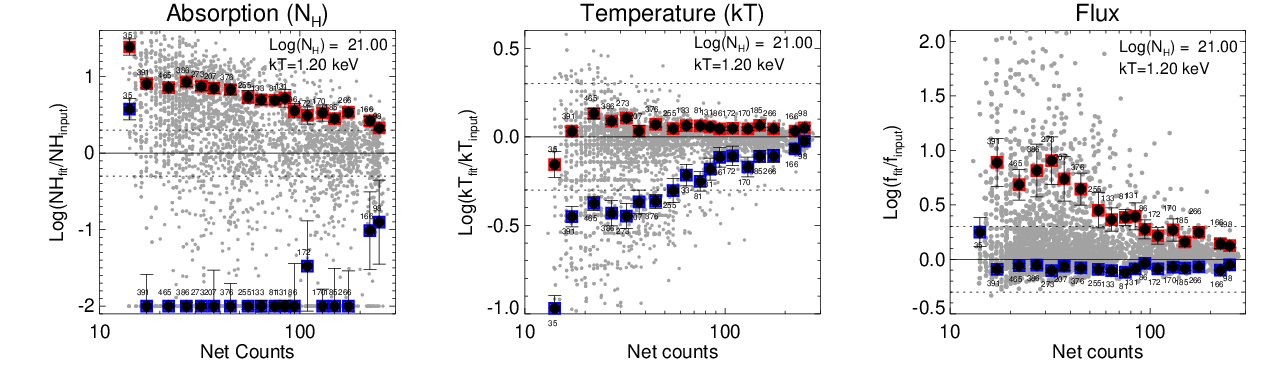
In Figure 2, we show, for two model spectra, the runs of best-fit Fx, NH, and kT as a function of the number of source counts. Also shown are the quantiles (Q and Q) computed for source net counts in the range 10–350. The upper and lower panels refer to a relatively hard and highly absorbed thermal source ( cm-2, keV), and to a softer, less absorbed source ( cm-2, keV), respectively, illustrating how model dependent our results are. We note in particular difficulties in constraining the absorption for the latter, less absorbed, model, for which lower limits to the parameter were often not restricted by the data for cases in which there were less than 100 net counts. In these cases, the blue squares representing the lower quantile limits are set to the lower limit of the allowed range we specified in the XSPEC fitting procedure—a factor of 100 less than the input value. This lack of sensitivity to low values occurs because of the limited soft X-ray response of ACIS-I; this has been eroded since launch by the gradual build-up of a molecular contamination layer that attenuates low-energy X-rays [9, e.g.]. This limitation places a constraint on the range of validity of our results in the sense that uncertainties in will be strictly accurate for cm2. For lower column densities both the and unabsorbed flux uncertainties are subject to systematic error, the latter being affected because it is dependent on the former. We return to this briefly in the verification of our method in Section V).
Another useful way to visualize our results is illustrated in Fig. 3 (upper and lower left panels). Here we show, for models with total counts in a given range (in this case 35–40 counts), the flux uncertainties/quantiles as function of input kT for different input values of (upper panel), and input for different input values of kT (lower panel). These figures illustrate that the dependence of uncertainties on model parameters is non-trivial and cannot easily be approximated analytically.
The three-dimensional thermal and non-thermal grids of simulations also allow us to aspects of the results easily in two dimensions (three dimensions is also of course possible, but challenging to interpret). Also illustrated in the central and right-hand panels of Fig. 3 is an example of how contour maps of the two-dimensional dependence of the positive and negative 1 relative flux uncertainties depends on and kT for the case of thermal spectra with 35–40 counts. To avoid discontinuous artefacts resulting from the limited sampling of our grid, these maps were produced by interpolating within the grids using a cubic spline function. We tested this method by interpolating in both NH for fixed kT values (top middle and right panels), and in kT for fixed NH values (bottom middle and right panels). The two approaches are in very good agreement, indicating that the log()–log(kT) space is well mapped, and that the approach is free from significant numerical instability or bias. The contour curves in Fig. 3 were computed for logarithmic relative error values equal to log([1.001, 1.1, 1.2, 1.3, 1.4, 1.5, 1.6, 1.7, 1.8, 1.9, 2.0, 2.5, 3.0, 4.0]).
At this point, we are able to give a full description of the Q-uncertainty for any value
of NH, kT or , and X-ray flux, for a given discrete range of net counts
(see Appendix) . However, as we mention in Section 2, the X-ray spectral simulations were
performed by adopting a negligible background fraction in the spectra.
Obviously, these results cannot be applied to those sources that suffer from higher background
contributions. For on-axis observations with Chandra ACIS-I, for which the PSF is very
compact, background can often be very low compared with source counts.
However, the PSF angular size increases with increasing off-axis
angle44
4
see http://cxc.harvard.edu/proposer/POG/html/chap4.html for details and
consequently the fraction of the photon events that comprise an extracted source spectrum
that can be attributed to background also increases. The background contribution can be
particularly significant for large off-axis angles (). We address this problem in the next section.
IV. How background photons affect the Q uncertainty


The results presented in Sections 2 and 3 corresponds to the case of sources with negligible background contamination, i.e., a background fraction less than 0.01. As noted above, this is generally not the case for Chandra, or many other X-ray observations, for which background events can be a significant or even dominant fraction of the extracted signal. High background contributions can potentially mask or bias the true nature of source X-ray spectra, make spectra noisy and compromise their interpretation and the ability to constrain spectral parameters in astrophysical modelling. In this section, we study this effect by means of further extensive MC simulations of background-affected spectra.
As before, the main goal is to estimate the dependence of the uncertainty of fitted spectral parameters on the intrinsic X-ray emission source model and the net photon counts of the spectra. We constructed a set of simulations based on eight different thermal and non-thermal X-ray emission models, simulated for different numbers of source and background counts. The background fraction of the simulations ranged between 0.001 to the limiting case of 1 (corresponding to a spectrum comprised of 100% background photons). We adopted RMF, ARF and background (BKG) files that correspond to a set of 100 X-ray sources randomly distributed over the field-of-view of the ACIS-I Chandra observation ID 4511 of the Cygnus OB2 association (see Albacete Colombo et al. 1 for further details of the observation).
Owing to the additional dimension of background fraction, we covered a more limited segment of the –kT plane than in the zero background grid employed in Sect. II. Thermal and non-thermal models were computed for a set of temperatures and/or index values that are listed in Table 1 and also illustrated in Figure 4. This amounted to a set of 14100 (thermal case) simulations for background fractions from 0.001 to 1, and for total events numbering 20, 30, 100 and 300 photons.
In the left of Figure 4, we show the the distribution of fit solutions for each model and for the different net counts in the spectra and background contamination fractions. At low absorption, the retrieved uncertainty is greater than that in temperature, while the opposite behavior occurs when becomes large, leading to a poor determination of temperature. This behavior arises simply because of the way the spectral “lever arm” acts: at low , there is little energy range over which the spectrum is significantly affected by absorption and purchase on is weak—as in the case of unconstrained lower limits noted in Section III above; conversely, there is a large energy range available to discern the spectral shape characteristics that are affected by temperature. At high , the opposite is true. Furthermore, uncertainty in temperature grows at higher temperatures because of the limited broad-band energy range available for our spectral fit. The spectrum tends to flatten out within the 8.0 keV bound we adopt; at higher energies where the temperature discrimination power largely lies for the hotter models, the ACIS-I effective area declines rapidly.
Closer inspection of the left panel in Figure 4 reveals some striation in the distributions of best-fit parameters, indicating that certain quantized values of temperature are slightly preferred over others. These artifacts result from the fits to spectra with low numbers of counts ( 30 photons) and the preferred temperatures are those of the plasma radiative loss model temperature grid. They occur when the uncertainties on the spectral fit are large, much larger than the grid quantization. This apparent fit bias only affects a very small fraction of the total and does not impose any bias on fit quantiles because the quantization effect is on a scale smaller than parameter estimation uncertainties.
A similar procedure to that for thermal models was followed to compute non-thermal models. A 3 grid of power-law indices () and absorbing column densities () was adopted, amounting to 9100 MC non-thermal simulations for background fractions in the range 0.001 to 1, and for 20, 30, 100 and 300 photons (see the right panel of Figure 4). The striation effect discernible for the thermal model fits does not occur for non-thermal models because the spectral model itself is analytic and not stored in quantized, tabulated form.
| Model | Thermal | Non-thermal | |||||
| # | NH | kT | Nsims | NH | Nsims | ||
| (cm-2) | (keV) | (cm-2) | |||||
| 1 | 1.01022 | 3.0 | 32017 | 1021 | 1.0 | 26031 | |
| 2 | 0.11022 | 1.2 | 35779 | 1021 | 3.0 | 29467 | |
| 3 | 0.11022 | 3.0 | 31413 | 1021 | 5.0 | 29304 | |
| 4 | 0.331022 | 3.0 | 49918 | 1022 | 1.0 | 21967 | |
| 5 | 3.31022 | 1.2 | 50159 | 1022 | 3.0 | 15269 | |
| 6 | 1.01022 | 1.2 | 48968 | 1022 | 5.0 | 23032 | |
| 7 | 33.01022 | 3.0 | 46859 | 1023 | 1.0 | 22730 | |
| 8 | 10.01022 | 3.0 | 31762 | 1023 | 3.0 | 18776 | |
| 9 | 0.11022 | 5.0 | 45730 | 1023 | 5.0 | 7172 | |
| 10 | 0.331022 | 5.0 | 44960 | ||||
| 11 | 1.01022 | 5.0 | 41042 | ||||
| 12 | 3.31022 | 5.0 | 34020 | ||||
| 13 | 10.01022 | 5.0 | 45116 | ||||
| 14 | 33.01022 | 5.0 | 49918 | ||||
In order to get a quantitative estimate of the uncertainty in best-fit spectral parameters, we compute their relative errors and respective quantiles as a function of the background fraction. Uncertainties correlate linearly with the background fraction of the simulated spectra, being well described by a function of the form
| (1) |
The coefficients of such a relationship are not the same for all spectral models even if they have the same net numbers of counts in the simulated spectra. They depend on the emission characteristics of the source, as well as the signal-to-noise ratio of the simulations. We evaluated the linear dependence of all the fourteen thermal, and nine non-thermal, models and computed the explicit dependence of Q on bkg_frac. In Table 1, we list the parameters of the background affected spectral models to map -kT or - planes, and the total of simulations performed for each one. Of the coefficients A (the slope) and B (the intercept), the latter agrees with the 1 quantile error estimation for MC simulations of spectra in which the background fraction is negligible or zero (bkg_frac 0.01). We thus can rewrite Equation 1 as
| (2) |
In Table 7 of the Appendix we list explicit coefficients computed from the uncertainty curves for 20, 30, 100 and 300 photons in background-affected MC simulated spectra. Such coefficients represent the change of the uncertainty estimation Q0 due to the influence of background photons in the net counts of the X-ray spectra. The most straightforward way to get the adequate coefficient for a given X-ray source is by choosing the most representative model for the true source X-ray spectrum.
We can linearly interpolate within the grid of results to obtain bi-dimensional planes of the
uncertainties in any given parameter as a function of background fraction for a given number
of total counts between 20 and 300. As an example, in Figure 5 we show how
the uncertainty in X-ray flux increases with the background fraction, and how it is more tightly
constrained as the net counts in the spectra increases. The thermal ”model 1” ( and kT=3.0 keV; see the Figure 5) was chosen as the example for
this figure, and corresponds to the most representative model of the sources in the Cyg OB2
Association (which are mostly T Tauri stars; Albacete Colombo et al. 1, Flaccomio et al., 2016, this issue;
Drake et al., 2016, this issue). We discuss the Cyg OB2 case in more detail in Section V below.

V. Testing uncertainties of X-ray model parameters for faint Cyg OB2 sources

One main motivation of this work is to estimate the uncertainties on luminosities and spectral parameters expected for sources yet to be observed, based on the anticipated ACIS-I Chandra X-ray spectrum. However, another use is to cross-check, or even calculate, the uncertainty obtained from the fitting process and to give rough estimates in those cases in which the calculation of uncertainties fails formally (e.g. when the error command in XSPEC fails due to numerical issues). As a first application and verification of our method, we use real data and spectra that have been extracted as part of the Cygnus OB2 Chandra Legacy Survey (Drake et al. this issue). In this context, our aim is: i) to give spectral fit constraints from our quantile method for Cyg OB2 sources; ii) to compare the uncertainties in the X-ray spectral parameters for faint sources with those results obtained from non-interactive spectral fits presented in Flaccomio et al. (this issue).
Following results of the analysis presented by [11], a large fraction of the Cyg OB2 sources have been detected at large off-axis angles with ACIS-I. As we have noted above, the PSF degradation of the ACIS-I detector with increasing off-axis angle means the relative contribution of background photons to source events can be relatively large, which can affect the way in which spectral fitting converges as well as the uncertainty in the computed spectral solution. In fact, of the 7924 Cyg OB2 sources, just 10 have background fractions less than . The median of the distribution of background fractions is 0.36, with some background fractions being as high as 0.9. Thus, if we want to get an unbiased Quantile error estimation, it is strictly necessary to include the background dependency while accounting for the different X-ray emission characteristics of the sources. We employ a set of nine different optically-thin thermal plasma models that in the kT- plane represent the range in the uncertainty of parameters and flux as a function of the different background fractions (see Fig 6). This procedure allows us to get a much more precise estimate of the influence of the background on parameter uncertainties than we would be able to from the use of a single average model.
The complete catalog of Cyg OB2 sources in the survey comprises a total of 7924 X-ray objects
[11]. Of these, 4975 have less than 20 net photons, i.e. about 62% of
the whole source sample. Flaccomio et al (this issue, 2016) have performed spectral fitting of X-ray spectra
for sources with more than 20 and less than 350 counts, and if we restrict the sample to this
range we get a total of 2755 sources for which X-ray spectral fits could give an
error estimation for the model parameters and flux. We further limit ourselves to X-ray sources
that were classified as members of the Association (Kashyap et al, 2016, this issue) and whose X-ray
spectral fitted parameters are in the range of [–] and
kT = [0.5-8] keV. This subsample contains 1718 sources, and corresponds to 20% of the entire sample
Cyg OB2 members.
V.1. Comparing errors from spectral fits with Quantile estimates
In this subsection we study the goodness of our method in the determination of uncertainties of the X-ray parameters computed from spectral fits. To do that we need to accounts for two approaches: i) to compute the fit error of a given parameter (fit_err) via the XSPEC error command, which consist in the 1 error computed from the covariance matrix in the spectral fits of Cyg OB2 stars (see Flaccomio et al. this issue); ii) to determinate the respective Q-uncertainties computed from our 2D Quantile maps corrected by the influence of the individual X-ray background fraction of the Cyg OB2 sources. The ratio between these two quantities is show as grey crosses in the Figure 7 (upper panel).
In order to give a robust quantitative estimates of the reliability of our method, we made use of a statistical estimator known as the Forward Moving Averages (FMA), which can be computed from the cumulative unweighted averages of a given set of sorted sample data points. We sort all the fit_err/Q values in ascending order of background fraction. The FMA starts from the first fit_err/Q value until the next recomputed current () value, to the last adopted data point of our sample. Further details can be found from the help of the ts_smooth55 5 http://www.exelisvis.com/docs/TS_SMOOTH.html. IDL task. We use this technique on parameters , kT, and unabsorbed X-ray flux, to compute the goodness quantile error prediction with respect to the errors computed from X-ray spectral fits. As is shown in Figure 7, the majority of distributed FMA values are less than 10–12 %, even for higher background fractions.
While the combined positive and negative uncertainties from our approach are in excellent agreement with uncertainties from spectral fits to observed data, we note that the one-sided uncertainties do show some systematic deviations, albeit at levels of only % or so. This is revealed by the spread in the colored dots in the top panels of Figure 7, and in the separation of the distributions in the lower panel. There are good reasons why the uncertainties should not be in perfect agreement. Fits to observed data use only an approximation to the true instrument response—represented by the ARF and RMF files noted in Section II—and also assume a spectral model that will diverge from the real emission spectrum of a plasma at some level. In contrast, the simulations are fit with exactly the same models used to generated them, such that the difference between the retrieved and input spectral parameters results from Poisson noise. In the regime of a large number of photon counts and relatively low background, these systematic differences will be more important.
Systematic errors in fitted spectral parameters due to ”imperfect” instrument response functions and plasma model spectra will lead to systematic errors in the derived quantile because the point of interpolation in the 2D quantile maps will be offset from where it should ideally be. In regions of these maps that are relatively flat, this interpolation error will be small. However, there are some regions of these quantile planes that have larger gradients, and in these regions the systematic error in the derived quantile can be larger.
At the low signal-to-noise end, we have also encountered in Section III the low hydrogen
column density cases in which the spectral fit simulations are occasionally unable to constrain the lower
bound fit errors. Indeed, the discrepancy in the two-sided errors is largest for the unabsorbed
flux, which in the bandpass of interest here is highly dependent on the uncertainty in . The
two-sided errors are somewhat more discrepant for unabsorbed flux than for the absorption or
kT plasma temperature, which are in excellent agreement. Chandra ACIS-I spectra have good observational
leverage on plasma temperature for typical Cyg OB2 sources. However, modeling degeneracies
between and kT are less well constrained for less absorbed stars with low signal-to-noise
spectra, potentially leading to inaccuracy in the error estimate for the unabsorbed flux.
In the light of this discussion, we conclude that in general the error estimation from spectral fitting
is in very good agreement with our quantile estimates. Our method then represents a reliable means for
error estimation in X-ray spectral parameters whenever the model fit to the X-ray data cannot provide it,
as well as for observation planning in which data are not yet in-hand. The method can also be applied to
promptly estimate the errors in spectral parameters for previously studied X-ray source populations when
uncertainties where not published or are otherwise unavailable.
VI. Summary
We present a new method for the estimation of errors in X-ray spectral parameters and fluxes of faint sources detected by ACIS-I onboard Chandra. X-ray sources in the range of 10 to 350 net photons are generally not well-suited to quantitative spectral analysis. Simple X-ray spectral modeling of such weak sources can suffer from ill-constrained solutions and mismatches between true and modeled parameters, combined with unrealistic estimation of the true uncertainties.
Here, we have described an original treatment that resolves these problem by means of an extensive set of MC simulations of faint X-ray spectra. As representative cases, we adopted absorbed optically-thin thermal plasma models and power-law continua that are commonly employed to interpret a wide range of astrophysical sources of X-rays. We fitted simulated spectra for a wide range of absorption, plasma temperature and power-law index. We studied the relative error distributions of retrieved parameters and fluxes and describe fits in terms of 1 quantiles. We computed parametric curves of quantiles as a function of given input model parameters and interpolated within these to compute bi-dimensional maps. Such a set of maps provides an estimation of the true error in spectral parameters whenever it is not possible to determine these adequately from a direct spectral fit.
Our method makes it possible to improve statistical studies of objects in which a large fraction have a low number of counts. As an example, we have applied this method to sources in the Chandra Cygnus OB2 Legacy Survey and the properties of faint X-rays sources that mostly correspond to young low-mass stars. The uncertainties estimated using the quantile method presented here and from spectral fitting applied to the observations are in excellent agreement, and generally at a level of 10 % or better.
Finally, our method and data enable the computation of the exposure times required for surveys and individual pointed observations to reach a given uncertainty in derived spectral parameters. The results of this work will be made publicly available in an on-line tool in the near future.
References
- [1] Albacete Colombo, J. F., Flaccomio, E., Micela, G., Sciortino, S., & Damiani, F. 2007, A&A, 464, 211
- [2] Anders, E. & Grevesse, N. 1989, Geochim. Cosmochim. Acta, 53, 197
- [3] Arnaud, K. A. 1996, in Astronomical Society of the Pacific Conference Series, Vol. 101, Astronomical Data Analysis Software and Systems V, ed. G. H. Jacoby & J. Barnes, 17
- [4] Broos, P. S., Townsley, L. K., Feigelson, E. D., et al. 2010, ApJ, 714, 1582
- [5] Cash, W. 1979, ApJ, 228, 939
- [6] Guarcello, M. G., Drake, J. J., Wright, N. J., et al. 2015, ArXiv e-prints
- [7] Hong, J., Schlegel, E. M., & Grindlay, J. E. 2004, ApJ, 614, 508
- [8] Maggio, A., Sciortino, S., Collura, A., & Harnden, Jr., F. R. 1995, A&AS, 110, 573
- [9] O’Dell, S. L., Swartz, D. A., Tice, N. W., et al. 2013, in Society of Photo-Optical Instrumentation Engineers (SPIE) Conference Series, Vol. 8859, Society of Photo-Optical Instrumentation Engineers (SPIE) Conference Series, 0
- [10] Smith, R. K., Brickhouse, N. S., Liedahl, D. A., & Raymond, J. C. 2001, ApJ, 556, L91
- [11] Wright, N. J., Drake, J. J., Guarcello, M. G., et al. 2014, ArXiv e-prints
- [12] Wright, N. J., Drake, J. J., Guarcello, M. G., Kashyap, V. L., & Zezas, A. 2015, ArXiv e-prints
Here we present bi-dimensional maps of the Q uncertainty for flux and spectral parameters of thermal and non-thermal models. As examples, we show 2D quantile maps restricted to 90 to 100 X-ray photons in the simulated spectra. See the captions for a description of individual panels. For each case, movies covering all ranges of parameters investigated as a function of the X-ray net counts in the spectra are presented as on line material.


| Model | 20 ph | 30 ph | 100 ph | 300 ph |
|---|---|---|---|---|
| 1 | 0.56999999 , -0.79058786 | 0.29294601 , -0.35787199 | 0.18000001 , -0.32236677 | 0.11482079 , -0.087020800 |
| 2 | 1.5800000 , -1.5800000 | 0.43000001 , -0.43000001 | 0.18000001 , -0.18000001 | 0.029938766 , -0.029938766 |
| 3 | 1.0000000 , -1.0000000 | 0.59519789 , -0.59519789 | 0.11634470 , -0.11634470 | 0.10000000 , -0.10000000 |
| 4 | 0.049715455 , -1.0000000 | 0.62929869 , -3.2919384 | 0.12753756 , -0.41111881 | 0.00016174661 , -0.17443736 |
| 5 | 0.11171015 , -0.61089794 | 0.079572385 , -0.52813251 | 0.079557867 , -0.11617288 | 0.043629286 , -0.044922529 |
| 6 | 1.3000000 , -2.0934750 | 0.67000002 , -0.75529767 | 0.093786779 , -0.25956268 | 0.086018041 , -0.057652803 |
| 7 | 0.88999999 , -0.57335823 | 0.27781488 , -0.44000000 | 0.18754265 , -0.062686584 | 0.16403699 , -0.039999999 |
| 8 | 0.58999997 , -0.60203861 | 0.41679498 , -0.35140125 | 0.42944980 , -0.12969924 | 0.28124141 , -0.022691981 |
| 9 | 0.87000000 , -0.87000000 | 0.49000001 , -0.49000001 | 0.23999999 , -0.23999999 | 0.11832534 , -0.11832534 |
| 10 | 0.38999999 , -0.790000 | 0.27743047 , -0.440000 | 0.063187085 , -0.28924141 | 0.034755657 , -0.029999999 |
| 11 | 0.63999999 , -0.64599982 | 0.10191273 , -0.61887488 | 0.11436878 , -0.18611558 | 0.030987269 , -0.11433628 |
| 12 | 0.38999999 , -0.69138395 | 0.28999999 , -0.37843546 | 0.21054822 , -0.20999999 | 0.067875243 , -0.19371328 |
| 13 | 0.58999997 , -0.69999999 | 0.50999999 , -0.57290317 | 0.44196881 , -0.10809053 | 0.23690649 , -0.088281814 |
| 14 | 1.0000000 , -1.0000000 | 0.23863081 , -0.23000000 | 0.16731354 , -0.096115480 | 0.029999999 , -0.087420713 |
| Model | 20 ph | 30 ph | 100 ph | 300 ph |
|---|---|---|---|---|
| 1 | 1.1791490 , -0.69999999 | 1.0236216 , -0.38275211 | 0.35172140 , -0.16000000 | 0.070000000 , -0.12034473 |
| 2 | 0.59865859 , -0.40000001 | 0.15000001 , -0.22137435 | 0.079999998 , -0.10181730 | -0.0058132137 , -0.020912962 |
| 3 | 1.6737583 , -1.0000000 | 0.40438804 , -0.67145439 | 0.25332680 , -0.12570339 | 0.080397019 , -0.032017613 |
| 4 | 1.5045421 , -0.19886096 | 1.0100729 , -0.70493358 | 0.35332554 , -0.19089511 | 0.12219090 , -0.064251043 |
| 5 | 1.0285405 , -0.22003141 | 1.3540962 , -0.14531649 | 0.16706693 , -0.073932650 | 0.048124737 , -0.019780164 |
| 6 | 1.7827508 , -1.7827508 | 0.77129511 , -0.77129511 | 0.13526567 , -0.13457852 | 0.020276173 , -0.14306573 |
| 7 | 1.9000000 , -1.9000000 | 1.6500000 , -1.6500000 | 1.3150349 , -0.89999998 | 0.68300091 , -0.15976273 |
| 8 | 1.6700000 , -0.56000000 | 1.5449302 , -0.46316759 | 0.43428638 , -0.35728049 | 0.12876973 , -0.17824362 |
| 9 | 1.1222106 , -0.33227760 | 1.1170738 , -0.14316164 | 0.38273876 , -0.072976206 | 0.058509901 , -0.092050602 |
| 10 | 0.98000002 , -0.44000000 | 0.68061929 , -0.27748997 | 0.54441994 , -0.16165912 | 0.21343224 , -0.15936723 |
| 11 | 0.68000001 , -0.68000001 | 0.55418089 , -0.19408860 | 0.69571872 , -0.22827677 | 0.13584275 , -0.12354602 |
| 12 | 1.7900000 , -0.28999999 | 1.3700000 , -0.25924568 | 1.2029648 , -0.14825462 | 0.36546867 , -0.050000001 |
| 13 | 1.90000 , -0.70999998 | 1.70000 , -0.52999997 | 1.5044654 , -0.41568087 | 0.48996156 , -0.33525367 |
| 14 | 1.14000 , -0.63999999 | 0.990000 , -0.34000000 | 0.80259332 , -0.19586915 | 1.2665589 , -0.15802399 |
| Model | 20 ph | 30 ph | 100 ph | 300 ph |
|---|---|---|---|---|
| 1 | 0.600000 , -0.330000 | 0.54025202 , -0.11000000 | 0.10682827 , -0.050495573 | 0.040233470 , -0.036603905 |
| 2 | 0.60000002 , -0.22000000 | 0.26444894 , -0.075128038 | 0.14690279 , -0.035009770 | 0.0088736486 , -0.0088736486 |
| 3 | 0.61000001 , -0.330000 | 0.46442869 , -0.022708227 | 0.091840132 , -0.074119511 | 0.033806779 , -0.041856700 |
| 4 | 0.32547463 , 0.22537710 | 0.71408237 , -0.0064318752 | 0.094341279 , -0.068698972 | -0.0054402611 , -0.019880270 |
| 5 | 0.63611881 , -0.58999997 | 0.38808347 , -0.36155323 | 0.21717026 , -0.21975059 | 0.16171609 , -0.074638882 |
| 6 | 0.69999999 , -0.69999999 | 0.55000001 , -0.55000001 | 0.23215765 , -0.097066930 | 0.15446032 , -0.041110827 |
| 7 | 1.8000000 , -1.8000000 | 1.3300000 , -1.3300000 | 0.62809720 , -0.20183422 | 0.38454859 , -0.19000000 |
| 8 | 1.8800000 , -0.49000001 | 1.6358418 , -0.24090247 | 0.83024481 , -0.15000001 | 0.28627373 , -0.12124413 |
| 9 | 0.33069971 , -0.33069971 | 0.22148313 , -0.22148313 | 0.077915734 , -0.062867283 | 0.024395005 , -0.040764767 |
| 10 | 0.38207975 , -0.38999999 | 0.28651545 , -0.070000000 | 0.072748663 , -0.029204307 | 0.020000000 , -0.063466439 |
| 11 | 0.27969115 , -0.27969115 | 0.20694499 , -0.060739656 | 0.086205055 , -0.049771037 | 0.00058630777 , -0.068272805 |
| 12 | 0.38270376 , -0.38999999 | 0.29421943 , -0.27000001 | 0.12630442 , -0.19000000 | 0.029999999 , -0.13910898 |
| 13 | 0.900000 , -0.41000000 | 0.770000 , -0.28565844 | 0.63059201 , -0.060723811 | 0.23391268 , -0.070676279 |
| 14 | 1.3000000 , -1.3000000 | 0.60592199 , -0.80000001 | 0.51963257 , -0.23999999 | 0.039999999 , -0.15035874 |
| Model | 30 ph | 100 ph | 300 ph |
|---|---|---|---|
| 1 | 0.25650181 , -1 | 0.12430397 , -0.50202637 | 0.18169266 , -1.1245344 |
| 2 | 0.40523864 , -0.30208423 | 0.11622960 , -1.1318363 | 0.28298807 , -2.9794969 |
| 3 | 0.22044614 , -1 | 0.55048480 , -0.051447758 | 0.52473601 , -3.2887644 |
| 4 | 0.500000 , -4.6345525 | 0.16597746 , -0.97468140 | 0.066336864 , -0.31664817 |
| 5 | 0.12215644 , -0.79181550 | 0.10350067 , -0.29293987 | 0.074220414 , -0.16425698 |
| 6 | 0.089567717 , -1.0198450 | 0.23257742 , -0.25237991 | 0.096013813 , -0.17154169 |
| 7 | 0.570000 , -0.250000 | 0.57413525 , -0.34905480 | 0.37936515 , -0.28201250 |
| 8 | 0.27773648 , -1.2329168 | 0.36234157 , -0.15427702 | 0.19328749 , -0.14761850 |
| Model | 30 ph | 100 ph | 300 ph |
|---|---|---|---|
| 1 | 0.19699650 , -0.081710183 | 0.052672355 , -0.093241764 | 0.039347859 , -0.050306389 |
| 2 | 0.25117132 , -0.10266247 | 0.078957645 , -0.067741463 | 0.038052451 , -0.060455948 |
| 3 | 0.21329448 , -0.016207271 | 0.22695826 , -0.010517673 | 0.16103488 , -0.046310364 |
| 4 | 0.400000 , -0.500000 | 0.097128085 , -0.33579614 | 0.0047083283 , -0.23929186 |
| 5 | 0.082105410 , -0.29366887 | 0.091130471 , -0.13137739 | 0.040882831 , -0.059770894 |
| 6 | 0.12310893 , -0.28904541 | 0.22853133 , -0.14899948 | 0.10236678 , -0.12266170 |
| 7 | 1.50000 , -0.600000 | 0.800000 , -0.500000 | 0.35792970 , -0.52635195 |
| 8 | 0.43658025 , -0.49066309 | 0.16724924 , -0.19066881 | 0.067044326 , -0.043196329 |
| Model | 30 ph | 100 ph | 300 ph |
|---|---|---|---|
| 1 | 0.17029916 , -0.027228378 | 0.053110142 , -0.043069600 | 0.027653891 , -0.025060421 |
| 2 | 1.0406915 , 0.012650287 | 0.077507279 , -0.039221376 | 0.073060202 , -0.035090637 |
| 3 | 0.77695532 , 0.013296297 | 0.90757450 , -0.062870060 | 0.53249562 , -0.12403132 |
| 4 | 0.23904451 , -0.040587606 | 0.048288826 , -0.046017530 | 0.0500000 , -0.041524861 |
| 5 | 0.58708610 , -0.093046929 | 0.31389033 , -0.23559708 | 0.12070400 , -0.12857378 |
| 6 | 0.540000 , -0.55078238 | 1.3023024 , -0.51431365 | 0.41070973 , -0.56508111 |
| 7 | 1.1208722 , -0.10905732 | 1.1694971 , -0.072869982 | 0.38194822 , -0.13259251 |
| 8 | 2.2073709 , -0.56064182 | 1.1706366 , -0.44397279 | 0.40848299 , -0.30326180 |